Decoherence and classicalization of continuous-time quantum walks on graphs

Abstract

We address decoherence and classicalization of continuous-time quantum walks (CTQWs) on graphs. In particular, we investigate three different models of decoherence, and employ the quantum-classical (QC) dynamical distance as a figure of merit to assess whether, and to which extent, decoherence classicalizes the CTQW, i.e. turns it into the analogue classical process. We show that the dynamics arising from intrinsic decoherence, i.e. dephasing in the energy basis, do not fully classicalize the walker and partially preserves quantum features. On the other hand, dephasing in the position basis, as described by the Haken-Strobl master equation or by the quantum stochastic walk (QSW) model, asymptotically destroys the quantumness of the walker, making it equivalent to a classical random walk. We also investigate the speed of the classicalization process, and observe a faster convergence of the QC-distance to its asymptotic value for intrinsic decoherence and the QSW models, whereas in the Haken-Strobl scenario, larger values of the decoherence rate induce localization of the walker.

1 Introduction

Quantum walks (QWs) are the quantum-mechanical counterpart of classical random walks (RWs) kempe003 ; venegas2012 ; xia20 ; kadian21 ; frigerio21 . If the walker evolves in discrete temporal steps, we talk about discrete-time QWs, while in continuous-time quantum walks (CTQWs) time is a real parameter aharonov93 ; farhi98 . In this work, we focus on continuous-time quantum walks. Quantum walks on graphs are used to describe the transport of energy or information across a given structure in several physical, chemical and biological systems mulken2011 ; mulken07 ; razzoli11 ; maciel20 . They also proved to be powerful tools for building quantum algorithms ambainis2003 ; portugal18 and provide a universal model of quantum computation childs09 ; Wang20 ; Herrman2022 .

Experimental implementations of quantum walks unavoidably involve the interaction with an external environment, and a question arises on whether, and to which extent, the open quantum system dynamics of a quantum walker is detrimental to its quantum features. In turn, the thorough characterisation of decoherence effects in CTQWs is a key ingredient for their use in quantum technology and, in particular, to envisage strategies that may mitigate or cancel out noise. Several studies investigated how noise stemming from the interaction between the system and the environment affects the dynamics of quantum walks norio05 ; plenio08 ; caruso09 ; schreiber11 ; benedetti16 ; tama17 ; benedetti19 ; Kurt20 . Different effects may emerge, such as localization, transition toward a classically distributed walker schreiber11 ; benedetti16 ; benedetti19 , but also an improvement in excitation transport efficiency plenio08 ; caruso09 ; tama17 ; Kurt20 . However, if a QW loses all of its quantum features and becomes a classical RW, then any potential quantum advantage related to the quantum process is lost as well.

In this paper, we study if decoherence can turn a continuous-time quantum walk over a graph into the corresponding classical random walk. We refer to this phenomenon as classicalization. In order to make our analysis quantitative, we use a fidelity-based measure of non-classicality, referred to as quantum-classical distance, that quantifies the differences between the dynamics of a quantum and a classical walker on a given graph gualtieri20 . Recently, this quantity has been also used as a tool to design optimal quantum walks frigerio22 . We use this distance to assess if and to which extent decoherence makes the quantum evolution more similar to its classical counterpart, at least asymptotically, with respect to the ideal noiseless case.

In the following, we study three different models of decoherence. First, we investigate intrinsic decoherence Milburn91 , i.e. decoherence in the Hamiltonian basis, then we shift our focus to two different mechanisms of decoherence in the position basis. In particular, we consider dephasing induced by the Haken-Strobl master equation haken73 and then we analyse the interplay of unitary and irreversible dynamics using the quantum stochastic walk framework QuantumStochasticWalk . We show that intrinsic decoherence is not able to completely classicalize the walker: residual quantumness is preserved, and the quantum walker dynamics departs from the corresponding classical one. We give the analytic expressions for the asymptotic value of the quantum-classical distance over the complete, cycle and star graphs. On the other hand, the two models of decoherence in the position basis completely suppress the quantum features of the coherent process, nullifying the quantum-classical distance.

As we will see in detail, some general properties of the quantum-classical distance do not depend on the decoherence model: it reaches an asymptotic value which does not depend on the decoherence rate and its qualitative behavior is not dependent on the size of the graph, nor the considered topology. On the other hand, we show that speed of the convergence of the quantum-classical distance to its asymptotic value is influenced by the noise parameter with a non-universal behavior. For intrinsic decoherence and for the quantum stochastic walk model, we observe that a larger value of the decoherence parameter leads to a faster convergence, whereas for the Haken-Strobl master equation we see an inversion, such that after a threshold value of the noise rate the quantum-classical distance decays slower.

The paper is organized as follows. In Section 2, we establish notation and briefly review classical and quantum walks, the master equation approach for noisy quantum walks, and the quantum-classical distance. In Section 3. we investigate the effects of intrinsic decoherence on CTWQs, while Section 4 is devoted to the study of decoherence in the position basis. In Section 5 we draw conclusions, and provide some concluding remarks.

2 Preliminary concepts

Let us consider a finite, simple, undirected, connected graph $G(V,E)$, where $V$ is the set of vertices, also called nodes, and $E$ the set of edges. The cardinality of $V$ sets the dimension of the graph, i.e. the number of nodes $N=|V|$. A graph is uniquely identified by its Laplacian matrix $L=D-A$, where $A$ is the adjacency matrix and $D$ is a diagonal degree matrix nica2018 . In particular, $A_{jk}=1$ if vertices $j$ and $k$ are connected (with $j\neq k$), and zero otherwise, and $D_{jj}=d_{j}$ is the vertex degree of the node, i.e. the number of edges connecting the $j$-th node to the others. $L$ is a positive semi-definite matrix and completely determines the classical evolution of a walker on a graph. The dynamics of a classical walker initially localized on node $j$ may be described by the diagonal density matrix

$$\mathcal{E}_{C}[\rho_{j}](t)=\sum_{k=1}^{N}p_{kj}(t)|k\rangle\!\langle k|.$$ (1)

where $p_{kj}(t)=\langle k|e^{-\nu Lt}|j\rangle$ is the classical transition probability from node $j$ to node $k$, $\nu$ is the transition rate, $\{|k\rangle\}_{k=1}^{N}$ is the complete orthonormal basis which describes localized states of the walker on the $N$ nodes of the graph and $\rho_{j}=|j\rangle\!\langle j|$ is the initial state. The map $\mathcal{E}_{C}$ describes a continuous-time random walk (CTRW) on the graph $G$. On the other hand, the purely coherent quantum evolution of a CTQW is obtained by promoting the Laplacian to the system’s Hamiltonian $H=\nu L$ farhi98 (though this is not the only possible choice for a CTQW generator frigerio21 ; wong2016 ). Without loss of generality we can set the transition rate to $\nu=1$ and $\hbar=1$. The unitary evolution of the quantum walk is thus given by $\ket{\psi(t)}=e^{-iHt}\ket{j}$, where $\ket{j}$ denotes the initial localized state.

2.1 Noisy quantum walks

If the walker interacts with an external environment, its evolution is no longer unitary and can be described, within the Markovian approximation, by a master equation in the Lindblad form, i.e.

$$\frac{d\rho(t)}{dt} =-i\left[L,\rho(t)\right]+\sum_{k}\gamma_{k}\mathcal{D}\left[O_{k}\right]\rho(t)\,.$$ (2)

Here $\mathcal{D}$ is the Limbladian superoperator, defined as $\mathcal{D}\left[A\right]\rho=A\rho A^{\dagger}-\frac{1}{2}\{A^{\dagger}A,\rho\}$ with the brackets $\{A,B\}=AB+BA$ denoting the usual anticommutator, $O_{k}$ are the Lindblad operators and $\gamma_{k}\geq 0$. The main goal of this work is to investigate if, and to which extent, the presence of environmental noise makes the quantum evolution of a walker on a graph more similar to its classical counterpart (that is described by Eq. (1)), compared to the ideal noiseless scenario. In particular, we consider three models of noisy quantum walks whose dynamics is induced by three master equations that describe dephasing in some basis of choice.

At first, we focus on decoherence in the energy basis, corresponding to the following master equation

$$\frac{d\rho(t)}{dt} =-i\left[L,\rho(t)\right]-\frac{\gamma}{2}[L,[L,\rho(t)]]\,,$$ (3)

which describes intrinsic decoherence of a quantum system. It has been derived Milburn91 by assuming that at short timescales a quantum system evolves as a stochastic sequence of random unitary operators. The parameter $\gamma\geq 0$ is referred to as the decoherence rate, and $L$ is the graph Laplacian. From an operational point of view, intrinsic decoherence corresponds to a randomized quadratic perturbation l2pert .

We then consider two different models of decoherence in the site (position) basis. The first one corresponds to the Haken-Strobl master equation haken73 , which reads

$$\frac{d\rho(t)}{dt}= -i\left[L,\rho(t)\right]+\gamma\,\sum_{k}\mathcal{D}[P_{k}]\rho(t)\,,$$ (4)

where $\gamma\geq 0$ is the decoherence rate and $P_{k}=\outerproduct{k}{k}$ are the site-projector operators. It can be shown haken73 that the Haken-Strobl master equation corresponds to a system with a tight-binding Hamiltonian affected by stochastic noise describing thermal Gaussian fluctuations of the on-site energies. The decoherence parameter $\gamma$ is related to the variance of the thermal fluctuations. The Haken-Strobl master equation finds applications in the description of a single excitation transport, e.g. in an $N$-site chain subject to dephasing induced by the interaction with a fluctuating environment Rebentrost09 .

A second model of decoherence in the site basis is provided by the quantum stochastic walk (QSW) approach QuantumStochasticWalk . The QSW formalism axiomatically generalizes a classical random process to a quantum stochastic process, where the topology of the underlying graph imposes constraints on the dynamical evolution of the walker. It is described by the following master equation Caruso

$$\frac{d\rho(t)}{dt}=-(1-p)\,i\,[L,\rho(t)]+p\sum_{kj}\mathcal{D}[P_{kj}]\rho(t)\,.$$ (5)

Here $p\in[0,1]$ quantifies the interplay between unitary ($p=0$) and irreversible ($p=1$) dynamics and the $P_{kj}=L_{kj}\outerproduct{k}{j}$ are the jump operators, with $L_{kj}=\bra{k}L\ket{j}$. This model generalizes both the QW and the RW on the graph by continuously interpolating between the two dynamics with a single real mixing parameter $p$. This model has been employed to investigate the role of environmental noise in assisting the transport of energy or information across a network, such as a light-harvesting complex in a photosynthetic process Caruso ; caruso09 ; tama17 ; Kurt20 .

2.2 The quantum-classical distance

In order to compare the dynamics of different quantum walks models, and to quantify the differences between quantum and classical evolutions, we use a recently introduced dynamical distance based on fidelity gualtieri20 . Given two dynamical maps, describing a classical $\mathcal{E}_{C}[\rho_{cl}]$ and a quantum $\mathcal{E}_{Q}[\rho_{cl}]$ evolution, the QC-distance $D_{\text{\tiny QC}}(t)$ between them is defined as gualtieri20 :

$$D_{\text{\tiny QC}}(t)\doteq 1-\underset{\rho_{cl}}{\text{min}}\,\mathcal{F}\left(\mathcal{E}_{C}[\rho_{cl}](t),\mathcal{E}_{Q}[\rho_{cl}](t)\right)\,,$$ (6)

where $\rho_{cl}$ is an initial classical state of the walker, i.e. a statistical operator diagonal in the node basis, and $\mathcal{F}(\mathcal{E}_{C}[\rho_{cl}],\mathcal{E}_{Q}[\rho_{cl}])$ is the quantum fidelity between the classically and quantum evolved states, i.e. $\mathcal{F}(\rho,\sigma)=\left[\Tr\sqrt{\sqrt{\rho}\sigma\sqrt{\rho}}\right]^{2}$. The minimization in Eq. (6) is achieved, for every graph, by a localized state $\rho_{j}$ gualtieri20 , hence we shall focus on such initial states only. An interesting feature of this measure of non-classicality is that, for noiseless unitary quantum dynamics, it has an horizontal asymptote which depends only on the total number of nodes $N$, i.e. $\lim_{t\rightarrow\infty}D_{\text{\tiny QC}}(t)=1-\frac{1}{N}$. In the next Section, we use the QC-distance as a figure of merit to assess the robustness of CTQW against decoherence. In particular, we compute the QC-distance between the classically evolved state $\mathcal{E}_{C}[\rho_{j}](t)$ defined in Eq. (1), and the quantum state described by a CPTP-map modeling decoherence in some basis of choice.

3 Decoherence in the energy basis

Let us consider a quantum walker subject to the intrinsic decoherence process described by the master equation (3). The solution for an initial localized state $\rho_{j}=\outerproduct{j}{j}$, is given by

$$\mathcal{E}_{L} [\rho_{j}](t)=\sum_{n,p}\langle\lambda_{n}|\rho_{j}|\lambda_{p}\rangle e^{-i(\lambda_{n}-\lambda_{p})t-\frac{1}{2}\gamma(\lambda_{n}-\lambda_{p})^{2}t}|\lambda_{n}\rangle\!\langle\lambda_{p}|\,,$$ (7)

where $\{\lambda_{n}\}_{n=1}^{N}$ and $\{|\lambda_{n}\rangle\}_{n=1}^{N}$ are respectively the eigenvalues and eigenvectors of $L$, i.e. $L|\lambda_{n}\rangle=\lambda_{n}|\lambda_{n}\rangle$. Eq. (7) represents decoherence in the energy basis, and may also be expressed in the following form:

$$\mathcal{E}_{L}[\rho_{j}](t)=\int dy\,g(y|\,0,\sigma)\,\,e^{-iL(t+y)}\rho_{j}e^{iL(t+y)}\,,$$ (8)

where $g(y|\,0,\sigma)$ is a Gaussian probability distribution function with standard deviation $\sigma$ and zero mean value. The connection between the two representations is achieved by the correspondence $\sigma^{2}=\gamma t$. This map can thus be reinterpreted as a coarse graining in time of the ideal quantum evolution.

We now use Eq. (7) to compute the QC-distance $D_{\text{\tiny QC}}(t)$ and analyze its behaviour for relevant graph topologies. In the long-time limit, the classical transition probability distribution $p_{kj}(t)$ tends to the flat distribution, i.e. for $t\gg 1$ we obtain

$$\mathcal{E}_{C}[\rho_{j}](t)\simeq\frac{\mathbb{I}}{N}\quad\forall\rho_{j}\,.$$

Furthermore, in the same limit, we see from Eq. (7) that, because of the exponential damping, the only terms of the sum that survive asymptotically are those that satisfy the condition $\lambda_{n}=\lambda_{p}$. We can write the expression for the asymptotic quantum map $\mathcal{E}_{L}[\rho_{j}](t_{\infty})\equiv\mathcal{E}_{\infty}[\rho_{j}]$ as follows

$$\mathcal{E}_{\infty}[\rho_{j}]=\sum_{n,p}\delta_{\lambda_{n}\lambda_{p}}\,\bra{\lambda_{n}}\rho_{j}\ket{\lambda_{p}}\outerproduct{\lambda_{n}}{\lambda_{p}}\,.$$ (9)

The asymptotic quantum-classical distance reads

$$D_{\text{\tiny QC}}(t_{\infty})=1-\min_{\rho_{j}}\,\left[\left(\Tr\sqrt{\frac{\mathcal{E}_{\infty}[\rho_{j}]}{N}}\right)^{2}\right].$$ (10)

$D_{\text{\tiny QC}}(t_{\infty})$ thus depends on the graph topology but not on the decoherence parameter $\gamma$, which only affects the speed of convergence to its asymptotic value.

From the asymptotic expression in Eq. (9), we see that decoherence in the energy basis cannot turn the quantum evolution of CTQW into a classical random walk for any graph with a degenerate Laplcian spectrum. Indeed, the QC distance is zero if and only if the stationary quantum state is the maximally mixed state. From the expression of $\mathcal{E}_{\infty}[\rho_{j}]$ it follows that, if the spectrum of $L$ has eigenvectors corresponding to degenerate eigenvalues $\lambda_{n}=\lambda_{p}$ with $\bra{\lambda_{n}}\rho_{j}\ket{\lambda_{p}}\neq 0$ , then the density matrix has non-zero off-diagonal elements and the QC-distance does not vanish. Indeed, the absence of off-diagonal terms in the quantum density matrix is a necessary, but not sufficient, condition to classicalize the walker. The existence of degenerate Laplacian eigenvalues is thus a key element in the classicalization of the QW and it is related to the symmetries of the underlying graph, as we show in Appendix A.

Let us conclude this section with few comments about the speed of convergence of the QC-distance to its asymptotic value. From the expression of the classical transition probability from node $j$ to node $k$

$$p_{kj}(t)=\langle k|e^{-Lt}|j\rangle=\sum_{n}e^{-\lambda_{n}t}\langle k|\lambda_{n}\rangle\!\langle\lambda_{n}|j\rangle$$ (11)

it follows that the convergence of the classically evolved state $\mathcal{E}_{C}[\rho_{j}](t)$ to the maximally mixed state is governed by the smallest non-zero eigenvalue which is known as the Fiedler value $\lambda_{F}$. The leading term in Eq. (11) is $e^{-\lambda_{F}t}$ and consequently, the bigger the Fiedler value the faster the convergence of the classical distribution to the uniform one. In the quantum case instead, the speed of convergence to the stationary state is determined by the smallest non-zero value of the energy gap $(\lambda_{n}-\lambda_{p})^{2}$, as can be seen from Eq. (7). The parameter $\gamma$ determines the speed of convergence, once $(\lambda_{n}-\lambda_{p})^{2}$ is fixed. For the three classes of graphs we are going to consider in this paper, i.e. complete, cycle and star graphs, the minimum of this gap is achieved by the difference of the two smallest eigenvalues squared, namely when one is zero and the other is the Fiedler value. However, this is not true for a general topology.

3.1 Complete Graph

The complete graph is the graph corresponding to maximal connectivity. The Laplacian matrix of a an $N$-node complete graph has the expression $L=N\mathbb{I}-\mathbb{J}$, where $\mathbb{J}$ is the unit matrix, i.e. its elements are all ones, and $\mathbb{I}$ is the identity matrix. In Figure 1(a), we show the QC-distance of noisy (dephased) CTQWs on a complete graph with $N=5$ nodes, for different values of the decoherence rate $\gamma$. All the nodes of a complete graph are equivalent, hence without loss of generality and for future convenience we set the initial state to $\rho_{N}=|N\rangle\!\langle N|$.

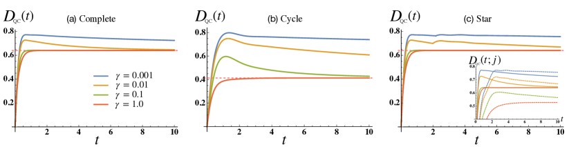
Figure 1: Quantum-classical distance computed for different values of the dephasing parameter, for different graphs with $N=5$ nodes: (a) complete graph, (b) cycle graph and (c) star graph. Dashed pink line indicate the asymptotic value $D_{\text{\tiny QC}}(t_{\infty})$ in the three considered cases. The inset of figure (c) shows the $D_{\text{\tiny QC}}(t;j)$ starting from the two different kind of nodes for the star graph: central (solid lines) and outer (dashed lines). $t$ is a dimensionless time.

At the initial time $D_{\text{\tiny QC}}(0)=0$, then the distance grows with time, and eventually reaches an horizontal asymptote, not necessarily monotonically depending on the value of $\gamma$. This asymptote does not depend on the decoherence parameter which, in turn, only affects the rate of convergence of $D_{\text{\tiny QC}}$ to its asymptotic value. In particular, as $\gamma$ gets bigger the distance converges more rapidly. For vanishing $\gamma$, the QC-distance for the noiseless case is recovered. We observe that intrinsic decoherence indeed brings the quantum walk closer to the classical random walk as the decoherence rate increases. However, due to the degeneracy of the spectrum, the QW does not become fully classical and the QC-distance remains positive at all times $t>0$. Notice that the qualitative behaviour of the QC-distance does not depend on the number of nodes $N$, i.e. a behaviour similar to that of Fig. 1 is observed for every $N$.

Let us now prove that the asymptotic value of the QC-distance does not depend on the rate $\gamma$ but rather it is a function of $N$ only. The Laplacian spectrum of an $N$-node complete graph reads $\lambda_{1}=\cdots=\lambda_{N-1}=N$ and $\lambda_{N}=0$. The corresponding eigenvectors are

$$|\lambda_{k}\rangle=\frac{1}{\sqrt{N}}\sum_{j=1}^{N}e^{i\frac{2\pi k}{N}j}|j\rangle.$$ (12)

In order to obtain the stationary quantum-evolved state in Eq.(9), we first need to find the values of $n$ and $p$ for which $\lambda_{n}=\lambda_{p}$ holds. For the complete graph this condition is satisfied when $n\neq N\wedge p\neq N$ or $n=p=N$. Hence, it follows that the stationary quantum state reads

$$\rho_{\infty}{=}\frac{1}{N}|\lambda_{N}\rangle\!\langle\lambda_{N}|+\frac{1}{N}\sum_{n,p=1}^{N-1}|\lambda_{n}\rangle\!\langle\lambda_{p}|\,,$$ (13)

where we used $\langle N|\lambda_{k}\rangle=\frac{1}{\sqrt{N}}\,\,\forall k$. We can now compute the asymptotic value of the QC-distance:

$$D_{\text{\tiny QC}}(t_{\infty})= 1-\frac{1}{N^{2}}\left(1+\sqrt{N-1}\right)^{2}.$$ (14)

Indeed the asymptotic value does not depend on the decoherence rate $\gamma$, but only on the number of nodes $N$. Notice that for $N\rightarrow\infty$ we retrieve the asymptote of the noiseless case, i.e. $1-\frac{1}{N}$. This suggests that, as the size of the complete graph grows, the effect of intrinsic decoherence becomes negligible.

3.2 Cycle Graph

The cycle graph is a one-dimensional lattice with periodic boundary conditions, i.e. it is a regular graph with vertex degrees $d_{j}=2\quad\forall j$. The Laplacian for a $N$-node cycle graph is a tridiagonal matrix with off-diagonal elements $L_{j,j+1}=L_{j+1,j}=-1$ $\forall j=1,\dots,N-1$ and diagonal elements $L_{jj}=2$ $\forall j$. As for the previous case, and without loss of generality, we choose $\rho_{j}=\outerproduct{N}{N}$ as initial localized state of the walker.

The behaviour of $D_{\text{\tiny QC}}(t)$ is qualitatively similar to the complete graph, see Fig. 1(b), i.e. intrinsic decoherence brings the quantum evolution closer to the classical one compared to the noiseless case. However, although some quantumness is lost, the degeneracy of the Laplacian’s spectrum prevents a full classicalization of the QW. Depending on the value of $\gamma$, the QC-distance may reach its asymptotic value non-monotonically, i.e. displaying a maximum at shorter times, or monotonically. We observed that, for a fixed number of nodes, the asymptotic value of $D_{\text{\tiny QC}}(t)$ is smaller with respect to the case of the complete graph.

To calculate the asymptotic value $D_{\text{\tiny QC}}(t_{\infty})$, we need $\mathcal{E}_{\infty}[\rho_{j}]$ and, in turn, the values of $n$ and $p$ that fulfill the condition $\lambda_{n}=\lambda_{p}$. The eigenvalues of the $N$-cycle graph Laplacian are $\lambda_{n}=2\left[1-\cos\left(\frac{2\pi n}{N}\right)\right]$, with $n=1,\cdots,N$, and the corresponding eigenstates coincide with those in Eq. (12). In particular, $\lambda_{n}=\lambda_{p}$ is satisfied when $n=p$ or when $n=N-p$ with $p\neq N$. In order to explicitly evaluate $D_{\text{\tiny QC}}(t_{\infty})$, we study the odd and the even $N$ cases separately, since when $N$ is even there are $\frac{N}{2}-1$ couples of equal eigevalues, while when $N$ is odd there are $\frac{N-1}{2}$ of them. With this in mind, we obtain the stationary quantum state

$$\mathcal{E}_{\infty}[\rho_{j}]=\frac{1}{N}\mathbb{I}+\frac{1}{N}\sum_{p=1}^{N-1}|\lambda_{N-p}\rangle\!\langle\lambda_{p}|$$ (15)

where $p\neq\frac{N}{2}$ if $N$ is even. After diagonalizing $\mathcal{E}_{\infty}[\rho_{j}]$, the asymptote of the QC-distance can be easily computed. When $N$ is even we obtain

$$D_{\text{\tiny QC}}(t_{\infty})=1-\frac{1}{N^{2}}\left(2+\frac{N-2}{\sqrt{2}}\right)^{2}\,,$$ (16)

while for odd $N$ we get

$$D_{\text{\tiny QC}}(t_{\infty})=1-\frac{1}{N^{2}}\left(1+\frac{N-1}{\sqrt{2}}\right)^{2}.$$ (17)

In both cases, we see that as $N\rightarrow\infty$ the asymptotic value of the QC-distance approaches $\frac{1}{2}$, as opposed to the complete graph case, where the asymptote reaches unity in the same limit, see Fig. 2 for a comparison.

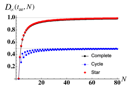
Figure 2: Asymptotic value of $D_{\text{\tiny QC}}$ in the case of intrinsic decoherence, as a function of the graph size $N$, for the complete (black dots), cycle (blue squares) and star (red rhombus) graph. The values for the complete and star graph are identical.

3.3 Star Graph

As opposed to the complete graph and the cycle graph, the nodes of a star graph are not all equivalent, but are rather grouped into two categories: the central node, which we will refer to as $|1\rangle$, and the remaining $N-1$ external nodes. Consequently, the computation of the $D_{\text{\tiny QC}}(t)$ involves an optimization over these two distinct classes of initial states, consistently with the definition in Eq. (6). Fig. 1(c) shows the QC-distance of a quantum walker moving on a star graph. Note that the points of the plot where the function is not differentiable correspond to intersections between the QC-distance of a walker initially localized in the center node and that of a walker whose initial state is an external node. We first study the system with initial state $\rho_{1}=\outerproduct{1}{1}$ and denote this distance with $D_{\text{\tiny QC}}(t,c)$, where $c$ stands for the central node. Numerical computation of the distance between the classical and the quantum noisy evolution shows that $D_{\text{\tiny QC}}(t,c)$ is the same as the one obtained for the complete graph. The same happens in the noiseless case, where analytic calculations of the quantum and classical transition probabilities for the two graphs have the same expressions Xu2009 , as long as the walker is initialized in the central vertex of the star graph. Moreover, it is possible to show numerically that the QC-distance for the complete graph is equivalent to that of a larger class of $N$-nodes graphs, namely those obtained from an $N$-dimensional complete graph by removing edges that are not connected to the central node $|1\rangle$. This holds true for the noiseless scenario razzoli22 as well as for the dynamics induced by intrinsic decoherence.
If, instead, the initial state is localized on any of the external nodes we obtain a different distance, that we call $D_{\text{\tiny QC}}(t,e)$ (see the inset of Fig 1(c)). In particular, while at short times the maximum of the $D_{\text{\tiny QC}}(t)$ is obtained by starting from the central node, at intermediate times it can be obtained by starting from one of the external nodes, depending on the value of the parameter $\gamma$. At longer times, the central node always proves to be the optimal initialization for the walker. We can indeed compute the asymptotic value of $D_{\text{\tiny QC}}(t,e)$ through Eq. (10). Given the Laplacian eigenvalues $\lambda_{1}=\cdots=\lambda_{N-2}=1$, $\lambda_{N-1}=0$ $\lambda_{N}=N$, and its respective eigenvectors Xu2009 :

$$|\lambda_{k}\rangle=\sqrt{\frac{k}{k+1}}|k+2\rangle-\sqrt{\frac{1}{k(k+1)}}\sum_{j=2}^{k+1}|j\rangle,$$ (18)

for $k=1,\cdots,N-2$ and

$$|\lambda_{N-1}\rangle=\frac{1}{\sqrt{N}}\sum_{j=1}^{N}|j\rangle$$ (19)

$$|\lambda_{N}\rangle=\frac{1}{\sqrt{N(N-1)}}\sum_{j=1}^{N}|j\rangle-\sqrt{\frac{N}{N-1}}|1\rangle,$$ (20)

one obtains the following stationary state

$$\mathcal{E}_{\infty}[\rho_{j}]= \frac{1}{N}|\lambda_{N-1}\rangle\!\langle\lambda_{N-1}|+\frac{1}{N(N-1)}|\lambda_{N}\rangle\!\langle\lambda_{N}|+$$

$$+ \sum_{j,k=1}^{N-2}\frac{1}{\sqrt{j(j+1)}}\frac{1}{\sqrt{k(k+1)}}|\lambda_{j}\rangle\!\langle\lambda_{k}|.$$ (21)

The asymptote of the QC-distance, having fixed the initial state to an external node, then reads

$$D_{\text{\tiny QC}}(t_{\infty},e)=1-\frac{\left(\sqrt{N(N-2)}+\sqrt{N-1}+1\right)^{2}}{N^{2}(N-1)}$$ (22)

which is always lower than the one obtained via the central node as initial state. Hence, the asymptotic distance

$$D_{\text{\tiny QC}}(t_{\infty}) =\max\left[D_{\text{\tiny QC}}(t_{\infty},c),D_{\text{\tiny QC}}(t_{\infty},e)\right]=D_{\text{\tiny QC}}(t_{\infty},c)$$ (23)

of the star-graph has the same expression of the asymptotic distance obtained for the complete graph, Eq. (14), as shown in Fig. 2. We can thus conclude that the quantumness of the QW is better preserved asymptotically if the walker is initially localized in the central node of the graph.

4 Decoherence in the position basis

Besides energy, the other natural basis to consider for decoherence phenomena is that of the states localized on the graph’s nodes $\{\ket{k}\}_{k=1}^{N}$. In the following, we analyze two different phenomenological models of decoherence in this basis.
We first consider the Haken-Strobl master equation introduced in Eq. (4) which, expressed in the node basis, can be recast into the following form:

$$\frac{d\rho(t)}{dt}=-i\left[L,\rho(t)\right]-\gamma(\mathbb{J}-\mathbb{I})\circ\rho(t).$$ (24)

Here $\mathbb{J}$ is the unit matrix, i.e. a matrix whose entries are all 1, $\mathbb{I}$ is the identity matrix, $\rho$ is the density matrix expressed in the node basis and $\circ$ denotes the Hadamard product of matrices (entry-wise product). Notice how the off-diagonal damping terms on the rhs of the equation do not depend on the distance between the sites. These dissipative terms cause off-diagonal elements of the density matrix to vanish asymptotically and, at the same time, they also induce a non-trivial dynamics of the diagonal elements since the commutator in the master equation, i.e. the unitary evolution, couples coherences with populations.

We have computed the QC-distance for the complete, cycle and star graphs, and for different values of the decoherence parameter $\gamma$, as in Fig. 3. Some general features of $D_{\text{\tiny QC}}(t)$ do not depend on the kind of graph at study.

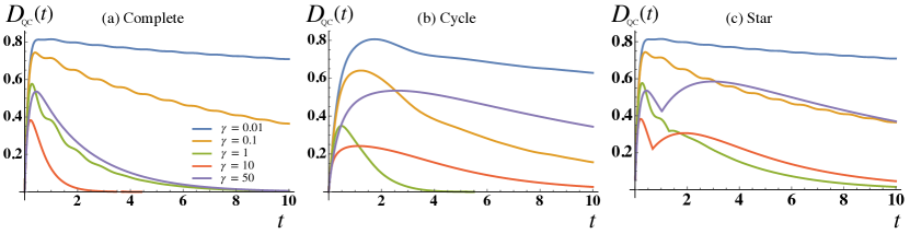
Figure 3: Quantum-classical distance for a walker subject to the Haken-Strobl decoherent dynamics described by Eq. (24) for a (a) complete (b) cycle and (c) star graph with $N=7$ nodes, computed for different values of the dephasing parameter $\gamma$.

In particular, we find that the quantum-classical distance, after overcoming one or two local maxima, goes to zero asymptotically. This in turn means that the quantum walk reaches the uniform distribution as a stationary state. Hence, contrary to the model of intrinsic decoherence in the energy basis, this map is able to suppress all quantum features of the QW and turn it into the classical random walk asymptotically. The cuspids in Fig. 3(c) corresponding to the star graph case, arise because of the maximization over classical initial states involved in the definition of $D_{\text{\tiny QC}}(t)$. In particular, for large values of $\gamma$ and at short times, the central node is the one achieving maximal QC-distance, while after the point where the function is not differentiable, the maximum is obtained by preparing the walker in any of the external nodes. On the other hand, for smaller values of $\gamma$ the maximization is achieved at all times by initializing the QW in the central node of the star graph.

Also in this case, the decoherence parameter $\gamma$ affects the speed of convergence of the QC-distance to its horizontal asymptote. However, as opposed to the intrinsic decoherence model, it is not true anymore that whenever $\gamma$ grows so does the speed of convergence of $D_{\text{\tiny QC}}$ to its asymptotic value. In fact, there is a value of $\gamma$, dependent on the dimension and on the topology of the graph, after which there is an ’inversion’ and the convergence speed starts decreasing. This fact can be intuitively understood in the asymptotic scenario $\gamma\gg 1$, where the off-diagonal elements of the density matrix experience approximately pure exponential decay, since we can neglect the unitary evolution. It is then trivial to show that, within this approximation, the system stays in the initial localized state. We thus conclude that, as $\gamma$ grows beyond a certain threshold, decoherence effects dominate over the unitary evolution and the system is frozen in the initial state. As a result it takes increasingly more time for the quantum walk to reach the uniform distribution for larger values of $\gamma$.

The second model of decoherence in the nodes basis we consider is the quantum stochastic walk, where the classical and the quantum dynamics are mixed at the master equation level via interpolation through a single real parameter $p$, see Eq. (5). We can solve this master equation numerically and compute the QC-distance for different values of the mixing parameter $p$ and for the classes of graphs we have considered in this work. Our numerical results show that this kind of noise is able to classicalize the quantum walk asymptotically, regardless of the topology of the underlying graph and for every value of $p>0$. The parameter $p$ only affects the speed of convergence of $D_{\text{\tiny QC}}(t)$ to zero, as can be seen in Fig. 4.

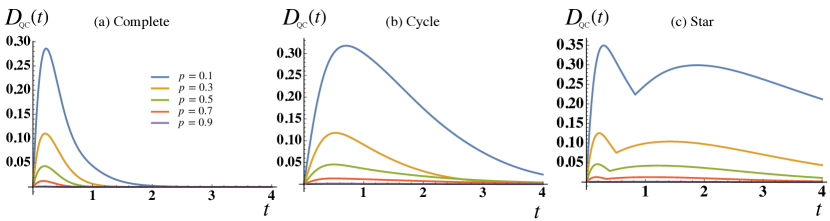
Figure 4: Quantum-classical distance for a walker subject to decoherent dynamics induced by QSW for a (a) complete (b) cycle and (c) star graph with $N=7$ nodes, computed for different values of the mixing parameter $p$.

The larger the value of $p$ the faster the QW transitions into a classical random walk, since the classical component in the dynamics has a larger weight in this case, according to Eq. (5). We point out that, contrary to the two previous models of decoherence, in this case we find that the QC-distance of a quantum walker initially localized in the central node of a star graph does not coincide with that of a quantum walk on a complete graph. The discontinuity in the QC-distance derivative in Fig. 4(c) signals a change of the initial state that satisfies the maximization condition in the definition (6). In particular, while at short times this condition is achieved by having the initial state localized in the central node, at larger times this is attained by initializing the walker to any of the external nodes. As a final remark, we want to highlight the shorter time-scale in Fig. 4 with respect to Fig. 3, indicating a faster classicalization dynamics. The QSW model appears to be the less robust to decoherence for the topologies and choice of parameters considered.

5 Conclusions

Noise is a challenge to practical realisation of quantum walks. Indeed, the presence of noise induces decoherence, and loss of quantum features, which are critical to achieve quantum advantages, i.e. to outperform protocols and algorithms based on classical random walks.

In this work, upon employing a fidelity-based measure of dynamical distance, we have addressed the effects of decoherence on CTQWs. In particular, we have investigated quantitatively the differences between the dynamics of a quantum walker in the presence of noise, and that of the corresponding classical walker on a given graph. In this way, we have been able to assess if, and to which extent, decoherence makes the quantum walker to turn into a classical incoherent random walker.

We have considered three different models of decoherence for a CTQW. We have first focused on intrinsic decoherence, i.e. decoherence in the energy eigenbasis, and linked the degeneracy of the Laplacian spectrum to the impossibility for this kind of noise to completely classicalize the quantum walker. In this case, we have analytically characterised the asymptotic behaviour of the quantum-classical distance, and discussed how the connectivity of the graph influences the speed of convergence to its asymptotic value. We have then shifted our attention towards two models of decoherence in the node basis, namely the quantum dynamics arising from the Haken-Strobl master equation, and the quantum stochastic walk model, which interpolates between the classical and quantum RW by means of a single real mixing parameter. In both cases we have shown that all quantum features of the dynamics are suppressed asymptotically, i.e. the quantum walker behaves like a classical random walker in the long-time limit.

Our analysis has shown that, at least for the considered classes of graphs, the qualitative features of the quantum-classical distance are not influenced by the topology of the graph, and by the number of its nodes. In addition, the asymptotic value of the quantum-classical distance does not depend on the relevant noise parameter. Finally, we have found that there is no universal behavior of the classicalization speed as a function of the decoherence rates. A larger decoherence corresponds to a faster convergence of the QC-distance to its asymptotic value for intrinsic decoherence and the QSW models, whereas in the Haken-Strobl scenario, larger values of the decoherence rate induce localization of the walker.

Our results contribute to deepen the knowledge on the effects of noise and decoherence on quantum walks, and pave the way to engineering of decoherence, as well as to identifying regimes where its effects may be mitigated.

Appendices

Appendix A Graph symmetries and degenerate eigenvalues

In the following we show that the survival of quantum coherences in the asymptotic quantum state Eq. (9), due to the presence of degenerate Laplacian eigenstates, can be traced back to the symmetries of the underlying graph. The symmetries of a graph $G(V,E)$ are, in turn, related to the group $\Gamma(G)$ of its automorphisms, i.e. the group of permutations $\sigma:V\rightarrow V$ of the set of vertices $V$ such that $\left(\sigma(n),\sigma(p)\right)\in E\Leftrightarrow(n,p)\in E$, $\forall n,p\in V$, i.e. adjacency is preserved. It follows, for example, that for the complete graph every permutation of the nodes identifies a symmetry while, for the star graph, only permutations of the external nodes are automorphisms. The connection between the symmetries of a graph and the degeneracy of its spectrum is provided by the following theorem merris :

Theorem: Let $G(V,E)$ be a connected graph and $\Gamma(G)$ the group of its automorphisms. If a permutation in $\Gamma(G)$ contains $s$ odd cycles and $t$ even cycles, then the Laplacian matrix will have at most $s+2t$ simple eigenvalues.

It follows that if a permutation in $\Gamma(G)$ contains a cycle with at least 3 elements, the spectrum of $L$ is degenerate and the QC-distance will not reach zero asymptotically. We stress that this is only a sufficient condition for degeneracy. This explains why the QC-distance in Eq. (10) does not reach zero for the classes of graphs studied in this paper, where it is particularly easy to find symmetries involving three or more nodes. On the other hand, we expect to witness a different behavior with other classes of graphs, such as random graphs. In this case, especially for large values of $N$, it is likely that the only symmetries of the graph will be permutations decomposable in cycles of 1 and 2 nodes only. Consequently, in this situation the theorem only tells us that $L$ will have at most $N$ simple eigenvalues, hence it is of no help.

References

- (1) J. Kempe, Quantum random walks: An introductory overview, Contemp. Phys. 44(4), 307 (2003)
- (2) S.E. Venegas-Andraca, Quantum walks: a comprehensive review, Quant. Inf. Process. 11(5), 1015 (2012)
- (3) F. Xia, J. Liu, H. Nie, Y. Fu, L. Wan, X. Kong, Random walks: A review of algorithms and applications, IEEE Trans. Emerg. Top. Comput. Intell. 4(2), 95 (2020). DOI 10.1109/TETCI.2019.2952908
- (4) K. Kadian, S. Garhwal, A. Kumar, Quantum walk and its application domains: A systematic review, Comput. Sci. Rev. 41, 100419 (2021)
- (5) M. Frigerio, C. Benedetti, S. Olivares, M.G.A. Paris, Generalized quantum-classical correspondence for random walks on graphs, Phys. Rev. A 104, L030201 (2021)
- (6) Y. Aharonov, L. Davidovich, N. Zagury, Quantum random walks, Phys. Rev. A 48, 1687 (1993)
- (7) E. Farhi, S. Gutmann, Quantum computation and decision trees, Phys. Rev. A 58, 915 (1998)
- (8) O. Mülken, A. Blumen, Continuous-time quantum walks: Models for coherent transport on complex networks, Phys. Rep. 502(2-3), 37 (2011)
- (9) O. Mülken, V. Pernice, A. Blumen, Quantum transport on small-world networks: A continuous-time quantum walk approach, Phys. Rev. E 76, 051125 (2007)
- (10) L. Razzoli, M.G.A. Paris, P. Bordone, Transport efficiency of continuous-time quantum walks on graphs, Entropy 23(1), 85 (2021)
- (11) M. Maciel Cássio, C.F.O. Mendes, W.T. Strunz, M. Galiceanu, Quantum transport on generalized scale-free networks, Phys. Rev. A 102, 032219 (2020)
- (12) A. Ambainis, Quantum walks and their algorithmic applications, Int. J. Quantum Inf. 1(04), 507 (2003)
- (13) R. Portugal, Quantum Walks and Search Algorithms (Springer International Publishing, 2018)
- (14) A.M. Childs, Universal computation by quantum walk, Phys. Rev. Lett. 102, 180501 (2009)
- (15) K. Wang, Y. Shi, L. Xiao, J. Wang, Y.N. Joglekar, P. Xue, Experimental realization of continuous-time quantum walks on directed graphs and their application in pagerank, Optica 7(11), 1524 (2020)
- (16) R. Herrman, T.G. Wong, Simplifying continuous-time quantum walks on dynamic graphs, Quantum Inf. Process. 21(2), 54 (2022)
- (17) N. Inui, K. Kasahara, Y. Konishi, N. Konno, evolution of continuous-time quantum random walks on circles, Fluct. Noise Lett. 05(01), L73 (2005)
- (18) M.B. Plenio, S.F. Huelga, Dephasing-assisted transport: quantum networks and biomolecules, New J. Phys. 10(11), 113019 (2008)
- (19) F. Caruso, A.W. Chin, A. Datta, S.F. Huelga, M.B. Plenio, Highly efficient energy excitation transfer in light-harvesting complexes: The fundamental role of noise-assisted transport, J. Chem. Phys. 131(10), 105106 (2009)
- (20) A. Schreiber, K.N. Cassemiro, V. Potoček, A. Gábris, I. Jex, C. Silberhorn, Decoherence and disorder in quantum walks: From ballistic spread to localization, Phys. Rev. Lett. 106, 180403 (2011)
- (21) C. Benedetti, F. Buscemi, P. Bordone, M.G.A. Paris, Non-markovian continuous-time quantum walks on lattices with dynamical noise, Phys. Rev. A 93, 042313 (2016)
- (22) D. Tamascelli, A. Segati, S. Olivares, Dephasing assisted transport on a biomimetic ring structure, Int. J. Quant. Inf. 15(08), 1740006 (2017)
- (23) C. Benedetti, M.A.C. Rossi, M.G.A. Paris, Continuous-time quantum walks on dynamical percolation graphs, Europhys. Lett. 124(6), 60001 (2019)
- (24) A. Kurt, M.A.C. Rossi, J. Piilo, Efficient quantum transport in a multi-site system combining classical noise and quantum baths, New J. Phys. 22(1), 013028 (2020)
- (25) V. Gualtieri, C. Benedetti, M.G.A. Paris, Quantum-classical dynamical distance and quantumness of quantum walks, Phys. Rev. A 102, 012201 (2020)
- (26) M. Frigerio, C. Benedetti, S. Olivares, M.G.A. Paris, Quantum-classical distance as a tool to design optimal chiral quantum walks, Phys. Rev. A 105, 032425 (2022)
- (27) G.J. Milburn, Intrinsic decoherence in quantum mechanics, Phys. Rev. A 44, 5401 (1991)
- (28) H. Haken, G. Strobl, An exact solvable model for coherent and incoherent excitation motion, Z. Phys. 262, 135 (1973)
- (29) J.D. Whitfield, C.A. Rodríguez-Rosario, A. Aspuru-Guzik, Quantum stochastic walks: A generalization of classical random walks and quantum walks, Phys. Rev. A 81, 022323 (2010)
- (30) B. Nica, A brief introduction to spectral graph theory (EMS Textbooks in Mathematics, 2018)
- (31) T.G. Wong, L. Tarrataca, N. Nahimov, Laplacian versus adjacency matrix in quantum walk search, Quantum Inf. Proc. 15(10), 4029 (2016)
- (32) A. Candeloro, L. Razzoli, S. Cavazzoni, P. Bordone, M.G.A. Paris, Continuous-time quantum walks in the presence of a quadratic perturbation, Phys. Rev. A 102, 042214 (2020)
- (33) P. Rebentrost, M. Mohseni, I. Kassal, S. Lloyd, A. Aspuru-Guzik, Environment-assisted quantum transport, New J. Phys. 11, 033003 (2009)
- (34) F. Caruso, Universally optimal noisy quantum walks on complex networks, New J. Phys. 16 (2014)
- (35) X.P. Xu, Exact analytical results for quantum walks on star graphs, J. Phys. A Math. Theor. 42(11), 115205 (2009)
- (36) L. Razzoli, P. Bordone, M.G.A. Paris, Universality of the fully connected vertex in laplacian continuous-time quantum walk problems, arXiv:2202.13824 (2022)
- (37) R. Merris, Laplacian matrices of graphs: a survey, Linear Algebra Appl. 197-198, 143 (1994)