A Cosmological Lithium Solution from Discrete Gauged Baryon Minus Lepton Number

Abstract

The cosmological lithium problem—that theory predicts a primordial abundance far higher than the observed value—has resisted decades of attempts by cosmologists, nuclear physicists, and astronomers alike to root out systematics. We reconsider this problem in the setting of the Standard Model extended by gauged baryon minus lepton number, which we spontaneously break by a scalar with charge $2N_{c}N_{g}$. Cosmic strings from this breaking can support interactions converting three protons into three positrons, and we argue that an ‘electric’-‘magnetic’ interplay can give this process an amplified, strong-scale cross-section in an analogue of the Callan-Rubakov effect. We suggest such cosmic strings have disintegrated $\mathcal{O}(1)$ of the primordial lithium nuclei, and lay out what is necessary for this scheme to succeed. To our knowledge this is the first new physics mechanism with microphysical justification for the abundance of lithium uniquely to be modified after Big Bang Nucleosynthesis.

Figure 0: Photo of a commissioned abstract artist’s impression in acrylic on canvas by Bailey Lingen, a Chicago-based artist and trans rights activist who produces music under the name LiTHiUM THiEF.

 

1 The Lithium Problem

	$\left({}^{7}\text{Li}/\text{H}\right)$
Observation	$\left(1.6\pm 0.3\right)\times 10^{-10}$
Theory	$\left(4.7\pm 0.7\right)\times 10^{-10}$

Table 1: For reference, the status of the number density of lithium-7 relative to that of hydrogen, taken from the recent review and status update Fields:2019pfx .

Big Bang Nucleosynthesis (BBN) is the theory of the formation of light nuclei a few minutes after the hot big bang, and is the earliest epoch of the universe for which we have direct evidence. In the framework of the Standard Models (SM) of particle physics and cosmology, BBN is essentially a parameter-free cross-check on our understanding of the universe. And a powerful one at that: BBN is sensitive to all four known forces, as it pits the strong force’s ability to bind nucleons against the gravitational expansion of the universe, the weak decays of the neutron, and the electromagnetic repulsion of protons. The status is given by the comparison of theoretical predictions and empirical observations of just three quantities Fields:2019pfx ; Iocco:2009a ; Coc:2017pxv ; Mathews:2017xht : The primordial abundances of deuterium with one proton, of helium-4 with two protons, and of lithium-7 with three protons. It’s these three values that characterize our only semi-direct understanding of the universe far before recombination.

While theory and observation agree well for hydrogen and helium, there has been a consistent mystery regarding the abundance of lithium Fields:2011 ; Iocco:2012a beginning with observations in 1982 by Spite and Spite Spite:1982a ; Spite:1982b , and the current best values are shown in Table 1. The concern, of course, is what sort of systematic effects might be responsible. Early on there was a possibility of unseen effects in the nuclear data Cyburt:2009cf , but the relevant transition rates are thought to have now all been measured, with by 2015 a status update stating “a ‘nuclear option’ to the lithium problem is essentially excluded” Cyburt:2008kw ; Cyburt:2015mya ; Iliadis:2020a . Continued measurement and modelling has agreed Pitrou:2018cgg ; Rijal:2019a ; nTOF:2018vnr ; Bystritsky:2017a and ever-more-inventive channels are being studied by nuclear physicists and discarded as inconsequential Voronchev:2009zz ; Kirsebom:2011vp ; Li:2018a ; Hartos:2018tpy ; Damone:2018a .

The remaining worry arises since the empirical data on ‘primordial’ lithium comes primarily from measurements of its abundance in the atmospheres of metal-poor, population II stars in the Milky Way. While we must necessarily use nearby sources due to the scarcity of lithium, the argument that we can access the primordial abundance follows from elementary stellar dynamics considerations and was given by Spite & Spite Spite:1982a ; Spite:1982b . In relatively cool stars, the full volume of the star undergoes convection, such that lithium from the atmosphere may be convected to the core and destroyed. However, hot-enough stars develop an inner radiative zone which is convectively stable, such that convection is confined to an outer layer and the lithium abundance in the atmosphere does not get reprocessed. Then if one measured the lithium abundance in atmospheres of stars whose lithium is primordial, as a function of temperature—with all of the proper astronomical care taken to look at the right sorts of stars—for cooler stars there should be less and less of it, but on the other side at some temperature the plot should level off to a constant value. Indeed, this is the famous ‘Spite plateau’ which was observed first by Spite and Spite in 1982 Spite:1982a ; Spite:1982b , suggesting that this plateau abundance indeed grants us an observational window to the primordial abundance. The next few decades of observational progress (e.g. Rebolo:1988a ; Balachandran:1990a ; Ryan:1996a ; Ryan:1998a ; Ryan:1999a ; Boesgaard:2005a ; Charbonnel:2005a ; Bonifacio:2006au ; Asplund:2006a ; Aoki:2009a ; Hosford:2009a ; Sbordone:2010a ; Schaeuble:2012a ) in measuring stellar lithium are reviewed in Spite:2012 , overall showing further support for a Spite plateau discrepant with the BBN predictions. This has now included observations of the Spite plateau in environments as diverse as stellar streams Aguado:2021a , multiple globular clusters Bonifacio:2002a ; Mucciarelli:2011a ; Schiappacasse-Ulloa:2022 , the Sculptor dwarf spheroidal galaxy Hill:2019a , the Gaia-Enceladus galaxy Molaro:2020a ; Simpson:2021a , and Messier 54 Mucciarelli:2014a . A recent study of galactic chemical evolution models for these data concluded that the observed abundances were well-understood only if the primordial lithium abundance was set to the Spite plateau value Matteucci:2021 .

In recent years some ever-larger datasets have showed slightly higher variability Bonifacio:2006au ; Bonifacio:2007a ; Gonzalez:2009a ; Monaco:2012a ; Crandall:2014cca ; Melendez:2010a ; Howk:2012a in the pleateau star abundances and even some anomalously low abundances in extremely metal-poor stars Sbordone:2010a ; Bonifacio:2015top , which has raised doubts in some quarters (see e.g. Deal:2021a ), but the implications of these new data are unclear Aguado:2019bac ; Matteucci:2021 and the situation is still under active investigation by many scientists in a wide variety of fields across physics and astronomy. On the theoretical side, there is no well-accepted new stellar dynamics mechanism that could be responsible, though there have been proposals Richard:2005a ; Piau:2006a ; Korn:2006a ; Prantzos:2012a ; Ouyed:2013a ; Marrder:2020a ; Tognelli:2020a ; Grisoni:2019a . On the observational side, astronomers continue to further probe the Spite plateau in a variety of innovative directions Prodanovic:2004a ; Ruchti:2011a ; Caffau:2011a ; Mucciarelli:2012 ; Hansen:2014a ; Spite:2015 ; Fu:2018a ; Bensby:2018a ; Lambert:2004a ; Pinto:2021a .

Of course, any time there is an astronomical or cosmological anomaly our Bayesian priors should be peaked toward learning something new about stars. But after so long with the prospects for an astrophysical resolution still unclear, some broader exploration is surely well worth doing. And indeed, there have been some new physics mechanisms explored—mainly fundamental constants varying to modify early-universe nuclear rates Dent:2007a ; Dmitriev:2004a ; Flambaum:2008a ; Berengut:2010a ; Cheoun:2011yn ; Landau:2006a ; Coc:2007a ; Mori:2019a ; Franchino-Vinas:2021nsf ; Clara:2020efx ; Fung:2021wbz or decaying dark matter disrupting reactions Pospelov:2006sc ; Jedamzik:2007cp ; Ellis:2005ii ; Olive:2012hig ; Coc:2014gia ; Yamazaki:2017uvc ; Cyburt:2006a ; Kaplinghat:2006a ; Bird:2008a ; Kohri:2007a ; Kusakabe:2010a ; Kusakabe:2011a ; Anchordoqui:2020djl ; Alcaniz:2019kah ; Sato:2016len ; Cyburt:2013fda ; Goudelis:2015wpa ; Pospelov:2010cw ; Bailly:2008yy ; Cumberbatch:2007me ; Jedamzik:2005dh ; Cyburt:2012kp ; Jittoh:2011ni ; Kawasaki:2010yh ; Kusakabe:2017brd ; Kusakabe:2014ola . See also Mathews:2019hbi ; Luo:2019a ; Makki:2019a ; Malaney:1993a ; Mathews:2005a ; Hou:2017a ; Nakamura:2017a ; Lu:2022a ; Flambaum:2018ohm ; Pospelov:2012pa ; Bailly:2010hh ; Cyburt:2010vz ; Olive:2012xf ; Coc:2013a ; Pospelov:2010hj for further ideas. In our diagnosis, these approaches have been stymied by not uniquely picking out lithium to be affected, and they generally encounter severe difficulties with putting other observables into tension.

We are motivated by the surprisingly long lifetime of the proton and its exact stability in the SM to take advantage of the exact SM selection rule

$$\hskip 28.45274pt\Delta(\#\text{ of baryons}) =\Delta(\#\text{ of leptons})$$

$$=0\ (\text{mod number of generations}).$$

Since the SM has $N_{g}=3$ generations of particles and the BBN predictions first fail for lithium with three protons, this symmetry could explain why elements with one or two protons are unaffected. This allows us to construct—to our knowledge—the first new physics mechanism for the lithium abundance to be discrepant which does not require tuning to avoid modifying the abundances of other elements.

We must go only slightly beyond the SM to find our effect of interest. In brief, we will break gauged baryon minus lepton number to a discrete subgroup which will produce a large abundance of cosmic string loops. These topological defects amplify the $B+N_{c}L$ violation, and we introduce a model in which leptoquarks communicate this violation in a way which picks out solely processes in which three protons are turned into three positrons. We propose that such cosmic strings have disintegrated lithium nuclei in the early universe, reducing the primordial abundance to the level inferred from astronomical observations. In this Letter we will put together the various pieces of field theory and cosmology behind this mechanism, and estimate the rate to demonstrate its plausibility. Precise predictions will require much further work.

2 Schema

	$\quad Q\quad$	$\quad\bar{u}\quad$	$\quad\bar{d}\quad$	$\quad L\quad$	$\quad\bar{e}\quad$	$\quad\bar{\nu}\quad$
$SU(3)_{C}$	$3$	$\bar{3}$	$\bar{3}$	–	–	–
$SU(2)_{L}$	$2$	–	–	$2$	–	–
$U(1)_{Y}$	$+1$	$-4$	$+2$	$-3$	$+6$	–
$U(1)_{B}$	$+1$	$-1$	$-1$	–	–	–
$U(1)_{L}$	–	–	–	$+1$	$-1$	$-1$

Table 2: Representations of the left-handed SM Weyl fermions (and the sterile neutrino) under the classical symmetries of the SM.

New physics setting

We extend the Standard Model by gauging $U(1)_{B-N_{c}L}$, which is the continuous, generation-independent, Adler-Bell-Jackiw (ABJ) Adler:1969gk ; Bell:1969ts anomaly-free ‘accidental’ global symmetry of the SM. The fermion charges are given in Table 2. We address the ’t Hooft anomaly tHooft:1979rat and neutrino oscillations by adding right-handed neutrinos, but this choice does not impact our mechanism. Though note that $U(1)_{B-N_{c}L}$ does forbid Majorana masses for neutrinos. To Higgs this gauge symmetry we introduce a scalar $\Phi$ with

$$\left[\Phi\right]_{B-N_{c}L}=2N_{c}{N_{g}},\qquad\left[\Phi\right]_{B+N_{c}L}=0,\qquad\langle\Phi\rangle=v,$$ (1)

which condenses in the early universe at a temperature $T_{c}\sim v$. This breaks the baryon minus lepton number symmetry without breaking the additional discrete anomaly-free global $\mathbb{Z}^{L}_{{N_{g}}}$ subgroup of lepton number enjoyed by the SM Koren:2022bam . The global symmetry-breaking pattern providing selection rules is

$$U(1)_{B-N_{c}L}\times\mathbb{Z}^{L}_{{N_{g}}}\rightarrow\mathbb{Z}_{2N_{c}{N_{g}}}^{B-N_{c}L}\times\mathbb{Z}^{L}_{{N_{g}}}\supset\mathbb{Z}_{2N_{c}{N_{g}}}^{B+N_{c}L},$$ (2)

where the anomaly-free subgroup of baryon plus lepton number is generated by $(1,1)\in\mathbb{Z}_{2N_{c}{N_{g}}}^{B-N_{c}L}\times\mathbb{Z}^{L}_{{N_{g}}}$. We emphasize that only the former factor is gauged in our model, though it would be interesting to consider a model in which the discrete lepton number is gauged as well. While this Higgsing is ‘non-minimal’ in the sense that $\left[\Phi\right]>1$, this choice of $\left[\Phi\right]$ preserves the SM selection rule which stabilizes the proton Tong:2017oea ; Koren:2022bam ; Anber:2021upc ; Davighi:2022qgb ; Wang:2022eag . That is, the SM constraint of $\Delta B/N_{c}=\Delta L=N_{g}$, already familiar from electroweak sphaleron processes, will remain exact in our theory.

Discrete gauge theory

The nontrivial Higgs charge $\left[\Phi\right]_{B-N_{c}L}$ means its condensation preserves an unbroken discrete $\mathbb{Z}_{2N_{c}{N_{g}}}^{B-N_{c}L}$ gauge symmetry Krauss:1988zc ; Alford:1989ch ; Preskill:1990bm ; Coleman:1991ku ; Banks:1989ag and stable cosmic string solutions exist with tension $\mu\sim v^{2}$. The transverse slices of a static, $z$-independent string are Abrikosov-Nielsen-Olesen vortices Abrikosov:1956sx ; Nielsen:1973cs and have asymptotics

$$\Phi(\rho,\theta)\rightarrow ve^{ik\theta},\qquad\vec{A}(\rho,\theta)\rightarrow\frac{k}{g}\frac{1}{2{N_{g}}}\frac{\hat{\theta}}{\rho},$$ (3)

with $\vec{A}$ the $B-N_{c}L$ gauge boson, $g$ the $U(1)_{B-N_{c}L}$ ‘electric’ charge, and $k\in\mathbb{Z}$ the winding number of $\Phi$. With nonzero winding, continuity in the interior demands a zero in the Higgs field, and indeed the $B-N_{c}L$ symmetry is unbroken in a string ‘core’ of radius $R\sim v^{-1}$. These solutions have discrete $U(1)_{B-N_{c}L}$ ‘magnetic’ fluxes

$$\Phi_{B}=\frac{2\pi}{g}\frac{k}{2N_{c}{N_{g}}}$$ (4)

confined to their cores. This magnetic flux is in ‘fractional’ units of $1/(2N_{c}{N_{g}})$ that of the Dirac magnetic flux quantum $\Phi_{0}=2\pi/g$ Dirac:1931kp , so the string is stable and interacts via the Aharonov-Bohm (AB) effect Aharonov:1959fk ; Aharonov:1984zza for the unbroken discrete symmetry. The cosmic strings undergo elastic AB scattering with all the SM fermions of differential cross-section per unit length (for a plane wave of $B-N_{c}L$ charge $q$ and momentum $p$ incident on a string) Alford:1988sj

$$\frac{1}{\ell}\frac{d\sigma}{d\theta}=\frac{\sin^{2}(\pi q\Phi_{B}/\Phi_{0})}{2\pi p\sin^{2}(\theta/2)},$$ (5)

which, importantly for the phenomenology, is independent of any high scales or small couplings.

Strings in cosmology

During an early universe phase transition, topological defects are produced proportional to the correlation length $\xi$ of the order parameter fluctuations. Causality ensures this is no larger than the Hubble distance $\xi\lesssim d_{h}$, so that at a critical temperature $T_{c}\sim v$, $\mathcal{O}(1)$ horizon-crossing strings of length $d_{h}=2H^{-1}(T_{c})\sim M_{\text{pl}}/v^{2}=(G\mu)^{-1}\ell_{pl}$ per Hubble volume are formed Kibble:1976sj ; Kibble:1980mv , $d_{h}$ being the Hubble size, $H$ the Hubble parameter, and $G\mu\sim v^{2}/M_{\text{pl}}^{2}$ a dimensionless measure of the gravitational effects of the strings. At formation, these long strings contain energy density

$$\rho_{string}\sim\frac{\mu d_{h}}{d_{h}^{3}}\sim(G\mu)^{+1}\rho_{tot},$$ (6)

a small fraction of the total. The elastic AB scattering with the SM plasma provides a total transverse cross-section per unit length of $\sigma_{\perp}/\ell\sim 1/T$, which leads to a long epoch of friction-dominated evolution until the temperature drops below $T_{f}\lesssim v^{2}/M_{\text{pl}}$ Vilenkin:1991zk .

When cosmic strings encounter each other, they ‘intercommute’ with probability approaching unity Manton:1981mp ; Shellard:1987bv ; Matzner:1988qqj ; Ruback:1988ba ; Shellard:1988ki ; Atiyah:1985dv ; Gibbons:1986df ; Rosenzweig:1990ea ; Samols:1991ne ; Abdelwahid:1993fg ; MacKenzie:1995np ; Gauntlett:2000ks ; Hanany:2005bc ; Hashimoto:2005hi . This results in the production of small-scale structure on the strings Blanco-Pillado:2015ana ; Kibble:1990ym ; Copeland:2009dk ; Kibble:1990ym ; Siemens:2001dx ; Siemens:2002dj and many closed loops from strings crossing themselves. String loops oscillate and shrink via gravitational radiation Vilenkin:1981kz ; Vilenkin:1981bx ; Vilenkin:2000jqa , which dissipates energy and prevents the strings from dominating the density budget Turok:1984db .

After decades, we now understand the behavior of the cosmic string network at late times and on large scales: There is an attractor ‘scaling’ solution where the length spectrum of loops depends only on the ratio with the horizon distance $\ell/d_{h}$ Albrecht:1984xv ; Bennett:1987vf ; Shellard:1987bv ; Shellard:1988zx ; Matzner:1988qqj ; Moriarty:1988em ; Myers:1991yh . The small scale behavior of this ‘scaling’ population is assumed to continue down to the ‘gravitational cutoff’ scale $\ell\sim(G\mu)d_{h}$, at which length a loop evaporates within a Hubble time, which leads to a large number of ‘small’ such loops, $n\sim(G\mu)^{-0.7}$ Blanco-Pillado:2013qja .

However, the regime relevant for their effects on lithium requires understanding cosmic strings far before the infrared fixed point is reached. In addition to being very difficult to study, this is sensitive to details such as the strength of the phase transition, since the correlation length of Higgs fluctuations may in fact be quite small compared to the horizon length $\xi\ll d_{h}$, resulting in a far greater initial number density of defects Guth:1982pn ; Zurek:1985qw ; Murayama:2009nj . The small-scale behavior is also sensitive to the details of intercommutation dynamics, and furthermore the presence of currents on the strings may stabilize them against decay and result in a large portion of energy density in cosmic string ‘vortons’ Davis:1988ij ; Brandenberger:1996zp ; Davis:1996zg ; Carter:1999an ; Peter:2013jj ; Auclair:2020wse ; Battye:2021kbd . For these reasons, rather than attempting to model the evolution of the phase space of cosmic strings, below we will simply parametrize their effects on lithium disintegration in terms of the fraction of the energy density which is in cosmic strings.

	$\quad\Phi\quad$	$\quad\chi\quad$	$\quad\omega_{\ell}\quad$	$\quad\omega_{q}\quad$	$\quad\omega_{s}\quad$
$SU(3)_{C}$	–	–	$3$	$3$	–
$SU(2)_{L}$	–	–	–	–	–
$U(1)_{Y}$	–	–	$-8$	$-8$	–
$U(1)_{B}$	$+9$	$+9$	$+1$	$-2$	$+3$
$U(1)_{L}$	$-3$	$+3$	$+1$	$0$	$+1$

Table 3: Representations of the scalars added in our benchmark model. Cosmic strings appear from the winding of $\Phi$ in the vacuum, the condensation of $\chi$ on the string allows it to freely exchange $B+N_{c}L$, and the scalars $\omega$ communicate $B+N_{c}L$-breaking by $\chi$ to the right-handed SM fields.

Topological defect catalysis

We wish to consider interactions which destroy lithium nuclei by turning three protons into three positrons, thereby violating $B+N_{c}L$ by $2N_{c}{N_{g}}$ units. We utilize a stringy analogue of the Callan-Rubakov effect where grand unified monopoles ‘catalyze’ proton decay at strong scale rates $\sigma(p^{+}+\text{ monopole}\rightarrow e^{+}+\text{ monopole})\sim\Lambda_{\text{QCD}}^{-2}$. For monopoles, the inevitability of such inelastic interactions can be seen purely from the infrared Dirac:1931kp ; Dirac:1948um ; Goldhaber:1965cxe ; Weinberg:1965rz ; Zwanziger:1968ams ; Peres:1968umt ; Lipkin:1969ck ; Wu:1976qk ; Schwinger:1966nj ; Zwanziger:1968rs ; Zwanziger:1970hk ; Zwanziger:1972sx ; Kazama:1976fm ; Callan:1983ed ; Csaki:2020inw ; Csaki:2020yei . An ultraviolet description for the monopole tHooft:1974kcl ; Polyakov:1974ek ; Arafune:1974uy ; Prasad:1975kr ; Julia:1975ff ; Hasenfratz:1976vb ; Tomboulis:1975qt ; Callan:1975yy ; Boulware:1976tv allows one to resolve the microphysical interactions and see $p^{+}\rightarrow e^{+}$ arising from interactions with leptoquarks in the core and the anomalous violation of $B+N_{c}L$ Jackiw:1975fn ; Hasenfratz:1976gr ; Goldhaber:1976dp ; Goldhaber:1977xw ; Callan:1982ac ; Rubakov:1981rg ; Rubakov:1982fp ; Callan:1982ac ; Callan:1982au ; Callan:1982ah ; Callan:1983tm ; Dawson:1983cm ; Sen:1984qe ; Polchinski:1984uw ; Isler:1987xn ; Rubakov:1988aq ; Affleck:1993np ; Brennan:2021ewu ; Brennan:2021ucy ; Csaki:2021ozp .

The cosmic string case has seen far less study, and no infrared argument for this catalysis effect is yet known. To provide an explicit benchmark—and to give a microphysical model targeting this mechanism toward the cosmological lithium problem—we introduce ultraviolet physics which lets us map our case on to a model studied by Alford, March-Russell, & Wilczek in 1989 Alford:1989ie in which a leptoquark condenses inside cosmic strings of some broken gauged $\widetilde{U(1)}\rightarrow\mathbb{Z}_{N}$. In that model the leptoquark allows $p^{+}\rightarrow e^{+}$ violation of $B+N_{c}L$, but here we respect the exact SM symmetry $\mathbb{Z}_{N_{g}}^{L}$, so rather than the condensation of a leptoquark we instead introduce a gauge-singlet scalar $\chi$ with

$$\left[\chi\right]_{B-N_{c}L}=0,\qquad\left[\chi\right]_{B+N_{c}L}=2N_{c}{N_{g}},\qquad\langle\chi\rangle=0,$$ (7)

but which condenses on the string core so long as

$$\left.\partial_{\chi}^{2}V(\Phi,\chi)\right|_{\Phi=0}<0\rightarrow\langle\chi\rangle_{\Phi=0}=v_{\chi}.$$ (8)

This breaks solely the global approximate $U(1)_{B+N_{c}L}$ on the string core down to the subgroup preserved by the SM, and we take the symmetry-breaking scales equal for simplicity, $\langle\Phi\rangle=v$ around the vacuum and $\langle\chi\rangle_{\Phi=0}=v$ in the string. This condensate realizes a global baryon plus lepton number analogue of Witten’s bosonic superconductivity Witten:1984eb , which allows the string core to exchange $2N_{c}{N_{g}}$ units of $B+N_{c}L$ charge with the outside world Witten:1984eb .

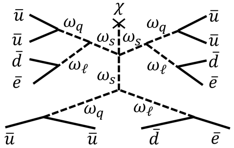
Figure 1: A Feynman diagram portraying our benchmark for how the $B+N_{c}L$-breaking effects of the $\chi$ vev get communicated to the SM fermions at low energies.

The infrared symmetries forbid interactions of $\chi$ with fewer than twelve SM fermions, but we can explicitly generate one such interaction by introducing the scalar leptoquark $\omega_{\ell}$ with hypercharge $8$ and its analogue diquark $\omega_{q}$, as well as the gauge singlet scalar $\omega_{s}$ with $B=N_{c}L=3$. This choice of scalars (see Table 3) allows the nontrivial interactions

$$\mathcal{L}\supset\lambda_{\ell}\omega_{\ell}\bar{d}\bar{e}+\lambda_{q}\omega_{q}^{\dagger}\bar{u}\bar{u}+\kappa\omega_{\ell}^{\dagger}\omega_{q}\omega_{s}+\lambda_{\chi}\omega_{s}^{3}\chi^{\dagger}.$$ (9)

Around the vacuum the Feynman diagram portrayed in Figure 1 generates the operator

$$\mathcal{L}\sim\frac{1}{v^{15}}\mathcal{\chi}(\bar{u}\bar{u}\bar{d}\bar{e})^{3},$$ (10)

and $B+N_{c}L$-violation on the string core is communicated only to electrons and protons in our model. This appears naturally due to our choice of leptoquark representations, but it would be interesting to consider relaxing this and examining the possibility of interactions with helium as well. We further take the mediators $\omega$ to be light in the string core, so this suppression by $v$ disappears when the SM fermions are interacting with the $\chi$ vev in the core, and we’ve set all couplings to unity and scales equal for simplicity.

In the model of Alford, March-Russell, & Wilczek Alford:1989ie , the Yukawa interaction allows an incoming quark to inelastically scatter into a lepton by exciting the leptoquark condensate, and the $\mathbb{Z}_{N}$ discrete gauge field background enhances the cross-section. When the discrete gauge charge of the incoming quark is maximal, the cross-section is unsuppressed by ultraviolet scales, as in the Callan-Rubakov effect. In our case, we instead have an interaction of many SM partons with the string condensate.

However, in the cosmological case of interest, a ${}^{7}\text{Li}$ nucleus delivers a state of three protons $\psi_{3p}\sim(\bar{u}\bar{u}\bar{d})^{3}$ incident upon the string. To map our model to Alford:1989ie , we rewrite Equation 10 as a Yukawa interaction between $\psi_{3p}$, the nine quarks in three protons, and $\psi_{3e}$, the three positrons. Adapting their results while ignoring many subtleties about this matching, we infer that an incoming plane wave of $B-N_{c}L$-charge $q$ and momentum $p$ undergoes enhanced inelastic scattering with a long cosmic string as

$$\frac{\sigma}{\ell}\sim\frac{1}{p}\sin^{2}\left(\pi\alpha\right)\left(\frac{p}{v}\right)^{4\left|\alpha-\frac{1}{2}\right|},\qquad\alpha\equiv\frac{kq}{2N_{c}{N_{g}}},$$ (11)

where we are generalizing Eqns 18-21 of Alford:1989ie . The inelastic scattering is unsuppressed by ultraviolet scales for an incoming state with $B-N_{c}L$ charge $q=N_{c}{N_{g}}$ in the case of a single-winding string. We note also that topological defect interactions can violate crossing symmetry, as may be understood simply for monopoles Csaki:2020inw , so for example crossing one proton to an outgoing antiproton results in a drastically suppressed cross-section because the incoming state no longer has maximal $\mathbb{Z}_{2N_{g}N_{c}}$ charge nor half-integer spin, which is also crucial for catalysis Alford:1989ie . This suppression is useful for ensuring consistency with observations of primordial helium, and it would be interesting to understand precisely the subleading rate at which helium might be affected.

Parameter space

In the early universe after BBN, just such a $q=N_{c}{N_{g}}$ state of three protons may be delivered to the string within the nuclear potential well of ${}^{7}\text{Li}$. We assume string loops have a cross-section per unit length

$$\frac{\sigma}{\ell}\left(3p^{+}+\text{ string}\rightarrow 3e^{+}+\text{ string}\right)\sim\Lambda_{\text{QCD}}^{-1},$$ (12)

but note again that there are necessarily large theoretical uncertainties here.

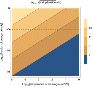
Figure 2: A contour plot of the string tension scale required for $\mathcal{O}(1)$ lithium to be disintegrated as a function of the temperature and the fraction of energy density in cosmic strings from Equation 14. The hatched region is constrained in simple models of gauged $B-N_{c}L$ with a massive $Z^{\prime}$, taking $\sqrt{\mu}\sim v\sim m_{Z^{\prime}}/g>100\text{ GeV}$ as a benchmark Heeck:2014zfa . The dashed line is an approximate upper bound on the energy density in strings near the Hubble length from CMB and gravitational wave constraints Sanidas:2012ee ; Rybak:2021scp .

However a first question is just whether such interactions can plausibly destroy an order-one fraction of lithium nuclei after BBN. Due to the complications discussed above, we will not attempt to model the evolution of the phase space of string loops, but instead content ourselves to parametrize their effects as a function of the fraction of energy density in cosmic strings. We simply ask that the rate for a lithium nucleus to encounter a cosmic string be greater than Hubble,

$$\Gamma\simeq\int d\ell\frac{dn}{d\ell}\sigma\simeq\Lambda_{\text{QCD}}^{-1}\int d\ell\frac{dn}{d\ell}\ell=\frac{\rho_{\text{string}}}{\Lambda_{\text{QCD}}\mu}\gtrsim H,$$ (13)

where we have begun with a general differential number density of cosmic strings $\frac{dn}{d\ell}$, and assumed the interaction is characterized as $\sigma/\ell=\Lambda_{\text{QCD}}^{-1}$ which makes the rate proportional to the energy density. Then introducing $f\equiv\rho_{\rm string}/\rho_{\rm tot}$ we require

$$f\gtrsim\frac{\Lambda_{\rm QCD}}{M_{\rm pl}}\frac{\mu}{T_{\star}^{2}},$$ (14)

where $\Lambda_{\rm QCD}/M_{\rm pl}\sim 10^{-20}$, and $T_{\star}$ is the temperature at which disintegration occurs. We note that this is a greater fraction than that eventually expected in long strings $f\sim G\mu$, underscoring the necessity of understanding the nonequilibrium behavior of strings after the phase transition. Along similar lines, we emphasize also that the precise requirement to destroy the correct fraction of lithium will depend on the duration over which these interactions are efficient. We plot this relation in Figure 2, where we assume that $\mu\gtrsim T_{\rm BBN}^{2}$ such that the $B-N_{c}L$ phase transition takes place before BBN, and $T_{\rm CMB}\lesssim T_{\star}\lesssim T_{\rm BBN}$ to avoid severe constraints on exotic energy injection which are sensitive even down to the level of $\mathcal{O}(10^{-10})$ at the time of recombination Poulin:2016nat ; Acharya:2019uba ; Dienes:2018yoq ; Slatyer:2016qyl ; Acharya:2019owx . If the $B-N_{c}L$-breaking scale is low then one requires relatively small gauge coupling Heeck:2014zfa ; Ilten:2018crw ; Bauer:2018onh , but the ‘electric’-‘magnetic’ interplay of the Callan-Rubakov effect means that this does not suppress the cross-section, as above. Nevertheless if the scale is so low that the string width is larger than nuclear scales, the benchmark cross-section, which does not account for the string’s internal structure, seems less applicable. In Figure 2 we also show a benchmark constraint on gauged $B-N_{c}L$ with massive $Z^{\prime}$ from Heeck:2014zfa , assuming the tension goes as $\sqrt{\mu}\sim m_{Z}^{\prime}/g$, though we note that this constraint does assume a particular right-handed neutrino sector and it is possible these constraints are modified either with non-standard neutrino interactions (see e.g. Miranda:2015dra ) or exotic neutrino sectors (see e.g. Wang:2020mra ; Wang:2020xyo ; Wang:2020gqr ).

Complementary signatures

Cosmic strings may generally be searched for through their gravitational effects either in affecting the CMB anisotropies or in contributing to the stochastic gravitational wave background. However, the details of the spectra and the ensuing constraints depend strongly on the size distribution of strings. To guide the eye, we offer in Figure 2 the rough constraint applicable to the scaling population of strings. For discussions on how the constraints depend on some characteristics of the spectrum we refer to Caldwell:1991jj ; Sanidas:2012ee ; Blanco-Pillado:2013qja ; Blasi:2020mfx ; Chang:2021afa ; Blanco-Pillado:2021ygr and Contaldi:1998mx ; Lazanu:2014eya ; Lazanu:2014xxa ; Lizarraga:2016onn ; Charnock:2016nzm ; Rybak:2021scp .

The non-trivial dynamics of cosmic strings means there may be a non-negligible number density at any time, so one may hope to constrain their existence with direct detection experiments. General $B-N_{c}L$ cosmic strings may be probed through their unitarity-limited elastic Aharonov-Bohm scattering, but this requires a detailed understanding of the kinematics of such interactions in direct detection experiments. The inelastic effect is more striking, but one must also understand the cross-section for general nuclei, such as the many oxygen in Super-Kamiokande. Experimentally, dedicated analysis or new searches may be required for the ‘hard’ signature of three outgoing positrons, their ensuing showers, and possible delayed decays of the leftover nucleus.

While such effects are too rare with solely the scaling population of large cosmic strings, in scenarios with increased number density such as with vorton end-states this would be an interesting signature to understand. Alternatively it would be interesting to integrate over cosmic volumes and look for indirect effects of $B-N_{c}L$ strings in astrophysical settings. Regardless of their role in producing the lithium discrepancy, such strings have enormous elastic scattering cross-sections with SM matter from the AB effect.

3 Conclusion

In this work we have stirred together a mélange of ingredients from particle theory and cosmology to write down a mechanism through which the lithium problem is an entrée to fundamental physics beyond the SM. This scenario motivates various important directions of inquiry, which are interesting more generally than in their application here:

• It is clearly important to better conceptually understand the cosmic string analogue of the Callan-Rubakov effect, which likely requires understanding BF theory with light fermions.

• Any precise rate predictions will require understanding the evolution and interactions of small cosmic string loops, which is a difficult problem.

• It would be useful to think about other interesting applications for unitarity-limited interactions of fermions with cosmic strings—perhaps in effecting baryogenesis or dark matter production.

• For any such applications it will be necessary to understand better how to translate from many-parton interactions with cosmic strings to nuclear effects.

Theoretical physicists have been captivated by the interplay of electric and magnetic effects for centuries now, from Maxwell Maxwell:1865zz up to its grandest form in Montonen-Olive duality Montonen:1977sn ; Goddard:1976qe ; Osborn:1979tq with maximal supersymmetry. The case of less symmetry, as with our discrete $\mathbb{Z}_{N}$, has received far less attention. In addition to their fascinating topological character, these interactions may have interesting, heretofore-underappreciated phenomenological applications in the early universe.

4 Dedication and Acknowledgements

I am grateful to many colleagues for relevant conversations, including Wen Han Chiu, Clay Cordova, Brian Fields, Christina Gao, Andrew Long, Ryan Plestid, Carlos Wagner, Liantao Wang, and Yiming Zhong, and I thank especially T. Daniel Brennan and Sungwoo Hong for discussion and many useful comments. I further thank Samuel Alipour-fard and Sungwoo Hong for helpful comments on earlier drafts of this manuscript, and an anonymous referee for pointing out an inconsistency among assumptions in a prior draft. I would like to also thank Bailey Lingen for their artistic creativity and enthusiasm.

This work was supported by an Oehme Postdoctoral Fellowship from the Enrico Fermi Institute at the University of Chicago, and I am sincerely grateful for the freedom this has granted me to think in offbeat directions. I also thank organizers at the Galileo Galilei Institute, Stony Brook University, the University of Chicago, and the Aspen Center for Physics who allowed me to present this work in progress, and the participants therein for interesting questions.

   

This paper is dedicated to my mother, whose death during its writing was premature and preventable. At cause is my parents’ mistaken understanding of the nature of reality, as encapsulated by the fact that they have dedicated their lives to promoting anti-vaccine misinformation. After I understood how incorrect their worldview was, in protest explicitly thereof I cut off all contact with them back in 2015.

Nonetheless, it is also the case that my mother meant well, and even my parents’ considerable medical abuse was doled out with loving intentions. Whatever substantial damage this did me, it is responsible also for my need to understand how the universe works and what is possible within it. And if I have here newly envisaged some interesting connection which has been lurking amongst thousands of papers since before my birth, it is surely because of my experiences having had neuroendocrine tumors rather than in spite of that brain injury and the many related struggles.

I write in the hopes that my parents’ sincere motivations, transmuted as they have been toward my contributions to our understanding of reality, may morally counterbalance their misguided actions.

Appendix A Theory Motivation

Following the theoretical success of the SM half a century ago, brilliant and inventive physicists turned their attention and curiosity to higher energies. They discovered remarkably interesting field theories and constructed beautiful UV pictures suggesting how the universe should work. Maybe an orbifold compactification provides super-gauge-Higgs-unification, and everything we know is brought together at high energies. Maybe supergravity mediates SUSY breaking from a dark sector. Maybe we get right-handed neutrinos to fill out our spinor $SO(10)$ representation, maybe dark matter is the lightest superpartner, maybe leptons are the fourth color of quarks. And flavor this, and CP that, and left-right so-and-so. Everything fit together as so many puzzle pieces.

So where is all of the new physics that should be there? Where are the $Z$ primes, the flavons, the leptoquarks? The KK partners, the superpartners, the mirror fermions? Where is the electron EDM, flavor-changing neutral currents, neutrinoless double beta decay, dark matter annihilation or custodial symmetry violation? And why haven’t we observed proton decay?

With each additional, amazingly precise, null finding from our experimental colleagues, it becomes more clear that something is not quite right with our grand picture. The question then becomes which cherished principles to hold fast, and which to give up. Perhaps weak scale SUSY giving $SU(5)$ gauge coupling unification is merely accidental. Maybe understanding the dimensionful parameters in the SM requires ‘UV/IR mixing’ effects past the paradigm of local effective field theory (e.g. Koren:2020biu ; Craig:2018yvw ; Craig:2019fdy ; Craig:2019zbn ). Perhaps tiny Dirac neutrino masses shouldn’t concern us.

Or maybe there’s some hint we’ve overlooked, or should give greater weight. Perhaps it’s of fundamental importance that we live near $\Omega_{m}=\Omega_{\Lambda}$, or that $\Lambda\sim m_{\nu}^{4}$ allows the existence of an $\text{AdS}_{3}\times S_{1}$ minimum in the SM Arkani-Hamed:2007ryu , or that supersymmetry in three dimensions does not require Bose-Fermi degeneracy Witten:1995rz , or that we have ${N_{g}}=3$ generations of fermions. We do not yet know whence a new understanding may arise. The silver lining of this nebulous outlook is the opportunity it provides to explore novel scenarios and apply fun field theory ideas.

In this work we explore an interesting consequence of second-guessing an implicit assumption of most new physics models which we have recently emphasized in Koren:2022bam . Most of these grand pictures explicitly break an underappreciated $\mathbb{Z}_{2N_{c}{N_{g}}}$ subgroup of baryon plus lepton number which is part of the exact global symmetry group of the SM. In contrast, we shall make especial efforts to ensure it remains a good symmetry.

Appendix B Discrete Gauge Symmetries

In this section we recall the anomaly-free, generation-independent global symmetries of the SM, before considering upgrading a subset to discrete gauge symmetries in the IR. We then discuss finding such a discrete gauge theory from the Higgsing of a continuous gauge symmetry. As we have emphasized in a companion note Koren:2022bam , the SM anomaly-free global symmetries include not only the familiar continuous baryon minus lepton number $U(1)_{B-N_{c}L}$ but also a discrete $\mathbb{Z}_{2N_{c}{N_{g}}}$ subgroup of baryon plus lepton number. This exact symmetry is responsible for ensuring that the proton cannot decay in the SM Byakti:2017igi ; Tong:2017oea .

If we go beyond the marginal operators composed of SM fields, we can look for higher-dimensional operators in the SM EFT which do not break the SM symmetries. Just imposing the continuous exact symmetry $U(1)_{B-N_{c}L}$ still allows $B+N_{c}L$-violating proton decay at dimension six, as commonly seen in grand unified theories. However, if one imposes all the global symmetries of the quantum SM, the lowest-dimension operators which break $B+N_{c}L$ are instead

$$\mathcal{L}\sim\frac{1}{\Lambda^{14}}(\bar{u}\bar{u}\bar{d}\bar{e})^{3}$$ (15)

at dimension eighteen, and similar operators involving neutrons and neutrinos, as well as other generations. The point being that the SM structure in itself already privileges processes in which three baryons turn into three leptons, but any such operator effect in the SM is ridiculously suppressed and certainly negligible Helset:2021plg . We must go beyond the SM to find our effect of interest, but in fact not too far.

B.1 Gauging SM Accidental Symmetries

We now wish to consider the possibility that some of these SM global symmetries are in fact gauge symmetries at low energies. In Koren:2022bam we have discussed that the above symmetries have no ‘ABJ-type’ Adler:1969gk ; Bell:1969ts global-gauge-gauge anomalies, meaning that the SM gauge fields do not violate the global $U(1)_{B-N_{c}L}\times\mathbb{Z}_{N_{g}}^{L}$. However, to consistently gauge these we must also check for the existence of a ’t Hooft anomaly tHooft:1979rat , namely the cubic anomaly $U(1)^{3}_{B-N_{c}L}$.

If we hope to integrate this into a theory of quantum gravity, we should consider also the mixed anomaly with gravity, $\text{grav}^{2}\times U(1)_{B-N_{c}L}$, which just sums over all $B-N_{c}L$-charged degrees of freedom since gravity couples universally. In the SM both of these are nonzero

$$\sum B-N_{c}L =-N_{g}N_{c}, \sum(B-N_{c}L)^{3} =-N_{g}N_{c}^{3},$$ (16)

which is often interpreted as due to the lack of sterile neutrinos, which indeed would cancel both identically.

So in the SM by itself, we may not gauge $U(1)_{B-N_{c}L}$—restricting to the SM means only the subgroup $\mathbb{Z}_{N_{c}N_{g}}^{B-N_{c}L}\times\mathbb{Z}^{L}_{N_{g}}$ may be consistently gauged. We are within our rights as effective field theorists to simply extend the SM by the discrete gauge theory of a gauge boson $A$ which satisfies $\exp(i\oint A)\in\mathbb{Z}_{N_{c}N_{g}}^{B-N_{c}L}\times\mathbb{Z}^{L}_{N_{g}}$ Tachikawa:2017gyf . This theory SM⁺ has the same local physics as the SM, but disallows even otherwise-conjecturally-inevitable quantum gravitational decays of the proton, since it imposes $\Delta B=N_{c}\Delta L=N_{c}N_{g}$ nonperturbatively. So there is some sense in which better lower bounds on the lifetime of the proton provide strictly positive Bayesian evidence toward preferring SM⁺ over SM at low energies. But I digress.

Here we wish to begin with the full continuous $B-N_{c}L$ symmetry gauged in the ultraviolet, so we have two options for how to deal with the nonzero ’t Hooft anomalies of Equation 16. It is possible that there are light right-handed neutrinos, meaning that our counting above is wrong as they must be included in our infrared SM. Then there is no barrier to gauging the full $U(1)$, and indeed we take this as the benchmark to keep in the back of our minds.

Alternatively, the degrees of freedom which cancelled that anomaly in the UV theory may have gained a large mass during the $B-N_{c}L$ symmetry breaking $U(1)\rightarrow\mathbb{Z}_{2N_{c}N_{g}}$. Once this is upgraded to gauge theory, due to the low-energy anomaly the heavy $B-N_{c}L$ degrees of freedom do not fully decouple. Instead, they have effects in the infrared which are universally captured by the construction of Wess & Zumino Wess:1971yu and Witten Witten:1983tw . While this would generally seem to be less-UV-sensitive, it poses a challenge to standard neutrino mass mechanisms. In any case the details will not be relevant for us here, so we postpone further exploration to future model-building work.

B.2 $N$-Charged Abelian Higgs

We wish to study the Higgsing of $U(1)_{B-N_{c}L}$ down to $\mathbb{Z}_{2N_{c}N_{g}}^{B-N_{c}L}$, and have the $\mathbb{Z}_{N_{g}}^{L}$ factor as an unbroken global symmetry. For aesthetic reasons we discuss here a general $U(1)$ Abelian Higgs and a scalar $\Phi$ with some non-minimal charge $N>1$. The Lagrangian is

$$\mathcal{L}=-\frac{1}{4}F^{\mu\nu}F_{\mu\nu}-\left|(\partial_{\mu}-ieNA_{\mu})\Phi\right|^{2}-V(\Phi),$$ (17)

where the potential is minimized for some nontrivial vev $\langle\left|\Phi\right|\rangle=v$. At low energies, we expand the Higgs field around this vev in terms of a radial mode $\rho$ and a Goldstone mode $\phi$ as

$$\Phi(x)=\frac{1}{\sqrt{2}}(v+\rho(x))e^{i\phi(x)}.$$ (18)

In terms of these fields, a gauge transformation $A_{\mu}\rightarrow A_{\mu}+\partial_{\mu}\alpha(x)$ then effects a nonlinear change in the Goldstone mode $\phi\rightarrow\phi+N\alpha(x)$.

As a result of the factor $N$, a subgroup of gauge transformations satisfying $e^{iN\alpha(x)}=1$ leaves the Higgs field unchanged. Since $\Phi$ is not charged under these symmetries, they remain unbroken when $\Phi$ condenses. While this locally requires trivially constant gauge transformations $\alpha(x)\equiv 2\pi k/N$ for $k=0,\dots,N-1$, we shall nonetheless find nontrivial effects from the unbroken $\mathbb{Z}_{N}$ factor.

We go to low energies by imagining $v\rightarrow\infty$, in which case we should integrate out the radial mode $\rho$ of the Higgs field around the broken vacuum, and we see that the relevant coupling of the gauge and Goldstone fields dominates

$$\mathcal{L}=-v^{2}\left(\partial_{\mu}\phi-eNA_{\mu}\right)^{2},$$ (19)

where corrections are of order $\mathcal{O}(v^{0})$ and it is clear that in the infrared the equations of motion simply set $A=\partial\phi/N$. The gauge boson has no local degrees of freedom at low energies and is pure gauge, as is to be expected for a Higgsed vector field.

The ground state of the theory has $\langle\Phi\rangle=v$ everywhere, but our interest is in a slightly broader class of solutions.

B.3 Abelian Higgs Cosmic Strings

We search for time-independent, $z$-independent solutions to the Higgs-Yang-Mills equations of motion with finite energy per unit length, which simplifies things to a $2$d problem. Of course the ground state with uniform vev satisfies this, but it is not the only one. In general the cross-sections look like Abrikosov-Nielsen-Olesen vortices Abrikosov:1956sx ; Nielsen:1973cs .

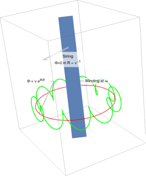
Figure 3: Cartoon of a cosmic string solution with the winding of the Higgs phase plotted on a transverse circle.

With the scalar potential $V(\Phi)$ minimized for some $|\Phi|=v\neq 0$, finite energy requires toward infinity in the transverse directions

$$\Phi(r,\theta)\rightarrow ve^{i\phi(\theta)}$$ (20)

where we may view $e^{i\phi(\theta)}$ as a map from the $S^{1}$ at transverse infinity to the $S^{1}$ of the gauge group. Such maps can be topologically classified by their winding number $k\in\mathbb{Z}$, the canonical example of which is $e^{ik\theta}$. Since $\Phi$ has charge $N$, the transformation $\phi\mapsto\phi+N\theta$ is a gauge symmetry and winding is only physical mod $N$.

The equations of motion for the gauge field then dictate setting at long distances

$$\vec{A}(r,\theta)\rightarrow\frac{\phi^{\prime}(\theta)}{eNr}\hat{\theta}.$$ (21)

With this we may directly relate the magnetic flux in the string to the winding number of the scalar using Stokes’ theorem. Starting with the definition of the winding number, we have

$$k=\frac{eN}{2\pi}\oint_{\gamma}\vec{A}\cdot d\vec{x} =\frac{eN}{2\pi}\int\int_{S}\vec{\nabla}\times\vec{A}\cdot d\vec{S}=\frac{eN}{2\pi}\Phi_{B}$$ (22)

$$\Rightarrow\Phi_{B}=\frac{2\pi}{eN}k,$$ (23)

where we have simply used Stokes’ theorem to relate the winding number to the magnetic flux $\Phi_{B}$ through the string. We see the flux carried by the string is fractionally quantized in $1/N$ of the Dirac flux quantum, $g_{D}=2\pi/e$ Dirac:1931kp ; Dirac:1948um . The strings then contain only a fraction of the flux around a Gaussian sphere of a fundamental magnetic monopole.

With nonzero winding number of the scalar field, these are then cosmic string solutions. The continuity of the field demands that somewhere in the interior $\Phi=0$ and the symmetry is unbroken. While the ultraviolet form of the solutions may be found in a given theory without much difficulty, we will here only need what could be guessed by dimensional analysis: there is a core of size $\sim v^{-1}$ inside which the Higgs is pushed up to the origin and the $U(1)$ is unbroken, and the strings have tension $E/L\equiv\mu\sim v^{2}$.

B.4 Discrete Aharonov-Bohm Effect

The cosmic string solutions we’ve described are cylindrical configurations with magnetic flux confined within a radius $R\sim v^{-1}$. This is a nearly-idealized solenoid, and indeed our long-distance solution for the vector potential in Eqn 21 is precisely that of the elementary Aharonov-Bohm setup Aharonov:1959fk . As they did, we consider shooting a charged fermion from point $p$ with initial wavefunction $\psi_{p}$ past a solenoid to an interferometer at point $r$, and we can write the resulting wavefunction as an integral over paths $\gamma$ from $p$ to $r$

$$\psi_{r}=\int_{p}^{r}\mathcal{D}\gamma e^{iS(\gamma)}\psi_{p}$$ (24)

where $S(\gamma)$ is the action evaluated for the path $\gamma$. We diagram this in Figure 4. The charged fermion has an electric current which in the nonrelativistic limit leads to an action contribution $\int d^{4}xA_{\mu}J^{\mu}\rightarrow q\int_{\gamma}A$. We assume no other terms are relevant. If the path integral has two saddle points $\gamma_{1},\gamma_{2}$, for example due to a screen with two slits between $p$ and $r$, then at lowest order $\psi_{r}$ is the superposition of these two paths

$$\psi_{r}\propto\left(e^{iq\int_{\gamma_{1}}A}+e^{iq\int_{\gamma_{2}}A}\right)\psi_{p},$$ (25)

and the probability density is then proportional to

$$\left|\psi_{r}\right|^{2} \propto\frac{1}{2}\left(2+e^{iq\int_{\gamma_{1}}A-iq\int_{\gamma_{2}}A}+e^{iq\int_{\gamma_{2}}A-iq\int_{\gamma_{1}}A}\right)\left|\psi_{p}\right|^{2}$$ (26)

$$\propto\left(1+\text{Re}\ e^{iq\oint_{\gamma}A}\right),$$ (27)

where $\gamma$ is the loop consisting of the path $\gamma_{1}$ composed with the path $\gamma_{2}^{-1}$. We see that the two paths interfere to the extent that $\exp iq\oint_{\gamma}A$ differs from one—that is, due to the presence of magnetic flux in the region encircled by $\gamma$.

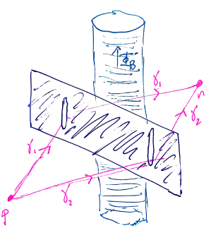
Figure 4: Cartoon of Aharonov-Bohm effect setup with two slits on either side of a solenoid providing inequivalent paths for electrons toward an interferometer.

In other language, the existence of the magnetic flux has induced a holonomy in the gauge field $A$, $\text{Hol}_{\gamma}(A)\equiv\exp i\oint_{\gamma}A\neq 0$. This is precisely the observable of the Aharonov-Bohm effect. A particle of electric charge $e$ transported around the solenoid then picks up a phase $\exp i\left(e\Phi_{B}\right)$. In the case of electromagnetism this is not quantized, since the magnetic flux through an experimentalist’s solenoid is ultimately proportional to the velocity of the electrons in the wires, which is a continuous parameter. But when electromagnetism is broken, as in a superconductor, or as above from an elementary Higgs field, magnetic flux is quantized into vortices. The AB effect for the Abelian Higgs with unbroken $\mathbb{Z}_{N}$ symmetry results in a phase from Eqn 23 of

$$\exp{ie\oint_{\gamma}A}=\exp{ie\frac{2\pi}{Ne}}=\exp\frac{2\pi ik}{N},$$ (28)

and we see that for a fundamental $N=1$ Higgs the Aharonov-Bohm effect vanishes in the broken phase. The $U(1)$ charge is completely screened and the vortices have magnetic flux $\Phi_{0}\equiv 2\pi/e$, which we recognize also as the flux through a sphere around a monopole with the Dirac charge quantum.

However, when the $U(1)$ symmetry is broken by a Higgs of charge $N>1$—such that the discrete $\mathbb{Z}_{N}$ gauge symmetry remains unbroken—the magnetic flux tubes are fractionally quantized with fundamental unit $\Phi_{B}=\Phi_{0}/N$. Then the Higgs condensate can only screen electric field lines in $N$-fold units, such that the charge $(\text{mod }N)$ is unscreened and a long-range $\mathbb{Z}_{N}$ gauge field remains Krauss:1988zc ; Alford:1989ch ; Preskill:1990bm ; Coleman:1991ku ; Banks:2010zn . A discretized version of the Aharonov-Bohm effect must therefore persist in the infrared. And indeed, we have seen that the winding of the Higgs field provides for dynamical solitons with discrete magnetic flux—precisely a fundamental particle version of the idealized solenoid.

Importantly this remaining discrete gauge symmetry implies their infrared stability even in the presence of magnetic monopoles. If we consider chopping off the top half of our solenoid to have a semi-infinite solenoid running off along the negative $z$ axis, at the origin we have a source of $\Phi_{B}$ magnetic flux. If $\Phi_{B}=\Phi_{0}$, then in the limit when the radius vanishes $R\rightarrow 0$, the solenoid becomes the unphysical Dirac string of Dirac’s $U(1)$ monopole. Then along a cosmic string one may imagine nucleating a monopole-anti-monopole pair which are pulled apart by the cosmic string tension and eat it up, as in Figure 5. But these monopoles simply cannot remove any fractional flux $\Phi_{B}/\Phi_{0}=k/N\ (\text{mod }1)$.

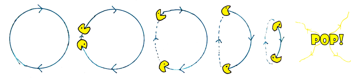
Figure 5: The so-called ‘pac-man’ instability of the minimal Abelian Higgs cosmic string loop to the nucleation of a monopole-antimonopole pair. With inspiration from R. Lichtenstein.

While the above experiment with solely two paths for the charged particle is a conceptually simple demonstration of the Aharonov-Bohm effect, the cosmologically relevant problem is simply of an incident charged particle on the solenoid. Building off earlier studies of AB scattering Aharonov:1984zza ; Rohm:1985aa ; deSousaGerbert:1988kpn ; deSousaGerbert:1988qzd ; Alford:1988sj ; Wilczek:1981du , including the original result of Aharonov and Bohm for a general solenoid Aharonov:1959fk , Alford & Wilczek looked at an example of cosmic strings from the breaking $SO(10)\rightarrow SU(5)\times\mathbb{Z}_{2}$ Alford:1988sj . The generalization of their result is a differential cross-section per unit length of

$$\frac{d\sigma}{d\theta}=\frac{\sin^{2}(\pi q\Phi_{B}/\Phi_{0})}{2\pi p\sin^{2}(\theta/2)},$$ (29)

with $p$ the incoming particle momentum, $q$ its charge, and $\Phi_{B}/\Phi_{0}$ the magnetic flux in fundamental units. There is then a large cross-section for elastic scattering due to the nontrivial gauge potential. The fundamental cosmic string has $\Phi_{B}/\Phi_{0}=1/N$, so that the Aharonov-Bohm scattering affects any particle with $q\neq 0\ (\text{mod }N)$.

The maximum is reached for $q=N/2$, the largest possible charge in $\mathbb{Z}_{N}$, but in our model with $N=2N_{c}{N_{g}}$ the suppression of elastic scattering from the $\sin^{2}$ is minor. For quarks with $q=1$, we have $\sin^{2}(\pi/18)\sim 3\times 10^{-2}$, and proton or lepton scattering is only suppressed by $\sin^{2}(\pi/6)=1/4$. Indeed, the cosmic strings have a large elastic scattering cross-section with all of the SM fermions. Such scattering affects neither the identity or energy of the scattered particles, but will lead to a drag force on cosmic strings moving in a dense medium.

B.5 $\mathbb{Z}_{N}$ Gauge Theory

In the far infrared of the $N$-Abelian Higgs when only the discrete $\mathbb{Z}_{N}$ gauge theory remains, the physics can be made more transparent by dualizing $\phi$ to a two-form gauge field $B_{\mu\nu}$, as first done in Banks:1989ag ; Coleman:1991ku and later emphasized in Banks:2010zn . Beginning with the infrared Lagrangian of Equation 19, we first rewrite it as

$$\mathcal{L}=-iJ^{\mu}(\partial_{\mu}\phi-eNA_{\mu})-\frac{1}{2v^{2}}J^{\mu}J_{\mu},$$ (30)

which can be seen to produce the same Lagrangian upon setting $J^{\mu}$ to its equations of motion $J_{\mu}=-iv^{2}(\partial_{\mu}\phi-eNA_{\mu})$. If we instead integrate the first term by parts, then we can interpret $\phi$ as merely a Lagrange multiplier enforcing the constraint $\partial_{\mu}J^{\mu}=0$.

We can trivialize this constraint on the dual current by changing variables as

$$J_{\mu}=-\frac{i}{2\pi}\epsilon_{\mu\nu\rho\sigma}\partial^{\nu}B^{\rho\sigma}$$ (31)

where $\epsilon_{\mu\nu\rho\sigma}$ is the Levi-Civita symbol and $B$ is an antisymmetric two-tensor field. The two-tensor $B_{\mu\nu}$ is invariant under a gauge transformation by an exact two-form $B_{\mu\nu}\rightarrow B_{\mu\nu}+\partial_{\left[\mu\right.}\lambda^{(1)}_{\left.\nu\right]}$ parametrized by a one-form $\lambda^{(1)}$ in a higher-dimensional analogue of the one-form gauge symmetry of electromagnetism $A_{\mu}\rightarrow A_{\mu}+\partial_{\mu}\lambda^{(0)}$.

When we then rewrite the Lagrangian in terms of this two-form and look at low energies we find

$$\mathcal{L} =\frac{eN}{2\pi}A^{\mu}\partial^{\nu}B^{\rho\sigma}\epsilon_{\mu\nu\rho\sigma}$$ (32)

$$=-\frac{N}{2\pi}B\wedge F,$$

the so-called ‘BF theory’ first introduced by Horowitz Horowitz:1989ng ; Blau:1989bq ; Blau:1989dh ; Wu:1990ci , where in the second line we’ve cleaned up the indices by instead writing a wedge product of two-forms (and also put the coupling back into $A$). In the IR the kinetic terms for the $A,B$ fields disappear, meaning that there are no local degrees of freedom, as expected.

Nonetheless, the theory is not entirely trivial: The BF theory is a topological theory of an Abelian one-form gauge field $A$ and an Abelian two-form gauge field $B$. With just our two gauge fields, we have as observables the Wilson lines $\exp in_{A}\int_{\Sigma_{1}}A$ and Wilson surfaces $\exp in_{B}\int_{\Sigma_{2}}B$, where $\Sigma_{d}$ is a $d$-dimensional surface and $n_{A},n_{B}$ are integers. These capture the effects of the gauge field on the phase of the wavefunction for a probe particle which has no other dynamics. As effective field theorists, we may think of these as the infrared remnants of massive charge-$n_{A}$ particles with worldline $\Sigma_{1}$ or massive strings of winding $n_{B}$ with worldsheet $\Sigma_{2}$. Indeed, the one-dimensional objects charged under the two-form gauge symmetry are none other than the cosmic strings we studied above. Our absorption of the charge $e$ into the gauge field $A$ puts the Wilson operators on equal footing in terms of solely the integers $n_{A},n_{B}$ appearing. Alternatively we could have rescaled $B$ to make explicit its coupling, which is $v^{-1}$.

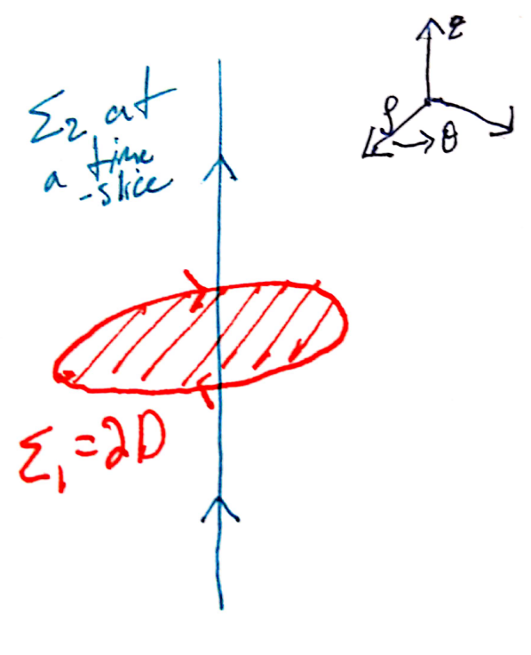
Figure 6: Example configuration for a two-observable correlator in the BF theory with $\Sigma_{1}$ spacelike and $\Sigma_{2}$ at $x=y=0$.

Furthermore, the topological interaction gives precisely the appropriate Aharonov-Bohm phases as these wind around each other, and ensures that only $n_{A}n_{B}\ (\text{mod }N)$ is observable. This is the signature of the $\mathbb{Z}_{N}$ gauge symmetry at low energies. One can calculate the expectation value of a Wilson loop and a Wilson surface to find

$$\left\langle e^{in_{A}\int_{\Sigma_{1}}A}\ e^{in_{B}\int_{\Sigma_{2}}B}\right\rangle=\exp{\left[2\pi i\frac{n_{A}n_{B}}{N}\text{link}(\Sigma_{1},\Sigma_{2})\right]},$$ (33)

where $\text{link}(\Sigma_{1},\Sigma_{2})$ is the linking number of these two manifolds and in some sense this can be used to define generalized linking numbers quantum field theoretically Oda:1989tq ; Horowitz:1989km . This can be understood by recognizing that BF theories are naturally theories of de Rham cohomology groups of fiber bundles, but we can convince ourselves of this in a more elementary fashion with inspiration from our above discussion of the AB effect.

Our strategy is to push the Wilson surface operator into the action, and reinterpret this as the expectation value of the Wilson loop in a background of a probe string. We let $X^{a}$ be coordinates on $\Sigma_{2}$, and $x^{\mu}=\xi^{\mu}(X^{a})$ the position of the surface in spacetime, and set $n_{A}=n_{B}=1$ for cleanliness. We have

$$\left\langle e^{i\int_{\Sigma_{1}}A}e^{i\int_{\Sigma_{2}}B}\right\rangle=\int\mathcal{D}A\mathcal{D}Be^{i\int_{\Sigma_{1}}A}e^{i\left(S_{BF}+\int_{\Sigma_{2}}B\right)},$$ (34)

where the action has been modified to

$$S_{BF+B}=\int d^{d}x\ \left(-\epsilon_{\mu\nu\rho\sigma}\frac{N}{2\pi}\partial^{\mu}A^{\nu}B^{\rho\sigma}+B_{\mu\nu}\delta^{(2)}\left(x-\xi(X)\right)\frac{\partial\xi^{\mu}}{\partial X^{a}}\frac{\partial\xi^{\nu}}{\partial X^{b}}\epsilon^{ab},\right)$$ (35)

and we can reinterpret this as adding to our Lagrangian an operator to create an extended object, which the delta function localizes to a submanifold Brennan:2021a . We can make the simple gauge choice $\xi^{\mu}(X)=\delta^{\mu}_{a}X^{a}$ to make the Jacobian trivial. Now by examining the equation of motion from varying $B$, we see that this term induces a fractional flux for the gauge field $A$,

$$\frac{\delta\mathcal{L}}{\delta B^{\sigma\rho}}=-\epsilon_{\mu\nu\rho\sigma}\frac{N}{2\pi}\partial^{\mu}A^{\nu}+\delta^{(2)}\left(x-X\right)\delta_{\rho}^{a}\delta_{\sigma}^{b}\epsilon_{ab}=0.$$ (36)

To make the physical picture clearer, let’s specialize to the case of $\Sigma_{2}$ the worldsheet of a static cosmic string at $X^{a}=(t,z)$, and $\Sigma_{1}$ a spatial loop which encircles the $z$-axis, as in the Aharonov-Bohm setup. Then the equation of motion for $\rho=t,\sigma=z$ gives us

$$\vec{\nabla}\times\vec{A}=\frac{2\pi}{N}\delta\left(x\right)\delta\left(y\right)\hat{z},$$ (37)

and this is nothing other than an induced fractional holonomy for the gauge field around the string. If we integrate this over a spatial surface $D$ with $\partial D=\Sigma_{1}$, then it is clear that if $\Sigma_{1}$ loops around the spatial $S_{1}$ of $\Sigma_{2}$ we have

$$\oint_{\Sigma_{1}}A=\int_{D}\nabla\times A=\frac{2\pi}{N}.$$ (38)

Then we can use this modified equation of motion for $A$ in evaluating the expectation value and find

$$\left\langle e^{i\int_{\Sigma_{1}}A}\right\rangle_{BF+B}=e^{2\pi i/N},$$ (39)

precisely the holonomy we saw in Appendix B.4 appearing for a unit-charged particle transported around a fundamental cosmic string in the non-minimal Abelian Higgs. The general result of Equation 33 should then be thought of as the relativistic generalization of the discrete Aharonov-Bohm effect to arbitrary line and surface operators.

Indeed, the cosmic strings of the Abelian Higgs theory source the two-form gauge field $B_{\mu\nu}$, and the Wilson surfaces are their remnant in the IR $\mathbb{Z}_{N}$ gauge theory as non-dynamical sources. Just as in the Abelian Higgs description, the strings induce a holonomy $e^{2\pi i\Phi_{B}/\Phi_{0}}\in\mathbb{Z}_{N}$ for the gauge field $A$. We will return to the BF theory in Appendix D, but its full application to our scenario will be further studied elsewhere. In the meantime, reviews of discrete gauge theories include deWildPropitius:1995hk ; Alford:1991vr ; Birmingham:1991ty .

Appendix C Cosmic String Dynamics

In this section we review some qualitative features of the formation and evolution of cosmic strings. Ultimately our interest will be in an early-time and small-scale regime where the details and not yet known, so we will resort simply to parametrizing the string number density, as above. But understanding the features below is still a useful guide to their behavior.

C.1 Cosmic String Evolution

In the cosmological case of a dynamical phase transition in the early universe, the production of cosmic strings is guaranteed by the finite size of the cosmic horizon. The field $\Phi$ condenses with independent phases in different Hubble patches, so line defects necessarily form. The string formation may be thought of as a random walk, which in three spatial dimensions need not return to its starting point. So an order one number of super-Hubble length cosmic strings per Hubble volume is expected to form by simple dimensional analysis. This was first studied by Kibble Kibble:1976sj ; Kibble:1980mv and the formation of such topological defect solutions is sometimes known as the ‘Kibble mechanism’. Numerical simulations thereafter Vachaspati:1984dz confirmed that an order-one fraction of the energy density in strings during formation is in infinite, horizon-crossing strings.

Resultingly, the exotic solutions to the Abelian Higgs equations of motion that we constructed in Sec B.3 are not merely of formal interest, but are necessarily realized in the early universe. In the following section we will discuss the evolution of these objects after the phase transition in which they are formed. The strings are not charged under any unbroken continuous gauge symmetries, so there are no massless gauge bosons mediating long-range forces. As a result, the long-range dynamics of an isolated string are purely gravitational and controlled by the classical Nambu-Goto action of a gravitating string Nambu:1970a ; Goto:1971ce ; Forster:1974ga .

We note that there is lots of physics in the details of the Kibble mechanism and the spectrum of defects formed, and this connects closely to condensed matter realizations thereof. In particular, the correlation length of Higgs fluctuations may in fact be quite small compared to the horizon length $\xi\ll d_{h}$, resulting in a far greater initial number density of defects Guth:1982pn ; Zurek:1985qw ; Murayama:2009nj . Our scenario will need to rely on this early-time overabundance of strings, but this is not yet well-understood.

The late-time behavior is still non-trivial and quite interesting. There is an infamous result that cosmic strings reach an attractor solution where the string network has a scaling symmetry—the distribution of string loop lengths depends solely on the length as a fraction of the Hubble radius. This was first argued for on energetic grounds by Turok and collaborators Albrecht:1984xv ; Turok:1984db , with the only other possibility being overclosing the universe Kibble:1984hp . Simulations by Bennett & Bouchet provided numerical evidence for the scaling regime near the horizon scale shortly thereafter Bennett:1987vf ; Bennett:1989ak ; Bennett:1989yp ; Sakellariadou:1990nd ; Allen:1990tv . Analytic arguments for the scaling solution were later given by Kibble & Copeland Martins:1996jp ; Kibble:1990ym ; Copeland:1991kz ; Austin:1993rg , but confusion reigned about the situation on small scales, with some simulations finding copious production of small loops Vincent:1996rb and uncertainty about the role of ‘kinks’ and other structure on the strings Kibble:1990ym ; Siemens:2001dx ; Siemens:2002dj . Increasingly powerful simulations have further confirmed the scaling regime Moore:2001px ; Ringeval:2005kr ; Martins:2005es ; Vanchurin:2005pa ; Olum:2006ix ; Blanco-Pillado:2011egf ; Blanco-Pillado:2013qja ; Hindmarsh:2008dw ; Auclair:2019zoz . A microphysical explanation in terms of the classical string theory was finally provided by Polchinski & Rocha Polchinski:2006ee ; Polchinski:2007rg ; Rocha:2007ni ; Dubath:2007mf ; Lorenz:2010sm , with Polchinski:2007qc giving a nice overview of the difficulties of this problem.

What this means is that the late-time behavior is controlled by strings chopping each other up into loops and ensmallening by emitting gravitational radiation. We will discuss these effects in the next two sections.

However, before the late-time attractor dynamics can take over, there is a period when friction from elastic Aharonov-Bohm interactions with the SM plasma dominates. That cosmic strings dominantly interact with matter through the Aharonov-Bohm effect was first appreciated only in 1989 by Alford & Wilczek Alford:1988sj . As we saw in Sec B.4, the string elastically scatters charges at an enormous rate $\sigma/\ell\sim 1/p$, with $p$ the momentum. This scattering from the gauge potential is far more important than the friction due to gravitational effects which had previously been considered Everett:1981nj ; Vilenkin:1984ib ; Silva:2021www .

Vilenkin then showed Vilenkin:1991zk that in the rest frame of a straight section of string moving at $\vec{v}$ with respect to the background gas of particles with charge $q$ at temperature $T$, the frictional force is

$$\vec{F}\simeq-T^{3}\frac{\vec{v}}{\sqrt{1-v^{2}}}\sin^{2}(\pi\frac{qk}{N}).$$ (40)

where I’ve gotten rid of some numerical factors. The effect on the string is to damp out motion on a timescale $\propto\mu/T^{3}$. This frictional force turns out to severely damp the dynamics until $T\lesssim(G\mu)M_{\text{pl}}$, when the strings can begin free-streaming. See also Garriga:1993gj ; Martins:1995tg .

While a single, long, straight string is easy enough, an understanding of the dynamics when they free-stream quickly becomes very complicated. There are an enormous range of scales involved in the problem—from the Hubble scale, to the interstring distance, to the curvature length along the string, down to the fundamental transverse size of the string. For fundamental cosmic strings, the interactions are controlled by a string coupling which may be small. However, our strings are semi-classical and have no free limit. As a result, the strings strongly self-interact. The Polyakov dynamics Polyakov:1981rd break down entirely when strings intersect each other, or themselves, and the results of these interactions are crucial for understanding the network dynamics.

For completeness, I briefly note here the interesting program of understanding the cosmic string behavior using the worldsheet theory derived from the Abelian Higgs theory (e.g. Gregory:1988qv ; Akhmedov:1995mw ; Gregory:1990pm ; Silveira:1993am ; Orland:1994qt ; Arodz:1995dg ; Baker:1999xn ; Baker:2000ci ; Aharony:2013ipa ; Szabo:1998ej ; Bergeron:1994ym ; Zee:1994qw ; Sato:1994vz ).

C.2 Intercommutation

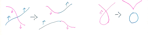
Figure 7: Cartoon of intercommutation dynamics whereby colliding string exchange partners,and self-intersecting strings chop off loops.

There is a counter-intuitive effect in string scattering which turns out to be crucial to our phenomenology: colliding Abelian Higgs cosmic strings always ‘intercommute’ (or ‘reconnect’ or ‘trade ends’ or ‘exchange partners’), as diagrammed in Figure 7. This effect has been seen numerically to apply quite broadly, but as far as I am aware there is analytic understanding only in the case of supersymmetric defects, so we discuss that case to gain some qualitative conceptual insight.

That understanding begins with Ruback Ruback:1988ba , who found in $2+1$d that identical vortices undergo right-angle scattering by following the moduli space approximation introduced by Manton Manton:1981mp for monopoles and eventually rigorously justified by Stuart Stuart:1994tc ; Stuart:1994yc , see also Atiyah:1985dv ; Gibbons:1986df ; Rosenzweig:1990ea ; Samols:1991ne ; Abdelwahid:1993fg ; MacKenzie:1995np ; Gauntlett:2000ks . Topological defects at low energy follow geodesics on the moduli space, with a metric derived from the kinetic terms in the Lagrangian.

In the case of two identical vortices colliding at low energies, the only relevant coordinate on the two-vortex moduli space is the relative position $\vec{r}$ pointing from the zero in the Higgs field of one to the other. So the moduli space in the winding number $k=2$ sector looks locally like the plane $\mathbb{R}^{2}$. But despite being semi-classical objects, two vortices may be identical and so indistinguishable, so $-\vec{r}$ describes the same configuration. Then the moduli space has the geometry of a cone with deficit angle $\pi$—at least at large separations. But it’s more difficult to reason about the behavior near the tip, since at small distances $|r|\lesssim v^{-1}$ the vortices lose their separate identities and our above argument fails.

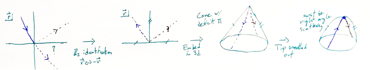
Figure 8: Cartoon of motion in the two-vortex moduli space. Since the vortices are indistinguishable, the space is a cone, though the tip is smoothed out. The radial geodesic then clearly passes straight over the cone, which in physical space corresponds to right-angle scattering.

In fact the moduli space is known to be smooth Taubes:1979tm so that the cone must be rounded off, and indeed in solvable UV-completions one can explicitly see the tip of the cone smoothed out Hanany:2005bc ; Hashimoto:2005hi . Then the intuitive picture is clearer, and we’ve diagrammed the situation in Figure 8. An ingoing radial geodesic goes straight over the cone, and this corresponds in physical space to a scattering angle of $\pi/2$, whereas forward scattering would correspond to a geodesic ‘bouncing back’ at the same angle after hitting $\rho=0$. We try to diagram this logic in Figure 8.

The $2+1$d right-angle scattering can be uplifted to cosmic string intercommutation by projecting the motion of the $3+1$d strings down to the motion of the cores in various planes Shellard:1988ki ; Hashimoto:2005hi ; Tong:2005un , as in Figure 9. The fluxes pass through some such planes in the same direction, in which case the motion on the plane is of vortices undergoing right-angle scattering, but the fluxes pass oppositely through other planes on which the interaction is of vortex-antivortex annihilations. Intercommutation necessarily follows from the consistency of these lower-dimensional interactions.

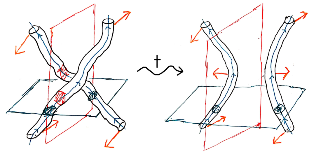
Figure 9: Cartoon of an interaction between cosmic strings, zoomed in near the collision point. Orange arrows give the string velocities, which are initially into/out of the page. The configuration can be projected onto the red plane through which the string fluxes pass in different directions, such that the motion of the zeros of the Higgs field on this plane looks like vortex-antivortex annihilation. On the other hand, projecting onto the green plane the motion is of right-angle vortex-vortex scattering. Consistency with these 2+1d dynamics implies that after the collision the strings have exchanged ends—they must intercommute. Heavily inspired by Figure 1 of Hashimoto:2005hi .

Numerical simulations of the underlying field theory dynamics have also been used to investigate the string dynamics during collisions Shellard:1987bv ; Shellard:1988zx ; Matzner:1988qqj ; Moriarty:1988em ; Myers:1991yh , and indeed are in agreement with the intercommutation probability being near unity. The string network simulations we will match to use the Nambu-Goto action to evolve their numerical strings and then merely implement intercommutation by hand whenever a collision is detected. Given the enormous range of scales in the problem it seems untenable to resolve the microphysical interaction, though we note recent work on axion strings using adaptive mesh refinement methods which may help also in this case Buschmann:2021sdq .

This intercommutation is crucial to prevent the string network from dominating the energy budget of the universe Albrecht:1984xv ; Turok:1984db . Such interactions chop strings into smaller pieces, and lead to a distribution of lengths of string loops being created at any time, as we will see in Sec C.4. The many loops chopped off in such processes allow the network to dissipate energy by emitting gravitational radiation as they oscillate.

We note also that each intercommutation leads to the formation of ‘kinks’—small-scale structure originating at the interaction point and then travelling in left- and right-moving modes (see e.g. Blanco-Pillado:2015ana ; Kibble:1990ym ; Copeland:2009dk ; Kibble:1990ym ; Siemens:2001dx ; Siemens:2002dj ; Rosenzweig:1990ea ). We defer further understanding of the effects of this small-scale structure to future work—if anything, it seems sensible to expect this to result in a larger number of small loops produced by the network (e.g. Dubath:2007mf ), so that ignoring this is in some sense conservative.

C.3 Diminution

Energy loss by string loop radiation is then an important effect for understanding the network dynamics Vilenkin:1981bx ; Vilenkin:1981kz . In the string rest frame the power emitted into gravitational waves from a string loop of length $\ell$ oscillating at a frequency $\omega$ is given by the ‘quadrupole formula’ and estimated as Vilenkin:2000jqa

$$\frac{dM}{dt}\sim G\left(\frac{d^{3}Q}{dt^{3}}\right)^{2}\sim GM^{2}\ell^{4}\omega^{6}\sim G\mu^{2}$$ (41)

where $Q\sim M\ell^{2}$ is the approximate quadrupole moment of the string loop and $\omega\sim\ell^{-1}$ is the characteristic frequency. This results in an energy loss which is independent of the overall size of the string, and simulations have found $\dot{M}=\Gamma G\mu^{2}$ with $\Gamma$ a numerical coefficient of order $\Gamma\sim 50$. We note also that strings may well radiate more than just gravitons Vilenkin:1986zz ; Cui:2008bd ; Long:2014lxa ; Long:2014mxa ; Hindmarsh:2017qff ; Long:2019lwl ; Auclair:2019jip ; Vachaspati:2009jx ; Hyde:2013fia ; Lunardini:2012ct ; Vachaspati:2009kq ; Damour:2001bk , and this fact may be used for interesting phenomenological ends (see e.g. Bhattacharjee:1982zj ; Brandenberger:1991dr ; Brandenberger:1992ys ; Davis:1992fm ; Ma:1992ky ; Lew:1993bb ; Brandenberger:1994mq ; Mohazzab:1994xj ; Sato:1995ea ; Davis:1996zg ; Sahu:2004ir ; Sahu:2005vu ).

On large distances the cosmic strings are expected to behave as Nambu-Goto strings, and to have universal gravitational effects which offer the best observational prospects for general cosmic strings. The gravitational effects are dominated by the long strings, which carry an order one fraction of the energy density, so our understanding of this limit has seen intense study. But our interest is in the total number density, which will be dominated by small loops. And so the behavior which has yet been understood precisely does not suffice for our interests, malheureusement. As to smaller scales, Eqn 41 motivates the definition of a dimensionless ‘gravitational cutoff’ or ‘gravitational backreaction scale’ $\xi\sim G\mu$, such that at time $t$, a loop of length $\ell\sim G\mu t$ would disappear entirely in a Hubble time. The behavior of such small loops remains the subject or debate.

The evolution at the smallest scales further depends on the stability properties of the strings. While in the low-energy theory the cosmic strings are topologically stable as a result of the remnant $\mathbb{Z}_{N}$ symmetry discussed above, this stability is challenged when the radial mode can jump over the barrier at the origin of field space or tunnel through it. Thus once a string loop has shrunk in size to near the symmetry-breaking scale $\ell\sim v^{-1}$, the remnant discrete gauge symmetry does not prevent it from further shrinking to nonexistence.

However, these loops may be stabilized by the presence of superconducting currents Witten:1984eb ; Davis:1988ip ; Davis:1988jq if there are appropriate degrees of freedom living on their cores. These ‘vortons’ are then stabilized against further decay after reaching a small size where the repulsive effect of angular momentum prevents further dissipation Carter:1990sm . Interestingly, the stability properties may be affected by degrees of freedom which are heavy in vacuum, but have massless excitations on the string worldsheet. Indeed, depending on the UV field content some relic vortons are inevitable Auclair:2020wse , which places an upper limit on the string tension $G\mu$ so the vortons do not overclose the universe Peter:2013jj . In the case $G\mu\lesssim 10^{-15}$, stable vortons may comprise some part of the dark matter density.

Our benchmark scenario is of strings which are ultimately unstable, but below we will also calculate the number density for the case in which strings are stable. Of course a realistic model may lie somewhere between these, with a fraction of strings ending up as vortons and others decaying.

C.4 Scaling from Simulations

As we discussed in Appendix C.1, we know now with confidence that the cosmic string network has a scaling solution at distances near the horizon length. The interplay of long strings entering the horizon, intersections of strings chopping off loops, and gravitational radiation emission leads to an attractor solution with self-similar dynamics. As this is the only regime in which the evolution is under control, we will make the simplifying assumption that we enter it instantaneously at some time $t_{\star}$ when the scale factor is $a_{\star}$.

But it is important to note that many uncertainties remain. We will assume the scaling regime extends down to the gravitational backreaction scale, which is further than numerical simulations have been able to test. We note also that some simulations have found a lengthy ‘transient’ regime before scaling is reached, so it is possible that $t_{\star}$ may be long after the phase transition. During this approach to scaling, it has been found that small loops are overproduced (e.g. Olum:2006ix ), but as far as I am aware this transient regime has not been well-characterized.

We will follow the formalism of Blanco-Pillado:2013qja and describe the distribution of strings using the scaling length variable $\alpha\equiv m/(d_{h}\mu)$ with $m$ the mass of the string and $\mu$ the string tension. The scaling regime implies that the loop production as a function of cosmic time and loop mass depends only on the ratio $\alpha\propto m/t$. In the following section we will sum up the total number density of loops in the scaling regime.

The behavior can be qualitatively understood quite simply: In scaling, the network produces a constant number of loops per Hubble spacetime volume. In a cosmology with equation of state $w>-1/3$ (e.g. radiation or matter domination), the Hubble size grows more quickly than does the physical volume. Then the same loop production is spread over a larger physical volume at later times, so it is the early production of loops that matters most.

We use the formalism and numerical results of Blanco-Pillado:2013qja as a benchmark. We define a momentum-integrated form on the string loop phase space as $f(t,m)=\int f(t,m,p)\text{d}p$, and then $f(t,m)\Delta t\Delta m$ gives a comoving number density of loops produced in time $t\dots t+\Delta t$ with mass between $m\dots m+\Delta m$. We wish to sum up the production of loops over time using the production function found numerically.

The results of simulations in the scaling regime are characterized in terms of a scaling production function $f(\alpha)\Delta\alpha$. At a fixed time $t$, this may be interpreted as the number of loops produced in a Hubble volume $d^{3}_{h}$ over a Hubble time $d_{h}$ with mass $m=d_{h}\mu\alpha\dots d_{h}\mu(\alpha+\Delta\alpha)$. We can then relate the two functions as

$$\frac{f(\alpha)\Delta\alpha}{d^{4}_{h}}=\frac{f(t,m=d_{h}\mu\alpha)\Delta m}{a^{3}}$$ (42)

and in the limit $\Delta m/\Delta\alpha\rightarrow\left.\frac{\partial m}{\partial\alpha}\right|_{t}=d_{h}\mu$ we have

$$\left.f(\alpha)\right|_{t}=\frac{\mu d^{5}_{h}}{a^{3}}f(t,m=d_{h}\mu\alpha).$$ (43)

Simulations have found power-law scaling behavior of the sort

$$f(\alpha)\text{d}\alpha\sim\frac{\text{d}\alpha}{\alpha^{p}}$$ (44)

with $p>1$, so the production is peaked toward small loops. Though simulations are limited by their resolution to explore only a few decades below the Hubble scale, we will extrapolate this production down to the gravitational backreaction scale $\xi\sim G\mu$, taking $m_{\text{min}}(t,t)=\xi\mu d_{h}$.

The coefficient is by definition independent of $\alpha$, which is the only relevant parameter by the scaling symmetry, so a coefficient of order unity is indeed borne out by simulations. As for the exponent $p$, we will use $p=1.7$ as a benchmark, which is the value determined during the matter-dominated era by Blanco-Pillado:2013qja . As our purpose is just to evince the parametrics and show the number density of string loops may be large enough, we will not delve into the full body of work determining the precise form of scaling, work on which may be found in e.g. Allen:1990tv ; Bennett:1985qt ; Bennett:1986zn ; Bennett:1987vf ; Bennett:1989ak ; Bennett:1989yp ; Albrecht:1989mk ; Hindmarsh:2008dw ; Polchinski:2006ee ; Polchinski:2007rg ; Lorenz:2010sm ; Auclair:2019zoz ; Vanchurin:2005pa ; Ringeval:2005kr ; Martins:2005es ; Blanco-Pillado:2011egf ; Blanco-Pillado:2013qja ; Martins:1996jp ; Martins:1995tg ; Vincent:1996rb ; Copeland:1991kz ; Blanco-Pillado:2019tbi ; Rocha:2007ni ; Almeida:2021ihc .

Small Loop Enhancement

If we have a loop production function in terms of the comoving number density, then we can find the total number of loops simply by adding up the loops produced at each time. We must translate the constant production per Hubble spacetime volume to the comoving volume.

$$n(t) =\int^{t}_{t_{\star}}dt^{\prime}\int_{m_{\text{min}}(t^{\prime},t)}dm^{\prime}f(t^{\prime},m^{\prime})$$ (45)

$$=\int^{t}_{t_{\star}}dt^{\prime}\int_{\alpha_{\text{min}}(t^{\prime},t)}\frac{a^{\prime 3}}{d^{\prime 5}_{h}\mu}f(\alpha^{\prime})d\alpha^{\prime}d^{\prime}_{h}\mu$$ (46)

$$=\int^{t}_{t_{\star}}\frac{dt^{\prime}}{d^{\prime}_{h}}\frac{a^{\prime 3}}{d^{\prime 3}_{h}}\int_{\alpha_{\text{min}}(t^{\prime},t)}f(\alpha^{\prime})d\alpha^{\prime}$$ (47)

If loops are stable, we can simply sum over all loops produced at each time, taking $\alpha_{\text{min}}(t^{\prime},t)\equiv\xi$, the gravitational cutoff scale. But if loops are unstable, we must only sum over those which will not have disappeared by $t$. Then we should take

$$m_{\text{min}}(t^{\prime},t) =\xi\mu\left(d_{h}+t-t^{\prime}\right)$$ (48)

$$\alpha_{\text{min}}(t^{\prime},t) =m_{\text{min}}(t^{\prime},t)/(\mu d^{\prime}_{h})$$ (49)

for which a loop produced with scaling mass $\alpha_{\text{min}}$ at time $t^{\prime}$ has shrunk to the cutoff scale $\xi$ at time $t$. Then with a power-law loop production function we have

$$n(t)=\int^{t}_{t_{\star}}\frac{dt^{\prime}}{d^{\prime}_{h}}\frac{a^{\prime 3}}{d^{\prime 3}_{h}}\xi^{1-p}$$ (50)

in the stable case, and

$$n(t)=\int^{t}_{t_{\star}}\frac{dt^{\prime}}{d^{\prime}_{h}}\frac{a^{\prime 3}}{d^{\prime 3}_{h}}\xi^{1-p}\left[\frac{\left(d_{h}+t-t^{\prime}\right)}{d^{\prime}_{h}}\right]^{1-p}$$ (51)

when loops are ultimately unstable. When solely one sort of background evolution is relevant, we have $d^{\prime}_{h}=t^{\prime}/(1-\nu)$ and $a^{\prime}=a_{\star}(t/t_{\star})^{\nu}$. During radiation domination, $\nu=1/2$, and during matter domination, $\nu=2/3$.

In the stable case the integral may be done immediately, to find

$$n(t)\simeq\xi^{1-p}\frac{a_{\star}^{3}}{t_{\star}^{3}}$$ (52)

where we have left off some order-one factors involving $\nu$ for readability, and ignored a term which vanishes as $t_{\star}/t\rightarrow 0$. We see that indeed the early loop production matters most so that the physical loop number density just dilutes as $1/t^{3\nu}$, as for a gas of particles.

Since early loop production is most important, the number density in the unstable case may be computed easily noting that at early times $\frac{\left(d_{h}+t-t^{\prime}\right)}{d^{\prime}_{h}}\rightarrow\frac{2-\nu}{1-\nu}\frac{t}{t^{\prime}}$. One finds

$$n(t)\simeq\xi^{1-p}\frac{a_{\star}^{3}}{t_{\star}^{3}}\left(\frac{t_{\star}}{t}\right)^{p-1}$$ (53)

and we see that the suppression is by a factor $\left(\frac{t_{\star}}{t}\right)^{p-1}$ with respect to the stable case. Now the physical number density dilutes as $1/t^{3\nu+p-1}$.

As is clear from Equations 52 & 53, our estimate for the total string loop number density depends upon our assumptions about the behavior of the cosmic string network at early times $t_{\star}$ and at small scales $\xi$. But the conclusion we take from this to use in our benchmark is that there may be a quite large abundance of small cosmic string loops—for a symmetry-breaking scale of order a TeV, the enhancement in the number density of small cosmic strings from $\xi^{1-p}$ may be upwards of $10^{20}$.

Appendix D Topological Defect Catalysis

We will discuss the specific example of cosmic string catalysis borne out by our model in Sec D.3. However, the conceptual physical understanding of the catalysis effect is rather opaque in that case as yet. This is such an exotic effect—in the sense of being far from free field theory—that to build intuition and aid further understanding we begin with exploring similar, more-familiar effects for topological defects of lower dimensionality.

Topological defects are a rich topic in field theory going back all the way to Dirac, who first puzzled over the interactions of charged fermions with magnetic monopoles. It is from this setting that we adopt the term ‘catalysis’, which comes from the Callan-Rubakov effect of GUT monopoles catalyzing proton decay. In this example the need for inelastic interactions can be seen elementarily from the far infrared. There has been much progress in the last century of understanding both the infrared and ultraviolet pictures of the electric and magnetic charges.

While it is not usually referred to with this language, the nontrivial intertwining of charged fermions with instantons has also been appreciated since ’t Hooft. The physics of these zero-dimensional topological defects is naturally understood in fully Euclidean space, and this makes it easy to see the role and peculiarity of fermion zero modes and the violation of anomalous symmetries. The drawback and disambiguation with the other cases is that instantons do not have a relic abundance and do not truly undergo scattering, so an assertion of ‘unitarity-limited’ interactions is not immediately sensible. But we nonetheless distinguish between some large action cost for producing the instanton, and the fermion interactions which come along with unit probability.

Taking these together, we find it natural to conjecture that all of the phenomena discussed admit some sort of unified description—perhaps in the language of generalized global symmetries—but the analogy has thus far not been made precise. We will below try to call attention to the similarities, but a full exploration is postponed to future work.

At the very least, we can speak about the defects in the general case in topological language. In this section our scenario of interest is the classical, static Yang-Mills(-Higgs) equations of motion solved on a sphere at the compactification of asymptotic infinity of some number of spatial dimensions $S^{k}$. The configuration space in this problem for a gauge theory of the group $G$ (possibly spontaneously broken to the subgroup $H$) consists of the gauge boson $A$ (and scalar $\Phi$) fields, which are locally defined maps from this sphere at infinity into the gauge group $S^{k}\rightarrow G$ (or $S^{k}\rightarrow G/H$). Such maps are classified by the homotopy group $\pi_{k}(G)$ (or $\pi_{k}(G/H)\simeq\pi_{k-1}(H)$) which counts the topologically distinct sectors—a generalized notion of ‘winding numbers’. These classify the topological defects in a given theory.

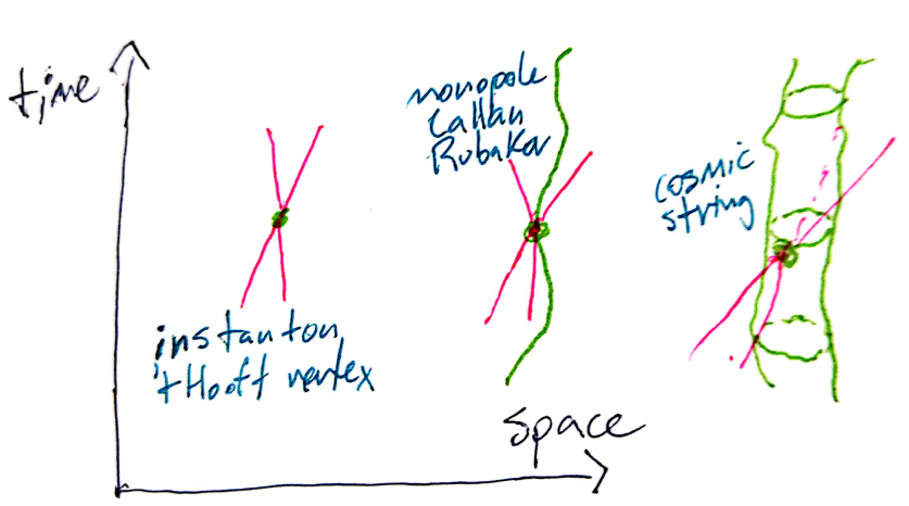
Figure 10: Cartoon of catalysis processes for topological defects of different dimensions.

D.1 Instantons and Fermi Zero-Modes

Instantons in Yang-Mills theories are dimension-zero topological defects. Such solutions exist when there are nontrivial maps from the boundary of Euclideanized spacetime to the gauge group. In the unbroken electroweak case, maps $W:S^{3}\rightarrow SU(2)\cong S^{3}$ are classified by a winding $\mathbb{Z}$. Instanton configurations are those with nonzero topological charge $\int W\tilde{W}/(16\pi^{2})\neq 0$, and the field non-trivially winds around spacetime.

D.1.1 Infrared Inelastic Interactions

The inclusion of fermion fields in the path integral can qualitatively affect the instanton solutions through the presence of fermionic zero-modes. ‘Zero-modes’ refers to zero-energy eigenmodes of the Hamiltonian, and in the bosonic case these are the ‘collective coordinates’ of the object—be they orientation in the physical space or in an internal space as a result of Higgsing. However, Pauli-Fermi-Dirac exclusion leads fermionic zero-modes to behave quite differently. With a given background of the (Euclidean) metric and gauge fields, we follow Fujikawa Fujikawa:1979ay and diagonalize the fermions’ quadratic action using the Dirac eigenspinors $\varphi_{n}(x)$

$$\gamma^{\mu}D_{\mu}\varphi_{n}=\lambda_{n}\varphi_{n}$$ (54)

where $\gamma^{\mu}D_{\mu}\equiv\not{D}$ is the Hermitian Dirac operator for that background and $\lambda_{n}$ are the real eigenvalues. We can write Grassmann-valued Dirac fields $\psi,\bar{\psi}$ in terms of Grassmann coefficients $a_{n},\bar{b}_{m}$ of these eigenspinors

$$\psi(x)=\sum_{n}a_{n}\varphi_{n}(x),\qquad\bar{\psi}(x)=\sum_{m}\varphi_{m}^{\dagger}(x)\bar{b}_{m},$$ (55)

where the conjugate spinors have the decomposition into $\varphi_{m}^{\dagger}(x)\overleftarrow{(\not{D})}=\lambda_{m}\varphi_{m}^{\dagger}(x)$. We take the eigenspinors to be orthnormalized as $\int_{M}\varphi_{m}^{\dagger}\varphi_{n}=\delta_{mn}$. Recall the chirality operator $\gamma_{5}\equiv i\epsilon^{\mu\nu\rho\sigma}\gamma_{\mu}\gamma_{\nu}\gamma_{\rho}\gamma_{\sigma}/4!$, and note that since $\{\gamma_{5},\gamma_{\mu}\}=0$, $(\gamma_{5}\varphi_{n})$ is also an eigenspinor with eigenvalue $-\lambda_{n}$. These are then linearly independent, as can be seen by taking $\int_{M}\varphi^{\dagger}_{n}\not{D}(\gamma_{5}\varphi_{n})$ and acting with the derivative to either side.

But in the case of a zero-mode this no longer holds as the eigenvalues are the same, so $\gamma_{5}\varphi_{0}\propto\varphi_{0}$. Since $\gamma_{5}^{2}=\mathds{1}$, we conclude $\gamma_{5}\varphi_{0}=\pm\varphi_{0}$ and the zero-mode is chiral. If the zero-mode satisfies $\gamma_{5}\varphi_{0}=+\varphi_{0}$ it is called right-handed and one with $\gamma_{5}\varphi_{0}=-\varphi_{0}$ is called left-handed. On the other hand for an eigenvalue $\lambda\neq 0$ there are independent left-handed and right-handed solutions we can construct by projecting onto chiral subspaces $\varphi_{\pm n}\equiv P_{\pm}\varphi_{n}=\frac{1}{2}(1\pm\gamma_{5})\varphi_{n}$.

The Dirac-Yang-Mills action is then

$$-S=\int_{M}\bar{\psi}i\not{D}\psi =\sum_{ij}\int_{M}(\varphi_{m}^{\dagger}\bar{b}_{m})i\not{D}(a_{n}\varphi_{n})$$ (56)

$$=\sum\limits_{\begin{subarray}{c}n\text{ with}\\ \lambda_{n}\neq 0\end{subarray}}i\lambda_{n}\bar{b}_{n}a_{n}$$ (57)

as a sum over Grassmann coefficients of the Dirac eigenspinors. The zero modes do not appear—there is no action cost to exciting them. The path integral over the fermion fields can be re-expressed in terms of integration over the Grassmann coefficients as

$$\int\mathcal{D}\bar{\psi}\mathcal{D}\psi e^{\int_{M}\bar{\psi}i\not{D}\psi}=\int\left(\prod\limits_{\begin{subarray}{c}\text{ nonzero}\\ \text{modes }n\end{subarray}}d\bar{b}_{n}da_{n}\right)\int da_{0}\ e^{\sum\limits_{n}i\lambda_{n}\bar{b}_{n}a_{n}}.$$ (58)

where there is only one Grassmann integral for the zero-mode since it is chiral and has half the number of independent components. Now we recall that for a Grassmann variable $\xi$, integration behaves like differentiation

$$\int 1\ d\xi=0,\qquad\int\xi\ d\xi=1.$$ (59)

From which can evaluate the nonzero mode integrals directly

$$\int d\bar{b}_{n}da_{n}e^{i\lambda_{n}\bar{b}_{n}a_{n}}=\int d\bar{b}_{n}da_{n}(1+i\lambda_{n}\bar{b}_{n}a_{n})=i\lambda_{n}$$ (60)

or just recognize that such a functional integral of fermionic fields leads quite generally to $\det(i\not{D})=\prod i\lambda_{n}$. But if the Dirac operator has a zero-mode, since its Grassmann coefficient does not appear in the action, the path integral above vanishes manifestly.

In other words, the integration over the Grassmann coefficient of the zero-mode causes any correlation function to vanish unless enough fermion fields are inserted to saturate all the zero-modes. So for a given background $\mathcal{I}$ of instantons in which the fermion species $\{\psi_{i}\}_{i}$ have zero modes, the only nonzero correlation functions have an insertion of each of these fermion fields,

$$\left\langle\mathcal{O}\prod\limits_{i}\psi_{i}\right\rangle_{\mathcal{I}}=\int\mathcal{D}\bar{\psi}\mathcal{D}\psi\mathcal{O}\left(\prod\limits_{i}\psi_{i}\right)e^{-S_{\mathcal{I}}},$$ (61)

where $\mathcal{O}$ are whatever other operators and $S_{\mathcal{I}}$ is the action in the instanton background. So the functional integral over the fluctuations around an instanton solution must be accompanied by a fermion field for each zero-mode.

Now as for why there should be such zero-modes, there is a celebrated and beautiful result linking anomalous global symmetries to fermi zero-modes of instantons known as the Atiyah-Singer index theorem atiyah1963index . This relates the ‘index’ of the theory’s Dirac operator—just meaning the number of zero eigenvalues, which is invariant under small deformations of the background—to the topological density of the gauge field. Defining $J^{\mu}_{X}$ as a global $U(1)_{X}$ current in a theory with an ABJ anomaly with the gauge group G with field strength $F$.

$$\text{index}(\not{D})=\int\frac{F\tilde{F}}{16\pi^{2}}=\partial_{\mu}J^{\mu}_{X}.$$ (62)

The number of zero modes of the fermions in an instanton background in this theory are controlled by the mixed anomaly of $U(1)_{X}$ and $F$, which results in violation of the otherwise-conserved current.

In the infrared, ’t Hooft showed that we can interpret the necessity of fermion zero-modes in instanton background as inducing interactions among the fermions that are controlled by the structure of anomalies tHooft:1976rip ; tHooft:1976snw also Kiskis:1977vh ; Brown:1977bj ; Bitar:1977wy ; Christ:1979zm . In the case of the SM electroweak sector, the Higgsing of the symmetry gives the instantons a characteristic size $\rho\sim v_{EW}^{-1}$, and at low energies these may be accounted for by matching onto so-called ’t Hooft vertices. We refer to Morrissey:2005uza for a lucid discussion.

Such vertices are heavily suppressed in the infrared just because the instantons are rare in the infrared. This differs from the cases of monopoles and cosmic strings, which are not localized in time. So while the occurrence of an instanton is exponentially suppressed, we want to separate this conceptually from the relationship between the defect and charge violation. We suggest that the fact that each instanton must come along with a violation of the charge $\Delta Q_{X}$ has some interpretation as a ‘unitarity-limited’ effect of the fermi zero-modes.

D.2 Monopoles and Callan-Rubakov

Monopoles are dimension-1 topological defects in a spontaneously broken gauge theory $G\rightarrow H$ where the quotient can non-trivially wrap the spatial sphere $\pi_{2}(G/H)\simeq\pi_{1}(H)\neq 0$. In particular, the SM case is of electromagnetic monopoles of $U(1)$ QED, which has $\pi_{1}(U(1))=\mathbb{Z}$. Many sorts of complementary approaches have been taken toward studying the interactions between electrically charged fermions and magnetic monopoles over the decades. The literature on the topic of monopoles is enormous, and introductions can be found in the classic reviews Preskill:1984gd ; Preskill:1986kp ; Rubakov:1988aq and recent notes Tong:2018aa . I will for now resist the temptation to outline and synthesize all of this literature, and content myself to present some basic conceptual pictures.

D.2.1 Infrared Inelastic Interactions

Starting from the bottom up, an important strain of analysis has been to show directly in the infrared, $U(1)$ gauge theory description that inelastic, helicity-violating interactions must occur. Indeed, the recognition that QED with both electric and magnetic charges leads to novel effects goes back to Dirac Dirac:1931kp ; Dirac:1948um , who first described the singular magnetic monopole solution which exists in QED (also Tamm Tamm:1931dda ). Novel electric-magnetic interplay was found in many guises amenable to elementary arguments Goldhaber:1965cxe ; Zwanziger:1968ams ; Peres:1968umt ; Lipkin:1969ck ; Wu:1976qk even before attempting a quantum field theoretic treatment Schwinger:1966nj ; Zwanziger:1968rs .

Historically, it was this endeavor which sparked high energy theorists’ enduring love affair with topology Wu:1975es ; Wu:1976ge ; Greub:1975mi . Fibre bundles appear as the natural structure through which to define maps that look locally like functions but have nontrivial global structure, and indeed the fermion wavefunction may be thought of as a ‘wave-section’ of a bundle. But we will here stick to familiar particle theory terminology and defer further formal mathematical description to future work.

It all begins with the nonvanishing electromagnetic angular momentum in the presence of an electric charge $e$ and a magnetic charge $g$—even if they are stationary. It is not hard to derive this from the Lagrangian, but we take a shortcut to see this via Schwinger’s elementary argument for charge quantization Schwinger:1969ib using the Lorentz force. We imagine a nonrelativistic test particle of mass $m$ and electric charge $e$ moving with velocity $\vec{v}$. In the field of a monopole with magnetic charge $g$, $\vec{B}=g\vec{r}/r^{3}$, the Lorentz force law is

$$m\frac{d\vec{v}}{dt}=e\left(\vec{E}+\vec{v}\times\vec{B}\right)=eg\vec{v}\times\frac{\vec{r}}{r^{3}}.$$ (63)

Considering the moment of this equation by taking the cross product with the radial vector $\vec{r}$, and with some linear algebra providing $d\hat{r}/dt=\vec{r}\times(\vec{v}\times\vec{r})/r^{3}$ for the unit vector $\hat{r}\equiv\vec{r}/r$, one finds a modified conserved angular momentum vector

$$0=\frac{d\vec{J}}{dt}=\frac{d}{dt}\left[\vec{r}\times m\vec{v}-eg\hat{r}\right],$$ (64)

with an extra radial component proportional to both charges! The orbital component of the angular momentum is not quantized, but in light of quantum mechanics we may sensibly postulate the quantization of the perpendicular, radial component of the angular momentum Mcintosh:1970gg . If this is forced to take integer or half-integer values, we get Dirac’s quantization condition

$$eg\in\mathbb{Z}/2.$$ (65)

The minimal monopole with $g=1/2e$ produces a magnetic flux through a Gaussian surface of $\Phi_{0}=4\pi g=2\pi/e$, matching the flux quantization condition of the minimal Abelian Higgs as we saw in Appendix B.3 above.

In any case, the result that the electromagnetic field configuration stores $\vec{L}=-eg\hat{r}$ persists in the relativistic theory, and immediately poses a puzzle. If we consider shooting a charged fermion at a monopole, $\hat{r}$ pointing from the electric to the magnetic charge would switch sign discontinuously as one moves past the other. This necessary change in the sign of the electromagnetic angular momentum as the fermion passes through the monopole means that the scattering boundary conditions must pair incoming fermions of one helicity with outgoing fermions of the other, such that the spin flip makes up for the electromagnetic contribution Kazama:1976fm ; Callan:1983ed . There must be an inelastic interaction, and the purely IR description means that the effect does not vanish as the symmetry-breaking scale is taken to infinity.

Recent work taking advantage of on-shell techniques has explicitly constructed the $S$-matrix elements describing the scattering of electric and magnetic charges from the infrared Csaki:2020inw ; Csaki:2020yei . This beautifully overcomes the impossibility of a local, Lorentz-invariant Langrangian description as shown by Dirac and Zwanzinger Dirac:1948um ; Zwanziger:1970hk ; Zwanziger:1972sx ; Weinberg:1965rz . Here the catalysis effect may simply be stated as the absence of forward scattering between these states, leading to inelastic interactions at the unitarity limit. With no forward scattering present, note that we can speak only of the $S$-matrix element and not of an amplitude, whose definition assumes a decomposition heuristically as $S_{ab}=\delta_{ab}+\mathcal{M}_{ab}$. This unusual structure is also closely related to the violation of crossing symmetry of electric-magnetic scattering. Physically this results from the fact that a configuration with an incoming electric and magnetic charge has an angular momentum contribution from the electromagnetic field that is entirely absent if one of the initial state particles is crossed to an outgoing antiparticle.

D.2.2 Into the Defect

While the effect may be seen purely in the infrared theory, further insight may be gained from how this appears out of the microphysics. Once the UV completion of Dirac’s monopole had been found from Higgsed non-Abelian gauge theory by ’t Hooft and Polyakov tHooft:1974kcl ; Polyakov:1974ek (see also Arafune:1974uy ; Prasad:1975kr and dyons shortly thereafter Julia:1975ff ; Hasenfratz:1976vb ; Tomboulis:1975qt ; Callan:1975yy ; Boulware:1976tv ), one could delve into the monopole to attempt to understand the microphysics of scattering. With the full solution in hand, one can observe that the monopole, as a map $\varphi^{a}(x)$ from physical space to internal space, breaks the separate rotational and gauge orientational symmetries. In the monopole background, the correct conserved angular momentum-like quantum number is the unbroken sum, which sums the contributions

$$\vec{J}=\vec{L}+\vec{T},$$ (66)

where the normal angular momentum is combined with the generator $\vec{T}$ of a broken $SU(2)$ subgroup of the gauge group, leading to a sort of mixing of internal and external ‘spin’ factors Jackiw:1975fn ; Hasenfratz:1976gr ; Goldhaber:1976dp ; Goldhaber:1977xw . This can easily be seen to imply that the chirality-flipping boundary conditions should also flip the $\vec{T}$ quantum numbers Sen:1984qe .

From the ultraviolet we can also see that the monopole has a dyonic (or ‘phase’ or ‘rotor’ or ‘rotator’) mode—an electrically-charged degree of freedom living on the monopole core—resulting from the orientation of the Higgs in the internal space. It arises physically because the “little group” of the Higgs is parametrized by the coset of the $U(1)$ within the broken gauge group. The importance of this mode in scattering off monopoles was powerfully emphasized by Polchinski Polchinski:1984uw who demonstrated that the essential physics can be seen just in the quantum mechanics of $2d$ Weyl fermions interacting with this mode. Recently, Brennan has thoroughly explored the Callan-Rubakov physics from this perspective through explicit calculation Brennan:2021ewu ; Brennan:2021ucy , following earlier work including Isler:1987xn ; Affleck:1993np . The dyonic degree of freedom living in the monopole core is identified as arising from the longitudinal mode of the broken gauge bosons.

The physics in the spherically-symmetric sector simplifies to two dimensions, and an incoming fermion can be seen to undergo inelastic scattering by interacting with this mode. If we integrate it out, we can derive the boundary conditions for fermions in the $1+1$-dim theory of $s$-wave scattering. And indeed, Brennan shows explicitly that the boundary conditions violate those global symmetries that have an ABJ anomaly with the broken gauge group. Heuristically, the intuition is that exciting the dyonic mode turns on an electric field which activates the ABJ anomaly with, in the Callan-Rubakov case, $B+N_{c}L$ as

$$\partial_{\mu}J^{\mu}_{B+N_{c}L}\propto\int F\tilde{F}\propto\int\vec{E}\cdot\vec{B},$$ (67)

where these are the familiar electric and magnetic fields of electromagnetism, and this leads to violation of $B+N_{c}L$. The Callan-Rubakov effect is then that a monopole passing through a proton, by means of interacting with the dyonic mode, realizes this violation by turning the proton into a positron with unitarity-limited probability Rubakov:1982fp .

To gain further conceptual understanding it is useful to bosonize the physics of 2d fermions in the $(r,t)$ half-plane Callan:1982ac ; Callan:1982au ; Callan:1982ah ; Callan:1983tm ; Dawson:1983cm in the spirit of the original duality between the scalar ‘sine-Gordon’ theory and the ‘Thirring model’ of interacting fermions Coleman:1974bu ; Mandelstam:1975hb . See also Rubakov:1988aq for an early review. Heuristically, one realizes each fermion flavor bilinear as a compact bosonic degree of freedom $\bar{\psi}_{i}\psi_{i}\sim e^{i\phi_{i}}$. Now this is still perturbatively a theory of $2d$ scattering, but we can actually solve the bosonic theory to find the ground states. The bosonized fields have the interpretation that $\phi_{i}(r=0)$ is the $i$th particle number on the monopole core. One has a Lagrangian of the form

$$\mathcal{L}_{\text{int}}\sim\sum\limits_{\text{species}\ i}\mu_{i}^{2}\cos(2\pi\phi_{i})+\sum\limits_{\begin{subarray}{c}\text{unbroken}\\ U(1)_{k}\end{subarray}}\frac{g_{k}^{2}}{r^{2}}\left(\sum\limits_{i}q_{i}\phi_{i}\right).$$ (68)

In the first term $\mu_{i}$ is related to the fermion mass, and the periodic potential imposes that the theory has vacua with different numbers of fermions lodged on the core. The second ‘Coulomb’ term, which includes sums over $U(1)$ subgroups of unbroken non-Abelian symmetries, enforces these symmetries such that only neutral combinations of fermions appear together on the core.

In the SU(5) grand unified case, one finds that the monopole core contains an integer multiple of the combination $uude$, which is gauge invariant and furthermore has $B-N_{c}L=0$, but $B+N_{c}L=-2N_{c}$. Since transitions between the vacua have finite action, the ground state of the monopole is a superposition $\sum\left|n\right\rangle$ with indefinite baryon plus lepton number. So when the monopole interacts with the external world, it plainly violates $B+N_{c}L$ Callan:1982ac ; Csaki:2021ozp . We expect that transitions between degenerate vacua with different numbers of fermions in this reduced model correspond to fermi zero modes of the monopole in the full 4d theory, as a sort of parallel to the instanton case.

Finally, we note there are a variety of exotic effects arising from the inclusion of fermions—the basic fact being that fermion number may fail to be a good symmetry in the vicinity of a monopole. Jackiw & Rebbi Jackiw:1975fn suggest that a monopole with a fermi zero-mode has fractional fermion number $\frac{1}{2}$, and Goldstone & Wilczek Goldstone:1981kk made this a bit more intuitive by studying kinks in a $1+1$d model of polyacetylene and showing the same effect. Goldhaber Goldhaber:1976dp resolved its seeming violation of spin-statistics Hasenfratz:1976gr ; Hasenfratz:1976vb by careful analysis (see also Jackiw:1975fn ; Rossi:1977im ; Callias:1977kg ; Callias:1977cc ; Blaer:1981ui ; Wilczek:1981dr ; Yamagishi:1982wp ; Matveev:1988pj ).

D.3 Cosmic Strings

The strings we studied above are an example of dimension-2 topological defects in a spontaneously broken gauge theory $G\rightarrow H$ where the quotient can non-trivially wrap the transverse circle $\pi_{1}(G/H)\simeq\pi_{0}(H)\neq 0$ Schwarz:1982ec . $\pi_{0}(H)$ is simply the number of connected components of the infrared symmetry group. For reviews see e.g. Hindmarsh:1994re ; Vilenkin:2000jqa ; Copeland:2009ga .

Now in contrast to the prior cases, the scattering of fermions off cosmic strings has seen much sparser study. Though aspects of the interactions of fermions with $2+1$d Abelian Higgs Nielsen-Olsen Nielsen:1973cs ; deVega:1976xbp vortices have been studied beginning with Nohl:1975jg ; deVega:1976rt ; Jackiw:1981ee ; Weinberg:1981eu . For cosmic strings, the literature begins with Alford:1989ie ; Alford:1988sj which we will use as our model of the scattering in which charged fermions interact with a scalar condensate in the string. Other related work on fermions and cosmic strings includes Brandenberger:1991dr ; Hill:1987qk ; Ganoulis:1989hz ; deSousaGerbert:1988kpn ; Semenoff:1987ki ; Perkins:1990uv ; Widrow:1988rc ; Hill:1986ts .

The string case has only been studied from a UV perspective for specific models of the string core, so in this section we will begin there. We will write down our own microphysical model which maps to the previously-studied case of Alford:1989ie such that we may appropriate their results. We note, however, that our understanding of the ultraviolet picture here is far less well-developed than in the monopole case. Afterwards, we’ll offer some comments about the infrared picture, but a full analysis is postponed to future work.

D.3.1 Into the Defect

An explicit calculation of catalyzed baryon number violation by a cosmic string was performed by Alford, March-Russell, and Wilczek Alford:1989ie . They have cosmic strings of some gauged $\widetilde{U(1)}\rightarrow\mathbb{Z}_{N}$, and they introduce a scalar $\phi$ which condenses on the cosmic string and couples to a lepton and a quark as

$$\mathcal{L}\supset\lambda\left(\phi\bar{\psi}_{q}\psi_{\ell}+\phi^{\star}\bar{\psi}_{\ell}\psi_{q}\right).$$ (69)

So $\phi$ is a genuine leptoquark carrying color and electromagnetic charge and $B+N_{c}L$, and its condensation breaks all these symmetries. It should also provide bosonic zero modes which can carry off the imbalance of charges when the string catalyzes $p^{+}\rightarrow e^{+}$, as with the monopole core. They compute that an incoming quark wavefunction is amplified towards the core of the string and undergoes an inelastic interaction at the unitarity limit

$$\frac{d\sigma}{d\theta}\sim\frac{1}{p}\sin^{2}(\pi\alpha)\left(\frac{p}{v}\right)^{4\left|\alpha-\frac{1}{2}\right|},$$ (70)

where I am generalizing Eqns 18-21 of Alford:1989ie and have $\alpha=kq/N$, with $k$ the winding number of the string, $q$ the $\widetilde{U(1)}$ charge of the incoming quark, and $N$ the order of the infrared discrete symmetry. We recognize this form from the elastic Aharonov-Bohm scattering, but now with additional suppression by ultraviolet scales except for the case $\alpha=1/2$. Then it is only configurations with maximal BF charge, which for $k=1$ is $q=N/2$, for which the scattering is entirely unsuppressed by ultraviolet scales as in the Callan-Rubakov effect. We note that while their string superconducts in the electromagnetic sense, the SM gauge fields are explicitly ignored and manifestly not required for the catalysis.

Now our purpose here is slightly different—in particular we wish to preserve the SM selection rule which stabilizes the proton, so we instead add a gauge-singlet scalar $\chi$ with solely $B+N_{c}L$ charge equal to $2N_{c}{N_{g}}$. This condenses on the core of the string and breaks the classical global $U(1)_{B+N_{c}L}\rightarrow\mathbb{Z}^{B+N_{c}L}_{2N_{c}{N_{g}}}$, down to the exact global symmetry in the SM. We must include a broader scalar sector to communicate the $U(1)_{B+N_{c}L}$-breaking to the SM fermions while respecting the unbroken symmetries. As our benchmark example, we take the scalars listed in Table 3 and the mediation is ultimately through the leptoquark and diquark $\omega_{\ell},\omega_{q}$ both with hypercharge $+8$ and $B-N_{c}L$ charge $-2$ but different global charges $B+N_{c}L=+4,-2$, see Figure 1. We imagine the mediators have $v$-scale masses from $\left\langle\Phi\right\rangle$, so integrating out these mediators around the vacuum generates an operator

$$\mathcal{L}\sim\frac{1}{v^{15}}\chi\left(\bar{u}\bar{u}\bar{d}\bar{e}\right)^{3}+\text{h.c.}$$ (71)

The situation of cosmological interest is of three protons incident on a cosmic string, so we interpret this by shuffling the quarks and leptons into spinors of three protons and three electrons,

$$\mathcal{L}\sim\lambda\left(\chi\bar{\psi}_{3p}\psi_{3e}+\chi^{\star}\bar{\psi}_{3e}\psi_{3p}\right),$$ (72)

where we are ignoring many subtleties. This equation is really just a heuristic for us, the importance of which is to evince the boundary condition at the string core for an incoming charged fermion. We aren’t actually interested in the operator of Equation 71 near the vacuum; the important interaction with $\chi$ will take place in the core of the string, where we assume the mediating fields $\omega_{i}$ are light and so do not heavily suppress the interaction.

In the analogue of this setup in Alford:1989ie , Alford, March-Russell, and Wilczek computed the two-dimensional quantum mechanics problem of an incoming $\psi_{3p}$ particle incident on the cosmic string and scattering inelastically into an outgoing $\psi_{3e}$. Now clearly the three-proton state $\psi_{3p}={}^{3}\text{Li}$ is not a stable bound state, but in the cosmological case of interest lumps of three protons are bound in the ${}^{7}\text{Li}$ nuclear wells. It is these lithium nuclei which are incident on the string, but without further apology we assume that we can just use the calculation for an incident $\psi_{3p}$ and ignore the neutron background they live in.

They set out to solve the Aharonov-Bohm scattering problem with an incident plane wave and an outgoing scattering wave

$$\lim\limits_{\rho\rightarrow\infty}\begin{pmatrix}\psi_{3p}\\ \psi_{3e}\end{pmatrix}=\begin{pmatrix}\psi^{i}_{3p}\\ 0\end{pmatrix}+\begin{pmatrix}\psi^{s}_{3p}\\ \psi^{s}_{3e}\end{pmatrix}$$ (73)

where the fermions obey equations of motion in the string background which in our case have approximately the form

$$\begin{pmatrix}\not{\partial}-iqg\not{A}&\lambda\langle\chi\rangle^{\star}\\ \lambda\langle\chi\rangle&\not{\partial}-iqg\not{A}\end{pmatrix}\begin{pmatrix}\psi_{3p}\\ \psi_{3e}\end{pmatrix}=0,$$ (74)

where $A$ here is the $U(1)_{B-N_{c}L}$ gauge boson, g the gauge coupling, and $q=N_{c}{N_{g}}$ the $B-N_{c}L$ charge of the incoming three proton state. $\not{A}$ is the discrete Aharonov-Bohm potential at long distances as in Equations 21, 3, and $\langle\chi\rangle$ vanishes except in the string core. The wavefunctions in and outside the core must be carefully matched, and the cross-section is proportional to the magnitude of the outgoing three-positron current.

Then by mapping our case to that studied in Alford:1989ie , we may appropriate the cross section they computed, Equation 70, with $N=2N_{c}{N_{g}}$ the infrared discrete subgroup of $B-N_{c}L$ under which three protons have charge $q=N_{c}{N_{g}}$. By the fact that we’ve chosen $\chi$ to preserve the SM proton stability selection rule, we have unsuppressed inelastic scattering in our case of $\psi_{3p}\rightarrow\psi_{3e}$. That is, our choice of leptoquarks and Higgs charges has picked out exactly the process of interest

$$\frac{\sigma}{\ell}\left(3p^{+}+\text{string}\rightarrow 3e^{+}+\text{string}\right)\sim\Lambda_{QCD}^{-1}.$$ (75)

where $\frac{\sigma}{\ell}$ is the cross-section per unit length, as computed for a long string. We note that as we saw above with monopoles, crossing symmetry may be violated for topological defects, and in particular for us Alford:1989ie show the cross-section behaves differently for bosons, as if we crossed one of the initial protons to a final antiproton.

Let me make a couple further comments on the properties of this model. Firstly, the condensation of $\chi$ on the string core allows it to superconduct bosonic global $B+N_{c}L$ currents, as first pointed out by Witten Witten:1984eb . Such modes presumably carry off the $U(1)_{B+N_{c}L}$ charge which appears from the IR to be violated by $2N_{c}{N_{g}}=0\text{ (mod }2N_{c}{N_{g}})$ units, but this has not been studied in detail. This behavior would parallel the Callan-Rubakov effect, where $2N_{c}$ units of $B+N_{c}L$ charge are deposited onto the monopole core.

Secondly, the $B-N_{c}L$ Higgs $\Phi$ also admits low-energy many-fermion interactions with the SM fermions, for example

$$\mathcal{L}\supset\frac{1}{v^{15}}\Phi(QL\bar{u}^{\dagger}\bar{d}^{\dagger})^{3},$$ (76)

which could be implemented with additional leptoquarks. With some similar arrangement of these products of fundamental fermions into Dirac fermions, this could imply that the string has fermionic zero-modes of the sort that were explicitly constructed by Callan & Harvey Callan:1984sa . But here the fact that such collections of fermions are not good bound states would seem to pose a larger problem, and it is at least nonobvious whether there could really be electromagnetically-charged multi-fermion zero modes on the string. It is not clear what role there could be for these interactions, if any.

D.3.2 Infrared Inelastic Interactions?

Our explicit example above is an ultraviolet description, and despite it being speculated long ago that this feature should be quite general, it has not had the sort of intense study that has informed our understanding of the Callan-Rubakov effect. Agreeing with the speculation that this is a feature of infrared $\mathbb{Z}_{N}$ gauge theory, it should have a natural description in the dual BF theory.

When we studied the $\mathbb{Z}_{N}$ BF theory above we studied operators which create probe particles or strings, and we found that they have a long-range topological interaction. The $\mathbb{Z}_{N}$ symmetry is there reflected in the periodicity of the Aharonov-Bohm phases from the long-range interaction—we can only detect charges $(\text{mod }N)$. But then we should also be able to create charges in $N$-fold batches, since these are collectively uncharged. However, the BF theory does not include any such short-range interactions.

Such an interaction of line or surface operators should be described by operators which need not be integrated over a closed loop, but rather have a boundary where the operators meet to interact. Then this must be a line operator which is gauge-invariant, and we came across just such an object above—the combination $(\partial_{\mu}\phi-NA_{\mu})$—which when exponentiated indeed provides the further line operator

$$e^{i\int_{\gamma_{p}}(\partial_{\mu}\phi-NA_{\mu})dx^{\mu}}\rightarrow e^{i\left[\phi(p)-N\int_{\gamma_{p}}A_{\mu}dx^{\mu}\right]},$$ (77)

where $\gamma_{p}$ is a line from infinity to the point $p$. This is a sort of ’t Hooft operator for the two-form $B$, but comes along with $N$ Wilson lines as a result of the BF interaction. In general these lines need not be coincident, and they can describe e.g. a process where $N/2$ charge-1 fermions have a point interaction with the Goldstone and scatter inelastically into another $N/2$ fermions. And of course there is a similar operator describing $N$ strings meeting along a line.

However, in the pure BF theory these ’t Hooft operators are trivial in that they vanish on the support of the equations of motion. It is clear that one missing ingredient is light charged fermions, but their addition is nontrivial. We plan to pursue this further in future work.

References

- (1) B. D. Fields, K. A. Olive, T.-H. Yeh and C. Young, Big-Bang Nucleosynthesis after Planck, J. Cosmol. Astropart. Phys. 03 (2020) 010 [arXiv:1912.01132].
- (2) F. Iocco, G. Mangano, G. Miele, O. Pisanti and P. D. Serpico, Primordial nucleosynthesis: From precision cosmology to fundamental physics, Phys. Rep. 472 (Mar. 2009) 1–76 [arXiv:0809.0631].
- (3) A. Coc and E. Vangioni, Primordial nucleosynthesis, Int. J. Mod. Phys. E 26 (2017) 1741002 [arXiv:1707.01004].
- (4) G. J. Mathews, M. Kusakabe and T. Kajino, Introduction to Big Bang Nucleosynthesis and Modern Cosmology, Int. J. Mod. Phys. E 26 (2017) 1741001 [arXiv:1706.03138].
- (5) B. D. Fields, The Primordial Lithium Problem, Annual Review of Nuclear and Particle Science 61 (Nov. 2011) 47–68 [arXiv:1203.3551].
- (6) F. Iocco, The lithium problem. A phenomenologist’s perspective, Memorie della Societa Astronomica Italiana Supplementi 22 (Jan. 2012) 19 [arXiv:1206.2396].
- (7) M. Spite and F. Spite, Lithium abundance at the formation of the Galaxy, Nature 297 (June 1982) 483–485.
- (8) F. Spite and M. Spite, Abundance of lithium in unevolved stars and old disk stars : Interpretation and consequences., Astron. Astrophys. 115 (Nov. 1982) 357–366.
- (9) R. H. Cyburt and M. Pospelov, Resonant enhancement of nuclear reactions as a possible solution to the cosmological lithium problem, Int. J. Mod. Phys. E 21 (2012) 1250004 [arXiv:0906.4373].
- (10) R. H. Cyburt, B. D. Fields and K. A. Olive, An Update on the big bang nucleosynthesis prediction for Li-7: The problem worsens, J. Cosmol. Astropart. Phys. 11 (2008) 012 [arXiv:0808.2818].
- (11) R. H. Cyburt, B. D. Fields, K. A. Olive and T.-H. Yeh, Big Bang Nucleosynthesis: 2015, Rev. Mod. Phys. 88 (2016) 015004 [arXiv:1505.01076].
- (12) C. Iliadis and A. Coc, Thermonuclear Reaction Rates and Primordial Nucleosynthesis, Astrophys. J. 901 (Oct. 2020) 127 [arXiv:2008.12200].
- (13) C. Pitrou, A. Coc, J.-P. Uzan and E. Vangioni, Precision big bang nucleosynthesis with improved Helium-4 predictions, Phys. Rept. 754 (2018) 1–66 [arXiv:1801.08023].
- (14) N. Rijal, I. Wiedenhöver, J. C. Blackmon, M. Anastasiou, L. T. Baby, D. D. Caussyn et al., Measurement of d + 7Be Cross Sections for Big-Bang Nucleosynthesis, Phys. Rev. Lett. 122 (May 2019) 182701 [arXiv:1808.07893].
- (15) n_TOF, L. Damone et al., 7Be(n,p)7Li Reaction and the Cosmological Lithium Problem: Measurement of the Cross Section in a Wide Energy Range at n_TOF at CERN, Phys. Rev. Lett. 121 (2018) 042701 [arXiv:1803.05701].
- (16) V. M. Bystritsky, V. A. Varlachev, G. N. Dudkin, A. R. Krylov, S. Gazi, J. Guran et al., Study of the possibility of solving cosmological lithium problem in an accelerator experiment, Physics of Atomic Nuclei 80 (Mar. 2017) 203–210.
- (17) V. T. Voronchev, M. Nakamura and Y. Nakao, Non-thermal processes in standard big bang nucleosynthesis: II. Two-body disintegration of D, Li-7, Be-7 nuclei by fast neutrons, J. Cosmol. Astropart. Phys. 05 (2009) 001.
- (18) O. S. Kirsebom and B. Davids, One fewer solution to the cosmological lithium problem, Phys. Rev. C 84 (2011) 058801 [arXiv:1109.4690].
- (19) E.-T. Li, Z.-H. Li, S.-Q. Yan, J. Su, B. Guo, Y.-J. Li et al., Measurement of the 2H(7Be, 6Li)3He reaction rate and its contribution to the primordial lithium abundance, Chinese Physics C 42 (Apr. 2018) 044001.
- (20) M. Hartos, C. A. Bertulani, Shubhchintak, A. M. Mukhamedzhanov and S. Hou, Impact of the 7Be(, )11C Reaction on the Primordial Abundance of 7Li, Astrophys. J. 862 (2018) 62 [arXiv:1803.06758].
- (21) L. Damone and n TOF Collaboration, 7Be (n ,p ) 7Li Reaction and the Cosmological Lithium Problem: Measurement of the Cross Section in a Wide Energy Range at n_TOF at CERN, Phys. Rev. Lett. 121 (July 2018) 042701 [arXiv:1803.05701].
- (22) R. Rebolo, P. Molaro and J. E. Beckman, Lithium abundances in metal-deficient dwarfs., Astron. Astrophys. 192 (Mar. 1988) 192–205.
- (23) S. Balachandran, Lithium Depletion and Rotation in Main-Sequence Stars, Astrophys. J. 354 (May 1990) 310.
- (24) S. G. Ryan, T. C. Beers, C. P. Deliyannis and J. A. Thorburn, Lithium Processing in Halo Dwarfs, and T eff, [Fe/H] Correlations on the Spite Plateau, Astrophys. J. 458 (Feb. 1996) 543.
- (25) S. G. Ryan and C. P. Deliyannis, Processing of Lithium in Halo Stars Cooler then the Spite Plateau. III. Observations and Abundance Analysis, Astrophys. J. 500 (June 1998) 398–410.
- (26) S. G. Ryan, J. E. Norris and T. C. Beers, The Spite Lithium Plateau: Ultrathin but Postprimordial, Astrophys. J. 523 (Oct. 1999) 654–677 [arXiv:astro-ph/9903059].
- (27) A. M. Boesgaard, A. Stephens and C. P. Deliyannis, Lithium and Lithium Depletion in Halo Stars on Extreme Orbits, Astrophys. J. 633 (Nov. 2005) 398–409 [arXiv:astro-ph/0507625].
- (28) C. Charbonnel and F. Primas, The lithium content of the Galactic Halo stars, Astron. Astrophys. 442 (Nov. 2005) 961–992 [arXiv:astro-ph/0505247].
- (29) P. Bonifacio et al., First stars. 7. Lithium in extremely metal poor dwarfs, Astron. Astrophys. 462 (2007) 851 [arXiv:astro-ph/0610245].
- (30) M. Asplund, D. L. Lambert, P. E. Nissen, F. Primas and V. V. Smith, Lithium Isotopic Abundances in Metal-poor Halo Stars, Astrophys. J. 644 (June 2006) 229–259 [arXiv:astro-ph/0510636].
- (31) W. Aoki, P. S. Barklem, T. C. Beers, N. Christlieb, S. Inoue, A. E. García Pérez et al., Lithium Abundances of Extremely Metal-Poor Turnoff Stars, Astrophys. J. 698 (June 2009) 1803–1812 [arXiv:0904.1448].
- (32) A. Hosford, S. G. Ryan, A. E. García Pérez, J. E. Norris and K. A. Olive, Lithium abundances of halo dwarfs based on excitation temperature. I. Local thermodynamic equilibrium, Astron. Astrophys. 493 (Jan. 2009) 601–612 [arXiv:0811.2506].
- (33) L. Sbordone, P. Bonifacio, E. Caffau, H. G. Ludwig, N. T. Behara, J. I. González Hernández et al., The metal-poor end of the Spite plateau. I. Stellar parameters, metallicities, and lithium abundances, Astron. Astrophys. 522 (Nov. 2010) A26 [arXiv:1003.4510].
- (34) M. Schaeuble and J. R. King, New Lithium Measurements in Metal-Poor Stars, Publ. Astron. Soc. Pac. 124 (Feb. 2012) 164 [arXiv:1201.0835].
- (35) M. Spite, F. Spite and P. Bonifacio, The cosmic lithium problem . an observer’s perspective, Memorie della Societa Astronomica Italiana Supplementi 22 (Jan. 2012) 9 [arXiv:1208.1190].
- (36) D. S. Aguado, G. C. Myeong, V. Belokurov, N. W. Evans, S. E. Koposov, C. Allende Prieto et al., The S2 stream: the shreds of a primitive dwarf galaxy, Mon. Notices Royal Astron. Soc. 500 (Jan. 2021) 889–910 [arXiv:2007.11003].
- (37) P. Bonifacio, L. Pasquini, F. Spite, A. Bragaglia, E. Carretta, V. Castellani et al., The lithium content of the globular cluster NGC 6397, Astron. Astrophys. 390 (July 2002) 91–101 [arXiv:astro-ph/0204332].
- (38) A. Mucciarelli, M. Salaris, L. Lovisi, F. R. Ferraro, B. Lanzoni, S. Lucatello et al., Lithium abundance in the globular cluster M4: from the turn-off to the red giant branch bump, Mon. Notices Royal Astron. Soc. 412 (Mar. 2011) 81–94 [arXiv:1010.3879].
- (39) J. Schiappacasse-Ulloa, S. Lucatello, M. J. Rain and A. Pietrinferni, Lithium abundances as a tracer of asymptotic giant branch star pollution in the globular cluster NGC 6752, Mon. Notices Royal Astron. Soc. 511 (Mar. 2022) 231–240 [arXiv:2112.07407].
- (40) V. Hill, Á. Skúladóttir, E. Tolstoy, K. A. Venn, M. D. Shetrone, P. Jablonka et al., VLT/FLAMES high-resolution chemical abundances in Sculptor: a textbook dwarf spheroidal galaxy, Astron. Astrophys. 626 (June 2019) A15 [arXiv:1812.01486].
- (41) P. Molaro, G. Cescutti and X. Fu, Lithium and beryllium in the Gaia-Enceladus galaxy, Mon. Notices Royal Astron. Soc. 496 (Aug. 2020) 2902–2909 [arXiv:2006.00787].
- (42) J. D. Simpson, S. L. Martell, S. Buder, J. Bland-Hawthorn, A. R. Casey, G. M. de Silva et al., The GALAH survey: accreted stars also inhabit the Spite plateau, Mon. Notices Royal Astron. Soc. 507 (Oct. 2021) 43–54 [arXiv:2011.02659].
- (43) A. Mucciarelli, M. Salaris, P. Bonifacio, L. Monaco and S. Villanova, The cosmological lithium problem outside the Galaxy: the Sagittarius globular cluster M54, Mon. Notices Royal Astron. Soc. 444 (Oct. 2014) 1812–1820 [arXiv:1407.7596].
- (44) F. Matteucci, M. Molero, D. S. Aguado and D. Romano, The evolution of Lithium: implications of a universal Spite plateau, Mon. Notices Royal Astron. Soc. 505 (July 2021) 200–206 [arXiv:2104.11504].
- (45) P. Bonifacio, L. Pasquini, P. Molaro, E. Carretta, P. Francois, R. G. Gratton et al., Variations in the lithium abundances of turn off stars in the globular cluster 47 Tucanae, Astron. Astrophys. 470 (July 2007) 153–159 [arXiv:0704.2342].
- (46) J. I. González Hernández, P. Bonifacio, E. Caffau, M. Steffen, H. G. Ludwig, N. T. Behara et al., Lithium in the globular cluster NGC 6397. Evidence for dependence on evolutionary status, Astron. Astrophys. 505 (Oct. 2009) L13–L16 [arXiv:0909.0983].
- (47) L. Monaco, S. Villanova, P. Bonifacio, E. Caffau, D. Geisler, G. Marconi et al., Lithium and sodium in the globular cluster M4. Detection of a Li-rich dwarf star: preservation or pollution?, Astron. Astrophys. 539 (Mar. 2012) A157 [arXiv:1108.0138].
- (48) S. Crandall, S. Houston and B. Ratra, Non-Gaussian error distribution of 7Li abundance measurements, Mod. Phys. Lett. A 30 (2015) 1550123 [arXiv:1409.7332].
- (49) J. Meléndez, L. Casagrande, I. Ramírez, M. Asplund and W. J. Schuster, Observational evidence for a broken Li Spite plateau and mass-dependent Li depletion, Astron. Astrophys. 515 (June 2010) L3 [arXiv:1005.2944].
- (50) J. C. Howk, N. Lehner, B. D. Fields and G. J. Mathews, Observation of interstellar lithium in the low-metallicity Small Magellanic Cloud, Nature 489 (Sept. 2012) 121–123 [arXiv:1207.3081].
- (51) P. Bonifacio, E. Caffau, M. Spite, M. Limongi, A. Chieffi, R. S. Klessen et al., TOPoS . II. On the bimodality of carbon abundance in CEMP stars Implications on the early chemical evolution of galaxies, Astron. Astrophys. 579 (July 2015) A28 [arXiv:1504.05963].
- (52) M. Deal, O. Richard and S. Vauclair, Matter accretion in metal-poor stars down to extremely metal-poor stars and the lithium problem, Astron. Astrophys. 646 (Feb. 2021) A160 [arXiv:2101.01522].
- (53) D. S. Aguado, J. I. González Hernández, C. Allende Prieto and R. Rebolo, Back to the Lithium Plateau with the [Fe/H] ¡ -6 Star J0023+0307, Astrophys. J. Lett. 874 (Apr. 2019) L21 [arXiv:1904.04892].
- (54) O. Richard, G. Michaud and J. Richer, Implications of WMAP Observations on Li Abundance and Stellar Evolution Models, Astrophys. J. 619 (Jan. 2005) 538–548 [arXiv:astro-ph/0409672].
- (55) L. Piau, T. C. Beers, D. S. Balsara, T. Sivarani, J. W. Truran and J. W. Ferguson, From First Stars to the Spite Plateau: A Possible Reconciliation of Halo Stars Observations with Predictions from Big Bang Nucleosynthesis, Astrophys. J. 653 (Dec. 2006) 300–315 [arXiv:astro-ph/0603553].
- (56) A. J. Korn, F. Grundahl, O. Richard, P. S. Barklem, L. Mashonkina, R. Collet et al., A probable stellar solution to the cosmological lithium discrepancy, Nature 442 (Aug. 2006) 657–659 [arXiv:astro-ph/0608201].
- (57) N. Prantzos, Production and evolution of Li, Be, and B isotopes in the Galaxy, Astron. Astrophys. 542 (June 2012) A67 [arXiv:1203.5662].
- (58) R. Ouyed, A resolution of the cosmic Lithium problem, arXiv e-prints (Apr. 2013) arXiv:1304.3715 [arXiv:1304.3715].
- (59) C. Marrder, G. Mathews, L. Boccioli and I.-S. Suh, Lithium destruction in metal-poor halo stars and the cosmological lithium problem, in APS Division of Nuclear Physics Meeting Abstracts, vol. 2020 of APS Meeting Abstracts, p. RD.002, Jan. 2020.
- (60) E. Tognelli, P. G. Prada Moroni, S. Degl’Innocenti, M. Salaris and S. Cassisi, Protostellar accretion in low mass metal poor stars and the cosmological lithium problem, Astron. Astrophys. 638 (June 2020) A81 [arXiv:2004.14857].
- (61) V. Grisoni, F. Matteucci, D. Romano and X. Fu, Evolution of lithium in the Milky Way halo, discs, and bulge, Mon. Notices Royal Astron. Soc. 489 (Nov. 2019) 3539–3546 [arXiv:1906.09130].
- (62) T. Prodanović and B. D. Fields, Probing Primordial and Pre-Galactic Lithium with High-Velocity Clouds, Astrophys. J. Lett. 616 (Dec. 2004) L115–L118 [arXiv:astro-ph/0412238].
- (63) G. R. Ruchti et al., Metal-poor Lithium-rich Giants in the Radial Velocity Experiment Survey, Astrophys. J. 743 (Dec. 2011) 107 [arXiv:1111.1623].
- (64) E. Caffau, P. Bonifacio, P. Francois, L. Sbordone, L. Monaco, M. Spite et al., An extremely primitive star in the Galactic halo, Nature 477 (Sept. 2011) 67–69 [arXiv:1203.2612].
- (65) A. Mucciarelli, M. Salaris and P. Bonifacio, Giants reveal what dwarfs conceal: Li abundance in lower red giant branch stars as diagnostic of the primordial Li, Mon. Notices Royal Astron. Soc. 419 (Jan. 2012) 2195–2205 [arXiv:1109.4589].
- (66) T. Hansen, C. J. Hansen, N. Christlieb, D. Yong, M. S. Bessell, A. E. García Pérez et al., Exploring the Origin of Lithium, Carbon, Strontium, and Barium with Four New Ultra Metal-poor Stars, Astrophys. J. 787 (June 2014) 162 [arXiv:1405.5846].
- (67) M. Spite, F. Spite, E. Caffau and P. Bonifacio, Lithium abundance in a turnoff halo star on an extreme orbit, Astron. Astrophys. 582 (Oct. 2015) A74 [arXiv:1509.07809].
- (68) X. Fu et al., The Gaia-ESO Survey: Lithium enrichment histories of the Galactic thick and thin disc, Astron. Astrophys. 610 (Feb. 2018) A38 [arXiv:1711.04829].
- (69) T. Bensby and K. Lind, Exploring the production and depletion of lithium in the Milky Way stellar disk, Astron. Astrophys. 615 (Aug. 2018) A151 [arXiv:1804.00033].
- (70) D. L. Lambert and B. E. Reddy, Lithium abundances of the local thin disc stars, Mon. Notices Royal Astron. Soc. 349 (Apr. 2004) 757–767 [arXiv:astro-ph/0401259].
- (71) A. M. Matas Pinto, M. Spite, E. Caffau, P. Bonifacio, L. Sbordone, T. Sivarani et al., The metal-poor end of the Spite plateau. II. Chemical and dynamical investigation, Astron. Astrophys. 654 (Oct. 2021) A170 [arXiv:2110.00243].
- (72) B. D. Fields and K. A. Olive, Implications of the non-observation of 6Li in halo stars for the primordial 7Li problem, JCAP 10 (2022) 078 [arXiv:2204.03167].
- (73) T. Dent, S. Stern and C. Wetterich, Primordial nucleosynthesis as a probe of fundamental physics parameters, Phys. Rev. D 76 (Sept. 2007) 063513 [arXiv:0705.0696].
- (74) V. F. Dmitriev, V. V. Flambaum and J. K. Webb, Cosmological variation of the deuteron binding energy, strong interaction, and quark masses from big bang nucleosynthesis, Phys. Rev. D 69 (Mar. 2004) 063506 [arXiv:astro-ph/0310892].
- (75) V. V. Flambaum, Variation of fundamental constants in space and time: Theory and observations, European Physical Journal Special Topics 163 (Oct. 2008) 159–171 [arXiv:0801.1994].
- (76) J. C. Berengut, V. V. Flambaum and V. F. Dmitriev, Effect of quark mass variation on big bang nucleosynthesis, Physics Letters B 683 (Jan. 2010) 114–118 [arXiv:0907.2288].
- (77) M.-K. Cheoun, T. Kajino, M. Kusakabe and G. J. Mathews, Time Dependent Quark Masses and Big Bang Nucleosynthesis Revisited, Phys. Rev. D 84 (2011) 043001 [arXiv:1104.5547].
- (78) S. J. Landau, M. E. Mosquera and H. Vucetich, Primordial Nucleosynthesis with Varying Fundamental Constants: A Semianalytical Approach, Astrophys. J. 637 (Jan. 2006) 38–52 [arXiv:astro-ph/0411150].
- (79) A. Coc, N. J. Nunes, K. A. Olive, J.-P. Uzan and E. Vangioni, Coupled variations of fundamental couplings and primordial nucleosynthesis, Phys. Rev. D 76 (July 2007) 023511 [arXiv:astro-ph/0610733].
- (80) K. Mori and M. Kusakabe, Roles of 7Be (n ,p ) 7Li resonances in big bang nucleosynthesis with time-dependent quark mass and a possible Li reduction, Phys. Rev. D 99 (Apr. 2019) 083013 [arXiv:1901.03943].
- (81) S. A. Franchino-Viñas and M. E. Mosquera, The cosmological lithium problem, varying constants and the tension, arXiv:2107.02243.
- (82) M. T. Clara and C. J. A. P. Martins, Primordial nucleosynthesis with varying fundamental constants: Improved constraints and a possible solution to the Lithium problem, Astron. Astrophys. 633 (2020) L11 [arXiv:2001.01787].
- (83) L. W. H. Fung, L. Li, T. Liu, H. N. Luu, Y.-C. Qiu and S. H. H. Tye, Axi-Higgs cosmology, JCAP 08 (2021) 057 [arXiv:2102.11257].
- (84) M. Pospelov, Particle physics catalysis of thermal Big Bang Nucleosynthesis, Phys. Rev. Lett. 98 (2007) 231301 [arXiv:hep-ph/0605215].
- (85) K. Jedamzik, The cosmic Li-6 and Li-7 problems and BBN with long-lived charged massive particles, Phys. Rev. D 77 (2008) 063524 [arXiv:0707.2070].
- (86) J. R. Ellis, K. A. Olive and E. Vangioni, Effects of unstable particles on light-element abundances: Lithium versus deuterium and He-3, Phys. Lett. B 619 (2005) 30–42 [arXiv:astro-ph/0503023].
- (87) K. A. Olive, P. Petitjean, E. Vangioni and J. Silk, Higher D or Li: probes of physics beyond the standard model, Mon. Notices Royal Astron. Soc. 426 (Oct. 2012) 1427–1435 [arXiv:1203.5701].
- (88) A. Coc, M. Pospelov, J.-P. Uzan and E. Vangioni, Modified big bang nucleosynthesis with nonstandard neutron sources, Phys. Rev. D 90 (2014) 085018 [arXiv:1405.1718].
- (89) D. G. Yamazaki, M. Kusakabe, T. Kajino, G. J. Mathews and M.-K. Cheoun, The new hybrid BBN model with the photon cooling, X particle, and the primordial magnetic field, Int. J. Mod. Phys. E 26 (2017) 1741006.
- (90) R. H. Cyburt, J. Ellis, B. D. Fields, K. A. Olive and V. C. Spanos, Bound-state effects on light-element abundances in gravitino dark matter scenarios, J. Cosmol. Astropart. Phys. 2006 (Nov. 2006) 014 [arXiv:astro-ph/0608562].
- (91) M. Kaplinghat and A. Rajaraman, Big bang nucleosynthesis with bound states of long-lived charged particles, Phys. Rev. D 74 (Nov. 2006) 103004 [arXiv:astro-ph/0606209].
- (92) C. Bird, K. Koopmans and M. Pospelov, Primordial lithium abundance in catalyzed big bang nucleosynthesis, Phys. Rev. D 78 (Oct. 2008) 083010 [arXiv:hep-ph/0703096].
- (93) K. Kohri and F. Takayama, Big bang nucleosynthesis with long-lived charged massive particles, Phys. Rev. D 76 (Sept. 2007) 063507 [arXiv:hep-ph/0605243].
- (94) M. Kusakabe, T. Kajino, T. Yoshida and G. J. Mathews, New results on catalyzed big bang nucleosynthesis with a long-lived negatively charged massive particle, Phys. Rev. D 81 (Apr. 2010) 083521 [arXiv:1001.1410].
- (95) M. Kusakabe, T. Kajino and G. J. Mathews, SUSY-catalyzed big bang nucleosynthesis as a solution of lithium problems, in Journal of Physics Conference Series, vol. 312 of Journal of Physics Conference Series, p. 042012, Sept. 2011. DOI.
- (96) L. A. Anchordoqui, Decaying dark matter, the tension, and the lithium problem, Phys. Rev. D 103 (2021) 035025 [arXiv:2010.09715].
- (97) J. Alcaniz, N. Bernal, A. Masiero and F. S. Queiroz, Light dark matter: A common solution to the lithium and H 0 problems, Phys. Lett. B 812 (2021) 136008 [arXiv:1912.05563].
- (98) J. Sato, T. Shimomura and M. Yamanaka, A Solution to Lithium Problem by Long-Lived Stau, Int. J. Mod. Phys. E 26 (2017) 1741005 [arXiv:1604.04769].
- (99) R. H. Cyburt, J. Ellis, B. D. Fields, F. Luo, K. A. Olive and V. C. Spanos, Gravitino Decays and the Cosmological Lithium Problem in Light of the LHC Higgs and Supersymmetry Searches, J. Cosmol. Astropart. Phys. 05 (2013) 014 [arXiv:1303.0574].
- (100) A. Goudelis, M. Pospelov and J. Pradler, Light Particle Solution to the Cosmic Lithium Problem, Phys. Rev. Lett. 116 (2016) 211303 [arXiv:1510.08858].
- (101) M. Pospelov and J. Pradler, Metastable GeV-scale particles as a solution to the cosmological lithium problem, Phys. Rev. D 82 (2010) 103514 [arXiv:1006.4172].
- (102) S. Bailly, K. Jedamzik and G. Moultaka, Gravitino Dark Matter and the Cosmic Lithium Abundances, Phys. Rev. D 80 (2009) 063509 [arXiv:0812.0788].
- (103) D. Cumberbatch, K. Ichikawa, M. Kawasaki, K. Kohri, J. Silk and G. D. Starkman, Solving the cosmic lithium problems with primordial late-decaying particles, Phys. Rev. D 76 (2007) 123005 [arXiv:0708.0095].
- (104) K. Jedamzik, K.-Y. Choi, L. Roszkowski and R. Ruiz de Austri, Solving the cosmic lithium problems with gravitino dark matter in the CMSSM, J. Cosmol. Astropart. Phys. 07 (2006) 007 [arXiv:hep-ph/0512044].
- (105) R. H. Cyburt, J. Ellis, B. D. Fields, F. Luo, K. A. Olive and V. C. Spanos, Metastable Charged Sparticles and the Cosmological Li7 Problem, J. Cosmol. Astropart. Phys. 12 (2012) 037 [arXiv:1209.1347].
- (106) T. Jittoh, K. Kohri, M. Koike, J. Sato, K. Sugai, M. Yamanaka et al., Big-bang nucleosynthesis with a long-lived charged massive particle including 4He spallation processes, Phys. Rev. D 84 (2011) 035008 [arXiv:1105.1431].
- (107) M. Kawasaki and M. Kusakabe, Destruction of 7Be in big bang nucleosynthesis via long-lived sub-strongly interacting massive particles as a solution to the Li problem, Phys. Rev. D 83 (2011) 055011 [arXiv:1012.0435].
- (108) M. Kusakabe, G. J. Mathews, T. Kajino and M.-K. Cheoun, Review on Effects of Long-lived Negatively Charged Massive Particles on Big Bang Nucleosynthesis, Int. J. Mod. Phys. E 26 (2017) 1741004 [arXiv:1706.03143].
- (109) M. Kusakabe, M.-K. Cheoun and K. S. Kim, General limit on the relation between abundances of D and 7Li in big bang nucleosynthesis with nucleon injections, Phys. Rev. D 90 (2014) 045009 [arXiv:1404.3090].
- (110) G. J. Mathews, A. Kedia, N. Sasankan, M. Kusakabe, Y. Luo, T. Kajino et al., Cosmological Solutions to the Lithium Problem, JPS Conf. Proc. 31 (2020) 011033 [arXiv:1909.01245].
- (111) Y. Luo, T. Kajino, M. Kusakabe and G. J. Mathews, Big Bang Nucleosynthesis with an Inhomogeneous Primordial Magnetic Field Strength, Astrophys. J. 872 (Feb. 2019) 172 [arXiv:1810.08803].
- (112) T. R. Makki, M. F. El Eid and G. J. Mathews, Impact of neutrino properties and dark matter on the primordial Lithium production, International Journal of Modern Physics E 28 (Jan. 2019) 1950065 [arXiv:1901.03726].
- (113) R. A. Malaney and G. J. Mathews, Probing the early universe: a review of primordial nucleosynthesis beyond the standard big bang, Phys. Rep. 229 (July 1993) 145–219.
- (114) G. J. Mathews, T. Kajino and T. Shima, Big bang nucleosynthesis with a new neutron lifetime, Phys. Rev. D 71 (Jan. 2005) 021302 [arXiv:astro-ph/0408523].
- (115) S. Q. Hou, J. J. He, A. Parikh, D. Kahl, C. A. Bertulani, T. Kajino et al., Non-extensive Statistics to the Cosmological Lithium Problem, Astrophys. J. 834 (Jan. 2017) 165 [arXiv:1701.04149].
- (116) R. Nakamura, M.-A. Hashimoto, R. Ichimasa and K. Arai, Big-Bang nucleosynthesis: Constraints on nuclear reaction rates, neutrino degeneracy, inhomogeneous and Brans-Dicke models, International Journal of Modern Physics E 26 (Jan. 2017) 1741003 [arXiv:1710.08153].
- (117) Y. Lu and M. Kusakabe, Effect of Magnetic Field Dissipation on Primordial Li Abundance, Astrophys. J. Lett. 926 (Feb. 2022) L4 [arXiv:2201.13039].
- (118) V. V. Flambaum and A. R. Zhitnitsky, Primordial Lithium Puzzle and the Axion Quark Nugget Dark Matter Model, Phys. Rev. D 99 (2019) 023517 [arXiv:1811.01965].
- (119) M. Pospelov and N. Afshordi, Lithium Diffusion in the Post-Recombination Universe and Spatial Variation of [Li/H], arXiv:1208.0793.
- (120) S. Bailly, Gravitino dark matter and the lithium primordial abundance within a pre-BBN modified expansion, J. Cosmol. Astropart. Phys. 03 (2011) 022 [arXiv:1008.2858].
- (121) R. H. Cyburt, J. Ellis, B. D. Fields, F. Luo, K. A. Olive and V. C. Spanos, Nuclear Reaction Uncertainties, Massive Gravitino Decays and the Cosmological Lithium Problem, J. Cosmol. Astropart. Phys. 10 (2010) 032 [arXiv:1007.4173].
- (122) K. A. Olive, P. Petitjean, E. Vangioni and J. Silk, Higher D or Li: Probes of Physics beyond the Standard Model, Mon. Not. Roy. Astron. Soc. 426 (2012) 1427 [arXiv:1203.5701].
- (123) A. Coc, J.-P. Uzan and E. Vangioni, Mirror matter can alleviate the cosmological lithium problem, Phys. Rev. D 87 (June 2013) 123530 [arXiv:1303.1935].
- (124) M. Pospelov and J. Pradler, Big Bang Nucleosynthesis as a Probe of New Physics, Ann. Rev. Nucl. Part. Sci. 60 (2010) 539–568 [arXiv:1011.1054].
- (125) S. L. Adler, Axial vector vertex in spinor electrodynamics, Phys. Rev. 177 (1969) 2426–2438.
- (126) J. S. Bell and R. Jackiw, A PCAC puzzle: in the model, Nuovo Cim. A 60 (1969) 47–61.
- (127) G. ’t Hooft, Naturalness, chiral symmetry, and spontaneous chiral symmetry breaking, NATO Sci. Ser. B 59 (1980) 135–157.
- (128) S. Koren, A Note on Proton Stability in the Standard Model, Universe 8 (2022) 308 [arXiv:2204.01741].
- (129) D. Tong, Line Operators in the Standard Model, JHEP 07 (2017) 104 [arXiv:1705.01853].
- (130) M. M. Anber and E. Poppitz, Nonperturbative effects in the Standard Model with gauged 1-form symmetry, JHEP 12 (2021) 055 [arXiv:2110.02981].
- (131) J. Davighi, A. Greljo and A. E. Thomsen, Leptoquarks with exactly stable protons, Phys. Lett. B 833 (2022) 137310 [arXiv:2202.05275].
- (132) J. Wang, Z. Wan and Y.-Z. You, Proton stability: From the standard model to beyond grand unification, Phys. Rev. D 106 (2022) 025016 [arXiv:2204.08393].
- (133) L. M. Krauss and F. Wilczek, Discrete Gauge Symmetry in Continuum Theories, Phys. Rev. Lett. 62 (1989) 1221.
- (134) M. G. Alford, J. March-Russell and F. Wilczek, Discrete Quantum Hair on Black Holes and the Nonabelian Aharonov-Bohm Effect, Nucl. Phys. B 337 (1990) 695–708.
- (135) J. Preskill and L. M. Krauss, Local Discrete Symmetry and Quantum Mechanical Hair, Nucl. Phys. B 341 (1990) 50–100.
- (136) S. R. Coleman, J. Preskill and F. Wilczek, Quantum hair on black holes, Nucl. Phys. B 378 (1992) 175–246 [arXiv:hep-th/9201059].
- (137) T. Banks, Effective Lagrangian Description of Discrete Gauge Symmetries, Nucl. Phys. B 323 (1989) 90–94.
- (138) A. A. Abrikosov, On the Magnetic properties of superconductors of the second group, Sov. Phys. JETP 5 (1957) 1174–1182.
- (139) H. B. Nielsen and P. Olesen, Vortex Line Models for Dual Strings, Nucl. Phys. B 61 (1973) 45–61.
- (140) P. A. M. Dirac, Quantised singularities in the electromagnetic field,, Proc. Roy. Soc. Lond. A 133 (1931) 60–72.
- (141) Y. Aharonov and D. Bohm, Significance of electromagnetic potentials in the quantum theory, Phys. Rev. 115 (1959) 485–491.
- (142) Y. Aharonov, C. K. Au, E. C. Lerner and J. Q. Liang, Aharonov-Bohm effect as a scattering event, Phys. Rev. D 29 (1984) 2396–2398.
- (143) M. G. Alford and F. Wilczek, Aharonov-Bohm Interaction of Cosmic Strings with Matter, Phys. Rev. Lett. 62 (1989) 1071.
- (144) G. T. Horowitz, Exactly Soluble Diffeomorphism Invariant Theories, Commun. Math. Phys. 125 (1989) 417.
- (145) G. T. Horowitz and M. Srednicki, A Quantum Field Theoretic Description of Linking Numbers and Their Generalization, Commun. Math. Phys. 130 (1990) 83–94.
- (146) C. Teitelboim, Gauge Invariance for Extended Objects, Phys. Lett. B 167 (1986) 63–68.
- (147) T. Banks and N. Seiberg, Symmetries and Strings in Field Theory and Gravity, Phys. Rev. D 83 (2011) 084019 [arXiv:1011.5120].
- (148) C. Teitelboim, Monopoles of Higher Rank, Phys. Lett. B 167 (1986) 69–72.
- (149) T. W. B. Kibble, Topology of Cosmic Domains and Strings, J. Phys. A 9 (1976) 1387–1398.
- (150) T. W. B. Kibble, Some Implications of a Cosmological Phase Transition, Phys. Rept. 67 (1980) 183.
- (151) A. Vilenkin, Cosmic string dynamics with friction, Phys. Rev. D 43 (1991) 1060–1062.
- (152) N. S. Manton, A Remark on the Scattering of BPS Monopoles, Phys. Lett. B 110 (1982) 54–56.
- (153) E. P. S. Shellard, Cosmic String Interactions, Nucl. Phys. B 283 (1987) 624–656.
- (154) R. A. Matzner, Interaction of U(1) cosmic strings: Numerical intercommutation, Comput. Phys. 2 (1988) 51–64.
- (155) P. J. Ruback, Vortex String Motion in the Abelian Higgs Model, Nucl. Phys. B 296 (1988) 669–678.
- (156) E. P. S. Shellard, Understanding Intercommuting, in Workshop on Current Status of Cosmic String Scenarios, 7 1988.
- (157) M. F. Atiyah and N. J. Hitchin, Low-Energy Scattering of Nonabelian Monopoles, Phys. Lett. A 107 (1985) 21–25.
- (158) G. W. Gibbons and N. S. Manton, Classical and Quantum Dynamics of BPS Monopoles, Nucl. Phys. B 274 (1986) 183–224.
- (159) C. Rosenzweig and A. M. Srivastava, Towards a qualitative understanding of the scattering of topological defects, Phys. Rev. D 43 (1991) 4029–4041.
- (160) T. M. Samols, Vortex scattering, Commun. Math. Phys. 145 (1992) 149–180.
- (161) F. Abdelwahid and J. Burzlaff, Existence theorems for 90-degree vortex-vortex scattering, J. Math. Phys. 35 (1994) 4651–4660.
- (162) R. MacKenzie, Remarks on gauge vortex scattering, Phys. Lett. B 352 (1995) 96–98 [arXiv:hep-th/9503044].
- (163) J. P. Gauntlett, C.-j. Kim, K.-M. Lee and P. Yi, General low-energy dynamics of supersymmetric monopoles, Phys. Rev. D 63 (2001) 065020 [arXiv:hep-th/0008031].
- (164) A. Hanany and K. Hashimoto, Reconnection of colliding cosmic strings, JHEP 06 (2005) 021 [arXiv:hep-th/0501031].
- (165) K. Hashimoto and D. Tong, Reconnection of non-Abelian cosmic strings, J. Cosmol. Astropart. Phys. 09 (2005) 004 [arXiv:hep-th/0506022].
- (166) J. J. Blanco-Pillado, K. D. Olum and B. Shlaer, Cosmic string loop shapes, Phys. Rev. D 92 (2015) 063528 [arXiv:1508.02693].
- (167) T. W. B. Kibble and E. J. Copeland, Evolution of small scale structure on cosmic strings, Phys. Scripta T 36 (1991) 153–166.
- (168) E. J. Copeland and T. W. B. Kibble, Kinks and small-scale structure on cosmic strings, Phys. Rev. D 80 (2009) 123523 [arXiv:0909.1960].
- (169) X. Siemens and K. D. Olum, Gravitational radiation and the small-scale structure of cosmic strings, Nucl. Phys. B 611 (2001) 125–145 [arXiv:gr-qc/0104085].
- (170) X. Siemens, K. D. Olum and A. Vilenkin, On the size of the smallest scales in cosmic string networks, Phys. Rev. D 66 (2002) 043501 [arXiv:gr-qc/0203006].
- (171) A. Vilenkin, Cosmic Strings, Phys. Rev. D 24 (1981) 2082–2089.
- (172) A. Vilenkin, Gravitational radiation from cosmic strings, Phys. Lett. B 107 (1981) 47–50.
- (173) A. Vilenkin and E. P. S. Shellard, Cosmic Strings and Other Topological Defects. Cambridge University Press, 7 2000.
- (174) N. Turok and P. Bhattacharjee, Stretching Cosmic Strings, Phys. Rev. D 29 (1984) 1557.
- (175) A. Albrecht and N. Turok, Evolution of Cosmic Strings, Phys. Rev. Lett. 54 (1985) 1868–1871.
- (176) D. P. Bennett and F. R. Bouchet, Evidence for a Scaling Solution in Cosmic String Evolution, Phys. Rev. Lett. 60 (1988) 257.
- (177) E. P. S. Shellard and P. J. Ruback, Vortex Scattering in Two-dimensions, Phys. Lett. B 209 (1988) 262–270.
- (178) K. J. M. Moriarty, E. Myers and C. Rebbi, Dynamical Interactions of Cosmic Strings, J. Comput. Phys. 88 (1990) 467–476.
- (179) E. Myers, C. Rebbi and R. Strilka, A Study of the interaction and scattering of vortices in the Abelian Higgs (or Ginzburg-Landau) model, Phys. Rev. D 45 (1992) 1355–1364.
- (180) J. J. Blanco-Pillado, K. D. Olum and B. Shlaer, The number of cosmic string loops, Phys. Rev. D 89 (2014) 023512 [arXiv:1309.6637].
- (181) A. H. Guth and E. J. Weinberg, Could the Universe Have Recovered from a Slow First Order Phase Transition?, Nucl. Phys. B 212 (1983) 321–364.
- (182) W. H. Zurek, Cosmological Experiments in Superfluid Helium?, Nature 317 (1985) 505–508.
- (183) H. Murayama and J. Shu, Topological Dark Matter, Phys. Lett. B 686 (2010) 162–165 [arXiv:0905.1720].
- (184) R. L. Davis and E. P. S. Shellard, Cosmic Vortons, Nucl. Phys. B 323 (1989) 209–224.
- (185) R. H. Brandenberger, B. Carter, A.-C. Davis and M. Trodden, Cosmic vortons and particle physics constraints, Phys. Rev. D 54 (1996) 6059–6071 [arXiv:hep-ph/9605382].
- (186) A.-C. Davis and W. B. Perkins, Dissipating cosmic vortons and baryogenesis, Phys. Lett. B 393 (1997) 46–50 [arXiv:hep-ph/9612208].
- (187) B. Carter and A.-C. Davis, Chiral vortons and cosmological constraints on particle physics, Phys. Rev. D 61 (2000) 123501 [arXiv:hep-ph/9910560].
- (188) P. Peter and C. Ringeval, A Boltzmann treatment for the vorton excess problem, JCAP 05 (2013) 005 [arXiv:1302.0953].
- (189) P. Auclair, P. Peter, C. Ringeval and D. Steer, Irreducible cosmic production of relic vortons, J. Cosmol. Astropart. Phys. 03 (2021) 098 [arXiv:2010.04620].
- (190) R. A. Battye, S. J. Cotterill and J. A. Pearson, A detailed study of the stability of vortons, JHEP 04 (2022) 005 [arXiv:2112.08066].
- (191) P. A. M. Dirac, The Theory of magnetic poles, Phys. Rev. 74 (1948) 817–830.
- (192) A. S. Goldhaber, Role of Spin in the Monopole Problem, Phys. Rev. 140 (1965) B1407–B1414.
- (193) S. Weinberg, Photons and gravitons in perturbation theory: Derivation of Maxwell’s and Einstein’s equations, Phys. Rev. 138 (1965) B988–B1002.
- (194) D. Zwanziger, Exactly soluble nonrelativistic model of particles with both electric and magnetic charges, Phys. Rev. 176 (1968) 1480–1488.
- (195) A. Peres, Rotational Invariance of Magnetic Monopoles, Phys. Rev. 167 (1968) 1449.
- (196) H. J. Lipkin, W. I. Weisberger and M. Peshkin, Magnetic charge quantization and angular momentum, Annals Phys. 53 (1969) 203–214.
- (197) T. T. Wu and C. N. Yang, Dirac’s Monopole Without Strings: Classical Lagrangian Theory, Phys. Rev. D 14 (1976) 437–445.
- (198) J. S. Schwinger, Magnetic charge and quantum field theory, Phys. Rev. 144 (1966) 1087–1093.
- (199) D. Zwanziger, Quantum field theory of particles with both electric and magnetic charges, Phys. Rev. 176 (1968) 1489–1495.
- (200) D. Zwanziger, Local Lagrangian quantum field theory of electric and magnetic charges, Phys. Rev. D 3 (1971) 880.
- (201) D. Zwanziger, Angular distributions and a selection rule in charge-pole reactions, Phys. Rev. D 6 (1972) 458–470.
- (202) Y. Kazama, C. N. Yang and A. S. Goldhaber, Scattering of a Dirac Particle with Charge Ze by a Fixed Magnetic Monopole, Phys. Rev. D 15 (1977) 2287–2299.
- (203) C. G. Callan, Jr. and S. R. Das, Boundary Conditions on the Monopole Dirac Equation, Phys. Rev. Lett. 51 (1983) 1155.
- (204) C. Csaki, S. Hong, Y. Shirman, O. Telem, J. Terning and M. Waterbury, Scattering amplitudes for monopoles: pairwise little group and pairwise helicity, JHEP 08 (2021) 029 [arXiv:2009.14213].
- (205) C. Csáki, S. Hong, Y. Shirman, O. Telem and J. Terning, Completing Multiparticle Representations of the Poincaré Group, Phys. Rev. Lett. 127 (2021) 041601 [arXiv:2010.13794].
- (206) G. ’t Hooft, Magnetic Monopoles in Unified Gauge Theories, Nucl. Phys. B 79 (1974) 276–284.
- (207) A. M. Polyakov, Particle Spectrum in Quantum Field Theory, JETP Lett. 20 (1974) 194–195.
- (208) J. Arafune, P. G. O. Freund and C. J. Goebel, Topology of Higgs Fields, J. Math. Phys. 16 (1975) 433.
- (209) M. K. Prasad and C. M. Sommerfield, An Exact Classical Solution for the ’t Hooft Monopole and the Julia-Zee Dyon, Phys. Rev. Lett. 35 (1975) 760–762.
- (210) B. Julia and A. Zee, Poles with Both Magnetic and Electric Charges in Nonabelian Gauge Theory, Phys. Rev. D 11 (1975) 2227–2232.
- (211) P. Hasenfratz and D. A. Ross, Anomalous Angular Momenta in a Quantized Theory of Monopoles, Nucl. Phys. B 108 (1976) 462–482.
- (212) E. Tomboulis and G. Woo, Soliton Quantization in Gauge Theories, Nucl. Phys. B 107 (1976) 221–237.
- (213) C. G. Callan, Jr. and D. J. Gross, Quantum Perturbation Theory of Solitons, Nucl. Phys. B 93 (1975) 29–55.
- (214) D. G. Boulware, L. S. Brown, R. N. Cahn, S. D. Ellis and C.-k. Lee, Scattering on Magnetic Charge, Phys. Rev. D 14 (1976) 2708.
- (215) R. Jackiw and C. Rebbi, Solitons with Fermion Number 1/2, Phys. Rev. D 13 (1976) 3398–3409.
- (216) P. Hasenfratz and G. ’t Hooft, A Fermion-Boson Puzzle in a Gauge Theory, Phys. Rev. Lett. 36 (1976) 1119.
- (217) A. S. Goldhaber, Spin and Statistics Connection for Charge-Monopole Composites, Phys. Rev. Lett. 36 (1976) 1122–1125.
- (218) A. S. Goldhaber, Dirac Particle in a Magnetic Field: Symmetries and their Breaking by Monopole Singularities, Phys. Rev. D 16 (1977) 1815.
- (219) C. G. Callan, Jr., Monopole Catalysis of Baryon Decay, Nucl. Phys. B 212 (1983) 391–400.
- (220) V. A. Rubakov, Superheavy Magnetic Monopoles and Proton Decay, JETP Lett. 33 (1981) 644–646.
- (221) V. A. Rubakov, Adler-Bell-Jackiw Anomaly and Fermion Number Breaking in the Presence of a Magnetic Monopole, Nucl. Phys. B 203 (1982) 311–348.
- (222) C. G. Callan, Jr., Dyon-Fermion Dynamics, Phys. Rev. D 26 (1982) 2058–2068.
- (223) C. G. Callan, Jr., Disappearing Dyons, Phys. Rev. D 25 (1982) 2141.
- (224) C. G. Callan, Jr., The Monopole Catalysis S-Matrix, in Workshop on Problems in Unification and Supergravity, pp. 45–53, 1983. DOI.
- (225) S. Dawson and A. N. Schellekens, Monopole - Fermion Interactions: The Soliton Picture, Phys. Rev. D 28 (1983) 3125.
- (226) A. Sen, Role of Conservation Laws in the Callan-Rubakov Process with Arbitrary Number of Generation of Fermions, Phys. Rev. Lett. 52 (1984) 1755.
- (227) J. Polchinski, Monopole Catalysis: The Fermion Rotor System, Nucl. Phys. B 242 (1984) 345–363.
- (228) K. Isler, C. Schmid and C. A. Trugenberger, Monopole Core Excitations and the Rubakov-Callan Effect, Nucl. Phys. B 294 (1987) 925.
- (229) V. A. Rubakov, Monopole Catalysis of Proton Decay, Rept. Prog. Phys. 51 (1988) 189–241.
- (230) I. Affleck and J. Sagi, Monopole catalyzed baryon decay: A Boundary conformal field theory approach, Nucl. Phys. B 417 (1994) 374–402 [arXiv:hep-th/9311056].
- (231) T. D. Brennan, Callan-Rubakov effect and higher charge monopoles, JHEP 02 (2023) 159 [arXiv:2109.11207].
- (232) T. D. Brennan, Index-like theorem for massless fermions in spherically symmetric monopole backgrounds, JHEP 03 (2022) 095 [arXiv:2106.13820].
- (233) C. Csáki, Y. Shirman, O. Telem and J. Terning, Monopoles Entangle Fermions, arXiv:2109.01145.
- (234) M. G. Alford, J. March-Russell and F. Wilczek, Enhanced Baryon Number Violation Due to Cosmic Strings, Nucl. Phys. B 328 (1989) 140–158.
- (235) E. Witten, Superconducting Strings, Nucl. Phys. B 249 (1985) 557–592.
- (236) R. Khatri and R. A. Sunyaev, Time of primordial Be-7 conversion into Li-7, energy release and doublet of narrow cosmological neutrino lines, Astron. Lett. 37 (2011) 367 [arXiv:1009.3932].
- (237) J. Heeck, Unbroken B – L symmetry, Phys. Lett. B 739 (2014) 256–262 [arXiv:1408.6845].
- (238) S. A. Sanidas, R. A. Battye and B. W. Stappers, Constraints on cosmic string tension imposed by the limit on the stochastic gravitational wave background from the European Pulsar Timing Array, Phys. Rev. D 85 (2012) 122003 [arXiv:1201.2419].
- (239) I. Y. Rybak and L. Sousa, CMB anisotropies generated by cosmic string loops, Phys. Rev. D 104 (2021) 023507 [arXiv:2104.08375].
- (240) V. Poulin, P. D. Serpico and J. Lesgourgues, A fresh look at linear cosmological constraints on a decaying dark matter component, JCAP 08 (2016) 036 [arXiv:1606.02073].
- (241) S. K. Acharya and R. Khatri, CMB anisotropy and BBN constraints on pre-recombination decay of dark matter to visible particles, JCAP 12 (2019) 046 [arXiv:1910.06272].
- (242) K. R. Dienes, J. Kumar, P. Stengel and B. Thomas, Cosmological Constraints on Unstable Particles: Numerical Bounds and Analytic Approximations, Phys. Rev. D 99 (2019) 043513 [arXiv:1810.10587].
- (243) T. R. Slatyer and C.-L. Wu, General Constraints on Dark Matter Decay from the Cosmic Microwave Background, Phys. Rev. D 95 (2017) 023010 [arXiv:1610.06933].
- (244) S. K. Acharya and R. Khatri, New CMB spectral distortion constraints on decaying dark matter with full evolution of electromagnetic cascades before recombination, Phys. Rev. D 99 (2019) 123510 [arXiv:1903.04503].
- (245) P. Ilten, Y. Soreq, M. Williams and W. Xue, Serendipity in dark photon searches, JHEP 06 (2018) 004 [arXiv:1801.04847].
- (246) M. Bauer, P. Foldenauer and J. Jaeckel, Hunting All the Hidden Photons, JHEP 07 (2018) 094 [arXiv:1803.05466].
- (247) O. G. Miranda and H. Nunokawa, Non standard neutrino interactions: current status and future prospects, New J. Phys. 17 (2015) 095002 [arXiv:1505.06254].
- (248) J. Wang, Ultra Unification, Phys. Rev. D 103 (2021) 105024 [arXiv:2012.15860].
- (249) J. Wang, Anomaly and Cobordism Constraints Beyond the Standard Model: Topological Force, arXiv:2006.16996.
- (250) J. Wang, Anomaly and Cobordism Constraints Beyond Grand Unification: Energy Hierarchy, arXiv:2008.06499.
- (251) R. R. Caldwell and B. Allen, Cosmological constraints on cosmic string gravitational radiation, Phys. Rev. D 45 (1992) 3447–3468.
- (252) S. Blasi, V. Brdar and K. Schmitz, Has NANOGrav found first evidence for cosmic strings?, Phys. Rev. Lett. 126 (2021) 041305 [arXiv:2009.06607].
- (253) C.-F. Chang and Y. Cui, Gravitational waves from global cosmic strings and cosmic archaeology, JHEP 03 (2022) 114 [arXiv:2106.09746].
- (254) J. J. Blanco-Pillado, K. D. Olum and J. M. Wachter, Comparison of cosmic string and superstring models to NANOGrav 12.5-year results, Phys. Rev. D 103 (2021) 103512 [arXiv:2102.08194].
- (255) C. Contaldi, M. Hindmarsh and J. Magueijo, The Power spectra of CMB and density fluctuations seeded by local cosmic strings, Phys. Rev. Lett. 82 (1999) 679–682 [arXiv:astro-ph/9808201].
- (256) A. Lazanu and P. Shellard, Constraints on the Nambu-Goto cosmic string contribution to the CMB power spectrum in light of new temperature and polarisation data, JCAP 02 (2015) 024 [arXiv:1410.5046].
- (257) A. Lazanu, E. P. S. Shellard and M. Landriau, CMB power spectrum of Nambu-Goto cosmic strings, Phys. Rev. D 91 (2015) 083519 [arXiv:1410.4860].
- (258) J. Lizarraga, J. Urrestilla, D. Daverio, M. Hindmarsh and M. Kunz, New CMB constraints for Abelian Higgs cosmic strings, JCAP 10 (2016) 042 [arXiv:1609.03386].
- (259) T. Charnock, A. Avgoustidis, E. J. Copeland and A. Moss, CMB constraints on cosmic strings and superstrings, Phys. Rev. D 93 (2016) 123503 [arXiv:1603.01275].
- (260) J. C. Maxwell, A dynamical theory of the electromagnetic field, Phil. Trans. Roy. Soc. Lond. 155 (1865) 459–512.
- (261) C. Montonen and D. I. Olive, Magnetic Monopoles as Gauge Particles?, Phys. Lett. B 72 (1977) 117–120.
- (262) P. Goddard, J. Nuyts and D. I. Olive, Gauge Theories and Magnetic Charge, Nucl. Phys. B 125 (1977) 1–28.
- (263) H. Osborn, Topological Charges for N=4 Supersymmetric Gauge Theories and Monopoles of Spin 1, Phys. Lett. B 83 (1979) 321–326.
- (264) S. Koren, The Hierarchy Problem: From the Fundamentals to the Frontiers. PhD thesis, UC, Santa Barbara, 2020. arXiv:2009.11870.
- (265) N. Craig, I. Garcia Garcia and S. Koren, Discrete Gauge Symmetries and the Weak Gravity Conjecture, JHEP 05 (2019) 140 [arXiv:1812.08181].
- (266) N. Craig, I. Garcia Garcia and S. Koren, The Weak Scale from Weak Gravity, JHEP 09 (2019) 081 [arXiv:1904.08426].
- (267) N. Craig and S. Koren, IR Dynamics from UV Divergences: UV/IR Mixing, NCFT, and the Hierarchy Problem, JHEP 03 (2020) 037 [arXiv:1909.01365].
- (268) N. Arkani-Hamed, S. Dubovsky, A. Nicolis and G. Villadoro, Quantum Horizons of the Standard Model Landscape, JHEP 06 (2007) 078 [arXiv:hep-th/0703067].
- (269) E. Witten, Strong coupling and the cosmological constant, Mod. Phys. Lett. A 10 (1995) 2153–2156 [arXiv:hep-th/9506101].
- (270) P. Byakti, D. Ghosh and T. Sharma, Note on gauge and gravitational anomalies of discrete ZN symmetries, JHEP 01 (2018) 015 [arXiv:1707.03837].
- (271) A. Helset, C. Murgui and M. B. Wise, Simple models with both baryon and lepton number violation by two units, Phys. Rev. D 104 (2021) 015029 [arXiv:2104.03316].
- (272) Y. Tachikawa, On gauging finite subgroups, SciPost Phys. 8 (2020) 015 [arXiv:1712.09542].
- (273) J. Wess and B. Zumino, Consequences of anomalous Ward identities, Phys. Lett. B 37 (1971) 95–97.
- (274) E. Witten, Global Aspects of Current Algebra, Nucl. Phys. B 223 (1983) 422–432.
- (275) J. Wang, Z. Wan and Y.-Z. You, Cobordism and Deformation Class of the Standard Model, arXiv:2112.14765.
- (276) M. Aguilar and M. Socolovsky, Aharonov–bohm effect, flat connections, and green’s theorem, International Journal of Theoretical Physics 41 (2002) 839–860.
- (277) R. Huerfano, M. López and M. Socolovsky, Geometry of the aharonov–bohm effect, International Journal of Theoretical Physics 46 (2007) 2961–2966.
- (278) R. M. Rohm, Some Current Problems in Particle Physics Beyond the Standard Model. PhD thesis, Princeton University, Jan. 1985.
- (279) P. de Sousa Gerbert, Fermions in an Aharonov-Bohm Field and Cosmic Strings, Phys. Rev. D 40 (1989) 1346.
- (280) P. de Sousa Gerbert and R. Jackiw, Classical and Quantum Scattering on a Spinning Cone, Commun. Math. Phys. 124 (1989) 229.
- (281) F. Wilczek, Magnetic Flux, Angular Momentum, and Statistics, Phys. Rev. Lett. 48 (1982) 1144–1146.
- (282) M. Blau and G. Thompson, Topological Gauge Theories of Antisymmetric Tensor Fields, Annals Phys. 205 (1991) 130–172.
- (283) M. Blau and G. Thompson, A New Class of Topological Field Theories and the Ray-singer Torsion, Phys. Lett. B 228 (1989) 64–68.
- (284) S.-y. Wu, Topological Quantum Field Theories on Manifolds With a Boundary, Commun. Math. Phys. 136 (1991) 157–168.
- (285) I. Oda and S. Yahikozawa, Linking Numbers and Variational Method, Phys. Lett. B 238 (1990) 272–278.
- (286) T. D. Brennan and S. Hong, Introduction to Generalized Global Symmetries in QFT and Particle Physics, arXiv:2306.00912.
- (287) M. de Wild Propitius and F. A. Bais, Discrete gauge theories, in CRM-CAP Summer School on Particles and Fields ’94, pp. 353–439, 11 1995. [arXiv:hep-th/9511201].
- (288) M. G. Alford and J. March-Russell, Discrete gauge theories, Int. J. Mod. Phys. B 5 (1991) 2641–2674.
- (289) D. Birmingham, M. Blau, M. Rakowski and G. Thompson, Topological field theory, Phys. Rept. 209 (1991) 129–340.
- (290) T. Vachaspati and A. Vilenkin, Formation and Evolution of Cosmic Strings, Phys. Rev. D 30 (1984) 2036.
- (291) Y. Nambu, Lectures at the Copenhagen Summer Symposium, 1970, Unpublished .
- (292) T. Goto, Relativistic quantum mechanics of one-dimensional mechanical continuum and subsidiary condition of dual resonance model, Prog. Theor. Phys. 46 (1971) 1560–1569.
- (293) D. Forster, Dynamics of Relativistic Vortex Lines and their Relation to Dual Theory, Nucl. Phys. B 81 (1974) 84–92.
- (294) T. W. B. Kibble, Evolution of a system of cosmic strings, Nucl. Phys. B 252 (1985) 227.
- (295) D. P. Bennett and F. R. Bouchet, Cosmic string evolution, Phys. Rev. Lett. 63 (1989) 2776.
- (296) D. P. Bennett and F. R. Bouchet, High resolution simulations of cosmic string evolution. 1. Network evolution, Phys. Rev. D 41 (1990) 2408.
- (297) M. Sakellariadou and A. Vilenkin, Cosmic-string evolution in flat space-time, Phys. Rev. D 42 (1990) 349–353.
- (298) B. Allen and E. P. S. Shellard, Cosmic string evolution: a numerical simulation, Phys. Rev. Lett. 64 (1990) 119–122.
- (299) C. J. A. P. Martins and E. P. S. Shellard, Quantitative string evolution, Phys. Rev. D 54 (1996) 2535–2556 [arXiv:hep-ph/9602271].
- (300) E. J. Copeland, T. W. B. Kibble and D. Austin, Scaling solutions in cosmic string networks, Phys. Rev. D 45 (1992) 1000–1004.
- (301) D. Austin, E. J. Copeland and T. W. B. Kibble, Evolution of cosmic string configurations, Phys. Rev. D 48 (1993) 5594–5627 [arXiv:hep-ph/9307325].
- (302) G. R. Vincent, M. Hindmarsh and M. Sakellariadou, Scaling and small scale structure in cosmic string networks, Phys. Rev. D 56 (1997) 637–646 [arXiv:astro-ph/9612135].
- (303) J. N. Moore, E. P. S. Shellard and C. J. A. P. Martins, On the evolution of Abelian-Higgs string networks, Phys. Rev. D 65 (2002) 023503 [arXiv:hep-ph/0107171].
- (304) C. Ringeval, M. Sakellariadou and F. Bouchet, Cosmological evolution of cosmic string loops, J. Cosmol. Astropart. Phys. 02 (2007) 023 [arXiv:astro-ph/0511646].
- (305) C. J. A. P. Martins and E. P. S. Shellard, Fractal properties and small-scale structure of cosmic string networks, Phys. Rev. D 73 (2006) 043515 [arXiv:astro-ph/0511792].
- (306) V. Vanchurin, K. D. Olum and A. Vilenkin, Scaling of cosmic string loops, Phys. Rev. D 74 (2006) 063527 [arXiv:gr-qc/0511159].
- (307) K. D. Olum and V. Vanchurin, Cosmic string loops in the expanding Universe, Phys. Rev. D 75 (2007) 063521 [arXiv:astro-ph/0610419].
- (308) J. J. Blanco-Pillado, K. D. Olum and B. Shlaer, Large parallel cosmic string simulations: New results on loop production, Phys. Rev. D 83 (2011) 083514 [arXiv:1101.5173].
- (309) M. Hindmarsh, S. Stuckey and N. Bevis, Abelian Higgs Cosmic Strings: Small Scale Structure and Loops, Phys. Rev. D 79 (2009) 123504 [arXiv:0812.1929].
- (310) P. Auclair, C. Ringeval, M. Sakellariadou and D. Steer, Cosmic string loop production functions, J. Cosmol. Astropart. Phys. 06 (2019) 015 [arXiv:1903.06685].
- (311) J. Polchinski and J. V. Rocha, Analytic study of small scale structure on cosmic strings, Phys. Rev. D 74 (2006) 083504 [arXiv:hep-ph/0606205].
- (312) J. Polchinski and J. V. Rocha, Cosmic string structure at the gravitational radiation scale, Phys. Rev. D 75 (2007) 123503 [arXiv:gr-qc/0702055].
- (313) J. V. Rocha, Scaling solution for small cosmic string loops, Phys. Rev. Lett. 100 (2008) 071601 [arXiv:0709.3284].
- (314) F. Dubath, J. Polchinski and J. V. Rocha, Cosmic String Loops, Large and Small, Phys. Rev. D 77 (2008) 123528 [arXiv:0711.0994].
- (315) L. Lorenz, C. Ringeval and M. Sakellariadou, Cosmic string loop distribution on all length scales and at any redshift, J. Cosmol. Astropart. Phys. 10 (2010) 003 [arXiv:1006.0931].
- (316) J. Polchinski, Cosmic String Loops and Gravitational Radiation, in 11th Marcel Grossmann Meeting on General Relativity, pp. 105–125, 7 2007. [arXiv:0707.0888]. DOI.
- (317) A. E. Everett, Cosmic Strings in Unified Gauge Theories, Phys. Rev. D 24 (1981) 858.
- (318) A. Vilenkin, Cosmic Strings and Domain Walls, Phys. Rept. 121 (1985) 263–315.
- (319) M. Silva, Cosmic adventures in stringland: Scattering of bosonic and fermionic fields in gravitating cosmic string spacetimes, Master’s thesis, Pernambuco U., 2021.
- (320) J. Garriga and M. Sakellariadou, Effects of friction on cosmic strings, Phys. Rev. D 48 (1993) 2502–2515 [arXiv:hep-th/9303024].
- (321) C. J. A. P. Martins and E. P. S. Shellard, String evolution with friction, Phys. Rev. D 53 (1996) 575–579 [arXiv:hep-ph/9507335].
- (322) A. M. Polyakov, Quantum Geometry of Bosonic Strings, Phys. Lett. B 103 (1981) 207–210.
- (323) R. Gregory, Effective Action for a Cosmic String, Phys. Lett. B 206 (1988) 199–204.
- (324) E. T. Akhmedov, M. N. Chernodub, M. I. Polikarpov and M. A. Zubkov, Quantum theory of strings in Abelian Higgs model, Phys. Rev. D 53 (1996) 2087–2095 [arXiv:hep-th/9505070].
- (325) R. Gregory, Effective actions for bosonic topological defects, Phys. Rev. D 43 (1991) 520–525.
- (326) V. Silveira and M. D. Maia, Topological defects and corrections to the Nambu action, Phys. Lett. A 174 (1993) 280–284 [arXiv:gr-qc/9303017].
- (327) P. Orland, Extrinsic curvature dependence of Nielsen-Olesen strings, Nucl. Phys. B 428 (1994) 221–232 [arXiv:hep-th/9404140].
- (328) H. Arodz, Expansion in the width: The case of vortices, Nucl. Phys. B 450 (1995) 189–208 [arXiv:hep-th/9503001].
- (329) M. Baker and R. Steinke, An Effective string theory of Abrikosov-Nielsen-Olesen vortices, Phys. Lett. B 474 (2000) 67–72 [arXiv:hep-ph/9905375].
- (330) M. Baker and R. Steinke, Effective string theory of vortices and Regge trajectories, Phys. Rev. D 63 (2001) 094013 [arXiv:hep-ph/0006069].
- (331) O. Aharony and Z. Komargodski, The Effective Theory of Long Strings, JHEP 05 (2013) 118 [arXiv:1302.6257].
- (332) R. J. Szabo, String holonomy and extrinsic geometry in four-dimensional topological gauge theory, Nucl. Phys. B 531 (1998) 525–559 [arXiv:hep-th/9804150].
- (333) M. Bergeron, G. W. Semenoff and R. J. Szabo, Canonical bf type topological field theory and fractional statistics of strings, Nucl. Phys. B 437 (1995) 695–722 [arXiv:hep-th/9407020].
- (334) A. Zee, Vortex strings and the antisymmetric gauge potential, Nucl. Phys. B 421 (1994) 111–124.
- (335) M. Sato and S. Yahikozawa, ’Topological’ formulation of effective vortex strings, Nucl. Phys. B 436 (1995) 100–128 [arXiv:hep-th/9406208].
- (336) D. Stuart, The Geodesic approximation for the Yang-Mills Higgs equations, Commun. Math. Phys. 166 (1994) 149–190.
- (337) D. Stuart, Dynamics of Abelian Higgs vortices in the near Bogomolny regime, Commun. Math. Phys. 159 (1994) 51–91.
- (338) C. H. Taubes, Arbitrary N: Vortex Solutions to the First Order Landau-Ginzburg Equations, Commun. Math. Phys. 72 (1980) 277–292.
- (339) D. Tong, TASI lectures on solitons: Instantons, monopoles, vortices and kinks, in Theoretical Advanced Study Institute in Elementary Particle Physics: Many Dimensions of String Theory, 6 2005. [arXiv:hep-th/0509216].
- (340) M. Buschmann, J. W. Foster, A. Hook, A. Peterson, D. E. Willcox, W. Zhang et al., Dark matter from axion strings with adaptive mesh refinement, Nature Commun. 13 (2022) 1049 [arXiv:2108.05368].
- (341) A. Vilenkin and T. Vachaspati, Electromagnetic Radiation from Superconducting Cosmic Strings, Phys. Rev. Lett. 58 (1987) 1041–1044.
- (342) Y. Cui and D. E. Morrissey, Non-Thermal Dark Matter from Cosmic Strings, Phys. Rev. D 79 (2009) 083532 [arXiv:0805.1060].
- (343) A. J. Long and T. Vachaspati, Cosmic Strings in Hidden Sectors: 2. Cosmological and Astrophysical Signatures, JCAP 12 (2014) 040 [arXiv:1409.6979].
- (344) A. J. Long, J. M. Hyde and T. Vachaspati, Cosmic Strings in Hidden Sectors: 1. Radiation of Standard Model Particles, JCAP 09 (2014) 030 [arXiv:1405.7679].
- (345) M. Hindmarsh, J. Lizarraga, J. Urrestilla, D. Daverio and M. Kunz, Scaling from gauge and scalar radiation in Abelian Higgs string networks, Phys. Rev. D 96 (2017) 023525 [arXiv:1703.06696].
- (346) A. J. Long and L.-T. Wang, Dark Photon Dark Matter from a Network of Cosmic Strings, Phys. Rev. D 99 (2019) 063529 [arXiv:1901.03312].
- (347) P. Auclair, D. A. Steer and T. Vachaspati, Particle emission and gravitational radiation from cosmic strings: observational constraints, Phys. Rev. D 101 (2020) 083511 [arXiv:1911.12066].
- (348) T. Vachaspati, Dark Strings, Phys. Rev. D 80 (2009) 063502 [arXiv:0902.1764].
- (349) J. M. Hyde, A. J. Long and T. Vachaspati, Dark Strings and their Couplings to the Standard Model, Phys. Rev. D 89 (2014) 065031 [arXiv:1312.4573].
- (350) C. Lunardini and E. Sabancilar, Cosmic Strings as Emitters of Extremely High Energy Neutrinos, Phys. Rev. D 86 (2012) 085008 [arXiv:1206.2924].
- (351) T. Vachaspati, Cosmic Rays from Cosmic Strings with Condensates, Phys. Rev. D 81 (2010) 043531 [arXiv:0911.2655].
- (352) T. Damour and A. Vilenkin, Gravitational wave bursts from cusps and kinks on cosmic strings, Phys. Rev. D 64 (2001) 064008 [arXiv:gr-qc/0104026].
- (353) P. Bhattacharjee, T. W. B. Kibble and N. Turok, Baryon Number From Collapsing Cosmic Strings, Phys. Lett. B 119 (1982) 95–96.
- (354) R. H. Brandenberger, A.-C. Davis and M. Hindmarsh, Baryogenesis from collapsing topological defects, Phys. Lett. B 263 (1991) 239–244.
- (355) R. H. Brandenberger and A.-C. Davis, Electroweak baryogenesis with electroweak strings, Phys. Lett. B 308 (1993) 79–84 [arXiv:astro-ph/9206001].
- (356) A.-C. Davis and M. A. Earnshaw, Baryogenesis from collapsing cosmic string loops, Nucl. Phys. B 394 (1993) 21–34.
- (357) C.-P. Ma, SO(10) cosmic strings and baryon number violation, Phys. Rev. D 48 (1993) 530–542 [arXiv:hep-ph/9211206].
- (358) H. Lew and A. Riotto, Baryogenesis through collapsing string loops in gauged baryon and lepton models, Phys. Rev. D 49 (1994) 3837–3843 [arXiv:hep-ph/9306336].
- (359) R. H. Brandenberger, A.-C. Davis, T. Prokopec and M. Trodden, Local and nonlocal defect mediated electroweak baryogenesis, Phys. Rev. D 53 (1996) 4257–4266 [arXiv:hep-ph/9409281].
- (360) M. Mohazzab, Baryogenesis from long cosmic strings, Phys. Lett. B 350 (1995) 13–16 [arXiv:hep-ph/9409274].
- (361) M. Sato, Shapes of cosmic strings and baryon number violation, Phys. Lett. B 376 (1996) 41–47 [arXiv:hep-ph/9508375].
- (362) N. Sahu, P. Bhattacharjee and U. A. Yajnik, B - L cosmic strings and baryogenesis, Phys. Rev. D 70 (2004) 083534 [arXiv:hep-ph/0406054].
- (363) N. Sahu, P. Bhattacharjee and U. A. Yajnik, Baryogenesis via leptogenesis in presence of cosmic strings, Nucl. Phys. B 752 (2006) 280–296 [arXiv:hep-ph/0512350].
- (364) R. L. Davis, Semitopological Solitons, Phys. Rev. D 38 (1988) 3722.
- (365) R. L. Davis and E. P. S. Shellard, The Physics of Vortex Superconductivity. 2, Phys. Lett. B 209 (1988) 485–490.
- (366) B. Carter, Mechanics of cosmic rings, Phys. Lett. B 238 (1990) 166–171 [arXiv:hep-th/0703023].
- (367) D. P. Bennett, The evolution of cosmic strings, Phys. Rev. D 33 (1986) 872.
- (368) D. P. Bennett, Evolution of cosmic strings. 2., Phys. Rev. D 34 (1986) 3592.
- (369) A. Albrecht and N. Turok, Evolution of Cosmic String Networks, Phys. Rev. D 40 (1989) 973–1001.
- (370) J. J. Blanco-Pillado and K. D. Olum, Direct determination of cosmic string loop density from simulations, Phys. Rev. D 101 (2020) 103018 [arXiv:1912.10017].
- (371) A. R. R. Almeida and C. J. A. P. Martins, Scaling solutions of wiggly cosmic strings, Phys. Rev. D 104 (2021) 043524 [arXiv:2107.11653].
- (372) K. T. McDonald, Birkeland, darboux and poincaré: Motion of an electric charge in the field of a magnetic pole, Princeton web page (2015, unpublished) .
- (373) K. Fujikawa, Path Integral Measure for Gauge Invariant Fermion Theories, Phys. Rev. Lett. 42 (1979) 1195–1198.
- (374) M. F. Atiyah and I. M. Singer, The index of elliptic operators on compact manifolds, Bulletin of the American Mathematical Society 69 (1963) 422–433.
- (375) G. ’t Hooft, Symmetry Breaking Through Bell-Jackiw Anomalies, Phys. Rev. Lett. 37 (1976) 8–11.
- (376) G. ’t Hooft, Computation of the Quantum Effects Due to a Four-Dimensional Pseudoparticle, Phys. Rev. D 14 (1976) 3432–3450.
- (377) J. E. Kiskis, Fermions in a Pseudoparticle Field, Phys. Rev. D 15 (1977) 2329.
- (378) L. S. Brown, R. D. Carlitz and C.-k. Lee, Massless Excitations in Instanton Fields, Phys. Rev. D 16 (1977) 417–422.
- (379) K. M. Bitar and S.-J. Chang, Vacuum Tunneling of Gauge Theory in Minkowski Space, Phys. Rev. D 17 (1978) 486.
- (380) N. H. Christ, Conservation Law Violation at High-Energy by Anomalies, Phys. Rev. D 21 (1980) 1591.
- (381) D. E. Morrissey, T. M. P. Tait and C. E. M. Wagner, Proton lifetime and baryon number violating signatures at the CERN LHC in gauge extended models, Phys. Rev. D 72 (2005) 095003 [arXiv:hep-ph/0508123].
- (382) J. Preskill, Magnetic Monopoles, Ann. Rev. Nucl. Part. Sci. 34 (1984) 461–530.
- (383) J. Preskill, Vortices and Monopoles, in Les Houches School of Theoretical Physics: Architecture of Fundamental Interactions at Short Distances, pp. 235–338, 1987.
- (384) D. Tong, Lecture Notes on Gauge Theory, DAMTP web page (2018, unpublished) .
- (385) I. Tamm, Die verallgemeinerten Kugelfunktionen und die Wellenfunktionen eines Elektrons im Felde eines Magnetpoles, Z. Phys. 71 (1931) 141–150.
- (386) T. T. Wu and C. N. Yang, Concept of Nonintegrable Phase Factors and Global Formulation of Gauge Fields, Phys. Rev. D 12 (1975) 3845–3857.
- (387) T. T. Wu and C. N. Yang, Dirac Monopole Without Strings: Monopole Harmonics, Nucl. Phys. B 107 (1976) 365.
- (388) W. Greub and H.-R. Petry, Minimal coupling and complex line bundles, Journal of Mathematical Physics 16 (1975) 1347–1351.
- (389) J. S. Schwinger, A Magnetic model of matter, Science 165 (1969) 757–761.
- (390) M. Saha, On the origin of mass in neutrons and protons, Indian J. Phys 10 (1936) 141.
- (391) M. Fierz, Zur theorie magnetisch geladener teilchen, Helvetica Physica Acta 17 (1944) 27.
- (392) H. A. Wilson, Note on Dirac’s Theory of Magnetic Poles, Phys. Rev. 75 (1949) 309–309.
- (393) M. N. Saha, Note on Dirac’s theory of magnetic poles, Phys. Rev. 75 (1949) 1968.
- (394) H. V. Mcintosh and A. Cisneros, Degeneracy in the presence of a magnetic monopole, J. Math. Phys. 11 (1970) 896–916.
- (395) S. R. Coleman, The Quantum Sine-Gordon Equation as the Massive Thirring Model, Phys. Rev. D 11 (1975) 2088.
- (396) S. Mandelstam, Soliton Operators for the Quantized Sine-Gordon Equation, Phys. Rev. D 11 (1975) 3026.
- (397) J. Goldstone and F. Wilczek, Fractional Quantum Numbers on Solitons, Phys. Rev. Lett. 47 (1981) 986–989.
- (398) P. Rossi, Spin 1/2 Particles in the Field of Monopoles, Nucl. Phys. B 127 (1977) 518–536.
- (399) C. Callias, Index Theorems on Open Spaces, Commun. Math. Phys. 62 (1978) 213–234.
- (400) C. J. Callias, Spectra of Fermions in Monopole Fields: Exactly Soluble Models, Phys. Rev. D 16 (1977) 3068.
- (401) A. S. Blaer, N. H. Christ and J.-F. Tang, Fermion Emission From a Julia-zee Dyon, Phys. Rev. D 25 (1982) 2128.
- (402) F. Wilczek, Remarks on Dyons, Phys. Rev. Lett. 48 (1982) 1146.
- (403) H. Yamagishi, The Fermion Monopole System Reexamined, Phys. Rev. D 27 (1983) 2383–2396.
- (404) V. A. Matveev, V. A. Rubakov, A. N. Tavkhelidze and M. E. Shaposhnikov, Nonconservation of Baryon Number Under Extremal Conditions, Sov. Phys. Usp. 31 (1988) 916–939.
- (405) A. S. Schwarz, Field Theories with No Local Conservation of the Electric Charge, Nucl. Phys. B 208 (1982) 141–158.
- (406) M. B. Hindmarsh and T. W. B. Kibble, Cosmic strings, Rept. Prog. Phys. 58 (1995) 477–562 [arXiv:hep-ph/9411342].
- (407) E. J. Copeland and T. W. B. Kibble, Cosmic Strings and Superstrings, Proc. Roy. Soc. Lond. A 466 (2010) 623–657 [arXiv:0911.1345].
- (408) H. J. de Vega and F. A. Schaposnik, A Classical Vortex Solution of the Abelian Higgs Model, Phys. Rev. D 14 (1976) 1100–1106.
- (409) C. R. Nohl, Bound State Solutions of the Dirac Equation in Extended Hadron Models, Phys. Rev. D 12 (1975) 1840.
- (410) H. J. de Vega, Fermions and Vortex Solutions in Abelian and Nonabelian Gauge Theories, Phys. Rev. D 18 (1978) 2932.
- (411) R. Jackiw and P. Rossi, Zero Modes of the Vortex - Fermion System, Nucl. Phys. B 190 (1981) 681–691.
- (412) E. J. Weinberg, Index Calculations for the Fermion-Vortex System, Phys. Rev. D 24 (1981) 2669.
- (413) C. T. Hill and K.-M. Lee, Anomalies and Effective Lagrangians of Superconducting Cosmic Strings, Nucl. Phys. B 297 (1988) 765–786.
- (414) N. Ganoulis and G. Lazarides, Fermionic Zero Modes for Cosmic Strings, Nucl. Phys. B 316 (1989) 443–455.
- (415) G. W. Semenoff, Index Theorems and Superconducting Cosmic Strings, Phys. Rev. D 37 (1988) 2838–2852.
- (416) W. B. Perkins, L. Perivolaropoulos, A. C. Davis, R. H. Brandenberger and A. Matheson, Scattering of fermions from a cosmic string, Nucl. Phys. B 353 (1991) 237–270.
- (417) L. M. Widrow, Zero Modes and Anomalies in Superconducting Strings, Phys. Rev. D 38 (1988) 1684.
- (418) C. T. Hill and L. M. Widrow, Superconducting Cosmic Strings with Massive Fermions, Phys. Lett. B 189 (1987) 17–22.
- (419) C. G. Callan, Jr. and J. A. Harvey, Anomalies and Fermion Zero Modes on Strings and Domain Walls, Nucl. Phys. B 250 (1985) 427–436.