Evolving Neural Selection with Adaptive Regularization
Abstract.
Over-parameterization is one of the inherent characteristics of modern deep neural networks, which can often be overcome by leveraging regularization methods, such as Dropout (Srivastava et al., 2014). Usually, these methods are applied globally and all the input cases are treated equally. However, given the natural variation of the input space for real-world tasks such as image recognition and natural language understanding, it is unlikely that a fixed regularization pattern will have the same effectiveness for all the input cases. In this work, we demonstrate a method in which the selection of neurons in deep neural networks evolves, adapting to the difficulty of prediction. We propose the Adaptive Neural Selection (ANS) framework, which evolves to weigh neurons in a layer to form network variants that are suitable to handle different input cases. Experimental results show that the proposed method can significantly improve the performance of commonly-used neural network architectures on standard image recognition benchmarks. Ablation studies also validate the effectiveness and contribution of each component in the proposed framework.
1. Introduction
Modern neural networks usually adopt deep architectures with millions of parameters and connections. One common issue with such designs is over-parameterization (Nakkiran et al., 2019), in which case the number of parameters is too large for the task. This situation often results in overfitting, which hurts the generalization capability of the model at test time, as the deep network tends to learn specific representations and memorize all the training samples. A general strategy to resolve this problem is to use regularization methods that penalize the model using too many parameters. For neural networks specifically, Dropout (Srivastava et al., 2014) has been a common method which randomly selects a certain ratio of neurons from a layer of the network and temporarily removes them along with all their incoming and outgoing connections. For every training iteration the network will use fewer parameters in a probabilistic fashion, and thus can be prevented from learning specific representations for each training samples.
There are a number of studies proposing variants of Dropout that impose certain structures to specific models or tasks. However, most of them are highly specialized and can not be easily adapted to different network architectures or training protocols. In the image recognition domain, the most common way of using Dropout is to apply it to the fully-connected layers or simply the last fully-connected layer before the classification layer. Some recent studies also propose variants that perform Dropout on convolutional layers by dropping neurons in particular structures. For example, DropPath (Zoph et al., 2018) forms multi-branched convolutional cells and drops one random branch each time. DropBlock (Ghiasi et al., 2018) selects contiguous squares of neurons in the convolutional layers and drops them. However, these methods usually require specific tuning of the architecture and parameters based on the model and dataset. In other words, the same dropout pattern does not work as well on a different model or dataset. More recently, AutoDropout (Pham and Le, 2021) proposes to automate the process of designing dropout patterns in a reinforcement learning setting. While it shows promising improvement over numerous benchmarks, the cost of searching dropout patterns can be over a magnitude higher than the training job itself, making the method less practical in real-world tasks.
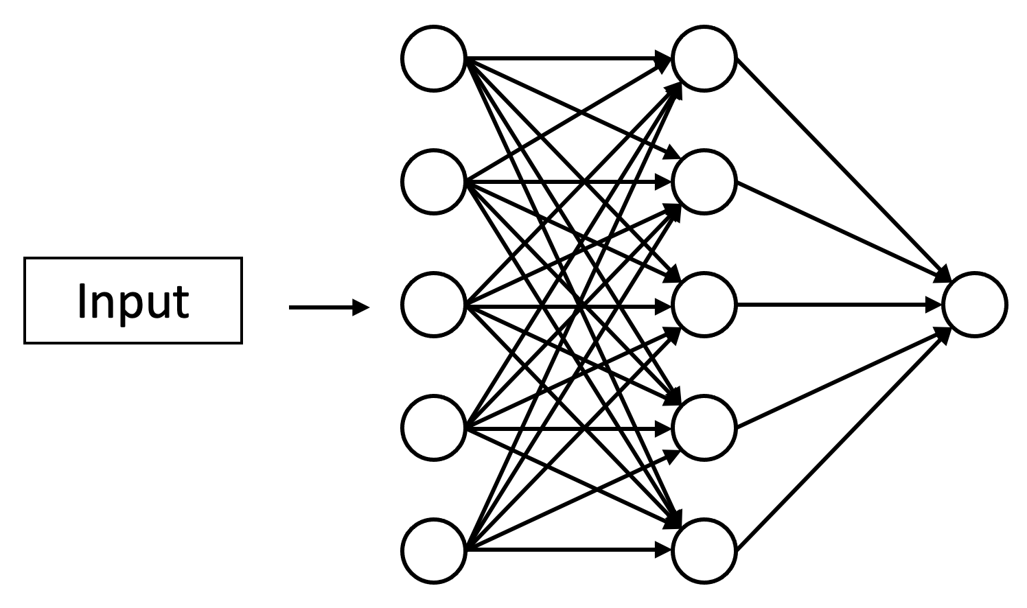
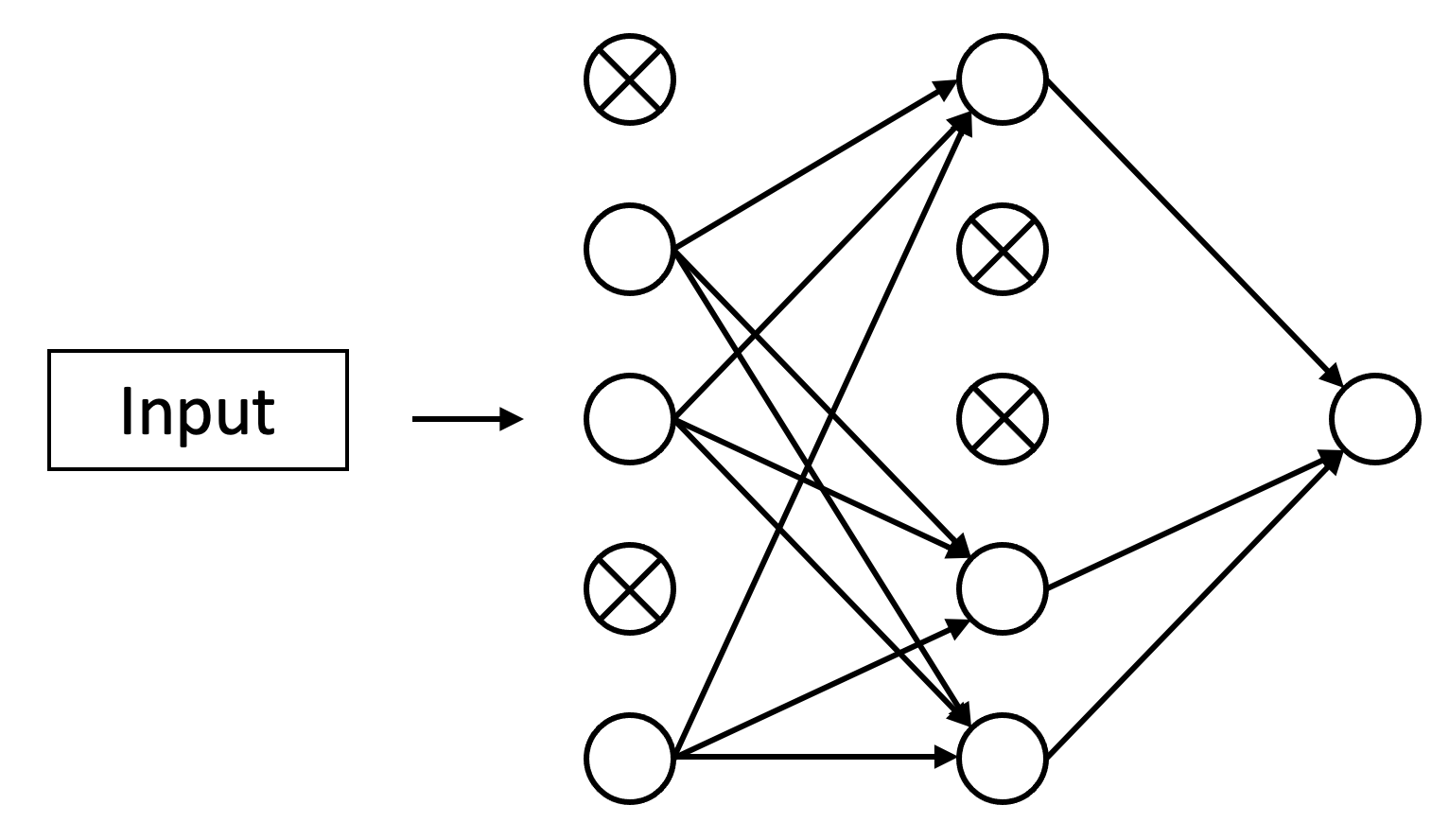

In general, the main idea of these previous works is, while neural networks usually show better performance when going deeper and having more parameters (assuming that there exists a sufficiently large amount of data), they are not necessarily required to use all the neurons to make good predictions, i.e., the activation units in a layer can be sparse. Such sparsity in practice has a regularization effect on over-parameterization. However, most previous works tend to explore specific ways to apply regularization, and use the same regularization pattern over all the input training samples, which may not be optimal because the complexity and variation of input samples are essentially different. For example, distinguishing images of coarse categories, such as dogs vs. cats, is much easier than distinguishing more fine-grained categories, such as two certain species of dogs, because the latter requires learning a more complex combination of visual representations. Thus, another potential way to improve regularization in deep neural networks is to properly allocate the right number of neurons based on each input case, and such a number is just enough for the model to make a correct prediction.
In this work, we aim to explore this regime of keeping essential neurons and dropping out unnecessary ones based on the input data, in order to form simple and powerful representations that generalize well to unseen test cases. An alternative way to view this goal is to generate different network variants that are selected to handle each input sample accordingly, because the samples are likely to require different numbers of neurons to form reasonable representations. Inadequate resources may cause undermined model performance, and on the other hand, overwhelming resources are likely to make the model overfit. As similar problems are well studied in the literature of evolutionary computing (Eiben and Smith, 2003), we consider a novel strategy that evolves selections of neurons to form neural network variants in parallel with the training process of the neural network. The fitness of each network variant is measured by the model performance and the number of neurons used for the prediction. We term this framework Adaptive Neural Selection (ANS), which consists of two parts: a self-attention module and an adaptive regularization mechanism.
The self-attention module is intended to perform selection of neurons by learning a variable weight to be imposed on each neuron. The attention mechanism has been shown in several previous studies (Vaswani et al., 2017; Dai et al., 2019; Hu et al., 2018) to help deep networks focus on essential features and neurons. While the self-attention module can be trained end-to-end in parallel with the neural network through gradient descent, it does not have an objective to adapt neural selection based on the difficulty of predicting each input sample. Thus, we further introduce an adaptive regularization method. This regularization works as a selection pressure that penalizes the self-attention module if it is selecting more neurons than required. The penalization is adaptive to different training samples in regard to the difficulty of performing the task. For example, given a batch of images, if the classification accuracy is low, that means the model has not fully learned good representations of these cases, and thus it is allowed to use more neurons to explore a more complex feature space. The two mechanisms work together to form the Adaptive Neural Selection (ANS) framework, which evolves different sub-network variants by learning the adaptive selection of neurons. ANS can be used on any neural network architecture to adapt its complexity and structure to handle the variety of input cases.
We implement the proposed ANS framework and test it for the image classification task, which is one of the most common tasks for modern deep neural networks. The experiments show that ANS significantly improves commonly-used deep ConvNet architectures on standard benchmarks. On CIFAR-100, ANS improves the test accuracy of ResNet-50 from to , and VGG-16 from to , outperforming Dropout (Srivastava et al., 2014) by a significant margin. Ablation studies also validate that the two components both make a good contribution to the improvement.
In the following sections, we first summarize the related work in the area of machine learning and evolutionary computing. Then we describe the ANS framework and its components. This is followed by experimental results showing the performance of our method. Finally, we conclude by summarizing the results and listing directions for future work.
2. Related Work
Within the broader context of machine learning research, this paper is in line with existing works on regularization methods for neural networks (Yun et al., 2019; DeVries and Taylor, 2017; Gal and Ghahramani, 2016; Huang et al., 2016; Nakkiran et al., 2019; Srivastava et al., 2014; Ghiasi et al., 2018; Pham and Le, 2021; Zoph et al., 2018). Most of the recent methods such as Dropout (Srivastava et al., 2014) and its variants require either specific and careful tuning of the structure based on the datasets or tasks (Ghiasi et al., 2018; Zoph et al., 2018), or expensive computation cost for searching good patterns of regularization (Pham and Le, 2021). Instead of expanding on the current Dropout mechanism, our work explores the problem of regularizing over-parameterization in neural networks from a evolutionary computing perspective. In addition, our work is also related to automated data augmentation (Zoph et al., 2020; Lim et al., 2019; Xie et al., 2019; Cubuk et al., 2018; Li et al., 2020). Unlike most data augmentation methods that are usually applied specifically to the type of input data, our method works on the high-level representations of neural networks. It employs a more general design philosophy, and thus the same mechanism can be easily applied to different data types and tasks.
Our work is inspired by the parent selection methods (Eiben and Smith, 2003; Koza, 1992; Helmuth et al., 2014; La Cava et al., 2019; Aenugu and Spector, 2019; McKay, 2000) in evolutionary computing. More specifically, our method is related to the Implicit Fitness Sharing (McKay, 2000) and Lexicase selection (Helmuth et al., 2014; La Cava et al., 2019; Aenugu and Spector, 2019), in which hard cases are either weighted more heavily in aggregate fitness measures, or required to be correctly predicted by some model variants in every generation, when the training samples are ordered in random sequences. The proposed ANS framework is designed to put selection pressure to guide the neural networks to use the right amount of neurons depending on model performance. Since the neural networks usually require batched training samples to work with large-scale dataset, we follow the general idea in (Aenugu and Spector, 2019) to make the selection framework suitable to be trained with batched samples.
We also take advantage of the attention mechanism, which has been proved to be useful in improving neural network performance with different architectural designs (Vaswani et al., 2017; Dai et al., 2019; Hu et al., 2018) in the context of deep learning. However, most of these methods rely on gradient-based training of the attention layers, in which case the updates of weights in the attention layers are correlated with the updates of weights in the neural network. This will result in co-adaption of weights in both the attention layers and other layers in the neural network, which may still cause overfitting since the network can still learn to memorize all the training samples. On the other hand, our work evolves the self-attention module based on a combination of the proposed adaptive regularization method and gradients from the model prediction loss. In this way, we can prevent the co-adaption of attention and neural network weights, and thus have a stronger regularization effect on the network.
Our work is also closely-connected to prior research on neural evolution (Stanley and Miikkulainen, 2002; Real et al., 2017; Real et al., 2019; Stanley et al., 2009; Miikkulainen et al., 2019), and neural architecture search (Liu et al., 2018a; Pham et al., 2018; Liu et al., 2018b; Cai et al., 2019; Liu et al., 2017). The proposed ANS framework assumes a fixed neural network architecture and evolves different model variants to handle different input cases, which is different from the general neural evolution and architecture search methods that aim to evolve the network architectures. Our method can be further combined with neural evolution methods to co-evolve network variants and network architectures at the same time.
3. Methods
In this section, we introduce the Adaptive Neural Selection (ANS) framework. ANS aims to evolve the behavior of selecting certain neurons from the deep neural networks to perform the prediction task based on the input training samples. The framework consists of two parts: a self-attention module and an adaptive regularization mechanism. An illustration of our method comparing to ordinary neural networks and the Dropout (Srivastava et al., 2014) is shown in Fig. 1.
3.1. Ordinary Neural Network
Consider a neural network with fully connected layers. Let denote the index of hidden layers. Let denote the input vector to layer , and denote the output vector from layer before activation. and are the weight matrix and bias vector at layer . The forward pass operation of an ordinary neural network at layer can be described as
| (1) | ||||
| (2) |
where is the activation function, such as the ReLU function .
The neural network is usually trained using back-propagation and gradient descent. We use to denote the common gradient-based loss functions. For example, the image classification task usually use cross-entropy loss on the one-hot encoded output, described as
| (3) | ||||
| (4) |
where is the one-hot encoded ground truth label in the set of all the training labels, and is the corresponding network’s prediction. The prediction is usually calculated using the softmax function as on the last layer’s output.
For neural networks that have specific layers for feature extraction, such as convolutional neural networks (ConvNets), we also use the above formulation for the fully-connected layers in the network, which usually comes after the feature extraction layers.
3.2. Self-attention Module
To add the self-attention module, we use to denote an attention layer with another pair of weight matrix and bias vector . The forward pass operation of a neural network with attention module can be described as
| (5) | ||||
| (6) | ||||
| (7) |
where is the activation function and is the gating function on the attention weights. In this work, we use the soft attention mechanism which uses the sigmoid function .
By adding the self-attention module, the neuron activations are now regularized by the attention units . Since we have for the sigmoid function, the neurons become selective according to the weights comparing to the ordinary neural network. We can also represent the ordinary neural network with this formulation by having for every neuron, and Dropout can be viewed as having random binary values of . Thus, the self-attention module can achieve a larger space of sub-network structures comparing to Dropout.
While the weight matrix and bias vector for the attention layer can be trained in parallel through normal gradient descent and back-propagation, the resulting selection of neurons may not work well as a regularization for the neural network. As the self-attention module is a fully connected layer extended from the neural network, it may co-adapt with the neural network weight and thus result in overfitting. To solve this issue, we further introduce an adaptive regularization mechanism for the self-attention module, as describe in the next subsection.
3.3. Adaptive Regularization for Neural Selection
In the context of modern deep neural networks, with similar architectures and training protocols, better performance is usually achieved by network variants with deeper structures and parameters. However, the overfitting problem is also more likely to occur especially when training large neural networks with insufficient data. One thing that people usually do not know in advance and thus require lots of experiments and tuning is how many parameters works the best on the given dataset, that will not cause overfitting. A common way to resolve this issue is to have regularization on the neural network, and penalize it for having or relying on too many parameters. For example, Dropout forces the network to only use a random number of neurons, i.e., a sub-network, for prediction during training, and Weight Decay penalizes complexity by adding all the parameters to the loss function.
Most of these methods apply equally to all the training and testing samples, assuming that all the input samples follow the same distribution, and the neural network is trained to work with that distribution. However, some input samples have higher complexity, and thus may need more neurons to form a good representation. To explore this regime, we propose an adaptive regularization mechanism. For layer in the neural network, we use to denote the self-attention units. The regularization is calculated as
| (8) |
where is a variable that controls the extent of regularization and is the number of all the neurons as a normalization factor.
We also introduce a strategy to calculate depending on the model performance on current input samples. The idea is that for better training performance on a batch of data, the chance of overfitting is higher, and we thus need greater regularization to guide the network to use fewer neurons that may form more generalizable representations. To achieve this, we calculate as
| (9) |
where and are hyperparameters controlling the scale and variance of . denotes a non-negative metric of model performance on current input samples. In the context of image classification, for example, we use batch accuracy as the metric where . With this formulation, we have becomes larger when the model performance becomes better, and thus enforcing greater regularization on the neural networks.
3.4. Evolving Adaptive Neural Selection
Here we introduce the Adaptive Neural Selection (ANS) framework that combines the self-attention module and the adaptive regularization method. Inspired by parent selection methods in genetic programming, the ANS framework introduces a selection pressure to the current neural network by injecting regularization on the number of neurons currently being used for the input training sample. By putting the attention weights on a set of neurons for each training sample, the selection actually evolves different sub-network variants adaptively, and such evolution improves as the training process proceeds. The fitness of neuron selection is evaluated by the current model performance, and the way we optimize the neural selection is to select as few neurons as possible depending on the difficulty of predicting the input sample, in order to prevent overfitting on trivial cases or underfitting on hard ones. The full training procedure is described in Algorithm 1.
During the procedure of evolution, the framework trains the neural networks by using a combination of error gradient and regularization. With the help of gradient-based learning, the neural selection can be efficiently optimized and quickly reach convergence. In addition, since most neuroevolutionary methods tends to use non-gradient methods for optimization, such as Gaussian mutation, our framework can be easily extended to apply those techniques as well, by using the term for fitness evaluation. However, in order to show the effectiveness of the proposed framework, we choose to not use those non-gradient optimization methods to ensure fair comparison to the ordinary gradient-trained models.
4. Experiments
In this section, we implement and test the proposed ANS framework to common ConvNet architectures for the supervised image classification task. We compare our method against the Dropout method with different parameter settings. We also perform ablation study on the effect of hyperparameters of ANS.
4.1. ConvNet Architectures
We use the ResNet-50 (He et al., 2016) and VGG-16 (Simonyan and Zisserman, 2014) models for the experiments. Both of the networks are commonly used in various image recognition problems and have been extended to other tasks such as semantic segmentation and object detection. While there are several recent works proposing better performing architectures with novel techniques, we choose to use these two common architectures to better illustrate the performance of our method, which can be further extended to other methods as well.
4.2. Datasets and Metrics
We use the CIFAR-10 and CIFAR-100 datasets (Krizhevsky et al., 2009) for the experiments. The CIFAR-10 dataset consists of 60000 32x32 colour images in 10 classes, with 6000 images per class. There are 50000 training images and 10000 test images. CIFAR-100 has 100 classes containing 600 images each. Similarly, there are 500 training images and 100 testing images per class. The classes are mutually exclusive. Both datasets serve as standard benchmarks for image recognition.
Since both datasets come with a pre-defined testing set, and the classes are well-balanced, we adopt the mean prediction accuracy as the metric.
4.3. Experiment Configuration
We use similar training configurations that are commonly adopted in prior works (DeVries and Taylor, 2017; He et al., 2016). For all the experiments, we use a batch size of and a total number of epoches of . The optimization method is stochastic gradient descent with Nesterov momentum of , with weight decay of . The initial learning rate is for ResNet-50, and for VGG-16, given the fact that VGG-16 has more parameters and thus needs a smaller learning rate to prevent divergence. We decrease the learning rate by a factor of at epoch and for better convergence. All the models are trained from scratch with standard initialization methods as in the original work. We also follow the common data augmentation pipeline in (He et al., 2016), which is random cropping and horizontal flipping. All the training jobs are implemented with PyTorch (Paszke et al., 2019) library and performed on cluster nodes with a single GPU. The test results are obtained on predicting with the single image only, without ensembling.
4.4. Image Classification Results
| Method | CIFAR-10 | CIFAR-100 |
|---|---|---|
| Vanilla ResNet-50 | 0.9418 | 0.7665 |
| Dropout (p = 0.3) | 0.9421 | 0.7587 |
| Dropout (p = 0.5) | 0.9392 | 0.7611 |
| ANS (ours) | 0.9498 | 0.7808 |
| Method | CIFAR-10 | CIFAR-100 |
|---|---|---|
| Vanilla VGG-16 | 0.9046 | 0.6230 |
| Dropout (p = 0.3) | 0.9071 | 0.6455 |
| Dropout (p = 0.5) | 0.9070 | 0.6457 |
| ANS (ours) | 0.9109 | 0.6521 |
We apply the ANS framework on ResNet-50 and VGG-16. For comparison, we also implement the baseline method of the vanilla architectures and add Dropout at rate and . Note that the original implementation of VGG-16 has a default Dropout at , but here for the vanilla VGG-16 we remove the Dropout for fair comparison.
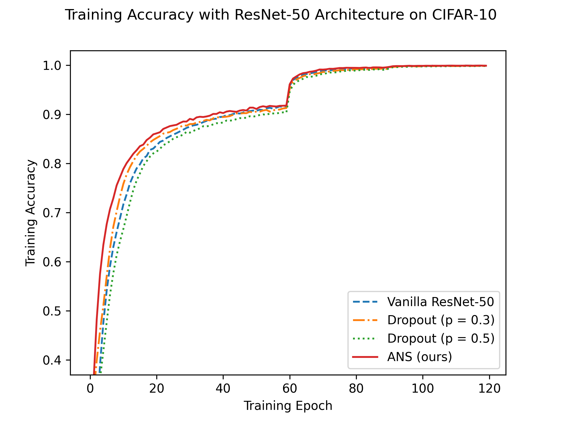
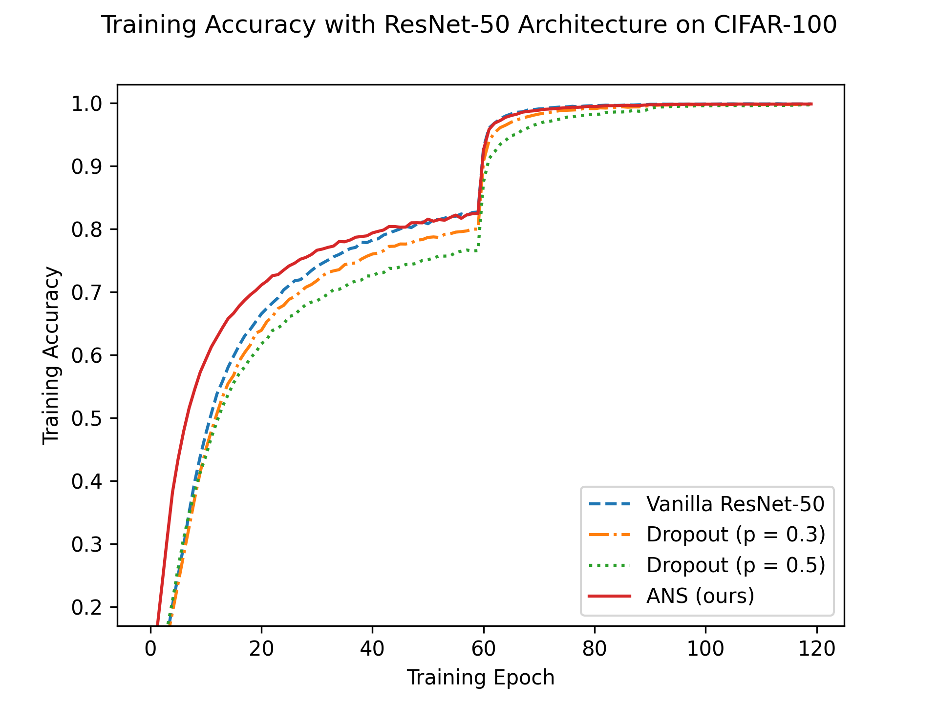
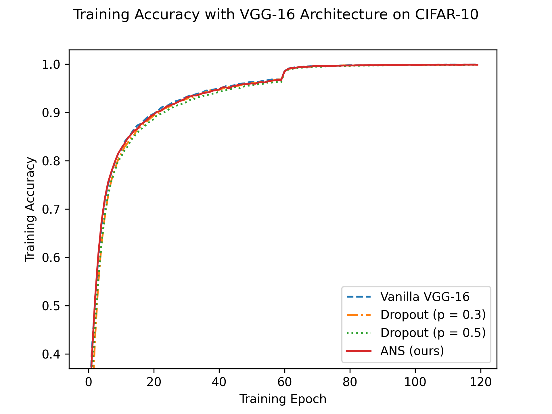
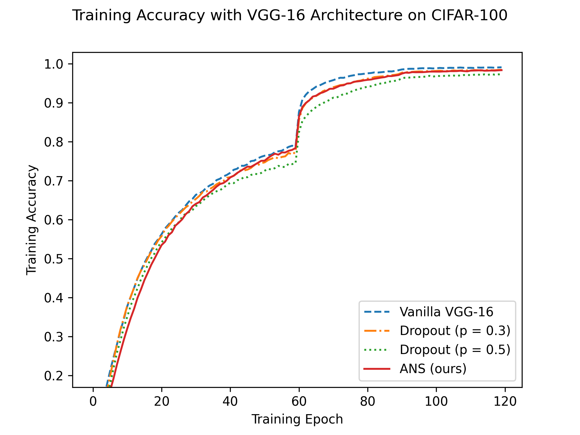
Table 1 shows the test result with ResNet-50 on CIFAR-10 and CIFAR-100. Since the ResNet-50 architecture does not have an intermediate fully connected layer between the feature pooling layer and the classification layer, both Dropout and ANS are applied only on the features layer after average pooling. We can observe that Dropout does not show positive effect on the model performance. However, our ANS method significantly improves the model performance, especially on the harder benchmark CIFAR-100.
For VGG-16, the results are shown in Table 2. Given the VGG-16 architecture, we apply the Dropout and ANS on the last two fully connected layers before the classification layer. The implementation with Dropout rate at 0.5 is identical to the original VGG-16 model. We can first observe that Dropout significantly improves the VGG-16 model, because VGG-16 has more parameters and connection that may be easier to cause overfitting. The proposed ANS method further improves the model performance, outperforming the Dropout method.
One of the drawbacks of methods such as Dropout and its variants is they require specific design and tuning to work with different architectures. For example, (Zaremba et al., 2014) shows that dropping neurons everywhere is not as good as only dropping the neurons in the vertical connections for a multi-layered LSTM network (Hochreiter and Schmidhuber, 1997). Similarly, our results show that even for similar ConvNet architectures, the application of Dropout does not always benefit the model. However, our method consistently improves the neural network despite the underlying architectures and datasets.
4.5. Training Analysis
In Fig. 2, we visualize the training process of the experiments, comparing our method to the vanilla model and Dropout. For ResNet-50, we can observe that with Dropout, the model has similar or slower convergence than the vanilla model. However, our method achieves superior convergence. Since for ResNet-50 the ANS method is directly applied on the final feature representation layer after the pooling operation, it is able to improve the learning process by putting more effort on the difficult cases. This is because the selection pressure limits the usage of neurons for easier cases, and thus the loss on difficult cases has larger weight on the network updates.
For the VGG-16 model, while we can still observe that the convergence of ANS is slightly better than Dropout, the vanilla model actually converges faster. Considering the fact that the vanilla VGG-16 has significantly worse testing performance than using Dropout and ANS (as shown in Table 2), we can see that the vanilla VGG-16 easily overfits the training data if no regularization method is used. This is because VGG-16 has many more parameters within the last two fully connected layers. Regarding the complexity of the VGG-16 model, while the convergence speed is similar, ANS improves the generalization capability of VGG-16 with little cost on the training process.
| Method | CIFAR-10 | CIFAR-100 |
|---|---|---|
| Vanilla ResNet-50 | 0.9418 | 0.7665 |
| ANS (self-attention only) | 0.9467 | 0.7700 |
| ANS (full) | 0.9498 | 0.7808 |
| Method | CIFAR-10 | CIFAR-100 |
|---|---|---|
| Vanilla VGG-16 | 0.9046 | 0.6230 |
| ANS (self-attention only) | 0.9088 | 0.6360 |
| ANS (full) | 0.9109 | 0.6521 |
In addition, since CIFAR-10 has fewer classes and more data for each class, it is usually easier to work with than CIFAR-100. Most of the analysis and results are better illustrated on CIFAR-100.
4.6. Ablation Study
To further validate the effectiveness of the proposed ANS method, we perform ablation study on the components and hyperparameters of ANS. The experiment settings are identical to the experiments in previous sections, where we test ANS with ResNet-50 and VGG-16 on both CIFAR-10 and CIFAR-100.
4.6.1. Effectiveness of Components
The proposed ANS framework consists of two components: the self-attention module and the adaptive regularization loss. In this ablation study, we validate the effectiveness of each components by having the test setting that removes the adaptive regularization loss by letting , meaning the self-attention module is trained only using gradients from the classification loss, without the adaptive regularization. The results are shown in Table 3 and Table 4.
We can first observe that with the self-attention module only, ANS is able to improve the model performance by an obvious margin. Similar results have been shown in some recent works (Hu et al., 2018; Vaswani et al., 2017) that utilize attention-like mechanism in tuning deep neural network architectures.
Secondly, by adding the adaptive regularization, the performance is further improved to a larger extent. For example, the testing accuracy is boosted by by adding adaptive regularization to the self-attention-only ResNet-50, while the self-attention itself adds to the vanilla model. The results shows that the adaptive regularization mechanism is able to evolve better neural selections comparing to just using end-to-end gradient training.
4.6.2. Hyperparameters
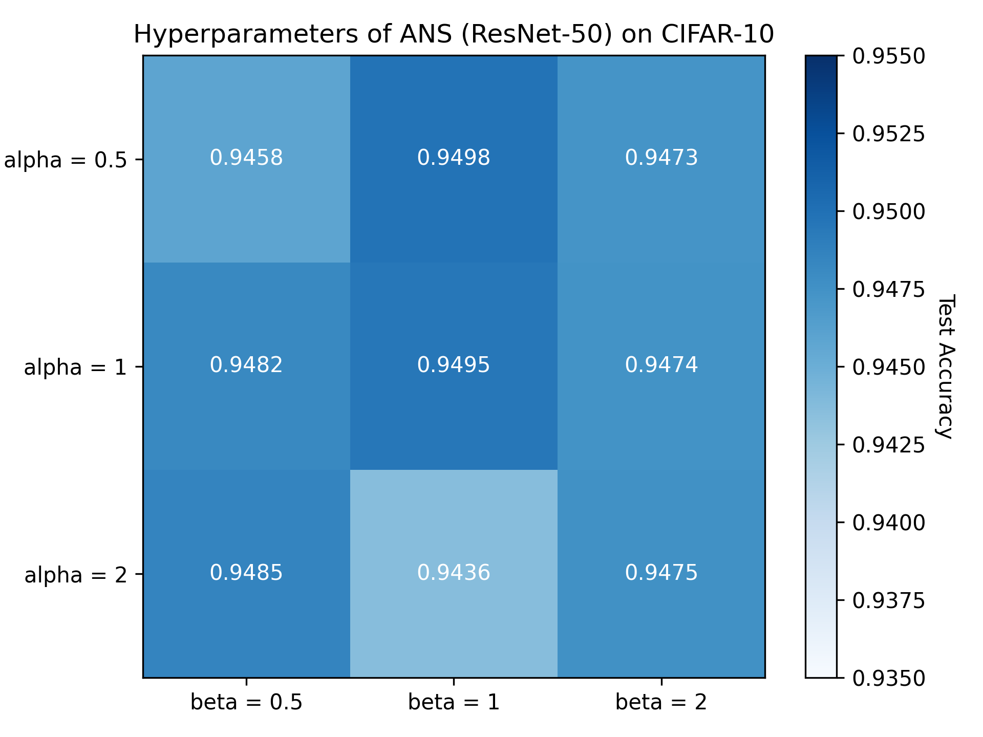
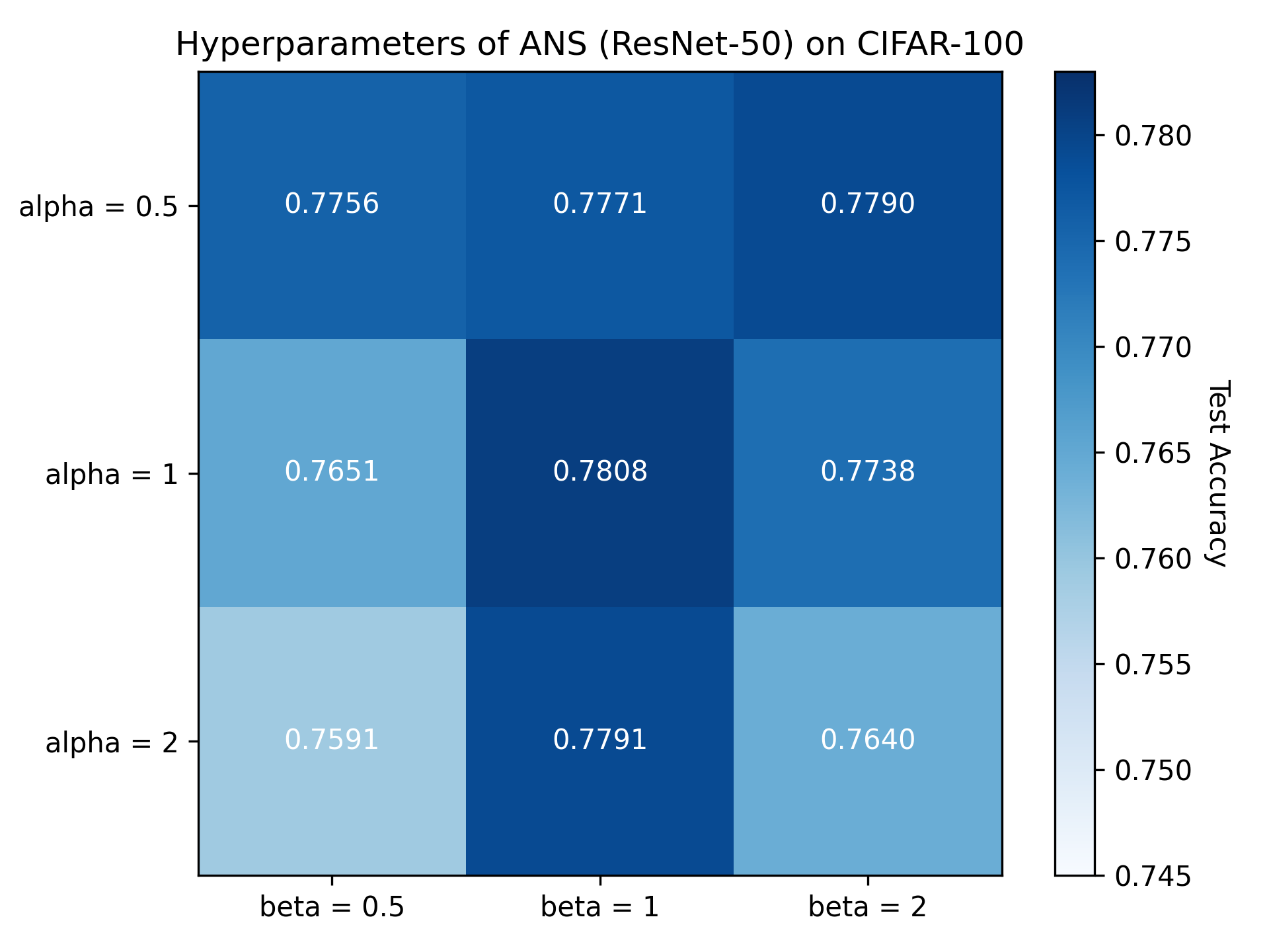
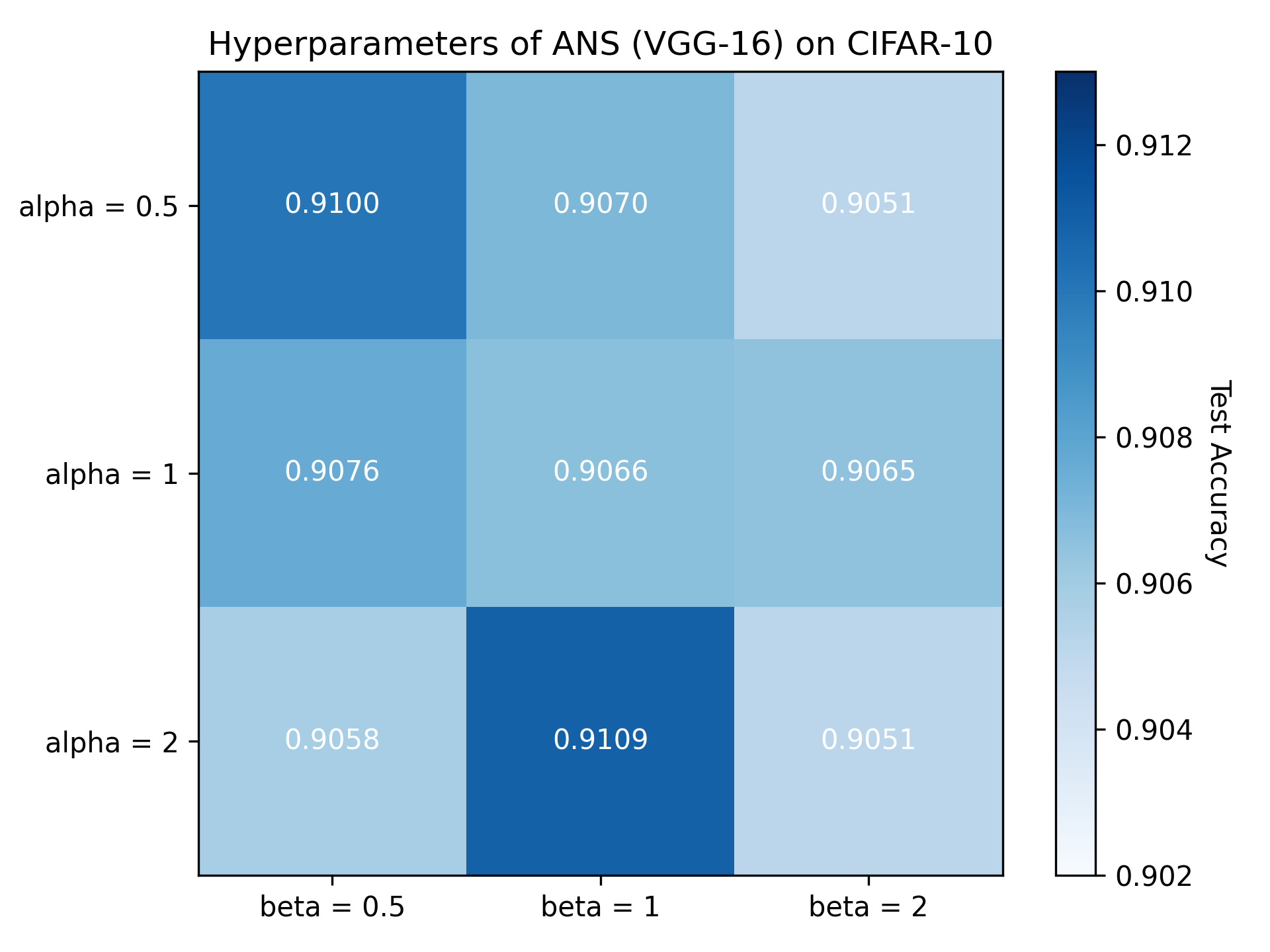
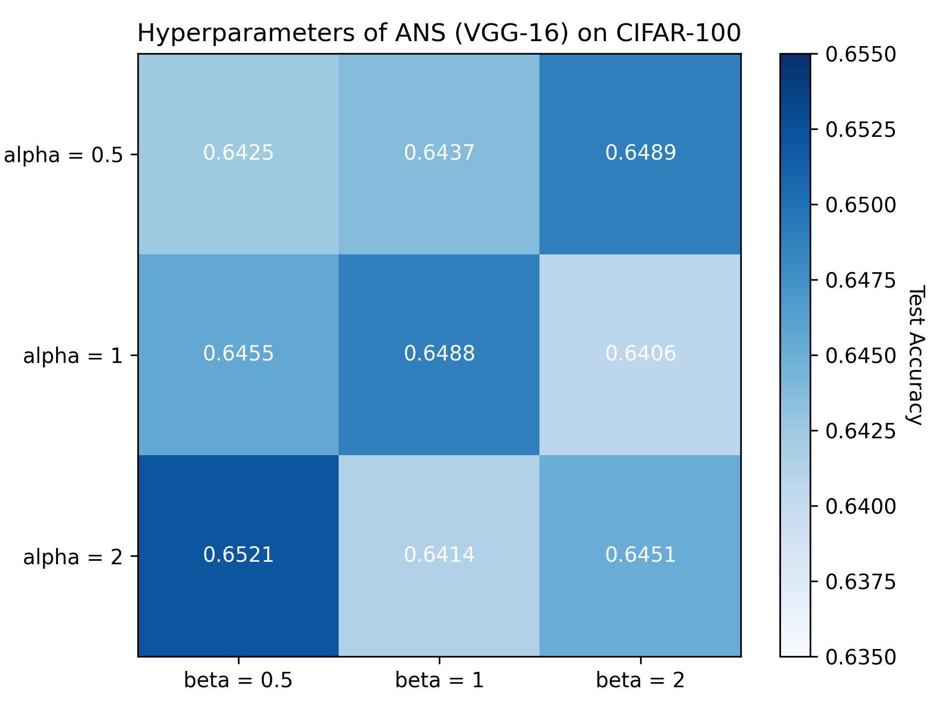
The fitness function of neural selection is controlled by two hyperparameters: and , as stated in Eq. 9. We investigate how different hyperparameter settings may influence the model performance with ANS, as the selection pressure is tuned by changing them. Fig. 3 shows the testing results on different and settings in the format of heatmaps with the exact accuracy number in each cell. In order to properly weigh the two losses for joint learning, we limit the scale of searching space of and by having and . We test for every combination of the two hyperparameters within this space.
In general, we can see that the framework is relatively robust to different hyperparameters settings. For example, for the ResNet-50 model on CIFAR-100, the worst-performing hyperparameter setting () has testing accuracy , which is still higher than using Dropout() which has accuracy .
While there is no obvious pattern and correlation in terms of the hyperparameters, it should be noted that the hyperparameters of ANS can be problem dependent, just like hyperparameters for other selection methods in evolutionary computing (such as the tournament size parameter for tournament selection). However, we found that a setting of and has been robust for most of the cases.
5. Conclusion and Future Work
In this paper, we propose the Adaptive Neural Selection (ANS) method and a framework for deep neural networks to evolve the behavior of selecting specific neurons from the networks to perform the prediction task adaptively based on the current input data. ANS can significantly improve the model performance on generalization to unseen test cases without slowing down the training process. Ablation study also shows that ANS has robust performance over different hyperparameter settings.
While this work only applies ANS on fully-connected layers, ANS can be easily extended to other network architectures, such as convolutional layers, by transforming it to variants with specific structures. ANS can also be optimized by using non-gradient neuroevolutionary techniques, which may further improve the evolution of its weights.
In addition, while we keep the basic network architecture unchanged and only evolve the selection of neurons, the ANS framework can also be used to evolve the network architectures, serving as a strategy for neural architecture search. For example, instead of putting regularization on attention weights, we can alternatively use ANS to regularize the complexity of the network architecture by removing layers, connections, etc. We look forward to a deeper analysis on the effectiveness of combining ANS with other neural network evolution strategies.
Acknowledgements.
This material is based upon work supported by the National Science Foundation under Grant No. 1617087. Any opinions, findings, and conclusions or recommendations expressed in this publication are those of the authors and do not necessarily reflect the views of the National Science Foundation. This work was performed in part using high performance computing equipment obtained under a grant from the Collaborative R&D Fund managed by the Massachusetts Technology Collaborative. The authors would like to thank Edward Pantridge, Anil Kumar Saini, and Dr. Thomas Helmuth for their valuable comments and helpful suggestions.References
- (1)
- Aenugu and Spector (2019) Sneha Aenugu and Lee Spector. 2019. Lexicase selection in learning classifier systems. In Proceedings of the Genetic and Evolutionary Computation Conference. 356–364.
- Cai et al. (2019) Han Cai, Ji Lin, Yujun Lin, Zhijian Liu, Kuan Wang, Tianzhe Wang, Ligeng Zhu, and Song Han. 2019. Automl for architecting efficient and specialized neural networks. IEEE Micro 40, 1 (2019), 75–82.
- Cubuk et al. (2018) Ekin D Cubuk, Barret Zoph, Dandelion Mane, Vijay Vasudevan, and Quoc V Le. 2018. Autoaugment: Learning augmentation policies from data. arXiv preprint arXiv:1805.09501 (2018).
- Dai et al. (2019) Zihang Dai, Zhilin Yang, Yiming Yang, Jaime Carbonell, Quoc V Le, and Ruslan Salakhutdinov. 2019. Transformer-xl: Attentive language models beyond a fixed-length context. arXiv preprint arXiv:1901.02860 (2019).
- DeVries and Taylor (2017) Terrance DeVries and Graham W Taylor. 2017. Improved regularization of convolutional neural networks with cutout. arXiv preprint arXiv:1708.04552 (2017).
- Eiben and Smith (2003) A. E. Eiben and J. E. Smith. 2003. Introduction to Evolutionary Computing. Springer. https://doi.org/doi:10.1007/978-3-662-44874-8
- Gal and Ghahramani (2016) Yarin Gal and Zoubin Ghahramani. 2016. Dropout as a bayesian approximation: Representing model uncertainty in deep learning. In international conference on machine learning. PMLR, 1050–1059.
- Ghiasi et al. (2018) Golnaz Ghiasi, Tsung-Yi Lin, and Quoc V Le. 2018. Dropblock: A regularization method for convolutional networks. arXiv preprint arXiv:1810.12890 (2018).
- He et al. (2016) Kaiming He, Xiangyu Zhang, Shaoqing Ren, and Jian Sun. 2016. Deep residual learning for image recognition. In Proceedings of the IEEE conference on computer vision and pattern recognition. 770–778.
- Helmuth et al. (2014) Thomas Helmuth, Lee Spector, and James Matheson. 2014. Solving uncompromising problems with lexicase selection. IEEE Transactions on Evolutionary Computation 19, 5 (2014), 630–643.
- Hochreiter and Schmidhuber (1997) Sepp Hochreiter and Jürgen Schmidhuber. 1997. Long short-term memory. Neural computation 9, 8 (1997), 1735–1780.
- Hu et al. (2018) Jie Hu, Li Shen, and Gang Sun. 2018. Squeeze-and-excitation networks. In Proceedings of the IEEE conference on computer vision and pattern recognition. 7132–7141.
- Huang et al. (2016) Gao Huang, Yu Sun, Zhuang Liu, Daniel Sedra, and Kilian Q Weinberger. 2016. Deep networks with stochastic depth. In European conference on computer vision. Springer, 646–661.
- Koza (1992) John R. Koza. 1992. Genetic Programming: On the Programming of Computers by Means of Natural Selection. MIT Press, Cambridge, MA, USA. http://mitpress.mit.edu/books/genetic-programming
- Krizhevsky et al. (2009) Alex Krizhevsky, Geoffrey Hinton, et al. 2009. Learning multiple layers of features from tiny images. (2009).
- La Cava et al. (2019) William La Cava, Thomas Helmuth, Lee Spector, and Jason H. Moore. 2019. A probabilistic and multi-objective analysis of lexicase selection and epsilon-lexicase selection. Evolutionary Computation 27, 3 (Fall 2019), 377–402. https://doi.org/doi:10.1162/evco_a_00224
- Li et al. (2020) Boyi Li, Felix Wu, Ser-Nam Lim, Serge Belongie, and Kilian Q Weinberger. 2020. On feature normalization and data augmentation. arXiv preprint arXiv:2002.11102 (2020).
- Lim et al. (2019) Sungbin Lim, Ildoo Kim, Taesup Kim, Chiheon Kim, and Sungwoong Kim. 2019. Fast autoaugment. arXiv preprint arXiv:1905.00397 (2019).
- Liu et al. (2018b) Chenxi Liu, Barret Zoph, Maxim Neumann, Jonathon Shlens, Wei Hua, Li-Jia Li, Li Fei-Fei, Alan Yuille, Jonathan Huang, and Kevin Murphy. 2018b. Progressive neural architecture search. In Proceedings of the European conference on computer vision (ECCV). 19–34.
- Liu et al. (2017) Hanxiao Liu, Karen Simonyan, Oriol Vinyals, Chrisantha Fernando, and Koray Kavukcuoglu. 2017. Hierarchical representations for efficient architecture search. arXiv preprint arXiv:1711.00436 (2017).
- Liu et al. (2018a) Hanxiao Liu, Karen Simonyan, and Yiming Yang. 2018a. Darts: Differentiable architecture search. arXiv preprint arXiv:1806.09055 (2018).
- McKay (2000) R I (Bob) McKay. 2000. Fitness Sharing in Genetic Programming. In Proceedings of the Genetic and Evolutionary Computation Conference (GECCO-2000), Darrell Whitley, David Goldberg, Erick Cantu-Paz, Lee Spector, Ian Parmee, and Hans-Georg Beyer (Eds.). Morgan Kaufmann, Las Vegas, Nevada, USA, 435–442. http://gpbib.cs.ucl.ac.uk/gecco2000/GP256.pdf
- Miikkulainen et al. (2019) Risto Miikkulainen, Jason Liang, Elliot Meyerson, Aditya Rawal, Daniel Fink, Olivier Francon, Bala Raju, Hormoz Shahrzad, Arshak Navruzyan, Nigel Duffy, et al. 2019. Evolving deep neural networks. In Artificial intelligence in the age of neural networks and brain computing. Elsevier, 293–312.
- Nakkiran et al. (2019) Preetum Nakkiran, Gal Kaplun, Yamini Bansal, Tristan Yang, Boaz Barak, and Ilya Sutskever. 2019. Deep double descent: Where bigger models and more data hurt. arXiv preprint arXiv:1912.02292 (2019).
- Paszke et al. (2019) Adam Paszke, Sam Gross, Francisco Massa, Adam Lerer, James Bradbury, Gregory Chanan, Trevor Killeen, Zeming Lin, Natalia Gimelshein, Luca Antiga, et al. 2019. Pytorch: An imperative style, high-performance deep learning library. arXiv preprint arXiv:1912.01703 (2019).
- Pham et al. (2018) Hieu Pham, Melody Guan, Barret Zoph, Quoc Le, and Jeff Dean. 2018. Efficient neural architecture search via parameters sharing. In International Conference on Machine Learning. PMLR, 4095–4104.
- Pham and Le (2021) Hieu Pham and Quoc V Le. 2021. AutoDropout: Learning Dropout Patterns to Regularize Deep Networks. arXiv preprint arXiv:2101.01761 (2021).
- Real et al. (2019) Esteban Real, Alok Aggarwal, Yanping Huang, and Quoc V Le. 2019. Regularized evolution for image classifier architecture search. In Proceedings of the aaai conference on artificial intelligence, Vol. 33. 4780–4789.
- Real et al. (2017) Esteban Real, Sherry Moore, Andrew Selle, Saurabh Saxena, Yutaka Leon Suematsu, Jie Tan, Quoc V Le, and Alexey Kurakin. 2017. Large-scale evolution of image classifiers. In International Conference on Machine Learning. PMLR, 2902–2911.
- Simonyan and Zisserman (2014) Karen Simonyan and Andrew Zisserman. 2014. Very deep convolutional networks for large-scale image recognition. arXiv preprint arXiv:1409.1556 (2014).
- Srivastava et al. (2014) Nitish Srivastava, Geoffrey Hinton, Alex Krizhevsky, Ilya Sutskever, and Ruslan Salakhutdinov. 2014. Dropout: a simple way to prevent neural networks from overfitting. The journal of machine learning research 15, 1 (2014), 1929–1958.
- Stanley et al. (2009) Kenneth O Stanley, David B D’Ambrosio, and Jason Gauci. 2009. A hypercube-based encoding for evolving large-scale neural networks. Artificial life 15, 2 (2009), 185–212.
- Stanley and Miikkulainen (2002) Kenneth O Stanley and Risto Miikkulainen. 2002. Evolving neural networks through augmenting topologies. Evolutionary computation 10, 2 (2002), 99–127.
- Vaswani et al. (2017) Ashish Vaswani, Noam Shazeer, Niki Parmar, Jakob Uszkoreit, Llion Jones, Aidan N Gomez, Lukasz Kaiser, and Illia Polosukhin. 2017. Attention is all you need. arXiv preprint arXiv:1706.03762 (2017).
- Xie et al. (2019) Qizhe Xie, Zihang Dai, Eduard Hovy, Minh-Thang Luong, and Quoc V Le. 2019. Unsupervised data augmentation for consistency training. arXiv preprint arXiv:1904.12848 (2019).
- Yun et al. (2019) Sangdoo Yun, Dongyoon Han, Seong Joon Oh, Sanghyuk Chun, Junsuk Choe, and Youngjoon Yoo. 2019. Cutmix: Regularization strategy to train strong classifiers with localizable features. In Proceedings of the IEEE/CVF International Conference on Computer Vision. 6023–6032.
- Zaremba et al. (2014) Wojciech Zaremba, Ilya Sutskever, and Oriol Vinyals. 2014. Recurrent neural network regularization. arXiv preprint arXiv:1409.2329 (2014).
- Zoph et al. (2020) Barret Zoph, Ekin D Cubuk, Golnaz Ghiasi, Tsung-Yi Lin, Jonathon Shlens, and Quoc V Le. 2020. Learning data augmentation strategies for object detection. In European Conference on Computer Vision. Springer, 566–583.
- Zoph et al. (2018) Barret Zoph, Vijay Vasudevan, Jonathon Shlens, and Quoc V Le. 2018. Learning transferable architectures for scalable image recognition. In Proceedings of the IEEE conference on computer vision and pattern recognition. 8697–8710.