Classical Yang Mills equations with sources: consequences of specific scalar potentials

Abstract

Some well known gauge scalar potential very often considered or used in the literature are investigated by means of the classical Yang Mills equations for the $SU(2)$ subgroups of $N_{c}=3$. By fixing a particular shape for the scalar potential, the resulting vector potentials and the corresponding color-charges sources are found. By adopting the spherical coordinate system, it is shown that spherically symmetric solutions, only dependent on the radial coordinate, are only possible for the Abelian limit, otherwise, there must have angle-dependent component(s). The following solutions for the scalar potential are investigated: the Coulomb potential and a non-spherically symmetric generalization, a linear potential $A_{0}(\vec{r})\sim(\kappa r)$, a Yukawa-type potential $A_{0}(\vec{r})\sim(Ce^{-r/r_{0}}/r)$ and finite spatial regions in which the scalar potential assumes constant values. The corresponding chromo-electric and chromo-magnetic fields, as well as the color-charge densities, are found to have strong deviations from the spherical symmetric configurations. We speculate these types of non-spherically symmetric configurations may contribute (or favor) for the (anisotropic) confinement mechanism since they should favor color charge-anti-charge (or three-color-charge) bound states that are intrinsically non spherically symmetric with (asymmetric) confinement of fluxes. Specific conditions and relations between the parameters of the solutions are also presented.

1 Introduction

The Classical Yang-Mills Lagrangian [1] corresponds to the leading lower dimension local gauge-invariant terms for a Lorentz covariant description of non-Abelian gauge-potentials. It provided an important framework for the development of the Standard Model (SM) in which non-Abelian gauge fields are at the basis of both Electroweak Model and Quantum Chromodynamics (QCD) for the strong interactions [2, 3, 4]. The strong interactions sector is formulated with the color group $SU(N_{c}=3)$ with eight four-vector potentials $A_{\mu}^{a}$ ($a=1,...N_{c}^{2}-1$), for three color charges of the fundamental representation, being, therefore, the number of degrees of freedom considerably large. The complicated non-Abelian structure of the Yang-Mills fields makes it difficult to be solved already at the classical level and still more difficult at the quantum level. Despite the need and importance of the quantum field description of the strong interactions, classical configurations in Yang-Mills (YM) theories have been proved to be of interest for both, QCD and the SM, also with Landau-Ginzburg/Abelian-Higgs models. Standard monopolar or dipolar configurations of the chromo-electromagnetic fields have been found either in Minkowski or Euclidean space-times, for example in Refs. [5, 6, 7]. Besides their eventual roles in particular physical situations, as discussed below, some of these classical solutions, in Euclidianized spacetime, have been shown to be relevant, for example, in lattice QCD simulations, that is the case of instantons [8, 9, 10]. At least, one might expect that solutions for the classical YM theory might help to gain some insights for the more complete quantum system. Very often scalar gauge potentials, sometimes obtained from lattice QCD, are plugged into quark-bound state equations, either Dirac equation or Schrodinger equation for heavy hadrons, to provide predictions for hadron spectroscopy, for example [11, 12]. It turns out to be interesting to verify if the use of these scalar gauge potentials would bring further consequences or requirements when analyzed from the point of view of the YM theory, such as the classical YM equations. The first step of this program is carried out in this work.

Besides an initial interest in finding solutions of pure Yang-Mills theory, their coupling to fermion sources, quarks, are also needed. The investigation of the equations of motion have been already considered as a sort of first framework for these problems. Different approaches for solving the equations of motion have been developed [13, 14, 15, 16, 20, 21] since the first investigations [1, 22]. The usual Coulomb solution, an Abelian solution, is recovered in the non-Abelian limit of the full theory as a particular limit. Many solutions for the YM equations with sources that have smaller energies than the Coulomb potential have also been found, for example in [13, 16] and fluctuations around the Coulomb solution with conditions for their stability have been found earlier for example in [15]. The effects of different color-charge distributions with particular symmetries have been analyzed within different specific conditions such as for cylinder color-distribution shape [52], plane color distribution [51] and dynamical color-current as sources [53]. Some finite energy conditions for the Yang-Mills equations were formulated by S. Coleman and others by assuming that gauge fields go asymptotically to constant values [6]. Constant gauge potential configurations have been envisaged both in classical and quantum calculations [40, 24] with resulting instabilities already known from the Abelian case. Although some celebrated solutions have constant chromomagnetic fields [25], a realistic vacuum however cannot possess either constant gauge potential nor constant $F_{\mu\nu}$ and, in general, the QCD ground state is believed to have neither $E_{c}$ nor $B_{c}$, chromo-electric and chromo-magnetic fields, equal to zero [26]. Given the large number of degrees of freedom, several different simplifying (symmetric) limits and situations have been considered and some general properties have been determined at the classical level. Among the several earlier works, the papers by by Sikivie and Weiss [13, 14] were considered as a partial guide for the present work, with different configurations for monopole and dipole-type color-charge. To what extent classical configurations are stable or survive in the quantum description is of course extremely important, although it may be interesting by itself to trace back each effect of the realistic exact solution to eventual classical or quantum origin(s).

Despite the more general interest in determining the gauge field dynamics by starting from the classical description, there might have different situations in which classical gauge configurations have been argued or shown to play specific or important roles. Possible effects of (semi)classical configurations of the gluon field on hadrons structure have been investigated for heavy quarkonia in [27]. Classical gluon fields are also expected to contribute in the initial conditions of relativistic heavy-ion collisions when gluons should be copiously produced being the occupation number so high that they may be treated classically, for example in Ref. [28]. The stability of fast varying classical configurations becomes important [29]. Although static solutions may be considered as initial conditions for such time evolution, the time dependence is extremely important [30] and it usually involves non-equilibrium situations [31]. The corresponding (classical) shear viscosity was calculated in [32]. Confinement is one of the most intriguing problems in Physics and its description in the quantum regime still presents several difficulties. One can try to understand, nevertheless, to what extent classical gauge field configurations can mimic, favor, or be associated to the full confining gauge field solutions. The pure Yang-Mills theory, in three dimensions, has been shown to provide confinement classically [33]. A linear increase of the gauge scalar potential is the basis of one of the currently investigated mechanisms of confinement in four space-time dimensions, the dual superconductor confinement mechanism [34]. Quantum calculations in lattice QCD lead to a linear potential as well as a (screened) Coulomb-type solution. These well known solutions, sometimes considered as simple Abelian limiting cases, are very often considered in the literature to be plugged into dynamical or bound state equations to provide hadron spectroscopy. In the present work we intend to provide a more dynamical framework which may help to extend such phenomenological potentials. When they are considered, they can be expected to have corresponding vector potentials and color-charge distributions at the classical Yang-Mills equations level. since color degrees of freedom do not show up outside hadrons. Besides that, it is interesting to note that in confined systems, i.e. mesons and baryons [35, 36, 37], these chromo-electromagnetic fluxes must not be spherically symmetric unless some sort of dynamical rotation restores spherical symmetry in the system, being, therefore, time-dependent.

In the present work new time-independent solutions for the classical YM equations in the presence of punctual and extended sources are presented. Not only the Euler-Lagrange equations are considered, but also the constraint-like Jacobi equations. Although the problem is formulated for $SU(N_{c}=3)$ the equations for the $SU(2)$ subgroups will be solved. After the proper alignment of color charges, as presented in Ref. [13] we find that there must have no fully spherically symmetric non-Abelian solutions simultaneously for the scalar and vector potentials as defined below, i.e. $A_{0}(\vec{r})=A_{0}(r)$ and $\vec{A}(\vec{r})=\vec{A}(r)$. Given a necessary anisotropy, the logics of the work is basically to require a particular known shape for (spherically symmetric) scalar potential and to verify how the color charge distribution and vector potential must behave to ensure those specific scalar potential solutions. This type of procedure can be also thought as a (classical) verification of situations in which Coulomb potential makes sense. For that, the following scalar potentials will be considered: the Coulomb potential and an asymmetric generalization, a linear potential that may be expected to partially mimics a confinement potential, and an Yukawa potential. Besides that, finite spatial regions with constant scalar potential are also considered. The resulting corresponding vector potentials and the color-charge distribution contain strong spatial anisotropies. Also, phenomenological interpretation of some solutions are eventually provided by means of classical models of interest for general aspects of hadrons. Many cases of instabilities of a uniform electric field in classical Abelian and non-Abelian YM were found such as in Refs. [38, 39, 40]. Therefore, in general, we chose the boundary conditions for the chromo-electromagnetic fields to go asymptotically to zero. The work is organized as follows. In the next section the equations for the $SU(N_{c}=3)$ case, and the equations for the $SU(N_{c}=2)$ subgroups, are presented and particular limits for which the equations reduce to the Abelian equations are identified. In section (3) it is shown that there cannot have a fully spherically symmetric solution for both scalar and vector potentials. In section (4) the scalar potential is fixed to be a Coulomb potential and the resulting vector potential, with a corresponding color-charge density, that allows such configuration are found. Next, in section (5) a particular non-spherical generalization of the Coulomb potential will be considered and the corresponding vector potentials and charge distributions found also analytically. In section (6) the scalar gauge potential is fixed to be a linear one, $\kappa r$. The corresponding vector potential, chromo-electric and chromo-magnetic fields and needed color charge distributions are found analytically from the equations. The scalar potential is considered to be a Yukawa type potential in section (7), and the corresponding vector potentials are found numerically. The typical length of the Yukawa potentials is traced back to a color-charge distribution size, out of which gauge vector fields disappear. Finally, a specific case of constant gauge field solution is proposed to be valid within a very specific finite spatial regions in section (8). The constant scalar potentials is kept inside two semi-spheres of radius $R$ in a dipole-type configuration (positive and negative). The corresponding color charge-anticharge sources are distributed inside a sphere that might be modeled by two quarks of color charge and two anti-quarks of anti-color charge, and it is considered as a classical (relativistic) model to describe masses and radii of heavy tetraquarks. The corresponding vector potentials and color-charge distribution are found analytically. Finally, in the last section, there is a summary with conclusions.

2 Classical Yang Mills equations with sources - $N_{c}=3$

The Yang-Mills Lagrangian corresponds to the leading (lower dimension) gauge-invariant terms for gauge fields, $A_{\mu}^{a}(x)$, displayed according to the compact Lie group SU($N_{c}$). Classical Chromodynamics (CCD) is obtained by adding a gauge invariant coupling with quark sources and the corresponding free terms. It yields:

$${\cal L} = \bar{\psi}\left(iD\cdot\gamma-m\right)\psi-\frac{1}{4}F_{\mu\nu}^{a}F^{\mu\nu}_{a},$$ (1)

where $\psi$ is the quark field and its mass $m$ can be taken to be an unique flavor state of the SU($N_{f}$) fundamental representation for $N_{f}$ flavors, and the three states for SU($N_{c}=3$) in the fundamental representation. $a=1,...,(N_{c}^{2}-1)$ are indices for color in the adjoint representation, The (gauge invariant) covariant derivative, that can be considered a basic way to build up gauge invariant quantities, is given by:

$$D_{\mu} = \partial_{\mu}-iA_{\mu}g,$$ (2)

where $A_{\mu}=A_{\mu}^{a}\cdot\lambda^{a}$, being $\lambda_{a}$ the GellMann matrices as the generators of the algebra, and the (gauge invariant) non-Abelian stress tensor has been defined as:

$$F_{\mu\nu} = \partial_{\mu}A_{\nu}-\partial_{\nu}A_{\mu}-ig[A_{\mu},A_{\nu}].$$ (3)

A finite gauge transformation for this gauge field can be written as:

$$A_{\mu}(x)\to A_{\mu}^{U}(x)=\partial_{\mu}U(x)U^{-1}(x)+U(x)A_{\mu}U^{-1}(x),$$ (4)

where the algebra element can be written in terms of a closed path C in a path ordering operator:

$$U(C;A)=P\;exp\left(\int_{C}A(x)\cdot dx\right).$$ (5)

The (color) Noether current is given by

$$J^{\mu}=j^{\mu}-ig[A_{\nu},F^{\nu\mu}]=\partial_{\nu}F^{\nu\mu},$$ (6)

where the quark currents can be written shortly, for $j_{a}^{\mu}\cdot\lambda_{a}=j^{\mu}$, as:

$$j_{a}^{\mu}=\bar{\psi}\gamma^{\mu}\lambda_{a}\psi.$$ (7)

being that

$$D_{\mu}J^{\mu}=\partial_{\mu}j^{\mu}+ig[A_{\mu},j^{\mu}]=0.$$ (8)

2.1 Dynamical equations

The Euler-Lagrange equations for the gluon field can be written as:

$$D_{\mu}F^{\mu\nu}=\partial_{\mu}F^{\mu\nu}-ig[A_{\mu},F^{\mu\nu}]=j^{\nu}.$$ (9)

These equations can be reduced to the non-Abelian versions of electric Gauss’s law and the Ampère-Maxwell equations. Also, to present a set of equations with clear correspondence with the Maxwell equations of electromagnetism, the Jacobi identity must also be considered. It can be written as:

$$D_{\rho}F^{\mu\nu}+D_{\mu}F^{\nu\rho}+D_{\nu}F^{\rho\mu}=0.$$ (10)

Due to the anti-symmetry of $F_{\mu\nu}$, these equations can be written as two equations that correspond to non-Abelian generalizations of the magnetic Gauss’s law and the Faraday equation, both discussed below.

For the time independent gauge potentials, i.e. $\partial_{t}A_{\mu}=0$, the Euler Lagrange equations (9) and the equations obtained from the Jacobi identity (10) can be written as:

$$-J^{0}_{a} = \nabla^{2}A^{0}_{a}-gf_{abc}\left(\vec{\nabla}\cdot\vec{A}_{b}\right)A^{0}_{c}+g^{2}f_{abc}f_{cde}\vec{A}_{b}\cdot\vec{A_{d}}A^{0}_{e};$$ (11)

$$0 = gf_{abc}\left(\vec{\nabla}\times\vec{A}_{b}\cdot\vec{A}_{c}-3\vec{A}_{b}\cdot\vec{\nabla}\times\vec{A}_{c}-gf_{cde}\vec{A}_{b}\cdot\left(\vec{A}_{d}\times\vec{A}_{e}\right)\right);$$ (12)

$$0 = gf_{abc}\left(\vec{\nabla}\times\left(\vec{A}_{b}A^{0}_{c}\right)+\vec{A}_{b}\times\vec{\nabla}A^{0}_{c}-A^{0}_{c}\vec{\nabla}\times\vec{A}_{c}-gf_{cde}\left(\vec{A}_{b}\times\vec{A}_{d}A^{0}_{e}+\frac{A^{0}_{b}\vec{A}_{d}\times\vec{A}_{e}}{2}\right)\right);$$ (13)

$$\vec{J}_{a} = \vec{\nabla}\times\vec{\nabla}\times\vec{A}_{a}+gf_{abc}\left(\frac{\vec{\nabla}\times\left(\vec{A}_{b}\times\vec{A}_{c}\right)}{2}-\vec{A}_{b}\times\vec{\nabla}\times\vec{A}_{c}+A^{0}_{b}\vec{\nabla}A^{0}_{c}\right)$$ (14)

$$- g^{2}f_{abc}f_{cde}\left(A^{0}_{b}\vec{A}_{d}A^{0}_{e}-\frac{\vec{A}_{b}\times\vec{A}_{d}\times\vec{A}_{e}}{2}\right).$$

These equations are also written in terms of the corresponding (non-Abelian) chromo-electric and chromo-magnetic fields defined analogously to the electromagnetic ones in the Appendix (Appendix B: Chromo-electric and chromo-magnetic fields). In the most general non-Abelian case, there are 8 scalar potentials and 8 vector potentials whose equations are coupled, although it is possible to find particular solutions for a restricted number of gauge fields in which equations might decouple. This reduction makes possible analytical developments. Gauge transformations of a restricted solution can help to extend their validity although they still will not correspond to the most general possible solution.

2.2 Alignment in internal-space

For the color charge currents in Eq. (7), the color components, red, green and blue [41], can be written in terms of the adjoint representation for the gluon field components as:

$$b = -\frac{1}{\sqrt{3}}\delta_{a8},$$

$$g = \frac{1}{\sqrt{3}}(\frac{1}{2}\delta_{a8}-\frac{\sqrt{3}}{2}\delta_{a3}),$$

$$r = \frac{1}{\sqrt{3}}(\frac{1}{2}\delta_{a8}+\frac{\sqrt{3}}{2}\delta_{a3}).$$ (15)

Because of these compositions and the structure of Gauss’s law, it becomes interesting, and to some extent natural, to make some choices among all the possibilities for the gauge fields. Usually, to keep contact to the known Abelian case, the scalar potentials can be mostly associated to chromo-electric (c-electric) fields and the vector potentials mostly to the chromo-magnetic (c-magnetic) fields, although non-Abelian contributions can modify them. Therefore, for static potentials configurations, the following sector of the gauge fields will be considered:

$$A_{a}^{0}(x) =\left(\delta_{a3}A_{3}^{0}(\vec{r})+\delta_{a8}A_{8}^{0}(\vec{r})\right),$$ (16)

$$\vec{A}_{a}(x) =\sum_{j\neq 3,8}\delta_{a,j}\vec{A}_{j}(\vec{r}),$$ (17)

i.e. the temporal component of the gauge field is given by the elements corresponding to the diagonal generators of the algebra and the vector potential to the others.

2.3 Sub-groups

The $SU(3)_{c}$ group has three $SU(2)$ subgroups, namely the so-called I-spin, V-spin, and U- spin groups. They can be defined by the generators of $SU(3)$ as follows: the I-spin ($a=1,2$), V-spin ($a=4,5$) and U-spin ($a=6,7$) and the complete sets of equations for each case are displayed in the Appendix (A). It is possible to write the sub group equations in an unified way by considering some specific combinations of the gauge potentials, such as (16) and (17), corresponding to alignments in color space. For the choices presented in Table (1) the following equations are obtained ($(c,d)=(1,2)$ or $(4,5)$ or $(6,7)$):

$$\nabla^{2}\sigma =-j_{\sigma},$$ (18)

$$\nabla^{2}\varphi-g^{2}\left(A_{c}^{2}+A_{d}^{2}\right)\varphi =-\rho,$$ (19)

$$\vec{\nabla}\left(\vec{\nabla}\cdot\vec{A}_{c}\right)-\vec{\nabla}^{2}\vec{A}_{c}-g^{2}\varphi^{2}\vec{A}_{c} =0,$$ (20)

$$g\varphi\vec{\nabla}\cdot\vec{A}_{c} =j^{0}_{c},$$ (21)

$$g\left(\vec{\nabla}\times\left(\vec{A}_{c}\times\vec{A}_{d}\right)-\vec{A}_{d}\times\vec{\nabla}\times\vec{A}_{c}+\vec{A}_{c}\times\vec{\nabla}\times\vec{A}_{d}\right) =0.$$ (22)

From now on, we refer to the letters $(c,d)$ to the corresponding values in Table (1):

	$(1,2)$	$(4,5)$	$(6,7)$
$\sigma$	$A^{0}_{8}$	$(A^{0}_{8}-\sqrt{3}A^{0}_{3})/2$	$(A^{0}_{3}+\sqrt{3}A^{0}_{8})/2$
$\varphi$	$A^{0}_{3}$	$(A^{0}_{3}+\sqrt{3}A^{0}_{8})/2$	$(A^{0}_{3}-\sqrt{3}A^{0}_{8})/2$
$j_{\sigma}$	$j^{0}_{8}$	$(j^{0}_{8}-\sqrt{3}j^{0}_{3})/2$	$(j^{0}_{3}+\sqrt{3}j^{0}_{8})/2$
$\rho$	$j^{0}_{3}$	$(j^{0}_{3}+\sqrt{3}j^{0}_{8})/2$	$(j^{0}_{3}-\sqrt{3}j^{0}_{8})/2$
$\vec{\varphi}$	$\vec{A}_{3}$	$(\vec{A}_{3}+\sqrt{3}\vec{A}_{8})/2$	$(\vec{A}_{3}-\sqrt{3}\vec{A}_{8})/2$
$A^{0}$	$A^{0}_{1,2}$	$A^{0}_{4,5}$	$A^{0}_{6,7}$

Table 1: The corresponding quantities for different subgroups for the set of eqs. (18 - 22): I-spin (1,2), V-spin (4,5) and U-spin (6,7).

If we are interested in tackling the I-Spin case, for instance, we’d choose $(c,d)=(1,2)$, so all the other vector potentials (i.e., the 4,5,6,7) are zero. In this case, the color-charge associated with the Abelian direction $a=8$ is given by Poisson’s equation (electrostatic solution), while the charge in the Abelian direction $a=3$ receives non-Abelian contributions as seen in Eq. (19) for the I-spin. It’s interesting to notice that, equations above are also invariant under $\vec{A}_{c}\to\pm\vec{A}_{d}$ together with $j^{0}_{c}\to\pm j^{0}_{d}$. Correspondingly: $\left(\vec{E}_{c},\vec{B}_{c}\right)\rightarrow\pm\left(\vec{E}_{c},\vec{B}_{c}\right)$.

It is also somewhat convenient, as seen in equations above, to adopt the Coulomb gauge:

$$\vec{\nabla}\cdot\vec{A}_{c}=0,$$ (23)

in which we necessarily must have $j^{0}_{c}=j^{0}_{d}=0$. With that, the non-Abelian directions $(c,d)$ are completely equivalent, so we choose to make, in each case, for the non-vanishing vector potentials:

$$\vec{A}_{c} =\vec{A}_{d}\equiv\vec{A}.$$ (24)

A completely equivalent choice would be $\vec{A}_{c}=-\vec{A}_{d}\equiv\vec{A}$.

Also, the c-eletric and c-magnetic fields, from Appenidx Appendix B: Chromo-electric and chromo-magnetic fields, become:

$$\vec{E}_{a}= \delta_{a3}\left(-\vec{\nabla}A^{0}_{3}\right)+\delta_{a8}\left(-\vec{\nabla}A^{0}_{8}\right)+\delta_{ac}\left(g\varphi\vec{A}\right)+\delta_{ad}\left(-g\varphi\vec{A}\right);$$ (25)

$$\vec{B}_{a}= \delta_{ac}\left(\vec{\nabla}\times\vec{A}\right)+\delta_{ad}\left(\vec{\nabla}\times\vec{A}\right).$$ (26)

Therefore the non-Abelian effects will appear firstly in the c-clectric sector and secondly, as an indirect effect, in the c-magnetic field.

In the next sections, some solutions for $\varphi$ will be presented, but one has to keep in mind that $\varphi$, for U-spin and V-spin, is a combination of the scalar potentials. To obtain a complete solution for $A^{0}_{3}$ and $A^{0}_{8}$ a electromagnetic-type solution for the Poisson equation ($\sigma$) that must be added or subtracted. Since for some of the cases discussed in this work, the color-charge distribution is not simply a single punctual charge, we also can impose the following restriction:

$$\sigma=0.$$ (27)

This means that we restrict solutions to the following cases $A_{8}^{0}=cA_{3}^{0}$ where $c=\sqrt{3}$ ($-1/\sqrt{3}$) for the V-spin (U-spin). Therefore the $SU(3)_{c}$ problem is reduced to one of the $SU(2)$ subgroups and the equations to be solved are the ones in Appendix (A) or the eqs. above (18 - 22). Another possibility we will envisage is that the color source for each of the equations for the SU(2) subgroups $q_{\eta}$ can be written as:

$$q_{I} =r-g;$$ (28)

$$q_{V} =r-b;$$ (29)

$$q_{U} =b-g.$$ (30)

Therefore, to address the punctual color charge one might consider either the fundamental or the adjoint representation. In the latter case, one might deal with two color-charges and two anti-color-charges (of the fundamental representation) as discussed in the section (8.1).

2.4 Effective Abelian Limits

The Abelian case is the trivial one in the sense that it reduces completely to the eletromagnetic theory. Even if one is interested in the non-Abelian effects, it might be useful to have an approach that only partially meets the criteria in table (1), so that a solvable set of equations can be handled analytically. This process is associated with the alignment in internal space, and its discussed in 2.2.

The usual trivial Abelian limit of the four equations above (11 - 14) corresponds to the Maxwell electromagnetism and it is obtained with $g=0$. There are, however, other gauge field configurations that present the same limit of the equations above without taking $g=0$. Therefore they effectively behave as Abelian fields. Different Abelian limits can be extracted in certain gauges. For example, in the Coulomb Gauge $f_{abc}A_{c}^{0}\nabla\cdot\vec{A}_{b}=0$. The complete Abelian-limit can be reached by imposing the following

$$f_{abc}f_{cde}\vec{A}_{b}\cdot\vec{A_{d}}A^{0}_{e}=0.$$ (31)

The different possible effective Abelian limits of the SU(2) subgroups are summarized in Table (2).

Variable	Description
$\varphi=\vec{\varphi}=0$	There are no charge distributions. $\vec{A}$ and $A^{0}$ are given by Laplace’s equation.
$\varphi=A^{0}=\vec{A}=0$	Two associated copies of electromagnetism.
$A^{0}=\vec{A}=0$	The $\varphi$ potential is given by Poisson’s equation, while $\vec{\varphi}$ is given by Laplace’s.
$A^{0}=\vec{A}\times\vec{\varphi}=\vec{\varphi}\times\vec{\nabla}\times\vec{A}=0$	No charges, while $\vec{A}$ and $\vec{\varphi}$ have the same (laplace) equation.
$\vec{\varphi}=\vec{A}=\varphi\vec{\nabla}A^{0}-A^{0}\vec{\nabla}\varphi=0$	Poisson’s equation for $\varphi$ and Laplace’s for $A^{0}$.

Table 2: The different Abelian cases obtained from eq. (31).

2.5 Finite energy condition for constant potentials

A great concern when investigating gauge fields, classical or not, is the energy (and pressure) content associated with their configurations. One usually needs to search non only the lowest energy level configuration but also one may have to guarantee finiteness of the total energy [6] and references therein. The energy-momentum tensor for the Yang-Mills fields is written explicitly in Appendix (Energy-momentum tensor and Continuity equations). The energy density, eq. (B.11), can then be written as:

$$\theta^{00} =\frac{1}{2}\sum_{a}\mid\vec{\nabla}A^{0}_{a}\mid^{2}+\frac{1}{2}\sum_{a}\mid\vec{\nabla}\times\vec{A}_{a}\mid^{2}+g^{2}\left(\mid\vec{\varphi}\mid^{2}(A^{0})^{2}+\varphi^{2}A^{2}-\varphi A^{0}\vec{\varphi}\cdot\vec{A}+\mid\vec{\varphi}\times\vec{A}\mid^{2}\right),$$ (32)

where the $a$ index covers the $SU(2)$ indices. By considering that either inside a spatial region or in asymptotically large distances the four-potential assume nearly constant values and don’t vanish, we have a condition for finite energy given by:

$$\cos(\zeta)|_{r\to\infty} =\frac{\vec{\varphi}\cdot\vec{A}}{\mid\vec{\varphi}\mid\mid\vec{A}\mid}=-\frac{\varphi A^{0}}{2\mid\vec{\varphi}\mid\mid\vec{A}\mid}\pm\sqrt{\left(\frac{\varphi A^{0}}{2\mid\vec{\varphi}\mid\mid\vec{A}\mid}\right)^{2}+\left(\frac{\varphi}{\mid\vec{\varphi}\mid}\right)^{2}+\left(\frac{A^{0}}{\mid\vec{A}\mid}\right)^{2}+1}.$$ (33)

These functions are valued inside a finite spatial region. It’s important to notice that, from (32), we see that if any of the potentials is zero at $r\rightarrow\infty$, all of them must also be for finite energy (since the negative term vanishes). Except for this latter situation, equation 33 gives a constraint between the different potentials, depending on the angle between the vector potentials in the Abelian ($\vec{\varphi}$) and non-Abelian ($\vec{A}$) directions. The simplest cases ($\zeta=0,\pi/2,\pi$) give the following constraints:

$\bullet$ $\zeta=0$:

$$\varphi A^{0}=\varphi^{2}\frac{|\vec{A}|}{|\vec{\varphi}|}+(A^{0})^{2}\frac{|\vec{\varphi}|}{|\vec{A}|}.$$ (34)

$\bullet$ $\zeta=\frac{\pi}{2}$:

$$\varphi=A^{0}=0.$$ (35)

$\bullet$ $\zeta=\pi$:

$$\varphi A^{0}=-\varphi^{2}\frac{|\vec{A}|}{|\vec{\varphi}|}-(A^{0})^{2}\frac{|\vec{\varphi}|}{|\vec{A}|}.$$ (36)

The special case for 33 that minimizes 32 reads:

$$\cos(\zeta)=-\frac{\varphi A^{0}}{2\mid\vec{\varphi}\mid\mid\vec{A}\mid}.$$ (37)

This corresponds to the conditions for $\zeta=\pi/2$ which, again, must mean that all the potentials are zero in this region). With that in mind, by using the alignment used in 16 and 17, the energy for the trivial case $\zeta=\frac{\pi}{2}$ is lower than any configuration in the full classical $SU(2)$ picture with constant potentials at infinity or as from a finite surface. This emphasizes the need for the boundary condition that returns $A_{\mu}=0$ in such a region (or as from it).

3 Deviations from spherically symmetric solutions

Let us consider the equations for $\varphi$ and $\vec{A}$, Eqs. (19) and (20), in the spherical coordinate system, wtih the definitions in Table (1). For an unique single vector potential, we write:

$$\vec{A}(\vec{r})=A_{r}(r,\theta,\phi)\hat{r}+A_{\theta}(r,\theta,\phi)\hat{\theta}+A_{\phi}(r,\theta,\phi)\hat{\phi}.$$ (38)

The equations for $\varphi$ and $\vec{A}$ - (19) and (20) - in each direction ($\hat{r},\hat{\theta},\hat{\phi}$) [42], can be written as :

$$\nabla^{2}\varphi-2g^{2}A^{2}\varphi =-\rho;$$ (39)

$$\nabla^{2}A_{r}-\frac{2A_{r}}{r^{2}}-\frac{2}{r^{2}}\frac{\partial A_{\theta}}{\partial\theta}-\frac{2\cot(\theta)}{r^{2}}A_{\theta}-\frac{2}{r^{2}\sin(\theta)}\frac{\partial}{\partial\phi}A_{\phi}+g^{2}\varphi^{2}A_{r} =0;$$ (40)

$$\nabla^{2}A_{\theta}+\frac{2}{r^{2}}\frac{\partial A_{r}}{\partial\theta}-\frac{1}{r^{2}\sin^{2}(\theta)}A_{\theta}-\frac{2\cos(\theta)}{r^{2}\sin(\theta)}\frac{\partial A_{\phi}}{\partial\phi}+g^{2}\varphi^{2}{A}_{\theta} =0;$$ (41)

$$\nabla^{2}A_{\phi}-\frac{1}{r^{2}\sin^{2}(\theta)}A_{\phi}+\frac{2}{r^{2}\sin(\theta)}\frac{\partial A_{r}}{\partial\phi}+\frac{2\cos(\theta)}{r^{2}\sin^{2}(\theta)}\frac{\partial A_{\theta}}{\partial\phi}+g^{2}\varphi^{2}{A}_{\phi} =0.$$ (42)

A few solutions for these equations will be worked out below. Before doing that, the possibility of complete spherically symmetric solutions for these equations will be discussed.

Let us assume there is a spherically symmetric solution for the vector potential that can lead to circular c-magnetic field configurations, being independent of $\phi$. By imposing that:

$$\vec{A}(\vec{r}) =\vec{A}(r);$$ (43)

$$\varphi(\vec{r}) =\varphi(r),$$ (44)

equations 41 and 42 can be written respectively as:

$$\frac{1}{r^{2}}\frac{d}{dr}\left(r^{2}\frac{dA_{\theta}}{dr}\right)-\frac{1}{r^{2}\sin^{2}(\theta)}A_{\theta}+g^{2}\varphi^{2}{A}_{\theta} =0;$$ (45)

$$\frac{1}{r^{2}}\frac{d}{dr}\left(r^{2}\frac{dA_{\phi}}{dr}\right)-\frac{1}{r^{2}\sin^{2}(\theta)}A_{\phi}+g^{2}\varphi^{2}{A}_{\phi} =0.$$ (46)

From this equations it is clear that:

$$A_{\theta}=A_{\phi} =0.$$ (47)

This means only the radial component of the vector potential may be non-zero. From Coulomb’s gauge condition, we obtain:

$$A_{r}(\vec{r})=\frac{C}{r^{2}}.$$ (48)

Plugging this into Eq. 40, it yields :

$$g^{2}\varphi^{2}A_{r} =0.$$ (49)

From 49 we have three possibilities:

1. $g=0$ (Abelian limit);

2. $\vec{A}_{c,d}=0$ (Effective electrostatic regime);

3. $\varphi=0$ (no color charges).

With that, we conclude that for the separate (I,U,V)-spin cases, given by 18 - 22, there aren’t non-trivial solutions with full spherical symmetry for the scalar and vector potentials. Also, the completely symmetric scalar potential necessarily implies: $\vec{B}_{c}=0$. These conclusions agree with Refs. [22, 44] according to which all spherically symmetric solutions for the YM equations can be gauge transformed to the Coulomb potential being therefore Abelian solutions, although we make use of a considerable simpler argument. These conclusions extend more restricted ansatzse for defining a spherically symmetric solution or configuration, for example in Ref. [43].

3.1 Equations for spherically symmetric scalar potential

Let us consider a spherically symmetric scalar potential, $\varphi(\vec{r})=\varphi(r)$. The corresponding vector potential will be considered to have an axial symmetry being independent of the coordinate $\phi$ for all the cases addressed below. I can be therefore written as:

$$\vec{A}(\vec{r}) =A_{\theta}(r,\theta)\hat{\theta}+A_{\phi}(r,\theta)\hat{\phi}.$$ (50)

In this case, the Coulomb gauge condition is given by:

$$\frac{1}{r\sin(\theta)}\frac{\partial}{\partial\theta}\left(A_{\theta}\sin(\theta)\right)=0,$$ (51)

and therefore the following angular dependency is obtained:

$$A_{\theta}(\vec{r})=\frac{R_{\theta}(r)}{\sin(\theta)}.$$ (52)

It’s interesting to notice that this is a general result for the prescription given in (50), in the Coulomb gauge. As discussed above, to have non-Abelian solutions one must have an angular dependence. The resulting equations, with a color charge distribution $\rho^{c}(\vec{r})$, can be solved by separation of variables, $A_{\phi}=R_{\phi}(r)\Theta_{\phi}(\theta)$, and they can be written as:

$$\frac{1}{r^{2}}\frac{d}{dr}\left(r^{2}\frac{d\varphi}{dr}\right)-2g^{2}\left(\frac{R_{\theta}^{2}}{\sin^{2}(\theta)}+\left(R_{\phi}\Theta_{\phi}\right)^{2}\right)\varphi =-\rho^{c}(\vec{r});$$ (53)

$$r^{2}\frac{d^{2}R_{\theta}}{dr^{2}}+2r\frac{dR_{\theta}}{dr}+(g\varphi r)^{2}R_{\theta} =0;$$ (54)

$$\frac{1}{R_{\phi}}\frac{\partial}{\partial r}\left(r^{2}\frac{\partial R_{\phi}}{\partial r}\right)+\frac{1}{\sin(\theta)\Theta_{\phi}}\frac{\partial}{\partial\theta}\left(\sin(\theta)\frac{\partial\Theta_{\phi}}{\partial\theta}\right)-\frac{1}{\sin^{2}(\theta)}+\left(g\varphi r\right)^{2} =0.$$ (55)

Note that the corresponding dependence on $\theta$, i.e. $\Theta_{\theta}(\theta)$, was found in Eq. (52). Some solutions for these equations are presented in the next sections.

4 Vector potential $\vec{A}_{c,d}$ associated to the Coulomb potential $\varphi$

The Coulomb potential is one of the very well known solutions for the Abelian and non-Abelian scalar potentials. For the different SU(2) subgroups the different gauge directions in the fundamental representation (2.2) will be labeled by $\eta=I,V,U$ that may or not be a combination of $r,g,b$ according to Table (1), given in Eq. (28). The Coulomb solution will be given by:

$$\varphi(\vec{r})=\varphi_{\eta}(\vec{r})=\frac{q_{\eta}}{4\pi r}.$$ (56)

Next, we calculate the corresponding vector potential resulting from the equations (53-55) by requiring that part of the non-Abelian scalar potential to be given by (56). Due to the non-Abelian interactions, the chromo-electric field of course will receive further corrections and present deviation from the Coulomb field. Let us consider a punctual color-charge at the origin and an additional unknown color-charge distribution both contributions encoded in $\rho(\vec{r})$. By denoting $\cos(\theta)\equiv x$, for the variables $R_{\theta}$ and $R_{\phi}$ defined above, the following equations are obtained from the non-Abelian generalizations of the Gauss’s and Ampère’s Law 53 - 55, respectively:

$$2g^{2}\left(\left(R_{\theta}\Theta_{\theta}\right)^{2}+\left(R_{\phi}\Theta_{\phi}\right)^{2}\right)\frac{q}{4\pi r} =\rho(\vec{r})-q\delta(\vec{r}),$$ (57)

$$r^{2}\frac{d^{2}R_{\theta}}{dr^{2}}+2r\frac{dR_{\theta}}{dr}+\left(\frac{qg}{4\pi}\right)^{2}R_{\theta} =0,$$ (58)

$$r^{2}\frac{d^{2}R_{\phi}}{dr^{2}}+2r\frac{dR_{\phi}}{dr}-\beta R_{\phi} =0,$$ (59)

$$(1-x^{2})\frac{d^{2}\Theta_{\phi}}{dx^{2}}-2x\frac{d\Theta}{dx}+\left(l(l+1)-\frac{1}{1-x^{2}}\right)\Theta_{\phi} =0,$$ (60)

where eq. (57) can be seen as a sort of constraint that will in fact determine the corresponding charge distribution that produces the Coulomb potential for $\varphi$. The relation between the integration constants $l$ and $\beta$ in the equations above is given by:

$$\beta =l(l+1)-\left(\frac{q_{\eta}g}{4\pi}\right)^{2}\equiv l(l+1)-\alpha^{2}.$$ (61)

Note that, in spite of the label $\alpha$, the constant $qg/(4\pi)$ is not exactly the QCD fine structure constant $\alpha_{s}(M^{2})$ [46], whose definition is usually quantum. To solve the equations for the vector potential there is no need to know the charge density $\rho(\vec{r})$.

Equations 58 and 59 are Euler’s differential equations [45], with the following solutions:

$$R_{\theta}(r) =a_{\alpha}r^{\frac{-1+\sqrt{1-4\alpha^{2}}}{2}}+b_{\alpha}r^{\frac{-1-\sqrt{1-4\alpha^{2}}}{2}};$$ (62)

$$R_{\phi}(r) =c_{\beta}r^{\frac{-1+\sqrt{1+4\beta}}{2}}+d_{\beta}r^{\frac{-1-\sqrt{1+4\beta}}{2}}.$$ (63)

Equation 60 is Legendre’s associated equation with degree $\pm 1$ and order $l$, so:

$$\Theta_{\phi}(\theta)=p_{l}P_{l}^{1}(\cos(\theta))+q_{l}Q_{l}^{1}(\cos(\theta)).$$ (64)

with $p_{l}$ and $r_{l}$ being the integration constants, while $P_{l}^{m}(x)$ and $Q_{l}^{m}(x)$ are the associated Legendre’s functions of order $m$ and degree $l$, of the first and second kind, respectively.

By considering (61), one can write these solutions in an uniform way only in terms of $\alpha$ and $l$ as:

$$\vec{A}\left(\vec{r},\alpha\right) =\frac{1}{\sin(\theta)}\left(a_{\alpha}r^{\frac{-1+\sqrt{1-4\alpha^{2}}}{2}}+b_{\alpha}r^{\frac{-1-\sqrt{1-4\alpha^{2}}}{2}}\right)\hat{\theta}$$ (65)

$$+\sum_{l=1}^{\infty}\left(c_{l}r^{\frac{-1+\sqrt{1+4l(l+1)-4\alpha^{2}}}{2}}+d_{l}r^{\frac{-1-\sqrt{1+4l(l+1)-4\alpha^{2}}}{2}}\right)\left(p_{l}P_{l}^{1}(\cos(\theta))+q_{l}Q_{l}^{1}(\cos(\theta))\right)\hat{\phi}.$$ (66)

Note that, to assure stability of the (non-imaginary) solution, there is an upper and lower bound for $\alpha$:

$$0\leq\alpha=\mid\frac{qg}{4\pi}\mid=\sqrt{l(l+1)-\beta}\leq\frac{1}{2}.$$ (67)

If one considers results from lattice QCD for the running coupling constant at low energies [47] $g\sim 1$ and with $q$ an integer number, this bound is satisfied even in the quantum case. Equivalent conditions for the stability of the solutions have been found in other works that investigated time-dependent configurations [15]. Although usually the stability is analyzed in time-evolving systems, give that Gauss’ law is satisfied at an initial condition, that could be the above solution, the time evolution should preserve it [48]. This remark is valid for the solutions analyzed in the following sections.

So we see that the coupling $\alpha$ gives the regime of interaction, in the region we can approximate the scalar potential by the Coulomb one. Some of the simplest non-trivial cases (that can be taken together) may be seen as:

• $a_{\alpha}=b_{\alpha}=\rightarrow$ no divergence for $\vec{A}$ at $\theta=0,\pi$ and

• $l=1\rightarrow$ lowest order of angular dependence.

All of these, together with the condition of $\vec{A}(r\rightarrow\infty)=0$, result in:

$$\vec{A}(\vec{r})=d_{1}r^{\frac{-1-\sqrt{9-4\alpha^{2}}}{2}}\cos(\theta)\hat{\phi}.$$ (68)

Note that the dimension of the constant of integration depends on $\alpha$. In particular, for the Abelian case, $\alpha=0$ and $d_{1}=0$. The non-Abelian correction induces a redefinition of $d_{1}$ and a slight deviation from the dipolar solution since $\alpha<1/2$. This will be made explicit in the following. $d_{1}$ can be defined by a new length parameter $r_{0}$ as:

$$d_{1}=r_{0}^{\frac{-1+\sqrt{9-4\alpha^{2}}}{2}},$$ (69)

and the vector potential is written as:

$$\vec{A}(\vec{r})=\frac{1}{r_{0}}\left(\frac{r_{0}}{r}\right)^{\frac{1}{2}+\sqrt{\frac{9}{4}-\alpha^{2}}}\cos(\theta)\hat{\phi}.$$ (70)

Notice that, in order to regain the Abelian solution as $\alpha\rightarrow 0$, $r_{0}$ must be a function of $\alpha$ such that:

$$\lim_{\alpha\rightarrow 0}r_{0}(\alpha)=0.$$ (71)

The resulting c-electric and c-magnetic fields, by adding the contribution of the Coulomb potential for each subgroup respectively:

I-spin

$$\vec{E}_{a}(\vec{r}) =\frac{q_{\eta}}{4\pi}\frac{\vec{r}}{r^{3}}\delta_{a3}+\frac{gq}{4\pi}\frac{1}{r_{0}^{2}}\left(\frac{r_{0}}{r}\right)^{T+1}\cos(\theta)\hat{\phi}\left(\delta_{a1}-\delta_{a2}\right),$$ (72)

$$\vec{B}_{a}(\vec{r}) =\left(\frac{\cos(2\theta)}{\sin(\theta)}\hat{r}-\cos(\theta)\left(T-1\right)\hat{\theta}\right)\frac{1}{r_{0}^{2}}\left(\frac{r_{0}}{r}\right)^{T+1}\left(\delta_{a1}+\delta_{a2}\right).$$ (73)

V-spin

$$\vec{E}_{a}(\vec{r}) =\frac{q_{\eta}}{8\pi}\frac{\vec{r}}{r^{3}}\left(\frac{\delta_{a3}+\sqrt{3}\delta_{a8}}{2}\right)+\frac{gq}{4\pi}\frac{1}{r_{0}^{2}}\left(\frac{r_{0}}{r}\right)^{T+1}\cos(\theta)\hat{\phi}\left(\delta_{a4}-\delta_{a5}\right),$$ (74)

$$\vec{B}_{a}(\vec{r}) =\left(\frac{\cos(2\theta)}{\sin(\theta)}\hat{r}-\cos(\theta)\left(T-1\right)\hat{\theta}\right)\frac{1}{r_{0}^{2}}\left(\frac{r_{0}}{r}\right)^{T+1}\left(\delta_{a4}+\delta_{a5}\right).$$ (75)

U-spin

$$\vec{E}_{a}(\vec{r}) =\frac{q_{\eta}}{4\pi}\frac{\vec{r}}{r^{3}}\left(\delta_{a3}-\frac{\sqrt{3}}{3}\delta_{a8}\right)+\frac{gq}{4\pi}\frac{1}{r_{0}^{2}}\left(\frac{r_{0}}{r}\right)^{T+1}\cos(\theta)\hat{\phi}\left(\delta_{a6}-\delta_{a7}\right),$$ (76)

$$\vec{B}_{a}(\vec{r}) =\left(\frac{\cos(2\theta)}{\sin(\theta)}\hat{r}-\cos(\theta)\left(T-1\right)\hat{\theta}\right)\frac{1}{r_{0}^{2}}\left(\frac{r_{0}}{r}\right)^{T+1}\left(\delta_{a6}+\delta_{a7}\right),$$ (77)

where the punctual color charge $q$ stands for a particular subgroup given in Eqs. (28), and where $T=\frac{1}{2}+\sqrt{\frac{9}{4}-\alpha^{2}}$. In this expression, to assure real solutions, $\alpha$ is bound as shown above. In the Abelian limit only the Coulomb potential remains non zero. The two components of the c-magnetic field have different angular dependence, $\cos(2\theta)/\sin(\theta)$ and $\cos(\theta)$. The c-magnetic field has analytical cuts along the direction $\hat{r}$ for $\theta=0$ and $\theta=\pi$, besides the singularity at $r=0$. It may be seen as a (static) non-Abelian effect that mimics a color-current that yield the magnetic field.

The c-electric field now has a (non-Abelian) $\phi-$ component that decreases quite fast and its normalized value is shown in Fig. (1) as a function of the radial coordinate $r/r_{0}$ for several values of the angle $\theta$. Its strength depends on $cos(\theta)$ with a quite complicated shape, and it does not contribute for the total flux across a spherical surface, which is however anisotropic. For this figure, and the next ones. we chose $\alpha=1/2$ because the difference between curves for the different angles is more evident. The c-magnetic field has two (non-Abelian) components with a quite complicated form and these components are presented in Figs. (3) and (3) for different angles $\theta$. As a purely non-Abelian effect both the Ec and the Bc fields change signs depending on the quadrant or octant they are displayed, although the non-Abelian color-charge distribution has a unique sign. The sign in each octant of the c-electric field is basically the same of the component $B_{c,\theta}$ and quite different from the component $B_{c,r}$. In Fig. (4) the dependence of $B_{c}^{\theta}$ on the integration parameter $\alpha$ is presented to show that the choice $\alpha=1/2$ does not make much difference. Of course, these highly anisotropic field configurations lead to anisotropic fluxes. These anisotropies may be related to further consequences that are expected in the full quantum problem, since the c-electric and c-magnetic fields lines, and their fluxes, cannot be isotropic inside mesons and baryons. Therefore one might expect a sort of anisotropic confinement of fluxes and that may favor anisotropic quark-antiquark (color -anticolor) or three-color configurations. Although the quantum dynamics is missing, these effects may have consequences for the full quantum system. The total non-Abelian c-electric (c-magnetic) field flux goes to the total charge (zero) across a closed sphere although they are highly anisotropic as it can be noted from their expressions (72-77). The c-magnetic flux in different directions decreases with $\sim 1/r^{T}$.

The corresponding non-Abelian charge density is given by:

$$\rho^{\prime}(\vec{r})=\rho(\vec{r})-q\delta(\vec{r}) =\frac{g^{2}q}{2\pi}\frac{1}{r_{0}^{3}}\left(\frac{r_{0}}{r}\right)^{2T+1}\cos^{2}(\theta).$$ (78)

Being that $\frac{1+\sqrt{2}}{2}\leq T\leq 2$. Note that, although the scalar potential $\varphi$ is a Coulomb potential, the corresponding charge distribution is not a single punctual charge but it also contains a non-spherically symmetric distribution. This is a purely non-Abelian effect. In Fig. (5) the (normalized) charge density profile is shown as a function of $r/r_{0}$ for few different angles, except $\theta^{0}=\pi/2$ in which direction $\rho(r,\theta^{0})=q\delta(\vec{r})$. Note that, in this direction, the solution reduces to the Coulombic solution according to the solutions for instance in 72 and 73. Non-Abelian effects, therefore, are related to the fact that anisotropic charge distribution leads to a simple Coulomb potential for $A_{0}$ at the expense of the non-existence of chromo-electric/magnetic field lines in part of the space, i.e. there appear anisotropic Ec and Bc lines due to the vector potential. It is also associated with the fact that these fields lines remain to more restricted region(s), strictly where there is non-zero charge distribution. The total color- charge $Q$ contained inside a sphere of radius $R_{0}$ is given by:

$$Q=q\left(1+\frac{g^{2}}{T-1}\left(\frac{r_{0}}{R_{0}}\right)^{2(T-1)}\right).$$ (79)

Since $T>1$, for a fixed $R_{0}$ the quark color-charge is increased due to the gauge potentials. For increasing $R$ this anti-screening effect is reduced, although the gauge potentials are restricted to the region in which there is color charge distribution ($r<R_{0}$) as discussed above. A natural choice should be $R_{0}=r_{0}$ for which $Q=q(1+g^{2}/(T-1))>q$.

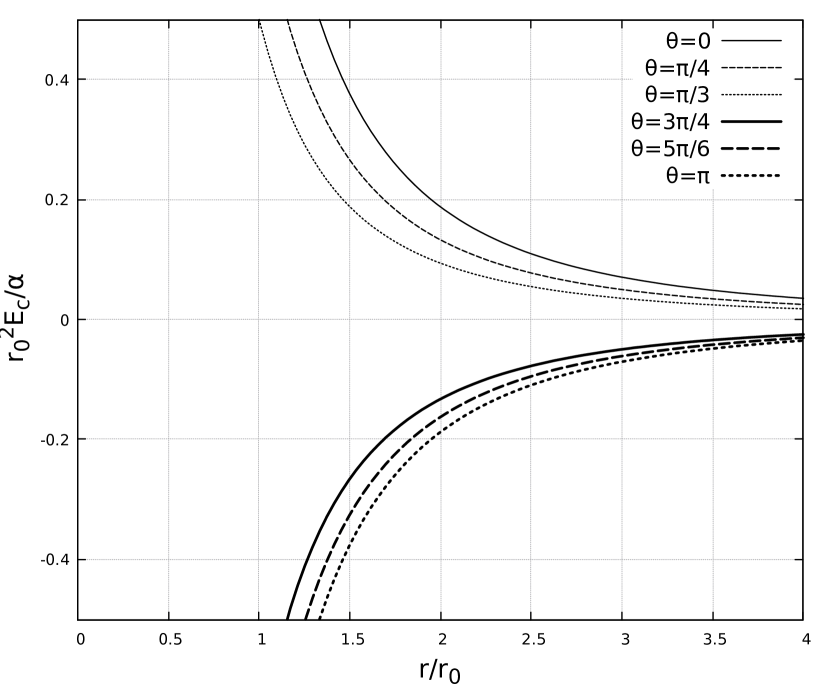
Figure 1: $\vec{E}_{c}\cdot\hat{\phi}\equiv E_{c}$, Eq. (72), as a function of $r/r_{0}$, for $\alpha=1/2$ for different angles $\theta$.

Figure 2: $\vec{B}_{c}\cdot\hat{r}\equiv B_{c,r}$, Eq. (73), as a function of $r/r_{0}$, for $\alpha=1/2$ and different angles $\theta$.

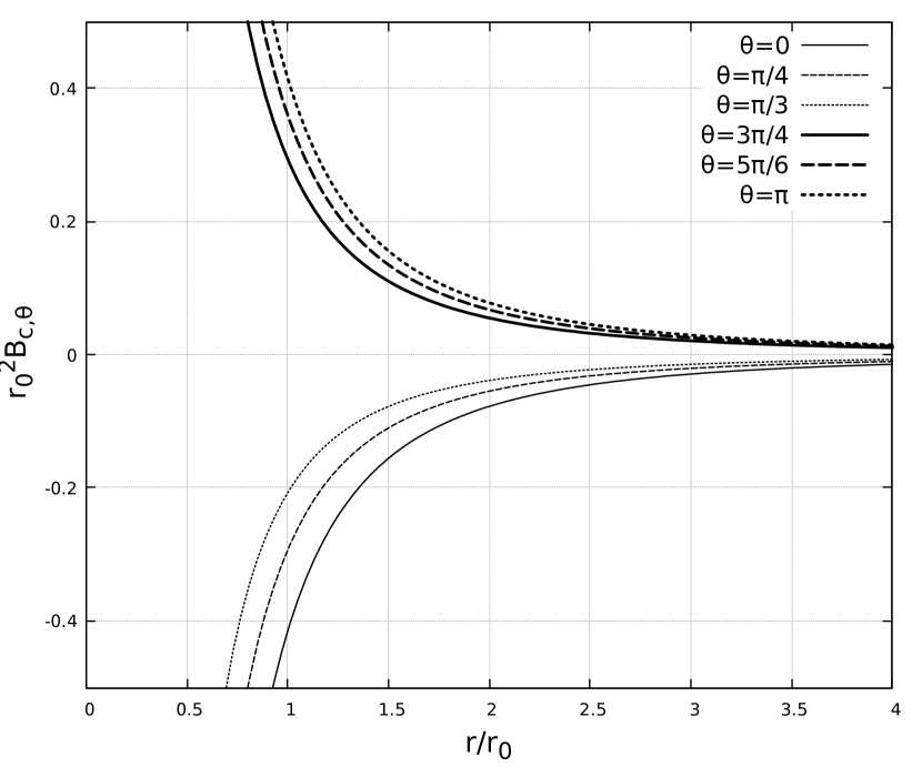
Figure 3: $\vec{B}_{c}\cdot\hat{\theta}\equiv B_{c,\theta}$, Eq. (73), as a function of $r/r_{0}$, for $\alpha=1/2$ and different angles $\theta$.

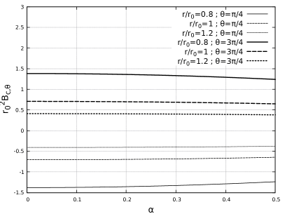
Figure 4: $\vec{B}_{c}\cdot\hat{\theta}\equiv B_{c,\theta}$, Eq. (73), as a function of $\alpha$ for different radial coordinates $r$ for different angles $\theta$.

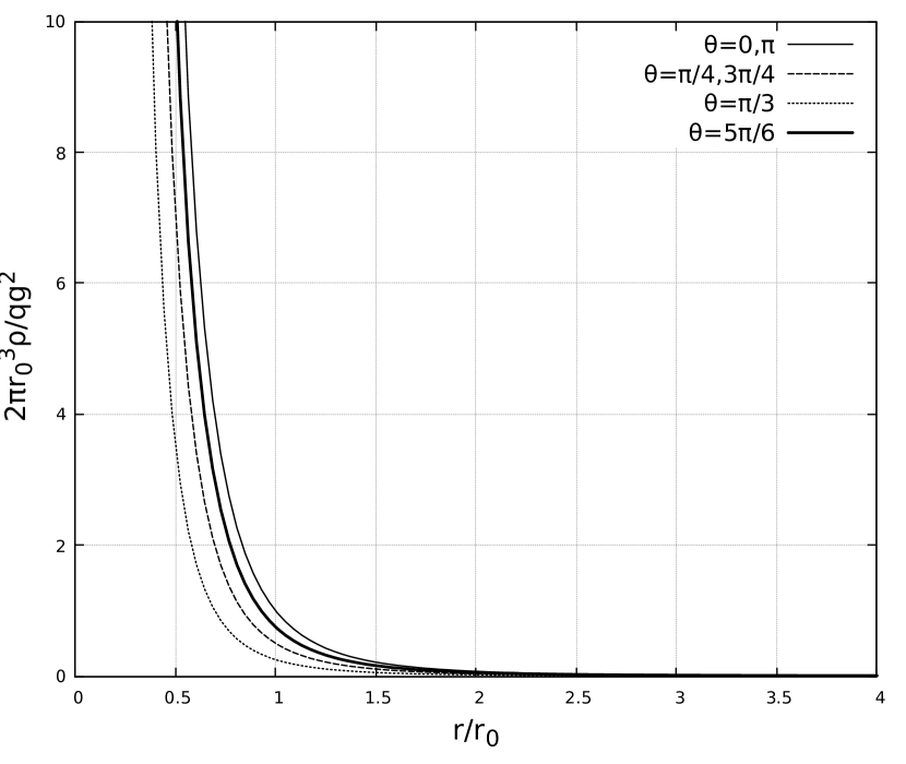
Figure 5: $\rho(r)$ as a function of $r/r_{0}$, Eq. (78), for $\alpha=1/2$ and different angles $\theta$.

The non-Abelian contribution to the energy density, ($u_{Ec,Bc}$), from Eq. B.11, is given by:

$$u_{Ec,Bc}(\alpha)= \frac{1}{2}\left(\frac{\cos^{2}(2\theta)}{\sin^{2}(\theta)}+\cos^{2}(\theta)\left(\frac{5}{2}-\sqrt{9-4\alpha^{2}}\right)\right)\frac{1}{r_{0}^{4}}\left(\frac{r_{0}}{r}\right)^{3+\sqrt{9-4\alpha^{2}}}.$$ (80)

The total energy will have a divergence that would need a short distance cutoff, similarly to the classical electron radius problem. However, besides an (expected) divergence of the charge in the origin $1/r^{(3+\sqrt{9-4\alpha^{2}})}$, analytical cuts appear in the angular extrema directions, $\theta=0,\pi$.

5 Anisotropic Coulomb potential: class of solutions

Before investigating other different well known solutions for the scalar potential, now, by using the ansatz 50, let us consider an anisotropic modification of the Coulomb potential by means of the following prescription:

$$\varphi(r,\theta)=\frac{f(\theta)}{r}.$$ (81)

As a source we consider a punctual charge in the origin and keep an additional arbitrary color-charge density $\rho(\vec{r})$ to be determined later. By considering more general equations, Eqs. (19)-(22), than those of the previous section, for an anisotropic potential we obtain the following equations:

$$\frac{1}{r}\nabla^{2}f(\theta)-4\pi\delta(\vec{r})f(\theta)-2g^{2}A_{\phi}^{2}\frac{f(\theta)}{r} =-\rho;$$ (82)

$$R_{\theta} =0;$$ (83)

$$r^{2}R_{\phi}^{\prime\prime}+2rR_{\phi}^{\prime}-l(l+1)R_{\phi} =0;$$ (84)

$$(1-x^{2})\frac{d^{2}\Theta_{\phi}}{dx^{2}}-2x\frac{d\Theta_{\phi}}{dx}+\left(g^{2}f^{2}(\theta)-\frac{1}{1-x^{2}}+l(l+1)\right)\Theta_{\phi} =0.$$ (85)

Equation 84 is the Euler-Cauchy equation [45], with the following solutions:

$$R_{\phi}(r)=a_{l}r^{\frac{-1-\sqrt{1+4l(l+1)}}{2}}+b_{l}r^{\frac{-1+\sqrt{1+4l(l+1)}}{2}}.$$ (86)

The prescription 81 can be solved for different cases of angular dependency, given by $f(\theta)=f(\cos(\theta))=f(x)$. As an example, consider the case:

$$f(x)=\frac{\lambda}{4\pi\sqrt{1-x^{2}}},$$ (87)

where $\lambda$ is a parameter that carries color charge which initially might be a sort of punctual although the rotational symmetry breaking must be a non-Abelian effect. With this prescription, equation 85 becomes:

$$(1-x^{2})\frac{d^{2}\Theta_{\phi}}{dx^{2}}-2x\frac{d\Theta_{\phi}}{dx}+\left(l(l+1)-\frac{1-(\lambda g/4\pi)^{2}}{1-x^{2}}\right)\Theta_{\phi} =0,$$ (88)

which is the Legendre’s associated equation of order $\sqrt{1-(Cg)^{2}}$, being $C=\lambda/(4\pi)$, [45]. The solutions can be written as:

$$\Theta_{\phi}=c_{l}P_{l}^{\sqrt{1-(Cg)^{2}}}(\cos(\theta))+d_{l}Q_{l}^{\sqrt{1-(Cg)^{2}}}(\cos(\theta)).$$ (89)

In order for these solutions to be real for all $\cos(\theta)$, we must have an integer for the order of the function. The only possibility is therefore given by:

$$|Cg|=\left|\frac{\lambda g}{4\pi}\right|=1.$$ (90)

This condition provides a large value for $|\lambda g/(4\pi)|$ than the corresponding solution of the (spherically symmetric) Coulomb potential of the last section - in Eq. (67). By considering the largest value $gC=1$, and with a condition that $\vec{A}(r\rightarrow\infty)\to 0$ , the solution for the vector potential is:

$$\vec{A}(\vec{r})=\sum_{l=0}^{\infty}a_{l}r^{\frac{-1-\sqrt{1+4l(l+1)}}{2}}\left(c_{l}P_{l}(\cos(\theta))+d_{l}Q_{l}(\cos(\theta))\right)\hat{\phi}.$$ (91)

Since no boundary conditions will be applied to this type of problem, let us analyze the two different lowest energies cases of $l$.

5.1 $l=0$

For this case, $P_{0}=1$, so we only are left with a non-trivial case if $d_{0}\neq 0$. Therefore, the solution is then:

$$\vec{A}(\vec{r})=\frac{1}{r}\left[c_{0}+d_{0}Q_{0}(\cos(\theta))\right]\hat{\phi},\mbox{ }Q_{0}(x)=\frac{1}{2}\ln\left(\frac{1+x}{1-x}\right).$$ (92)

As we see, $c_{0}$ and $d_{0}$ are dimensionless constants. They also have to be functions of $g$, such that in the Abelian limit ($g\rightarrow 0$), we recover the solution $\vec{A}=0$:

$$\lim_{g\rightarrow 0}c_{0}(g)=\lambda,\;\;\;\;\;\lim_{g\rightarrow 0}d_{0}(g)=0.$$ (93)

The corresponding c-electric and c-magnetic fields are given by by considering Eq. (27):

I-spin:

$$\vec{E}_{a}(\vec{r}) =\frac{\lambda}{4\pi\sin(\theta)r^{2}}\left(\hat{r}+\frac{\hat{\theta}}{\sin(\theta)}\right)\delta_{a3}+\frac{1}{\sin(\theta)r}\left(c_{0}+\frac{d_{0}}{2}\ln\left(\frac{1+\cos(\theta)}{1-\cos(\theta)}\right)\right)\hat{\phi}(\delta_{a1}-\delta_{a2});$$ (94)

$$\vec{B}_{a}(\vec{r}) =\frac{\hat{r}}{r^{2}\sin(\theta)}\left(c_{0}\cos(\theta)+d_{0}\left(\frac{\cos(\theta)}{2}\ln\left(\frac{1+\cos(\theta)}{1-\cos(\theta)}\right)-1\right)\right)(\delta_{a1}+\delta_{a2});$$ (95)

V-spin:

$$\vec{E}_{a}(\vec{r}) =\frac{\lambda}{4\pi\sin(\theta)r^{2}}\left(\hat{r}+\frac{\hat{\theta}}{\sin(\theta)}\right)\left(\frac{\delta_{a3}+\sqrt{3}\delta_{a8}}{2}\right)+\frac{1}{\sin(\theta)r}\left(c_{0}+\frac{d_{0}}{2}\ln\left(\frac{1+\cos(\theta)}{1-\cos(\theta)}\right)\right)\hat{\phi}(\delta_{a4}-\delta_{a5});$$ (96)

$$\vec{B}_{a}(\vec{r}) =\frac{\hat{r}}{r^{2}\sin(\theta)}\left(c_{0}\cos(\theta)+d_{0}\left(\frac{\cos(\theta)}{2}\ln\left(\frac{1+\cos(\theta)}{1-\cos(\theta)}\right)-1\right)\right)(\delta_{a4}+\delta_{a5});$$

U-spin:

$$\vec{E}_{a}(\vec{r}) =\frac{\lambda}{4\pi\sin(\theta)r^{2}}\left(\hat{r}+\frac{\hat{\theta}}{\sin(\theta)}\right)\left(\delta_{a3}-\frac{\sqrt{3}}{3}\delta_{a8}\right)+\frac{1}{\sin(\theta)r}\left(c_{0}+\frac{d_{0}}{2}\ln\left(\frac{1+\cos(\theta)}{1-\cos(\theta)}\right)\right)\hat{\phi}(\delta_{a6}-\delta_{a7});$$ (97)

$$\vec{B}_{a}(\vec{r}) =\frac{\hat{r}}{r^{2}\sin(\theta)}\left(c_{0}\cos(\theta)+d_{0}\left(\frac{\cos(\theta)}{2}\ln\left(\frac{1+\cos(\theta)}{1-\cos(\theta)}\right)-1\right)\right)(\delta_{a6}+\delta_{a7}).$$

The above solutions for the $\hat{\phi}$-component of the electric field and the (radial) component of the magnetic field are shown in the next figures separately for the two components with $c_{0}$ or $d_{0}$. Some profiles of the $E^{\phi}_{c}$ for different angles (those that are non divergent) are shown for $d_{0}=0$ ($c_{0}=0$) in Fig. 7 ((7)). Although the Ec field decreases with $1/r$ the angular dependence is very strong. The $c_{0}$ component has an unique sign for all directions, whereas the $d_{0}$ changes sign for $3\pi/2>\theta>\pi/2$. The c-magnetic field profiles for different angles are shown in Figs. (9) and (9) respectively for $d_{0}=0$ and $c_{0}=0$. The strong anisotropic behavior is also noted being that the change of sign of $B_{c}$ is present for the components $d_{0}$ of the c-electric field, in spite of being very different. As a consequence, the c-electric and c-magnetic fields, and also their fluxes, are strongly anisotropic.

The charge density, responsible for these configurations, is given by:

$$\rho(\vec{r}) =\frac{\lambda}{\sin(\theta)}\delta(\vec{r})-\frac{\lambda}{4\pi r^{3}\sin^{3}(\theta)}+2g\operatorname{sign}(\lambda)\frac{1}{r^{3}}\frac{\left[c_{0}+d_{0}Q_{0}(\cos(\theta)\right]^{2}}{\sin(\theta)}.$$ (98)

Note that the usual punctual charge has an anisotropic form with cuts along $\theta=0,\pi$ which are responsible for the scalar potential (81), besides other extended contributions all of them with cuts in the same directions and the singularities in $r=0$.

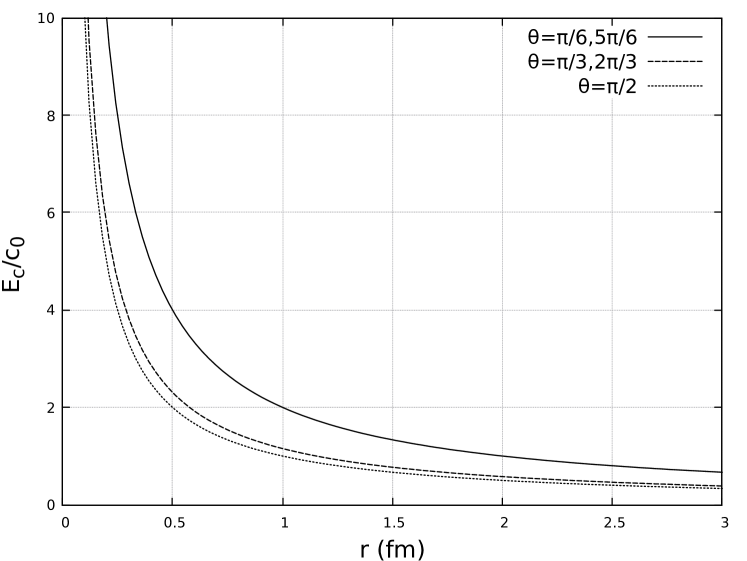
Figure 6: $E_{c}^{\phi}$, from 94, for $d_{0}=0$.

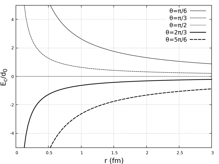
Figure 7: $E_{c}^{\phi}$, from 94, for $c_{0}=0$.

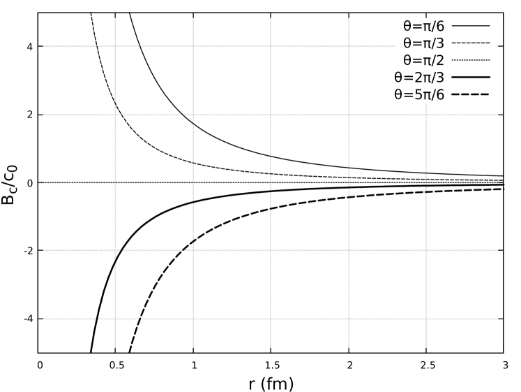
Figure 8: $B_{c}^{r}$, from 95, for $d_{0}=0$.

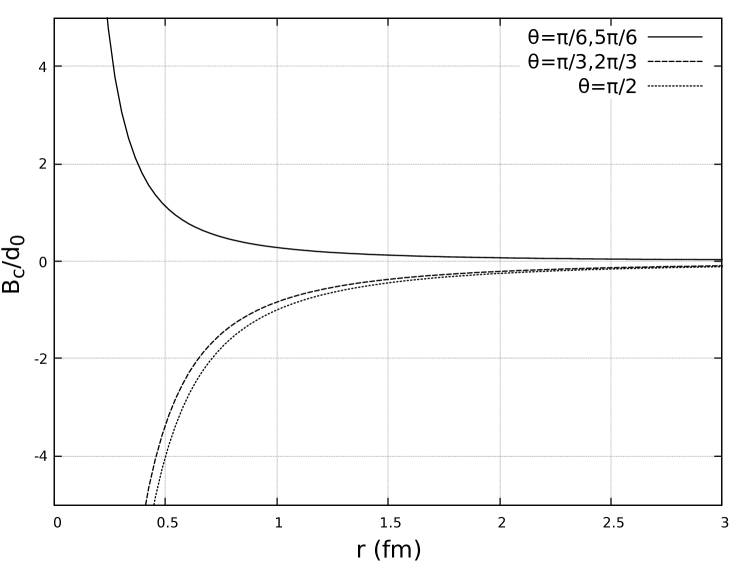
Figure 9: $B_{c}^{r}$, from 95, for $c_{0}=0$.

5.2 $l=1$

In this case the vector potential reads:

$$\vec{A}(\vec{r})=\frac{1}{r^{2}}\left(c_{1}P_{1}(\cos(\theta)+d_{1}Q_{1}(\cos(\theta))\right)\hat{\phi},\mbox{ }P_{1}(x)=x\mbox{ and }Q_{1}(x)=\frac{x}{2}\ln\left(\frac{1+x}{1-x}\right)-1.$$ (99)

As we expect $\vec{A}$ to vanish in the limit $g\rightarrow 0$, $d_{1}$ must be some function of $g$ such that this condition is obtained, so we rename:

$$c_{1} =\epsilon r_{0}(g);$$ (100)

$$d_{1} =\gamma r_{0}(g),$$ (101)

where $r_{0}(g)$ is a function of g such that $r_{0}(0)=0$, representing our new integration constant that satisfies the eletromagnetic limit, and $\gamma$, $\epsilon$ are fitting dimensioneless constants. Therefore:

$$\vec{A}(\vec{r})=\frac{1}{r_{0}}\left(\frac{r_{0}}{r}\right)^{2}\left(\gamma\cos(\theta)+\epsilon\left[\frac{\cos(\theta)}{2}\ln\left(\frac{1+\cos(\theta)}{1-\cos(\theta)}\right)-1\right]\right)\hat{\phi}.$$ (102)

The corresponding c-electric and c-magnetic fields for each of the SU(2) subgroups are given by (using 27):

I-spin:

$$\vec{E}_{a}(\vec{r}) =\frac{\lambda}{4\pi\sin(\theta)r^{2}}\left(\hat{r}+\frac{\hat{\theta}}{\sin(\theta)}\right)\delta_{a3}+\frac{\operatorname{sign}(\lambda)}{\sin(\theta)r_{0}^{2}}\left(\frac{r_{0}}{r}\right)^{3}\left(\gamma P_{1}(\cos(\theta)+\epsilon Q_{1}(\cos(\theta)\right)\hat{\phi}(\delta_{a1}-\delta_{a2});$$ (103)

$$\vec{B}_{a}(\vec{r}) =\frac{1}{r_{0}^{2}}\left(\frac{r_{0}}{r}\right)^{3}\left[\frac{\hat{r}}{\sin(\theta)}\left(\gamma\cos(2\theta)-\epsilon\left(Q_{0}(\cos(\theta)+\frac{\cos(\theta)}{2}\right)\right)+\hat{\phi}\left(\gamma P_{1}(\cos(\theta)+\epsilon Q_{1}(\cos(\theta)\right)\right](\delta_{a1}+\delta_{a2});$$ (104)

V-spin:

$$\vec{E}_{a}(\vec{r}) =\frac{\lambda}{4\pi\sin(\theta)r^{2}}\left(\hat{r}+\frac{\hat{\theta}}{\sin(\theta)}\right)\left(\frac{\delta_{a3}+\sqrt{3}\delta_{a8}}{2}\right)+\frac{\operatorname{sign}(\lambda)}{\sin(\theta)r_{0}^{2}}\left(\frac{r_{0}}{r}\right)^{3}\left(\gamma P_{1}(\cos(\theta)+\epsilon Q_{1}(\cos(\theta)\right)\hat{\phi}(\delta_{a4}-\delta_{a5});$$

$$\vec{B}_{a}(\vec{r}) =\frac{1}{r_{0}^{2}}\left(\frac{r_{0}}{r}\right)^{3}\left[\frac{\hat{r}}{\sin(\theta)}\left(\gamma\cos(2\theta)-\epsilon\left(Q_{0}(\cos(\theta)+\frac{\cos(\theta)}{2}\right)\right)+\hat{\phi}\left(\gamma P_{1}(\cos(\theta)+\epsilon Q_{1}(\cos(\theta)\right)\right](\delta_{a4}+\delta_{a5});$$

U-spin:

$$\vec{E}_{a}(\vec{r}) =\frac{\lambda}{4\pi\sin(\theta)r^{2}}\left(\hat{r}+\frac{\hat{\theta}}{\sin(\theta)}\right)\left(\delta_{a3}-\frac{\sqrt{3}}{3}\delta_{a8}\right)+\frac{\operatorname{sign}(\lambda)}{\sin(\theta)r_{0}^{2}}\left(\frac{r_{0}}{r}\right)^{3}\left(\gamma P_{1}(\cos(\theta)+\epsilon Q_{1}(\cos(\theta)\right)\hat{\phi}(\delta_{a6}-\delta_{a7});$$

$$\vec{B}_{a}(\vec{r}) =\frac{1}{r_{0}^{2}}\left(\frac{r_{0}}{r}\right)^{3}\left[\frac{\hat{r}}{\sin(\theta)}\left(\gamma\cos(2\theta)-\epsilon\left(Q_{0}(\cos(\theta)+\frac{\cos(\theta)}{2}\right)\right)+\hat{\phi}\left(\gamma P_{1}(\cos(\theta)+\epsilon Q_{1}(\cos(\theta)\right)\right](\delta_{a6}+\delta_{a7}),$$

where we have used the relation 90. The corresponding charge density for all subgroups is given by:

$$\rho(\vec{r}) =\frac{\lambda}{\sin(\theta)}\delta(\vec{r})-\frac{\lambda}{4\pi r^{3}\sin^{3}(\theta)}+\frac{2g\operatorname{sign}(\lambda)}{r^{3}_{0}\sin(\theta)}\left(\frac{r_{0}}{r}\right)^{4}\left(\gamma P_{1}(\cos(\theta)+\epsilon Q_{1}(\cos(\theta))\right)^{2}.$$ (105)

It presents a strong anisotropy that is a non-Abelian effect from the vector potential. Similarly to the case of $l=0$ (and also to the magnetic field of the previous spherically symmetric Coulomb potential) the presence of the terms with $1/(\sin^{n}\theta)$ - odd n - may be an indication of a dipolar type configuration with the unusual presence of analytical cuts for $\theta=0,2\pi$. Similarly to other situations addressed in the present work, this color-charge density could be associated to a classical gluon cloud around a punctual quark in the origin similarly to the solution of the previous section for a spherical symmetric Coloumb potential (4).

In Figs. (11) and (11) the (normalized, dimensionless) strength of the component $E_{\phi}$ of the c-electric field are shown respectively for $\gamma=0$ and $\epsilon=0$ in Eq. (103) for different angles $\theta$. For $\theta=0,\pi$ the Ec component is singular. This non-Abelian component of the Ec field has a singularity of $1/r^{3}$. Similarly to the case of $l=0$ there is a component of the c-electric field that does not change sign and another that changes sign depending on the octant they are placed. Similarly the radial and angular (normalized and dimensionless) components of $B_{c}$, $B_{c,r}$ and $B_{c,\theta}$, are shown separately for components with $\gamma$ and $\epsilon$ in Figs. (13,13) - for $B_{c,r}$ - and Figs. (15,15) - for $B_{c,\phi}$ - for some angles $\theta$. They have similar behavior as the Ec field, with singularities for $\theta=0,\pi$, except that they are zero for different angles. These color-electric and magnetic fields have a similar shape as the fields to the (1) lower component $l=0$ shown in section (5.1) and to the (2) spherical symmetric Coulomb potential of the previous section, as it can be seen in Figs. (1,3) and (3) although the specific angular dependencies are different.

Figure 10: $\vec{E}_{c}\cdot\hat{\phi}$, Eq. (103), as a function of $r/r_{0}$ for different $\theta$, and $\gamma=0$.

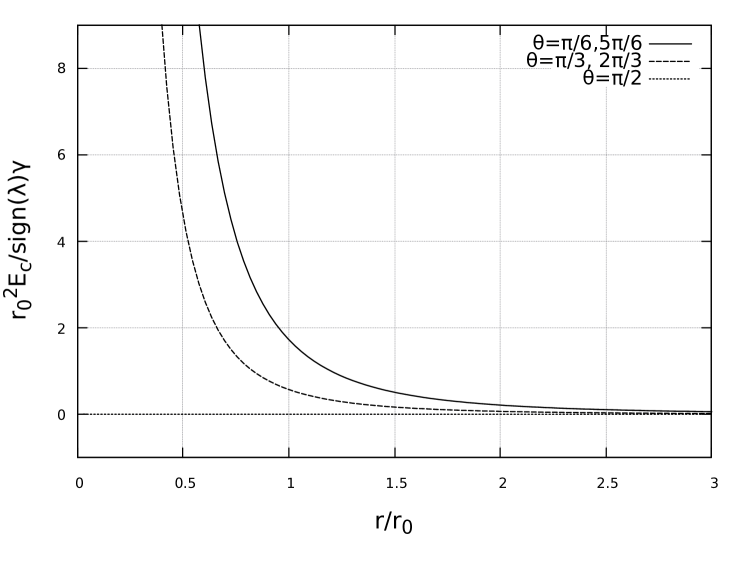
Figure 11: $\vec{E}_{c}\cdot\hat{r}=E_{c,r}$, Eq. (103) as a function of $r/r_{0}$ for different $\theta$, and $\epsilon=0$.

-

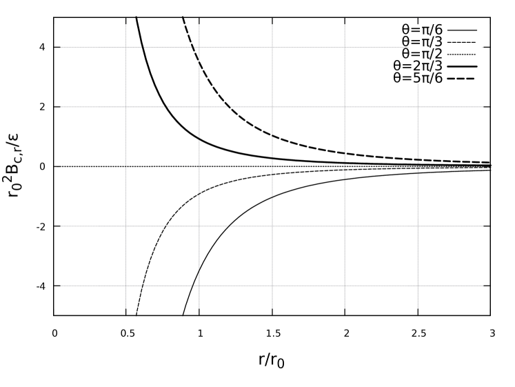
Figure 12: $\vec{B}_{c}\cdot\hat{r}\equiv B_{c,r}$, equation 104, as a function of $r/r_{0}$ for different $\theta$, and $\gamma=0$.

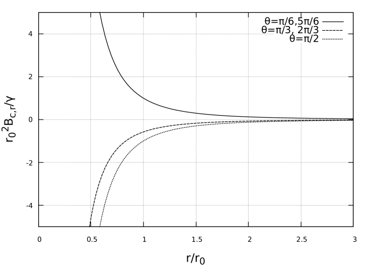
Figure 13: $\vec{B}_{c}\cdot\hat{r}\equiv B_{c,r}$, equation 104, as a function of $r/r_{0}$ for different $\theta$, and $\epsilon=0$.

-

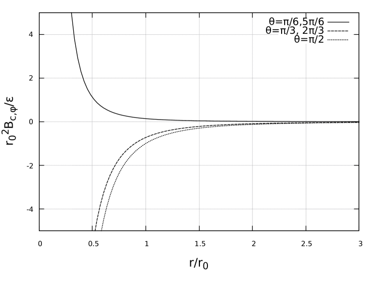
Figure 14: $\vec{B}_{c}\cdot\hat{\phi}\equiv B_{c,\phi}$, equation 104, as a function of $r/r_{0}$ for different $\theta$, and $\gamma=0$.

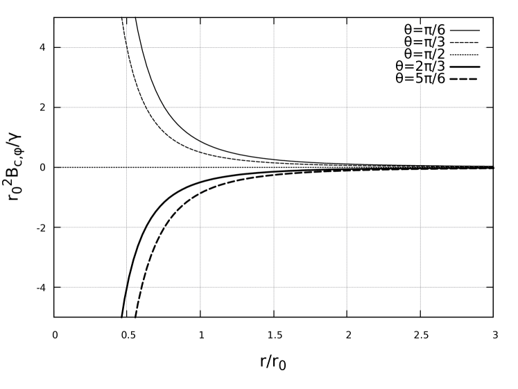
Figure 15: $\vec{B}_{c}\cdot\hat{\phi}\equiv B_{c,\phi}$, equation 104, as a function of $r/r_{0}$ for different $\theta$, and $\epsilon=0$.

The color-charge density, Eq. (105), is shown in Fig. (16) for the same angles considered for the previous figures. Again the change of sign of the color-charge density occurs for a particular angle $\theta$ whose determination is not trivial for the case of $l=1$. This configuration corresponds to a somewhat dipole type color-charge distribution for which, however, a cutoff in the angle $\theta\neq 0,\pi$ is required to avoid the analytical cuts. It is interesting to note that the curves that are positive for small $r$ ($\pi/6$ and $\pi/3$) cross the horizontal axis in the points in which $\rho(\vec{r})=0$ according to Eq. (105). These points of zero color charge do not define a closed surface containing the origin (where the color charge responsible for the (modified) Coulomb potential lies) because of the analytical cuts.

Figure 16: Charge density, equation 105, as a function of $r/r_{0}$ for different $\theta$, with $g=1$ and $\gamma=\epsilon=1$.

6 Linear potential

In this section, we’ll impose the scalar potential to be given by a linearly rising potential without imposing a charge distribution from the beginning. Therefore we go back to the Eqs. (53-55). Consider the scalar potential to be given by:

$$\varphi(\vec{r})=\kappa r,$$ (106)

where $\kappa$ is a constant that carries the color charge from Eq. (28). The unknown quark density $\rho(\vec{r})$ will be considered to be the one that makes eq. (106) a solution of the eq. (53). The vector potential will be considered to have only the angular components. Eq. 53 can be seen therefore as a constraint, in which case reads:

$$\rho(\vec{r})=2g^{2}\left(A_{\theta}^{2}(\vec{r})+A_{\phi}^{2}(\vec{r})\right)\kappa r-\frac{2\kappa}{r},\;\;\;\;\;\mbox{ for }\;\;r\leq R_{max},$$ (107)

that might be seen as a constraint for the angular components of the vector potential. Also, we notice that in order for $\rho$ to be naturally contained in some region, the vector potential must go to zero faster than the linear potential increases as $r\rightarrow\infty$. Otherwise, an external boundary may be imposed, maybe by quantum fluctuations. In any case, the decreasing part, $2\kappa/r$, must be confined in a region for which a closed wall such as a sphere can be imposed. As a consequence, all the solutions will be valid inside such a closed region in which there is an extended color-charge distribution.

From 54 and the prescription for the linear $\varphi$ potential, we may obtain a solution by re-scaling $R_{\theta}$ by:

$$R_{\theta}(r)=\frac{e^{-i\frac{g\kappa}{2}r^{2}}M\left(\sqrt{ig\kappa}r\equiv x\right)}{r},$$ (108)

where the resulting equation for $M(x=\sqrt{ig\kappa r})$ is the following:

$$\frac{d^{2}M}{dx^{2}}-2x\frac{dM}{dx}-M=0,$$ (109)

wich has the solutions:

$$M=aH_{-1/2}(x)+be^{x^{2}/2}\sqrt{x}I_{-1/4}\left(\frac{x^{2}}{2}\right),$$ (110)

where $H_{\alpha}(x)$ and $I_{\alpha}(x)$ are the generalized Hermite and Bessel (1st kind) functions, respectively. Then:

$$R_{\theta}=\frac{e^{-i\frac{g\kappa}{2}r^{2}}}{r}\left(aH_{-1/2}(\sqrt{ig\kappa}r)+be^{x^{2}/2}\sqrt{x}I_{-1/4}\left(\frac{ig\kappa r^{2}}{2}\right)\right).$$ (111)

For the phi-component, that is separable, it can be written:

$$A_{\phi}(\vec{r})=R_{\phi}(r)\Theta_{\phi}(\theta),$$ (112)

and the following equations ($x\equiv\cos(\theta)$) are obtained:

$$r^{2}\frac{d^{2}R_{\phi}}{dr^{2}}+2r\frac{dR_{\phi}}{dr}+\left((g\kappa)^{2}r^{4}-l(l+1)\right)R_{\phi} =0;$$ (113)

$$(1-x^{2})\frac{d^{2}\Theta_{\phi}}{dx^{2}}-2x\frac{d\Theta_{\phi}}{dx}+\left(l(l+1)-\frac{1}{1-x^{2}}\right)\Theta_{\phi} =0.$$ (114)

The equation for $\Theta_{\phi}$ is the Legendre associated equation of degree $l$ and order $\pm 1$ [45]. The equation for $R_{\phi}$ is solved by the re-scaling:

$$R_{\phi}(r)=\frac{S\left(\frac{g\kappa r^{2}}{2}\equiv v\right)}{\sqrt{r}}.$$ (115)

This change of variable leads to a Bessel’s equation [45], whose solution can be written as:

$$R_{\phi}(r)=\frac{c_{l}J_{\frac{2l+1}{2}}\left(\frac{g\kappa r^{2}}{2}\right)+d_{l}Y_{\frac{2l+1}{2}}\left(\frac{g\kappa r^{2}}{2}\right)}{\sqrt{r}}.$$ (116)

Then, the complete solution for the vector potential is:

$$\vec{A}(\vec{r})=\frac{e^{-i\frac{g\kappa}{2}r^{2}}}{r\sin(\theta)}\left(aH_{-1/2}(\sqrt{ig\kappa}r)+be^{x^{2}/2}\sqrt{x}I_{-1/4}\left(\frac{ig\kappa r^{2}}{2}\right)\right)\hat{\theta}+\sum_{l=1}^{\infty}\frac{c_{l}J_{l+\frac{1}{2}}\left(\frac{g\kappa r^{2}}{2}\right)+d_{l}Y_{l+\frac{1}{2}}\left(\frac{g\kappa r^{2}}{2}\right)}{\sqrt{r}}P^{1}_{l}(\cos(\theta))\hat{\phi}.$$ (117)

Now, by requiring only real-valued functions such that $\vec{A}$ is real, it follows that $a=b=0$. Consider now the simplest case, $l=1$, for which it can be written:

$$\vec{A}(\vec{r})=-\frac{c_{1}J_{3/2}\left(\frac{g\kappa r^{2}}{2}\right)+d_{1}Y_{3/2}\left(\frac{g\kappa r^{2}}{2}\right)}{\sqrt{r}}\sin(\theta)\hat{\phi},$$ (118)

where:

$$J_{3/2}(x) =\sum_{k=0}^{\infty}\frac{(-1)^{k}(x/2)^{2k+3/2}}{k!\Gamma(k+5/2)},$$ (119)

$$Y_{3/2}(x) =\sum_{k=0}^{\infty}\frac{(-1)^{k}(x/2)^{2k-3/2}}{k!\Gamma(k-1/2)}.$$ (120)

Note that $R_{\theta}$ has a dimensionless constant of integration and $R_{\phi}$ has its constant with dimension length${}^{-\frac{1}{2}}$.

Consider the case where the singularities at the origin in the vector potential is limited to the $1/\sqrt{r}$ that appears dividing the $J$ and $Y$ in Eq. (118)., and $d_{1}=0$. By re-defining the constant the $c_{1}$ as:

$$c_{1} =\operatorname{sign}(c_{1})\frac{1}{\sqrt{r_{1}}},$$ (121)

where:

$$\operatorname{sign}(x)=\begin{cases}+1,\mbox{ if }x>0,\\ -1,\mbox{ if }x<0,\end{cases}$$ (122)

the solution becomes:

$$\vec{A}(\vec{r})=-\operatorname{sign}(c_{1})\sqrt{\frac{r_{1}}{r}}J_{3/2}\left(\frac{g\kappa r^{2}}{2}\right)\frac{\sin(\theta)}{r_{1}}\hat{\phi}.$$ (123)

With this, the charge density, C-Electric and C-Magnetic fields for each of the SU(2) subgroups with the condition 27) are, respectively:

I-spin:

$$\vec{E}_{a}(\vec{r}) =\kappa\hat{r}\delta_{a3}-g\kappa\operatorname{sign}(c_{1})\sqrt{\frac{r}{r_{1}}}J_{3/2}\left(\frac{g\kappa r^{2}}{2}\right)\sin(\theta)\hat{\phi}(\delta_{a1}-\delta_{a2});$$ (124)

$$\vec{B}_{a}(\vec{r}) =-\operatorname{sign}(c_{1})\frac{1}{r_{1}^{2}}\left[\hat{r}\left(\frac{r_{1}}{r}\right)^{3/2}2J_{3/2}\left(\frac{g\kappa r^{2}}{2}\right)\cos(\theta)\right.$$

$$\left.-\hat{\theta}\sin(\theta)\left(\left(\frac{r_{1}}{r}\right)^{3/2}2J_{3/2}\left(\frac{g\kappa r^{2}}{2}\right)-g\kappa r_{1}^{2}J_{5/2}\left(\frac{g\kappa r^{2}}{2}\right)\right)\right](\delta_{a1}+\delta_{a2});$$ (125)

V-spin:

$$\vec{E}_{a}(\vec{r}) =\kappa\hat{r}\left(\frac{1}{2}\delta_{a3}+\frac{\sqrt{3}}{2}\delta_{a8}\right)-g\kappa\operatorname{sign}(c_{1})\sqrt{\frac{r}{r_{1}}}J_{3/2}\left(\frac{g\kappa r^{2}}{2}\right)\sin(\theta)\hat{\phi}(\delta_{a4}-\delta_{a5});$$ (126)

$$\vec{B}_{a}(\vec{r}) =-\operatorname{sign}(c_{1})\frac{1}{r_{1}^{2}}\left[\hat{r}\left(\frac{r_{1}}{r}\right)^{3/2}2J_{3/2}\left(\frac{g\kappa r^{2}}{2}\right)\cos(\theta)\right.$$

$$\left.-\hat{\theta}\sin(\theta)\left(\left(\frac{r_{1}}{r}\right)^{3/2}2J_{3/2}\left(\frac{g\kappa r^{2}}{2}\right)-g\kappa r_{1}^{2}J_{5/2}\left(\frac{g\kappa r^{2}}{2}\right)\right)\right](\delta_{a4}+\delta_{a5});$$ (127)

U-spin:

$$\vec{E}_{a}(\vec{r}) =\kappa\hat{r}\left(\delta_{a3}-\frac{\sqrt{3}}{3}\delta_{a8}\right)-g\kappa\operatorname{sign}(c_{1})\sqrt{\frac{r}{r_{1}}}J_{3/2}\left(\frac{g\kappa r^{2}}{2}\right)\sin(\theta)\hat{\phi}(\delta_{a6}-\delta_{a7});$$ (128)

$$\vec{B}_{a}(\vec{r}) =-\operatorname{sign}(c_{1})\frac{1}{r_{1}^{2}}\left[\hat{r}\left(\frac{r_{1}}{r}\right)^{3/2}2J_{3/2}\left(\frac{g\kappa r^{2}}{2}\right)\cos(\theta)\right.$$

$$\left.-\hat{\theta}\sin(\theta)\left(\left(\frac{r_{1}}{r}\right)^{3/2}2J_{3/2}\left(\frac{g\kappa r^{2}}{2}\right)-g\kappa r_{1}^{2}J_{5/2}\left(\frac{g\kappa r^{2}}{2}\right)\right)\right](\delta_{a6}+\delta_{a7}),$$ (129)

The corresponding charge density will be given by:

$$\rho(\vec{r}) =\frac{\kappa}{r_{1}}\left(2g^{2}\sin^{2}(\theta)\left[J_{3/2}\left(\gamma\left(\frac{r}{r_{1}}\right)^{2}\right)\right]^{2}-2\frac{r_{1}}{r}\right).$$ (130)

This color-charge density is shown in Fig. (18) for different angles as a function of the (normalized) radial coordinate $r/r_{1}$ for $\gamma=0.1$ and $g=1$. Note that for a small solid angle around $\pi/2$ the color charge density reaches zero(s) for quite shorter distances as compared to its possible reaching distances. These values were also adopted for the next Figs. (18),(20) and (20) for the c-electric and c-magnetic fields. For larger values of $\gamma$, the c-electric and the c-magnetic fields oscillate progressively more at short distances, so that for smaller values of $\gamma$ the oscillations still happens although they take place for larger $r/r_{1}$. The strongly anisotropic behavior is present in the chromo-electric and chromo-magnetic fields that are shown in Figs. (18,20) and (20) for different angles $\theta$. The field $E_{c}$ and the component $B_{c,r}$ have their zeros at the same point and the component $B_{c,\theta}$ has zero in smaller values of $r/r_{1}$. Only the radial component $B_{c,r}$ changes sign for specific directions, specifically for $-\pi/2<\theta<\pi/2$. Note that, again the Ec and Bc fluxes are highly anisotropic, similarly to the effects discussed above for the strict Coulomb potential.

The parameter $r_{1}=1/c_{1}^{2}$ is related to the normalization of gauge vector potential, $\vec{A}\cdot\hat{\phi}$, that, together with the dimensionless parameter $\gamma=gr^{2}\kappa/2$, settle possible zeros for the color-charge density $\rho(r,\theta)$, that is highly anisotropic. Analogously to the case of anisotropic Coulomb potential a surface of zero color-charge density can also be defined by:

$$\frac{r_{1}}{r}=g^{2}\sin^{2}(\theta)\left[J_{3/2}\left(\gamma\left(\frac{r}{r_{1}}\right)^{2}\right)\right]^{2}.$$ (131)

It can be seen, however, that for $\theta=0,\pi$, there are no zeros of the color-charge density. The non-Abelian contribution is intrinsically non-spherically symmetric. Therefore, the shape of the relation 131 gives us information about the shape of the localized charge distribution although it is not limited to a closed region in space. The color charge density might also change its sign as one increases the radial coordinate $r$ and in this case, a total zero color charge might be found for an extended color distribution. In some sense, this is remarkably similar to a bag model for a "non-spheric bag" and possibly, a different mechanism or external restriction of its spatial distribution should be imposed. These solutions are more well behaved than the solutions found for the extension of the Coulomb potential of Sec. (5). We did not find a straightforward way to fix the constant $\kappa$, as it would be desirable, although this is possible in a precarious way for a particular value of $\gamma$ and a particular radius $r=R_{0}$ the following definition appeared above:

$$\kappa=\frac{2\gamma_{0}}{gR_{0}^{2}}$$ (132)

where $\gamma_{0}=\gamma(R_{0}^{2}/r_{1}^{2})$. The linear potential found in lattice QCD is rather expected to be leading at larger distances in comparison to the shorter distances in which the Coulomb potential, and others must be more important. In the specific radial coordinate $R_{0}$ is related to the characteristic distance $r_{1}$ above, it is associated to the vector potential normalization from Eq. (121). For $\gamma=0.1$ the color-charge density reaches zero, $\rho(\vec{r})=0$, for a solid angle around $\theta=\pi/2$ for $R_{0}/r_{1}\sim 4$ from Fig. (18). By adopting $R_{0}/r_{1}=x$, and the same normalization for both the scalar and vector potentials $|\frac{1}{r_{1}}|\sim|\kappa R_{0}|$, one has: $\kappa=g/(2x^{4}\gamma^{2}R_{0}^{2})$. By considering $x\sim 4$, $g\simeq 1$, $R_{0}\sim 0.5$ fm. and $\gamma\sim 0.1$ it yields $\kappa\sim 0.03$ GeV² that is somewhat smaller than $\sigma_{latt}\sim 0.19$ GeV² [2, 10]. The total color-charge contained in a sphere of radius $R$ as a function of the normalized radius $R/r_{1}$ is presented in Fig. (21).

Figure 17: The (normalized and dimensionless) color-charge distribution $\rho(r)$, Eq. (130 as a function of $r/r_{1}$, for $g=1$ for $\gamma=0.1$.

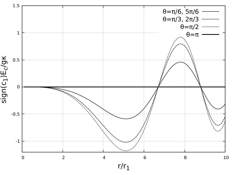
Figure 18: The normalized and dimensionless $E_{c}$, Eq. (124), as a function of $r/r_{1}$ for $\gamma=0.1$.

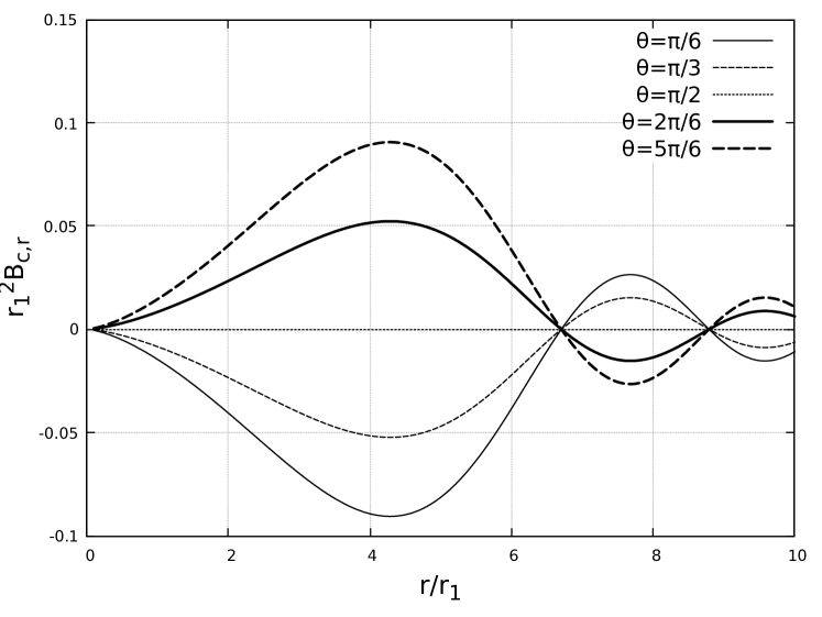
Figure 19: The normalized and dimensionless $\vec{B}_{c}\cdot\hat{r}\equiv B_{c,r}$, Eq. (125), as a function of $r/r_{1}$ for $\gamma=0.1$.

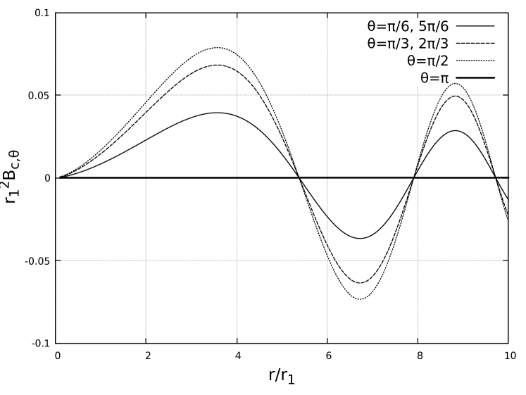
Figure 20: The normalized and dimensionless $\vec{B}_{c}\cdot\hat{\theta}\equiv B_{c,\theta}$, Eq. (125), as a function of $r/r_{1}$ for $\gamma=0.1$.

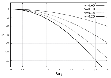
Figure 21: Total color-charge contained in a sphere of radius $R$ as a function of $R/r_{1}$, for different values of $\gamma$.

7 Yukawa potential

In this section the following spherical symmetric Yukawa type potential will be considered:

$$\varphi(\vec{r})=-C\frac{e^{-\frac{r}{r_{0}}}}{r},$$ (133)

where $r_{0}$ is a parameter to be determined. The equations 53 - 55 can be solved by separation of variables ($A_{\phi}(\vec{r})=R_{\phi}(r)\Theta_{\phi}(\cos(\theta)\equiv x)$) whose resulting equations can be written as:

$$r^{2}\frac{d^{2}R_{\theta}}{dr^{2}}+2r\frac{dR_{\theta}}{dr}+(gC)^{2}e^{-2r/r_{0}}R_{\theta} =0,$$ (134)

$$r^{2}\frac{d^{2}R_{\phi}}{dr^{2}}+2r\frac{dR_{\phi}}{dr}+\left((gC)^{2}e^{-2r/r_{0}}-l(l+1)\right)R_{\phi} =0,$$ (135)

$$(1-x^{2})\frac{d^{2}\Theta_{\phi}}{dx^{2}}-2x\frac{d\Theta_{\phi}}{dx}+\left(l(l+1)-\frac{1}{1-x^{2}}\right)\Theta_{\phi} =0.$$ (136)

Equations (134) and (135) do not depend on the normalization of $R_{\theta}$ and $R_{\phi}$ and therefore the more general solution may be obtained by multiplied them by a constant $a$, i.e $aR_{\theta}$ and $aR_{\phi}$ that will be searched numerically. Again, the solution for the angular part, equation (136), is given by Legendre’s associated functions of order $\pm 1$. It’s interesting to see that the equation for $R_{\theta}$ is a particular case of the one for $R_{\phi}$, namely, $l=0$. The resulting color-charge density that yield the solutions above is given by

$$\rho(\vec{r})=\frac{Ce^{-\frac{r}{r_{0}}}}{r}\left(\frac{1}{r_{0}^{2}}-2g^{2}A^{2}(\vec{r})\right).$$ (137)

To total charge $Q$ given by integration of 137 diverges if the functions $R_{\phi},R_{\theta},\Theta_{\theta}$ are given by the associated Legendre’s functions of the second kind. Therefore, if we impose that the only acceptable solutions are given by the $P^{m}_{l}(\cos(\theta))$ (implying that $R_{\theta}=0$), we have:

$$Q=4\pi C\left(1-g^{2}\frac{2(l+m)!}{(2l+1)(l-m)!}\int_{0}^{\infty}e^{-r/r_{0}}r(R_{\phi})^{2}dr\right)$$ (138)

The equation for $\Theta_{\phi}$, 136, can be solved for $x$, arriving at:

$$\Theta_{\phi}(\theta)=c\cosh\left(\ln\sqrt{\frac{1-x}{1+x}}\right)+b\sinh\left(\ln\sqrt{\frac{1-x}{1+x}}\right),$$ (139)

where $c$ and $b$ are the integration constants. Then, the full solution for $\vec{A}$ is given by:

$$\vec{A}(\vec{r})=\frac{R_{\theta}(r)}{\sin(\theta)}\hat{\theta}+R_{\phi}(r)\left(c\cosh\left(\ln\sqrt{\frac{1-\cos(\theta)}{1+\cos(\theta)}}\right)+b\sinh\left(\ln\sqrt{\frac{1-\cos(\theta)}{1+\cos(\theta)}}\right)\right)\hat{\phi},$$ (140)

where the normalization of each of the components are implicit and they are obtained numerically.

Analytical solutions for $R_{\theta}$ and $R_{\phi}$ have not been found, and numerical solutions were searched for the following boundary conditions:

$$\mbox{{BC1:}}\;\;\;\lim_{r=\delta r\rightarrow 0}R_{\theta,\phi} \sim-\frac{1}{\delta r}\to-\infty;$$

$$\lim_{r=\delta r\rightarrow 0}\frac{dR_{\theta,\phi}}{dr} \sim\frac{1}{(\delta r)^{2}}\to\infty,$$ (141)

and:

$$\mbox{{BC2:}}\;\;\;\lim_{r\rightarrow 0}R_{\theta,\phi} \sim\frac{1}{\delta r}\to\infty;$$

$$\lim_{r\rightarrow 0}\frac{dR_{\theta,\phi}}{dr} \sim-\frac{1}{(\delta r)^{2}}\to-\infty.$$ (142)

The resulting profiles for the lowest $l\geq 1$ exhibit somewhat unphysical oscillatory or divergent behavior that are not exhibited. So, below we show solutions for $l=0$ in which case we have the same equations for $R_{\theta}$ and $R_{\phi}$.

In Fig. (23), solutions for the normalized/dimensionless $CR=CR_{\theta},R_{\phi}$ with $l=0$ for the boundary conditions at the origin given by (7) are shown. By increasing the value of $gC$ the asymptotic value $R(r\to\infty)$ becomes more negative. In Fig. (23), solutions for $CR=CR_{\theta},R_{\phi}$ with $l=0$ for the boundary conditions at the origin given by (7) are shown. By increasing the value of $gC$ the asymptotic value $R(r\to\infty)$ becomes more positive. In both cases, however, for $(gC)^{2}\approx 2.33$ (i.e. $gC\simeq 1.53$) the asymptotic values go to zero $R(r\to\infty)=0$.

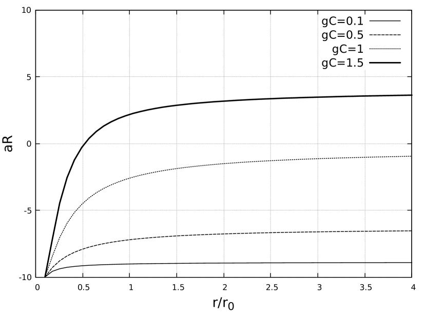
Figure 22: Numerical solutions for Eq. (135) for the boundary condition at the origin (7) and for different values of $gC$, and the integration constant $a$ made explicit.

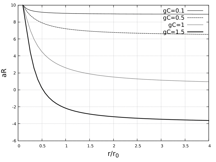
Figure 23: Numerical solutions for Eq. (134) for the boundary condition at the origin (7) and for different values of $gC$, and the integration constant $a$ made explicit.

The charge density associated with the solution in equation 140, for $(gC)^{2}=2.33$, given by equation (137), is shown in figures (25) and (25). In these Figures, the numerical solutions are normalized by $a=r_{0}$ by considering $c=d=1$. In Fig. (25) the overall behavior for the (normalized-dimensionless) color-charge distribution is shown for the same angles considered in the previous figures. In Fig. (25) the same quantity is exhibited for specific angles that help to show how the color-charge distribution changes sign around $\theta\sim 19\pi/24$ ($\theta\sim 0.79\pi$), and correspondingly the inverse change of sign close to $\theta\sim 29\pi/24$ ($\theta\sim 1.21\pi$). The dipole-type configuration is therefore deformed such that the negative color-charge lies within a smaller solid angle.

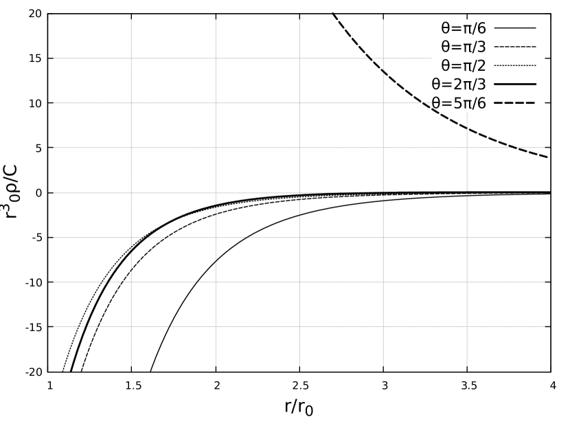
Figure 24: Normalized charge density in equation 137, as a function of $r/r_{0}$ for different $\theta$. Here, $g=1$ was used and $C^{2}=2.33$.

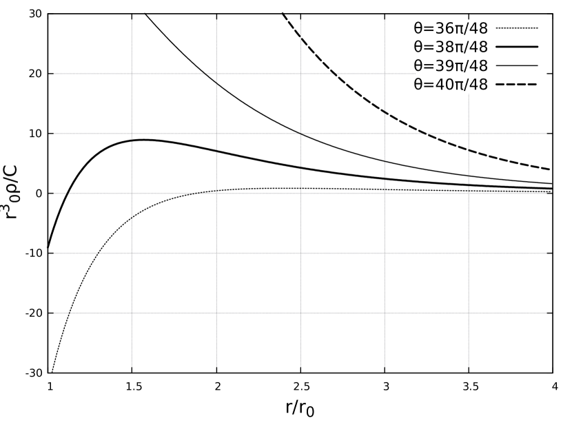
Figure 25: Normalized charge density in equation 137, as a function of $r/r_{0}$ for different $\theta$. Here, $g=1$ was used and $C^{2}=2.33$.

8 Constant scalar potential in a dipole-like spatial distribution

Let us consider a finite region of 3-dimensional space in which the classical scalar potential is constant, i.e.

$$\varphi=V=const.$$ (143)

Equation (20) for the vector potential, a sort of non-Abelian generalization of the Ampère’s Law in the Coulomb Gauge 23, is reduced to the Helmholtz equation, [45]. By neglecting the solutions that diverge in the origin we have the following solution:

$$\vec{A}(\vec{r})= \sum_{l=0}^{\infty}\sum_{m=-l}^{l}j_{l}(gVr)Y^{m}_{l}(\theta,\phi)\left(\hat{r}\left(a_{l}^{m}\sin(\theta)\cos(\phi)+b^{l}_{m}\sin(\theta)\sin(\phi)+c^{l}_{m}\cos(\theta)\right)\right.$$

$$+\left.\hat{\theta}\left(a^{l}_{m}\cos(\theta)\cos(\phi)+b^{l}_{m}\cos(\theta)\sin(\phi)-c^{l}_{m}\sin(\theta)\right)+\hat{\phi}\left(-a^{l}_{m}\sin(\phi)+b^{l}_{m}\cos(\phi)\right)\right),$$ (144)

where $a^{l}_{m},b^{l}_{m}$ and $c^{l}_{m}$ are the integration constants, $j_{l}(x)$ are the spherical Bessel functions and $Y^{m}_{l}(\theta,\phi)$ are the spherical harmonics. Eq. (19), in this case, reduces to:

$$\vec{A}^{2}(\vec{r})\equiv A^{2}(\vec{r})=\frac{\rho(\vec{r})}{2g^{2}V}.$$ (145)

Therefore the constant scalar potential solution is possible provided the color charge density has a very particular shape.

As we can see, since $A^{2}$ is positive, if $V<0$ ($V>0$), then $\rho<0$ ($\rho>0$). With that in mind, we choose to use this solution to a model for a color-anticolor dipole configuration restricted to two semi-spheres with color charges with opposite sign of radius $R_{0}$, by means of the following prescription:

$$\varphi(\vec{r})=V\left(H(-r+R_{0},\theta+\frac{\pi}{2})-H(-r+R_{0},\theta-\frac{\pi}{2})\right),\;\;V>0,$$ (146)

where $H(x)$ is a two dimensional Heaviside function for the coordinates $r$ and $\theta$. Note that, according to 28, this is a model for two pairs of dipoles, i.e. four color charges that create a color-neutral system. This discontinuity may be thought by considering a very tiny region without color charge that separates the two different regions, for $\varphi=+V$ and $\varphi=-V$. Eventual chromo-electromagnetic fluxes in this tiny transition region will be neglected. This sort of configuration would be possible in electromagnetic system for two conducting semi-spheres with superficial charge distribution, being this picture however not suitable for the present Yang Mills system because of strong non-Abelian effects: in spite of being equipotential volumes the chromo-electric fields are not zero. From eq. (145) it corresponds to a dipolar configuration being that in both regions the vector potential $A^{2}(\vec{r})$ is the same. It’s important to notice that $\vec{A}$ can be non-zero only in the region where $\varphi\neq 0$. We can achieve this continuously by imposing that for $r=R_{0}$ one has $\vec{A}=0$. By picking up a single component $l$, this implies:

$$gVR_{0}=Z^{l}_{n},$$ (147)

where $Z^{l}_{n}$ is the $n-$th zero of the spherical Bessel function of order $l$. Some of these zeros are given in table 3.

$l$	$Z^{l}_{1}$	$Z^{l}_{2}$	$Z^{l}_{3}$
1	4.493	7.725	10.904
2	5.764	9.095	12.323
3	6.988	10.417	13.698

Table 3: Zeros for spherical Bessel function, of different lowest orders of $l$.

As an example, consider the lowest solution in $l$ ($l=1$) that is given by:

$$\vec{A}(\vec{r}) = \left(\frac{\sin(gVr)}{(gVr)^{2}}-\frac{\cos(gVr)}{gVr}\right)\cos(\theta)\left(\hat{r}\left(a^{1}\sin(\theta)\cos(\phi)+b^{1}\sin(\theta)\sin(\phi)+c^{1}\cos(\theta)\right)\right.$$ (148)

$$+ \left.\hat{\theta}\left(a^{1}\cos(\theta)\cos(\phi)+b^{1}\cos(\theta)\sin(\phi)-c^{1}\sin(\theta)\right)+\hat{\phi}\left(-a^{1}\sin(\phi)+b^{1}\cos(\phi)\right)\right),\;\;\;\;r\leq R_{0}.$$

By redefining the integration constant:

$$\sqrt{(a^{1})^{2}+(b^{1})^{2}+(c^{1})^{2}}=\frac{1}{r_{0}},$$ (149)

the resulting charge density, c-electric and c-magnetic fields - in the region $r<R_{0}$ - are given by:

$$\rho(\vec{r}) =I_{\rho}\left(\frac{2\;g^{2}V}{r_{0}^{2}}\right)\frac{1+((gVr)^{2}-1)\cos^{2}(gVr)-2gVr\sin(gVr)\cos(gVr)}{(gVr)^{4}}\cos^{2}(\theta),$$ (150)

$$\vec{E}_{a}(\vec{r}) =\frac{gV}{r_{0}}\left(\frac{\sin(gVr)}{(gVr)^{2}}-\frac{\cos(gVr)}{gVr}\right)\cos(\theta)\hat{k}(\delta_{ac}-\delta_{ad}),$$ (151)

$$\vec{B}_{a}(\vec{r}) =\frac{gV}{r_{0}}\cos(\theta)\sin(\theta)\left(\frac{\sin(gVr)(3-(gVr)^{2})-3gVr\cos(gVr)}{(gVr)^{3}}\right)\hat{\phi}(\delta_{ac}+\delta_{ad}),$$ (152)

where the effect of the discontinuity in $\varphi(\vec{r})$, that yields a Dirac-delta function, was omitted. In the above equation for the color-charge density equation it was used:

$$I_{\rho}=\begin{cases}1,\mbox{ for }\theta<\pi/2,\\ -1,\mbox{ for }\theta>\pi/2.\end{cases}$$ (153)

Note that all the cases I,V,U-spin have the same result.

In Figs. (27) and (27) the normalized/dimensionless c-electric field, Eq. (151), and c-magnetic field, Eq. (152) for the lowest $l=1$, are exhibited as a function of the dimensionless variable $gVr$ for different angles $\theta$. The oscillatory behavior must be an indication of the sharp transition between the inner and outer parts of the sphere defined by Eq. (146) that define the dipole-like configuration. The radius of the sphere may be identified with the zero of the color-charge density that is the same as the first zero of the c-electric field. It can be identified with the lowest zero of the Bessel function:

$$R_{0}\simeq\frac{4.493}{gV}.$$ (154)

The c-magnetic field, however, has a finite value at $r=R_{0}$.

In Fig. (28) the corresponding normalized and dimensionless color-charge density is shown as a function of the variable $gVr$. The zero is, of course, at the same point as the first zero of the c-electric field defined above.

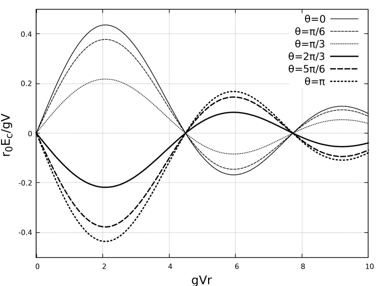
Figure 26: $|\vec{E}_{c}|=E_{c}$ field, Eq. (151), as a function of $gVr$ for different angles $\theta$.

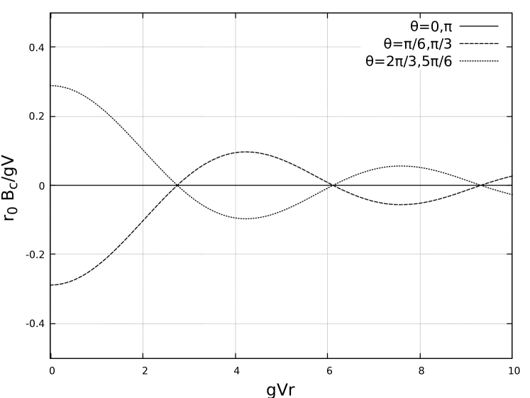
Figure 27: $|\vec{B}_{c}|=B_{c}$ field, eq. (152), as a function of $gVr$ for different angles $\theta$ .

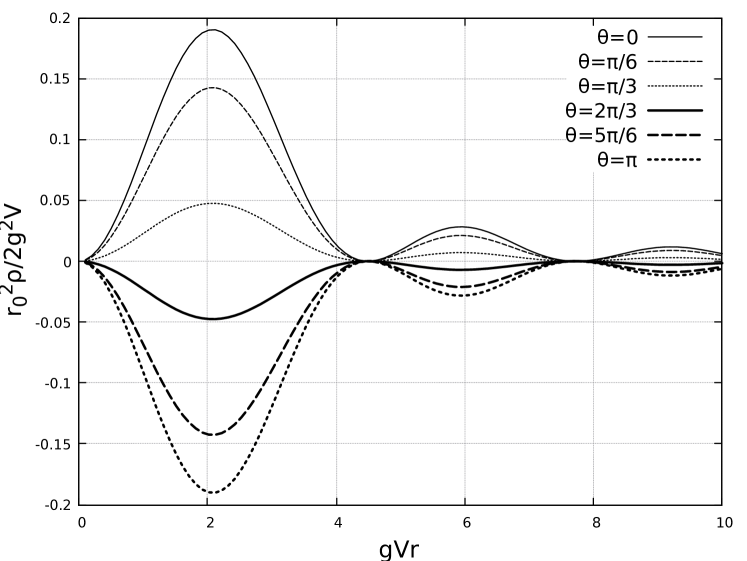
Figure 28: Charge density, eq. (150), as a function of $gVr$ for different angles $\theta$.

8.1 Classical model for a meson

Consider this dipole-type configuration may be associated to a classical model for a meson configuration of radius $R_{0}$ to some extent inspired in the MIT bag model [49]. Eq. (154) suggests that, for $R_{0}\simeq 0.9$ fm and $g=1$, one might have $V\sim 1$ GeV that is approximately a typical energy scale of hadron physics.

The corresponding total energy inside the sphere of radius $R_{0}$ for $l=1$ is obtained by integrating eq. (B.11). It yields the following:

$$U(l=1)=\frac{\pi}{gVr_{0}^{2}}\left(\frac{gVR_{0}}{3}+\frac{\sin(2gVR_{0})}{6}-2\frac{\sin^{2}(gVR_{0})}{3gVR_{0}}+\frac{4}{15}I(gVR_{0})\right),$$ (155)

where:

$$I_{1}(gVR_{0}) =\int_{0}^{gVR_{0}}\frac{\left((3-x^{2})\sin(x)-3x\cos(x)\right)^{2}}{x^{4}}dx.$$ (156)

The total charge contained on the top hemisphere is given by:

$$Q=2\pi\int_{0}^{\pi/2}\int_{0}^{R_{0}}\rho r^{2}\sin(\theta)drd\theta=\frac{\pi}{3g(r_{0}V)^{2}}I_{2}(gVR_{0}),$$ (157)

where:

$$I_{2}(gVR_{0})=\int_{0}^{gVR_{0}}\frac{1+(x^{2}-1)\cos^{2}(x)-2x\sin(x)\cos(x)}{x^{2}}dx.$$ (158)

And it’s clear that for the bottom hemisphere the total charge is given by the same values, times $-1$.

For the values in table (3), the resulting lowest energies and charges are exhibited in Table (4).

	$Z^{1}_{1}$	$Z^{1}_{2}$	$Z^{1}_{3}$
$\frac{gVr_{0}^{2}U({l=1})}{\pi}$	1.998	3.546	5.046
$\frac{3g(r_{0}V)^{2}Q}{\pi}$	2.141	3.7989	5.407

Table 4: Values of the (normalized) energy and charge (top hemisphere) for different zeros of the spherical Bessel function.

Note that the constant of integration is to be associated with a normalization for the vector potential - in Eq. (149), while the normalization for the scalar is given by the constant $V$. So, rewriting $r_{0}$ in therms of $V$, Eq. (154) as:

$$r_{0}V=\epsilon,$$ (159)

where the new constant $\epsilon$ represents an eventual deviation of the vector potential normalization from the scalar one. The following three relations arise:

$$R_{0} =\frac{Z^{l}}{gV};$$ (160)

$$U =\frac{V\pi}{g\epsilon^{2}}F(Z^{l});$$ (161)

$$Q =\frac{\pi}{3g\epsilon^{2}}G(Z^{l}),$$ (162)

where the parameters $F$ and $G$ are the ones in table 4 for a particular zero of the Bessel function $Z^{l}$. The total energy of the configuration may be written as:

$$U=3QV\frac{F(Z^{l})}{G(Z^{l})}=\frac{3Q}{gR_{0}}\frac{Z^{l}F(Z^{l})}{G(Z^{l})}.$$ (163)

The value of the charge $Q$ is associated with the combinations in 28, which are normalized. Then, we may have $Q=1$. The total energy of the classical dipole-configuration, Eq. 163, may be associated to a classical model for tetraquark’s states, two color and two anti-color with total color charge zero. The corresponding energies $U$ for particular $l=1,2,3$ as functions of the radius $R_{0}$ are shown in Fig. (29).

The relation of radius and total energy exhibit values somewhat similar to the ones found the phenomenology of heavy tetraquarks as discussed in Ref [50] and references quoted therein. Masses of mesons candidates to be heavy tetraquarks with at least two charm/anti-charm quarks, $c$ or $\bar{c}$, were measured to be at least 3900 MeV and masses of candidates to heavy tetraquarks, with at least one bottom or anti-bottom quark $b$ or $\bar{b}$, have been found to be larger than at least 10 GeV. Tetraquarks with two quarks $b$, $\bar{b}$ or $\bar{b}b$ to be larger than 11 GeV or with three quarks $b$ of the order of 14- 15 GeV. For charmed meson with three $c$-quarks the typical size of a compact tetraquark is $0.1$ fm whereas a molecule (mesons bound state) has a typical scale of the order of 1 fm.

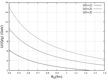
Figure 29: Values of the energy $U/(Q/g)$, equation 163 as a function of $R_{0}$.

9 Summary and conclusions

In this work, some aspects of the $N_{c}=3$ classical Yang-Mills equations, in the Coulomb gauge, were discussed in the presence of color sources in the spherical coordinate system by means of the equations of the $SU(2)$ sub-groups. Although the equations are non-Abelian they contain different limits in which they behave effectively as if they were Abelian, independently of the value of the coupling constant. By assuming the vector and scalar potentials to be fully spherically symmetric, i.e. dependent only on the radial coordinate, the only possible non-trivial solution was found to be given by the Abelian limit. Conversely, by imposing the scalar potential to be spherically symmetric the vector potentials were found to develop strong anisotropies.

Different specific solutions for the scalar potential were considered separately and the consequences were investigated. The charge distributions were left, to some extent, free such that these scalar gauge potential solutions remain valid. The following scalar potentials were considered: the Coulomb potential and an anisotropic extension, a linear potential and a Yukawa potential. Also a sort of dipole-type configuration of constant scalar potential inside a sphere of radius R, being a semi-sphere of positive constant scalar potential $V$ and a semi-sphere of negative $V$. In some situations, the existence of a color charge distribution was associated to a non zero vector potential such as in the case of the Yukawa potential, being that the range of the potential is associated to the typical range of the color-charge distribution. For these cases, outside the region in which color-charge distribution is displaced there are no non-Abelian effects. In some cases therefore, there is a need to impose a maximum radius R where the color-charge distribution remains and for that, a model have been adopted to give further meaning for the resulting configuration. For that, the reasoning of the MIT bag model was considered and it turns out that results might contribute for the dynamical emergence of a bag size. Furthermore, most of the configurations analyzed might contribute to the formation of a classical picture of a constituent quark in the sense of a quark that is dressed by non-Abelian effects being highly anisotropic.

By enforcing the scalar potential to be a Coulomb-potential in the presence of a punctual color-charge and an ad hoc three-dimensional color-charge distribution, and by enforcing the c-electric field Gauss Law to be satisfied, it generates a constraint between the color-charge distribution and the components of the vector potential. Solutions for $\vec{A}(\vec{r})$ were found analytically. A condition for the coupling constant and color-charge normalization was found to be: $0\leq\frac{qg}{4\pi}=\sqrt{l(l+1)-\beta}\leq\frac{1}{2}$ where $l$ is the angular momentum and $\beta$ is a constant of integration. The resulting charge distribution and c-electric and c-magnetic fields contain singularities in the origin being strongly anisotropic. For $\theta=\pi/2$ they reduce to the usual punctual charge and Coulomb potential, being that the magnetic field has a behavior like $1/r^{3}$ in the direction $\hat{\theta}$ - as a purely non-Abelian effect. The c-magnetic field in general, however, presents analytical cuts for $\theta=0,\pi$, besides the singular behavior at $r=0$. The chromo-electric and chromo-magnetic fluxes, and the energy density, are therefore strongly anisotropic. The total charge $Q$ contained inside a sphere of radius $R$ is given by:

$$Q=q\left(1+\frac{g^{2}}{T-1}\left(\frac{r_{0}}{R}\right)^{2(T-1)}\right).$$ (164)

Since $T>1$, for a fixed $R$ the quark color-charge is increased due to the gauge potentials.

A classes of anisotropic extensions of the Coulomb potential were searched to be of the form: $\varphi(r,\theta)=f(\theta)/r$, where $f(\theta)$ was envisaged to have specific shapes. Solutions with $f(\theta)=\frac{\lambda\cos^{n}(\theta)}{\sin(\theta)}$ were found for $n=0$. In this case, analytical solutions were found for the vector potential in the $\hat{\phi}$ direction for the lower angular momenta $l=0,1$ with usual singularity in the origin. However, similarly to the strict Coulomb potential, there appears non-analytical behavior for $\theta=0,\pi$. The corresponding color-charge density presents singularities both at the origin, for $1/r^{n}$ (n=3,4), and cuts in the directions $\theta=0,\pi$. Components of c-electric and c-magnetic fields may change sign at different angles, depending on the angular momenta $l=0,1$ for example for $\theta=\pi/2$ or $\theta=\pi$, and this suggests a (non trivial or asymmetric) dipole-like color-charge configuration that can be naturally associated to the anisotropic Coulomb potential shape. The analytical cuts happen as if a current were passing along these directions $\theta=0,\pi$, but it is rather a static non-spherical non-Abelian effect that may mimic the effect of a color-electric current in terms of the set of Abelian equations of motion. This can also be understood for the other anisotropic solutions with analytical cuts,

By enforcing the gauge scalar potential to have a linearly increasing solution, $\varphi=\kappa r$, by adopting a similar procedure to the one for the Coulomb potential, without the punctual charge, analytical solutions for the vector potential were also found with the corresponding c-electric and c-magnetic fields. They are given by Bessel functions and are strongly oscillatory with the anisotropic behavior. The oscillatory behavior suggests the need of limiting the solution to be valid inside a finite region at the example of bag-like models. The vector potential, c-electric field, and the components of the c-magnetic field disappear not necessarily in the same radial coordinate and the color charge distribution may have zero’s in particular directions, but not all of them, for particular values of the parameters such as $\kappa$ and the field normalization. There are directions in which the color-charge distribution does not go to zero, except in infinite. A precarious dynamical way to define $\kappa$ was proposed by imposing the solution to be valid inside a finite spatial region. By considering a typical distance for which color-charge distribution go to zero for $\gamma\sim 0.1$ it yields $\kappa\sim 0.03$ GeV² that is smaller than lattice results $\sigma_{latt}\sim 0.19$ GeV² [2, 10]. The resulting configuration is therefore strongly anisotropic and the c-electric and c-magnetic fluxes are also strongly anisotropic.

The case of a Yukawa potential for the scalar potential, $\varphi=-\frac{C}{r}e^{r/r_{0}}$, was also addressed being that the length scale $r_{0}$ was dynamically associated to the color-charge distribution. By considering separation of variables for the vector potential, analytical cuts were found in the $\theta-$dependence for angles $\theta=0,\pi$. Only numerical solutions for the radial dependence of the vector potential could be found in this case. For that, singular boundary conditions in the origin were considered and solutions were found as functions of $r/r_{0}$. A determination of $r_{0}$, the range of the Yukawa potential, was not possible although it is traced back to the color-charge distribution. The color-charge distribution is highly anisotropic being that a more drastic behavior happens around the analytical cut at $\theta=\pi$.

Finally, one configuration of positive and negative constant scalar potential, inside two semi-spheres, were defined leading to a sort of dipole type configuration. The oscillatory vector potential presents zeros, from the spherical Bessel function of order l, being that the resulting c-electric and c-magnetic fields fluxes are strongly anisotropic. Whereas the c-electric field has the same zeros of the color-charge distribution the c-magnetic field has its zero at a smaller radial coordinate. By imposing continuity of the solutions, some boundary conditions were chosen. This dipole type configuration inspired a sort of classical bag-model for (heavy) tetraquarks since the dipole configuration for $\varphi$ is directly defined for a combination of two color charges according to the choices in Table (1) for V-spin and U-spin. The masses of the configuration, defined as the total energy of the c-electric and c-magnetic fields, can present the order of magnitude of those measured or predicted for heavy tetraquarks.

Several of the solutions found above for the vector potentials and color-charge distributions were found to be strongly anisotropic with analytical cuts. The chromo-electric and magnetic fluxes in hadrons, mesons and baryons, are necessarily anisotropic and this comparison might suggest that emergence of these anisotropic fluxes of c-electric and c-magnetic lines may be part of the confinement mechanism. As an outcome of this work, it can be stated that, at the classical Yang-Mills level, the gauge scalar potentials that were considered would be more suitably used as long as some further corresponding anisotropic vector potentials and color-charge distributions, are considered. These issues might have relevant effects in the hadron spectroscopy when calculated with Schrodinger or Dirac equation type or Bethe-Salpeter equations modeled with gauge potentials. There are available estimations of the anisotropy’s effects on the gluon propagator [54] however the eventual role of these classical solutions for the full quantum problem is to be understood in the future. Further consequences of the breaking of rotational invariance were not investigated in this work.

Appendix A Appendix A: The equations for $SU(2)$

As pointed out in the previous section, we may reduce the problem from $SU(3)_{c}$ color group to a subgroup sector, given by an $SU(2)_{I,V,U}$. The prescriptions 16 and 17 are now generalized for containing all potentials for the $SU(2)$ case, which is given by the set of equations (for equivalent non-abelian directions, with arguments similar to past section):

$$\nabla^{2}\sigma =-j_{\sigma}$$ (A.1)

$$\nabla^{2}\vec{\sigma} =0;$$ (A.2)

$$\nabla^{2}\varphi-2g^{2}\left(A^{2}\varphi-A^{0}\vec{A}\cdot\vec{\varphi}\right) =-\rho;$$ (A.3)

$$\nabla^{2}\vec{\varphi}+2g^{2}\left(A^{0}\varphi\vec{A}-(A^{0})^{2}\vec{\varphi}+\vec{A}\times\left(\vec{A}\times\vec{\varphi}\right)\right) =0;$$ (A.4)

$$\nabla^{2}A^{0}-g^{2}\left(\vec{\varphi}\cdot\left(\vec{A}\varphi-A^{0}\vec{\varphi}\right)\right) =0;$$ (A.5)

$$\nabla^{2}\vec{A}-g\left(\frac{1}{2}\vec{\nabla}\times\left(\vec{\varphi}\times\vec{A}\right)-\vec{\varphi}\times\vec{\nabla}\times\vec{A}+\varphi\vec{\nabla}A^{0}\right.$$

$$\left.-A^{0}\vec{\nabla}\varphi\right)-g^{2}\left(\frac{1}{2}\vec{\varphi}\times\left(\vec{\varphi}\times\vec{A}\right)+\varphi\left(A^{0}\vec{\varphi}-\vec{A}\varphi\right)\right) =0,$$ (A.6)

where $A^{0}$ stands for the scalar potentials in the non-abelian directions, $\vec{A}$ the non-abelian vector potentials and $\vec{\varphi},\vec{\sigma}$ are the vector correspondents of the scalars found in table 1.

The version of Eqs. (9,10), with time dependence and in Lorentz gauge, is (for U-spin, since the others are completely equivalent):

$$\nabla^{2}\xi =-\sigma;$$ (A.7)

$$\frac{\partial}{\partial t}\vec{\nabla}\xi =\vec{\sigma};$$ (A.8)

$$\nabla^{2}\varphi+4g(\vec{A}_{6}\cdot\frac{\partial}{\partial t}\vec{A}_{7}-\vec{A}_{7}\cdot\frac{\partial}{\partial t}\vec{A}_{6})-4g^{2}(A_{6}^{2}+A_{7}^{2})\varphi =-\rho;$$ (A.9)

$$\frac{\partial}{\partial t}\vec{\nabla}\varphi+4g\left(\vec{\nabla}\times\vec{A}_{6}\times\vec{A}_{7}+\vec{A}_{6}\times\vec{\nabla}\times\vec{A}_{7}\right) =\vec{\rho};$$ (A.10)

$$\frac{\partial}{\partial t}\vec{\nabla}\cdot\vec{A}_{6}+2g\vec{\nabla}\varphi\cdot\vec{A}_{7}+g\varphi\vec{\nabla}\cdot\vec{A}_{7} =j^{0}_{6};$$ (A.11)

$$\frac{\partial}{\partial t}\vec{\nabla}\cdot\vec{A}_{7}-2g\vec{\nabla}\varphi\cdot\vec{A}_{6}-g\varphi\vec{\nabla}\cdot\vec{A}_{6} =j^{0}_{7};$$ (A.12)

$$\vec{\nabla}(\vec{\nabla}\cdot\vec{A}_{6})-\vec{\nabla}^{2}\vec{A}_{6}+\frac{\partial^{2}}{\partial t^{2}}\vec{A}_{6}+g\left(2\varphi\frac{\partial\vec{A}_{7}}{\partial t}+\frac{\partial\varphi}{\partial t}\vec{A}_{7}\right)-g^{2}\varphi^{2}\vec{A}_{6}+4g^{2}\vec{A}_{7}\times\left(\vec{A}_{6}\times\vec{A}_{7}\right) =\vec{j}_{6};$$ (A.13)

$$\vec{\nabla}(\vec{\nabla}\cdot\vec{A}_{7})-\vec{\nabla}^{2}\vec{A}_{7}+\frac{\partial^{2}}{\partial t^{2}}\vec{A}_{7}+g\left(2\varphi\frac{\partial\vec{A}_{6}}{\partial t}+\frac{\partial\varphi}{\partial t}\vec{A}_{6}\right)-g^{2}\phi^{2}\vec{A}_{7}-4g^{2}\vec{A}_{6}\times\left(\vec{A}_{6}\times\vec{A}_{7}\right) =\vec{j}_{7}.$$ (A.14)

Appendix B: Chromo-electric and chromo-magnetic fields

Analogous to the electromagnetic fields, one can define:

$$F_{i0}=E_{i} \rightarrow \vec{E}_{a}=-\frac{\partial\vec{A}_{a}}{\partial t}-\nabla A^{0}_{a}+gf_{a}^{bc}A_{b}^{0}\vec{A}_{c},;$$ (B.1)

$$F_{ij}=\epsilon_{ijk}B_{k} \rightarrow \vec{B}_{a}=\nabla\times\vec{A}_{a}+gf_{a}^{bc}(\vec{A}_{b}\times\vec{A}_{c}),$$ (B.2)

Besides the Euler-Lagrange equations given in the text, a non-Abelian generalization of the Faraday’s law, by choosing $\mu=t,\nu=i,\lambda=j$ in Eq. (10), is obtained from the topological constraint of the SU(3) Lie algebra. It yields: by multiplying by $\epsilon_{ijk}$ and by using $\epsilon_{ijk}\epsilon_{ijl}=2\delta_{kl}$

$$2\partial_{t}B_{k}+2(\nabla\times E)_{k}-ig\left(2[A_{0},B_{k}]+2(A_{j}\times E_{i})_{k}-2(E_{j}\times A_{i})_{k}\right).$$ (B.3)

The set of four equations can be written as:

$$\nabla\cdot\vec{E}_{a}+f_{abc}\vec{E}_{b}\cdot\vec{A}_{c} = g\bar{\psi}\lambda_{a}\gamma^{0}\psi,$$ (B.4)

$$\nabla\times\vec{E}_{a}+f_{abc}(A_{0b}\vec{B}_{b}-\vec{A}_{c}\times\vec{E}_{b}) = -\frac{\partial\vec{B}_{a}}{\partial t}-gf_{abc}A_{b}^{0}\vec{B}_{c},$$ (B.5)

$$\nabla\cdot\vec{B}_{a}+f_{abc}\vec{A}_{c}\cdot\vec{B}_{b}=0,$$ (B.6)

$$\nabla\times\vec{B}_{a}+f_{abc}(\vec{A}_{c}\times\vec{B}_{b}-A_{0c}\vec{E}_{b}) = \frac{\partial\vec{E}_{a}}{\partial t}+g\bar{\psi}\lambda_{a}\vec{\gamma}\psi+gf_{abc}A_{b}^{0}\vec{E}_{c},$$ (B.7)

It is not possible, however, to write these equations solely in terms of $E_{c}$ and $B_{c}$, as it is well known, being needed to account for scalar and vector potentials as well, except in very particular cases.

For the prescriptions adopted in the work for the different components of the gauge scalar and vector potentials, Eq. (16,17), C-Electric and C-Magnetic fields can be written as:

$$\vec{E}_{a}= \left(-\vec{\nabla}A^{0}_{3}\right)\delta_{a3}+\left(-\vec{\nabla}A^{0}_{8}\right)\delta_{a8}+\left(-\vec{\nabla}A^{0}-g\left(\vec{\varphi}A^{0}-\varphi\vec{A}\right)\right)\delta_{ac}+\left(-\vec{\nabla}A^{0}+g\left(\vec{\varphi}A^{0}-\varphi\vec{A}\right)\right)\delta_{ad},$$ (B.8)

$$\vec{B}_{a}= \left(\vec{\nabla}\times\vec{A}_{3}\right)\delta_{a3}+\left(\vec{\nabla}\times\vec{A}_{8}\right)\delta_{a8}+\left(\vec{\nabla}\times\vec{A}+g\vec{\varphi}\times\vec{A}\right)\delta_{ac}+\left(\vec{\nabla}\times\vec{A}-g\vec{\varphi}\times\vec{A}\right)\delta_{ad}.$$ (B.9)

Energy-momentum tensor and Continuity equations

The gauge-invariant traceless energy-momentum tensor by omitting quarks contributions to avoid the problem of the energy of a single quark-source, or its size, can be written as:

$$\theta^{\mu\nu}=\frac{1}{2}\mbox{Tr}(-F^{\mu\rho}F_{\rho}^{\nu}+\frac{1}{4}g^{\mu\nu}F^{\rho\sigma}F_{\rho\sigma}).$$ (B.10)

The most relevant two components are the energy density and pressure that can be written in general in terms of the chromo-electric and chromo-magnetic fields, $\vec{E}_{c}$ and $\vec{B}_{c}$, defined as usual in the Appendix (Appendix B: Chromo-electric and chromo-magnetic fields). By adding the quark current it can be written that:

$$\theta^{00} = \frac{1}{2}(\vec{E}_{a}\cdot\vec{E}_{a}+\vec{B}_{a}\cdot\vec{B}_{a})+j^{i}_{a}A^{a}_{i}$$ (B.11)

$$\theta^{0i} = (\vec{E}_{a}\times\vec{B}_{a})_{i},$$ (B.12)

$$\theta_{ij} = -E_{i}^{a}E_{j}^{a}-B_{i}^{a}B_{j}^{a}+\frac{\delta_{ij}}{2}(\vec{E}_{a}\cdot\vec{E}_{a}+\vec{B}_{a}\cdot\vec{B}_{a}).$$ (B.13)

From the Noether Current defined in 6, we may write the continuity equations as:

$$\frac{\partial j^{0}_{a}}{\partial t}+\vec{\nabla}\cdot\vec{j}_{a}+gf_{abc}\left(A^{0}_{b}j^{0}_{c}-\vec{A}_{b}\cdot\vec{j}_{c}\right)=0.$$ (B.14)

References

- [1] C.N. Yang, R.L. Mills, Conservation of Isotopic Spin and Isotopic Gauge Invariance, Phys. Rev. 96, 191 (1954).
- [2] W.N. Cottingham, D.A. Greenwood, An Introduction to the Standard Model of Particles, 2nd Ed. Cambridge (2007).
- [3] T.P. Cheng, L.F. Li, Gauge Theory of Elementary Particles, Oxford (1984).
- [4] L. O’Raifeartaigh, N. Straumann, Gauge theory: Historical origins and some modern developments, Rev. of Mod. Phys. 72, 1 (2000).
- [5] P. Rossi, Exact Results in the Theory of non-Abelian magnetic monopoles, Phys. Rept. 86, 317 (1982).
- [6] A. Actor, Classical solutions of SU(2) Yang-Mills theories, Rev. of Mod. Phys. 51, 461 (1979).
- [7] T.T. Wu, and C. N. Yang, 1968, in Properties of Matter Under Unusual Conditions, edited by H. Mark and S. Fernbach (Interscience, New York). Rosen, G., 1972, J. Math. Phys. 13, 595.
- [8] G. ’t Hooft, Magnetic monopoles in unified gauge theories. Nuclear Physics B 79, 276 (1974). A. M. Polyakov, Particle spectrum in the quantum field theory. JETP Letters 20, 194 (1974). G. ’t Hooft, F. Bruckmann, Monopoles, Instantons and Confinement, arXiv:hep-th/0010225.
- [9] E. Elizalde, Phys. Lett. B77, 73 (1978).
- [10] G. Bali, QCD forces and heavy quark bound states, Phys.Rept.343, 1 (2001).
- [11] N. Brambilla, et al, QCD and strongly coupled gauge theories: challenges and perspectives, Eur. Phys. J. C 74, 2981 (2014).
- [12] D. Griffiths, Introduction to Elementary Particles, Wiley, (1987).
- [13] P. Sikivie, N. Weiss, Classical Yang-Mills theory in the presence of external sources Phys. Rev. D 18, 3809 (1978).
- [14] P. Sikivie, N. Weiss, Screening Solutions to Classical Yang-Mills Theory, Phys. Rev. Lett. 40, 1411 (1978).
- [15] J.E. Mandula, Classical Yang-Mills potentials, Phys. Rev. D14, 3497 (1976)
- [16] R. Jackiw, L. Jacobs, C. Rebbi, Static Yang-Mills fields with sources, Phys. Rev. D20, 474 (1979).
- [17] S. M. Mahajan, P.M. Valanju, Finite-energy classical solutions to Yang-Mills theories, Phys. Rev. D35, 2543 (1987)
- [18] R. E. Crandall, D. J. Griffiths, N. A. Wheeler, R. A. Mayer Fields of an infinite plane of color, Phys. Rev. D25, 1143 (1982)
- [19] L. Mathelitsch, H. Mitter, F. Widder, Stationary Yang-Mills fields with current sources, Phys. Rev. D 25, 1123 (1982)
- [20] G. Passarino, Yang-Mills theories in the presence of classical plane-wave fields: stability properties, Phys. Lett. B 176, 135 (1986)
- [21] A. Tsapalis, E. P. Politis, X. N. Maintas, and F. K. Diakonos, Gauss’ law and nonlinear plane waves for Yang-Mills theory Phys. Rev. D93, 085003 (2016)
- [22] M. Ikeda, Y. Miyachi, On the Static and Spherically Symmetric Solutions of the Yang-Mills Field, Progress of Theoretical Physics 27, 474 (1962).
- [23] T.N. Tudron, Instability of constant Yang-Mills fields generated by constant gauge potentials, Phys. Rev. D22, 2566 (1980)
- [24] S. Huang and A. R. Levi, Phys. Rev. D49, 6849 (1994); A. R. Levi, subtleties and fancies in gauge theory nontrivial vacuum, hep-lat/9409002.
- [25] G.K. Savvidy, Phys. Lett. B71, 133 (1977). S.G. Matinyan and G.K. Savvidy, Nucl. Phys. B134, 539 (1978) N.K. Nielsen and P. Olesen, Nucl. Phys. B144, 376 (1978). J. Ambjorn, N.K. Nielsen and P. Olesen, Nucl. Phys. B152, 75 (1979). J. Ambjorn, P. Olesen, Nucl. Phys. BI70, 60 (1980).
- [26] M. Reuter, C. Wetterich, Search for the QCD ground state, Phys. Lett. B 334, 412 (1994).
- [27] R.A. Coimbra, O. Oliveira, Heavy quarkonia from classical SU(3) Yang Mills configurations, Eur. Phys. J. A 31, 718 (2007)
- [28] A. Kovner, L. McLerran, H. Weigert, Gluon production from non-Abelian Weizsacker-Williams fields in nucleus-nucleus collisions, Phys. Rev. D52, 6231 (1995).
- [29] S. Bazak, S. Mrowczynski, Stability of Classical Chromodynamic Fields, Phys. Rev. D 105, 034023 (2022).
- [30] B. Schenke, S. Schlichting, R. Venugopalan, Azimuthal anisotropies in p+Pb collisions from classical Yang-Mills dynamics, Phys. Lett. B747, 76 (2015).
- [31] O. Philipsen, B. Wagenbach, S. Zafeiropoulos, From the colour glass condensate to filamentation: systematics of classical Yang–Mills theory, Eur. Phys. J. C 79, 286 (2019).
- [32] H. Matsuda, et al, Shear viscosity of a classical Yang-Mills field, Phys. Rev. D102, 114503 (2020).
- [33] M. Frasca, Confinement in a three-dimensional Yang–Mills theory, Eur. Phys. J. C 77:255, (2017)
- [34] J. Greensite, An Introduction to the Confinement Problem, Springer, Lectures notes in Physics 821, (2011).
- [35] J.W. Flower, S.W. Otto, The field distribution in SU(3) lattice gauge theory, Phys. Lett 160B, 128 (1985) R. Sommer, Nucl. Phys. B291 (1986) 673. G. S. Bali, C. Schlichter and K. Schilling, Phys. Rev. D51 (1995) 5165.
- [36] R. W. Haymaker, V. Singh and Y. Peng, Phys. Rev. D53 (1996) 389. M. Luscher, G. Munster, P. Weisz, How thick are chromo-electric flux tubes?, Nucl. Phys. B180, 1 (1981).
- [37] F. Okihary, R. Woloshyn, A study of colour field distributions in the baryon, Nucl. Phys. B 129-130(Proc.Suppl.), 745 (2004). J. Flower, CALT-68-1378 (1986). H. Ichie, V. Bornyakov, T. Streuer and G. Schierholz, Nucl. Phys. B (Proc. Suppl.) 119 (2003) 751, hep-lat/0212036.
- [38] C. Cardona, T. Vachaspati, Instability of a uniform electric field in pure non-Abelian Yang-Mills theory, Phys. Rev. D 104, 045009 (2021).
- [39] P. Sikivie, Instability of Abelian field configurations in Yang-Mills theory, Phys.Rev. D20, 877 (1979).
- [40] S. J. Chang, N. Weiss, Instability of constant Yang-Mills fields Phys. Rev. D 20, 869 (1979).
- [41] O.W. Greenberg, Quarks, Ann. Rev. Nucl. Part. Sci. 28, 327 (1978).
- [42] P. Moon, D.E. Spencer, The meaning of the vector Laplacian, Journal of the Franklin Institute 256, 6 (1953).
- [43] A. Hadicke, H.-J. Pohle, Solutions of the SU(3) gauge field equations with spherical symmetry, Phys. Lett. B137, 193 (1984)
- [44] H.G. Loss, The range of gauge fields, Nucl. Phys. 72, 677 (1965).
- [45] E. Butkov, Mathematical Physics, (1983).
- [46] D. J. Gross and F. Wilczek, Ultraviolet behavior of nonabelian gauge theories, Phys. Rev. Lett. 30, 1343 (1973); H. D. Politzer, Reliable perturbative results for strong interactions?, Phys. Rev. Lett. 30, 1346 (1973).
- [47] A. Deur, S. J. Brodsky, G. F. de Teramond, he QCD Running Coupling, Prog. Part. Nuc. Phys. 90 1 (2016).
- [48] V. Rubakov, Classical Theory of Gauge Fields, translated S.S. Wilson, Princeton (2002).
- [49] A. Chodos, R. L. Jaffe, K. Johnson, C. B. Thorn, V. F. Weisskopf, New extended model of hadrons, Phys. Rev. D 9, 3471 (1974). A. Chodos, R. L. Jaffe, K. Johnson, C. B. Thorn, Baryon structure in the bag theory, Phys. Rev. D 10, 2599 (1974).
- [50] X.-Z. Weng, W.-Z. Deng, S.-L. Zhu, Triply heavy tetraquark states, Phys. Rev. D 105, 034026 (2022).
- [51] R. E. Crandall, D. J. Griffiths, N. A. Wheeler, R. A. Mayer Fields of an infinite plane of color, Phys. Rev. D25, 1143 (1982)
- [52] S. M. Mahajan, P.M. Valanju, Finite-energy classical solutions to Yang-Mills theories, Phys. Rev. D35, 2543 (1987)
- [53] L. Mathelitsch, H. Mitter, F. Widder, Stationary Yang-Mills fields with current sources, Phys. Rev. D 25, 1123 (1982)
- [54] Y. Nakagawa, A. Nakamura, T. Saito, H. Toki, Scaling study of the gluon propagator in Coulomb gauge QCD on isotropic and anisotropic lattices, Phys. Rev. 83, 114503 (2011).