Spin ice in a general applied magnetic field: Kasteleyn transition, magnetic torque and rotational magnetocaloric effect

Abstract

Spin ice is a paradigmatic frustrated system famous for the emergence of magnetic monopoles and a large magnetic entropy at low temperatures. It exhibits unusual behavior in the presence of an external magnetic field as a result of the competition between the spin ice entropy and the Zeeman energy. Studies of this have generally focused on fields applied along high symmetry directions: $[111]$, $[001]$, and $[110]$. Here we consider a model of spin ice with external field in an arbitrary direction. We find that the Kasteleyn transition known for $[001]$ fields, appears also for general field directions and calculate the associated Kasteleyn temperature $T_{K}$ as a function of field direction. $T_{K}$ is found to vanish, with a logarithmic dependence on field angle, approaching certain lines of special field directions. We further investigate the thermodynamic properties of spin ice for $T>T_{K}$, using a Husimi cactus approximation. As the system is cooled towards $T_{K}$ a large magnetic torque appears, tending to align the $[001]$ crystal axis with the external field. The model also exhibits a rotational magnetocaloric effect: significant temperature changes can be obtained by adabiatically rotating the crystal relative to a fixed field.

I Introduction

Spin ice exemplifies much of what is interesting about frustrated systems Harris et al. (1997); Balents (2010); Henley (2010); Castelnovo et al. (2012). The co-existence of a large quasi-degeneracy of ground states Ramirez et al. (1999); Melko and Gingras (2004); Isakov et al. (2005); Giblin et al. (2018) and strong correlations Bramwell et al. (2001); Isakov et al. (2004a); Yavors’kii et al. (2008); Fennell et al. (2009); Kanada et al. (2002) sets the stage for the emergence of exotic excitations: namely, magnetic monopoles Castelnovo et al. (2008); Morris et al. (2009); Jaubert and Holdsworth (2009); Kadowaki et al. (2009); Ryzhkin et al. (2013); Kaiser et al. (2018); Dusad et al. (2019); Samarakoon et al. (2022). The discovery of spin ice also served as an early example of a theme which has grown in importance in the years since: the interplay of frustration and anisotropy Fukazawa et al. (2002).

Magnetic anisotropy is the root of how spin ice can be frustrated, despite dominantly ferromagnetic interactions Bramwell and Harris (1998); Moessner (1998). The importance of anisotropy is also seen through the diverse behaviors induced by applying a magnetic field along different crystal directions. Fields along $\langle 111\rangle$ induce an effectively two-dimensional, disordered, “kagome ice” state Moessner and Sondhi (2003); Hiroi et al. (2003a); Sakakibara et al. (2003); Isakov et al. (2004b); fields along $\langle 110\rangle$ induce a division of the system into effectively one-dimensional chains Hiroi et al. (2003b); Clancy et al. (2009); Guruciaga et al. (2016); Placke et al. (2020); while a field along $\langle 100\rangle$ drives a Kasteleyn transition to an ordered state Powell and Chalker (2008); Jaubert et al. (2008, 2009). Most studies of spin ice in an applied field have focused on fields oriented along Hiroi et al. (2003a); Sakakibara et al. (2003); Isakov et al. (2004b); Hiroi et al. (2003b); Clancy et al. (2009); Guruciaga et al. (2016); Placke et al. (2020); Powell and Chalker (2008); Jaubert et al. (2008, 2009); Harris et al. (1998); Pili et al. ; Baez and Borzi (2016), or close to Moessner and Sondhi (2003); Fennell et al. (2007), those high symmetry directions. Here we give an account of the physics of an idealized spin ice model, with a completely general direction of external field.

We determine the ground state phase diagram as a function of applied field, showing that for non-fine-tuned choices of field direction there is a unique ground state with magnetisation along a $\langle 100\rangle$ axis. At finite temperature, there is a Kasteleyn transition at $T=T_{K}$, separating the field induced order at $T<T_{K}$ from a Coulomb phase at $T>T_{K}$. We determine the dependence of $T_{K}$ on the field direction, showing that it approaches zero in a singular fashion near the boundaries of the ground state phase diagram.

We then go on to study the thermodynamics of the system at $T>T_{K}$ using a Husimi tree approximation. Our account of the thermodynamics is focussed on the effects of applying an external field which is not aligned with a high symmetry direction of the crystal. We find that a large magnetic torque develops as $T_{K}$ is approached from above, as the exchange energy forces the system to align the magnetisation closer to a $\langle 100\rangle$ axis and away from the magnetic field. Relatedly, we find a rotational magnetocaloric effect, in which large changes in temperature can be driven by adiabatic rotation of the crystal relative to the field.

The conventional magnetocaloric effect (MCE) – change in temperature driven by a change in applied field strength – has long been known as a useful probe of frustrated magnetic systems Zhitomirsky (2003); Kohama et al. (2012); Tokiwa et al. (2013); Manni et al. (2014), including spin ice Aoki et al. (2004); Orendáč et al. (2007), and as a potential basis for cleaner refrigeration technology Pecharsky and Gschneidner (1997); Gschneidner and Pecharsky (2008); Balli et al. (2017). By contrast, the rotational magnetocaloric effect (RMCE) has begun to attract significant attention only relatively recently. The RMCE could present certain technological advantages over the conventional MCE Balli et al. (2014, 2017) and recent developments in measurement techniques make it increasingly practical to use RMCE as a probe of novel physics in anisotropic frustrated systems Kittaka et al. (2018, 2021). Here we will show that an idealized model of spin ice predicts an appreciable RMCE, and that interactions enhance the RMCE by an order of magnitude above what would be expected from a simple paramagnet with the same symmetry and single-ion anisotropy.

The Article is organized as follows: in Section II we introduce the model and determine the ground state phase diagram; in Section III we calculate the Kasteleyn temperature. $T_{K}$, as a function of field direction; in Section IV we discuss the thermodynamics at $T>T_{K}$ including the magnetic torque and RMCE; before concluding in Section V.

II Model and Ground states

We consider a nearest-neighbor model for spin ice

$$H=-J\sum_{\left\langle{i,j}\right\rangle}\vec{S}_{i}\cdot\vec{S}_{j}-\vec{h}\cdot\sum_{i}\vec{S}_{i}-D_{\rm SI}\sum_{i}\left(\vec{S_{i}}\cdot\vec{e}_{i}\right)^{2}$$ (1)

where the first term is a ferromagnetic nearest neighbor exchange interaction, the second term is the Zeeman energy and the third term is an easy-axis single-ion anisotropy. Throughout this Article, we take $D_{SI},J>0$ and consider the limit $D_{SI}\gg J\gg h$.

The strong easy-axis anisotropy $D_{SI}\gg J$ aligns the direction of the classical spin $\vec{S}_{i}$ with the line connecting the centers of the two tetrahedra sharing site $i$ [Fig. 1]. The four spins in a unit cell have different easy-axis directions $\vec{e}_{i}$. Numbering the sites in a unit cell from 1 to 4, we choose coordinates where:

$$\vec{e}_{1}=\begin{pmatrix}\frac{1}{\sqrt{3}}\\ \frac{1}{\sqrt{3}}\\ \frac{1}{\sqrt{3}}\\ \end{pmatrix},\ \vec{e}_{2}=\begin{pmatrix}\frac{1}{\sqrt{3}}\\ -\frac{1}{\sqrt{3}}\\ -\frac{1}{\sqrt{3}}\\ \end{pmatrix},\$$

$$\vec{e}_{3}=\begin{pmatrix}-\frac{1}{\sqrt{3}}\\ \frac{1}{\sqrt{3}}\\ -\frac{1}{\sqrt{3}}\\ \end{pmatrix},\ \vec{e}_{4}=\begin{pmatrix}-\frac{1}{\sqrt{3}}\\ -\frac{1}{\sqrt{3}}\\ \frac{1}{\sqrt{3}}\\ \end{pmatrix}$$ (2)

Each spin thus has two orientations, which we can parameterise using an Ising variable $\sigma_{i}$:

$$\vec{S}_{i}=\sigma_{i}\vec{e}_{i}$$ (3)

Using that $\vec{e}_{i}\cdot\vec{e}_{j}=-\frac{1}{3}$ for neighboring sites $i,j$, and dropping an unimportant constant term, the Hamiltonian becomes:

$$H=\frac{J}{6}\sum_{\Delta}\left(\sum_{i\in\Delta}\sigma_{i}\right)^{2}-\sum_{i}\sigma_{i}\left(\vec{h}\cdot\vec{e}_{i}\right)$$ (4)

Here $\Delta$ indexes tetrahedra in the pyrochlore lattice. We see that for $J\gg h$, the ground state must be one in which $\sigma_{i}$ sums to zero on each tetrahedron or, equivalently, where each tetrahedron has two spins pointing in, and two pointing out. This is the “ice rule”, illustrated in Fig. 1. We will work in a limit where $J\rightarrow\infty$, and the ice rule will be absolutely obeyed.

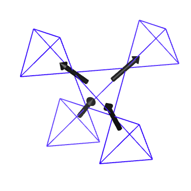
Figure 1: The 2-in-2-out ‘ice-rule’ obeyed by spin-ice on the pyrochlore lattice. All tetrahedra must obey this rule as long as the energy scale associated with the ferromagnetic exchange interaction $J$ is much larger than $T$ and $h$.

The lattice structure in Fig. 1 shows tetrahedra of two orientations. We will refer to these as ‘A’ and ‘B’ tetrahedra. The Zeeman term of the Hamiltonian can be expressed as a sum over ‘A’ tetrahedra:

$$H=\sum_{\Delta\in A}\left[\frac{J}{6}\left(\sum_{i\in\Delta}\sigma_{i}\right)^{2}-\sum_{i\in\Delta}\sigma_{i}\left(\vec{h}\cdot\vec{e}_{i}\right)\right]+$$

$$\qquad\qquad\sum_{\Delta\in B}\frac{J}{6}\left(\sum_{i\in\Delta}\sigma_{i}\right)^{2}$$ (5)

Parametrising the direction of the external field with angles $\theta$ and $\varphi$:

$$\vec{h}=\begin{pmatrix}\cos(\varphi)\sin(\theta)\\ \sin(\varphi)\sin(\theta)\\ \cos(\theta)\end{pmatrix}$$ (6)

and using Eq. (2), we have that for one ‘A’ tetrahedron, the Zeeman energy is:

$$H_{Z}=-\frac{h}{\sqrt{3}}\sigma_{1}\left[\sin(\theta)\cos(\varphi)+\sin(\theta)\sin(\varphi)+\cos(\theta)\right]\\ -\frac{h}{\sqrt{3}}\sigma_{2}\left[\sin(\theta)\cos(\varphi)-\sin(\theta)\sin(\varphi)-\cos(\theta)\right]\\ -\frac{h}{\sqrt{3}}\sigma_{3}\left[-\sin(\theta)\cos(\varphi)+\sin(\theta)\sin(\varphi)-\cos(\theta)\right]\\ -\frac{h}{\sqrt{3}}\sigma_{4}\left[-\sin(\theta)\cos(\varphi)-\sin(\theta)\sin(\varphi)+\cos(\theta)\right]$$ (7)

We can then find the ground state spin configuration as a function of $\theta$ and $\varphi$ for a single $A$ tetrahedron. Where this single tetrahedron ground state is non-degenerate, the ground state of the whole lattice is then found simply by tiling the single tetrahedron ground state over all ‘A’ tetrahedra. One only needs to check that this tiling does not induce a violation of the ice rule on the ‘B’ tetrahedra, but this can readily be verified.

Where the ground state of the ‘A’ tetrahedra is degenerate, there may be many ways to tile the single tetrahedron ground states across the lattice, while maintaining consistency with the ice rule on the ‘B’ tetrahedra.

A phase diagram, mapping out the ground states for general field directions with $h\ll J$ is shown in Fig. 2. There are 6 distinct phases which occupy a finite area of the phase diagram, which are labelled by their magnetisation direction. They correspond to uniform tilings across the lattice of each of the six possible single-tetrahedron ice-rule states.

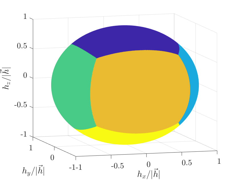
Figure 2: Magnetic ground state phase diagram as a function of external field direction. (a) Phase diagram in the $\theta$-$\varphi$ plane [Eq. (6)]. (b) Phase diagram mapped onto the unit sphere. Each phase is labelled with the direction of the magnetisation in the ground state. The spin configurations in each phase are simply related to one another by rotation of the entire system, and the full physics can be investigated by considering just one of these phases and its boundaries.

The phase diagram contains lines along which two single tetrahedron ground states are degenerate. Along these lines the system splits into two sets of independent 1D chains $\alpha$ and $\beta$. The configuration on the $\alpha$ chains is fixed by the applied field, whereas each $\beta$ chain has an independent two-fold degeneracy. This is well known for the case of a $\langle 110\rangle$ field Hiroi et al. (2003b); Clancy et al. (2009); Guruciaga et al. (2016); Placke et al. (2020). It is interesting to note that the chain degeneracy actually persists along a line of field directions including, but not limited to, the $\langle 110\rangle$ case.

The points on the phase diagram where three single tetrahedron ground states become degenerate correspond to $\langle 111\rangle$ fields, and the well studied case of kagome ice Hiroi et al. (2003a); Udagawa et al. (2002); Moessner and Sondhi (2003). In this case, the system splits into independent kagome planes, and their remains an extensive residual entropy.

For the remainder of this paper we will principally consider the generic case, where the single tetrahedron ground state is non-degenerate, although we will also note the behavior approaching the degenerate limits.

III Kasteleyn Transition Temperature

In this section we consider the finite-temperature phase transition between the field induced ordered phase and the Coulomb phase. This transition is a Kasteleyn transition, and has been studied previously for the case of spin ice in a $\langle 001\rangle$ field Powell and Chalker (2008); Jaubert et al. (2008), and fields close to the $\langle 111\rangle$ direction Moessner and Sondhi (2003). Here we give a generalisation of this to field directions not aligned with a high symmetry direction of the crystal.

We consider field directions such that the largest of the three components of $\vec{h}$ is the $z$-component. In this case, the ground state has magnetisation along the $[001]$ direction [see Fig. 2]. Results for other directions can be obtained straightforwardly by applying cubic rotations to this case.

The ground state is a configuration in which every tetrahedron is in the same 2-in-2-out state with magnetisation along $[001]$. Because we take $J\to\infty$ and do not allow violations of the ice rule, excitations are not single spin flips, but extended strings of flipped spins, spanning the entire system [Fig. 3]. If ice rule violating tetrahedra are allowed, the sharp Kasteleyn transition discussed below becomes a crossover.

The energy cost of a string excitation is proportional to its length, because every flipped spin increases the Zeeman energy. Therefore, at sufficiently low temperature, string excitations are completely suppressed in the thermodynamic limit.

However, the entropy of the string is also proportional to its length, because at every successive layer through the system the string can go one of two ways. The total free energy therefore has competing contributions, and at some finite temperature $T_{K}$, the sign of the free energy per unit length of string changes. For $T>T_{K}$, introducing strings decreases the free energy and strings therefore proliferate, destroying the ordered state. This is the Kasteleyn transition.

For a general magnetic field direction, where the Zeeman energy is not the same for all sites, the energy of the string depends on the path it takes through the system. This is different to the case of the $[001]$ field where all string paths have the same energy per unit length Jaubert et al. (2008); Powell and Chalker (2008). This has to be taken into account when constructing the string free energy.

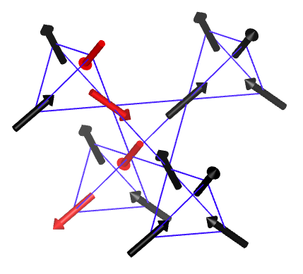
Figure 3: A spin configuration containing a string excitation. The string (highlighted in red) spans the entire system, and costs energy proportional to the linear system size.

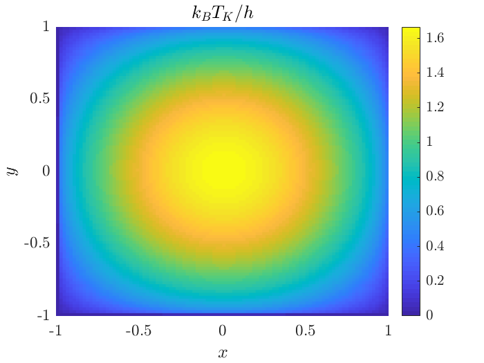
Figure 4: Variation of the Kasteleyn temperature as a function of field direction. The Kasteleyn temperature is given in units of $h/k_{B}$. The centre of the plot corresponds to the [001] field direction, where the result $T_{K}=\frac{2h}{\sqrt{3}\log{2}}$ is reproducedPowell and Chalker (2008). The mapping between the x-y coordinates and $\theta$ and $\varphi$ is given in Eqs. (12)-(15). $T_{K}$ approaches zero at the edge of the plot, which corresponds to the phase boundaries of Fig. 2.

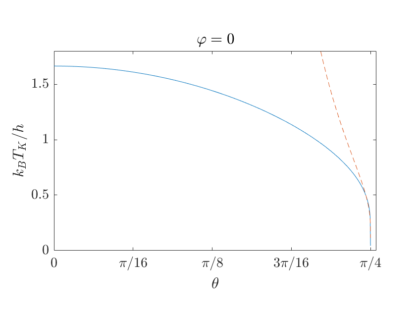
(a)

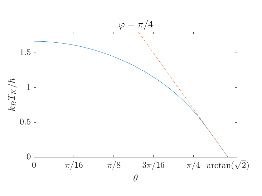
(b)

Figure 5: Variation of the Kasteleyn transition temperature as a function of field angle $\theta$ for $\varphi=0$ [(a)] and $\varphi=\frac{\pi}{4}$ [(b)]. The dashed lines show the asymptotic behavior of $T_{K}$ approaching the magnetic phase boundaries of Fig. 2, as predicted by Eq. (20) for $\varphi=0$ and Eq. (23) for $\varphi=\frac{\pi}{4}$. $T_{K}$ vanishes as $\frac{-1}{\log(\delta)}$ approaching the phase boundaries for generic values of $\varphi$, including $\varphi=0$, where $\delta$ is the distance from the phase boundary. For the special case $\varphi=\frac{\pi}{4}$, $T_{K}$ vanishes linearly towards the kagome ice pointMoessner and Sondhi (2003) at $\theta=\arctan(\sqrt{2})$.

In general, each of the four sites in the pyrochlore unit cell has a different Zeeman energy. Dividing the system into layers normal to the $[001]$ direction, sites with spins in two of these sublattices share one layer, and sites with spins in the remaining two sublattices share the next.

We construct the partition function for a single two layers at a time. Considering all the paths a string could take through two consecutive layers, the two layer partition function is:

$$Z_{2}=2\exp\left(-\frac{-4h\beta}{\sqrt{3}}\cos{\theta}\right)\left\{\cosh\left(\frac{4h\beta}{\sqrt{3}}\sin(\theta)\cos(\varphi)\right)\right.\\ \left.+\cosh\left(\frac{4h\beta}{\sqrt{3}}\sin(\theta)\sin(\varphi)\right)\right\}$$ (8)

From this we can calculate the free energy of a string excitation per two segments:

$$F=\frac{4h}{\sqrt{3}}\cos{\theta}-\frac{1}{\beta}\log(2)\\ -\frac{1}{\beta}\log\left(\cosh\left(\frac{4h\beta}{\sqrt{3}}\sin(\theta)\cos(\varphi)\right)\right.\\ \left.+\cosh\left(\frac{4h\beta}{\sqrt{3}}\sin(\theta)\sin(\varphi)\right)\right)$$ (9)

Setting $F=0$ we find the following expression for $\beta_{K}=\frac{1}{k_{B}T_{K}}$

$$\frac{4h}{\sqrt{3}}\cos{\theta}-\frac{1}{\beta_{K}}\log(2)\\ -\frac{1}{\beta_{K}}\log\left(\cosh\left(\frac{4h\beta_{K}}{\sqrt{3}}\sin(\theta)\cos(\varphi)\right)\right.\\ \left.+\cosh\left(\frac{4h\beta_{K}}{\sqrt{3}}\sin(\theta)\sin(\varphi)\right)\right)=0.$$ (10)

Taking the limit $\theta=0$, Eq. (10) reproduces the known result Powell and Chalker (2008) for the case of $\vec{h}\parallel[0,0,1]$:

$$k_{B}T_{K}(\theta=0)=\frac{2h}{\sqrt{3}\log(2)}.$$ (11)

For more general field directions, Eq. (10) can be solved numerically to obtain the dependence of $T_{K}$ on the applied field direction. This is shown in Figs. 4 and 5. In these figures we make use of the following parameterisation for the angles $\theta$ and $\varphi$, understood as projecting points on the unit sphere onto one face of a unit cube circumscribing it.

$$x= \tan(\theta)\cos(\varphi)$$ (12)

$$y= \tan(\theta)\sin(\varphi)$$ (13)

$$\tan(\varphi)= \frac{y}{x}$$ (14)

$$\cos(\theta)= \frac{1}{\sqrt{x^{2}+y^{2}+1}}$$ (15)

This mapping transforms the magnetic phase boundaries of Fig. 2 onto the edges of the cube.

$T_{K}$ actually vanishes at these phase boundaries. This can be seen by taking the limit $T_{K}\ll h$ in Eq. (10):

$$\frac{4h}{\sqrt{3}}\cos\theta-k_{B}T_{K}\log\bigg{\{}\bigg{[}\exp\bigg{(}\frac{4h}{\sqrt{3}k_{B}T_{K}}\sin(\theta)|\cos(\varphi)|\bigg{)}+$$

$$\exp\bigg{(}\frac{4h}{\sqrt{3}k_{B}T_{K}}\sin(\theta)|\sin(\varphi)|\bigg{)}\bigg{]}\bigg{\}}=0$$ (16)

Considering first the case $|\cos(\varphi)|>|\sin(\varphi)|$, the logarithm can be expanded to obtain for $T_{K}\ll h$ to obtain:

$$\frac{4h}{\sqrt{3}}(\cos\theta-\sin(\theta)|\cos(\varphi)|)$$

$$-k_{B}T_{K}\exp\bigg{(}-\frac{4h}{\sqrt{3}k_{B}T_{K}}\sin(\theta)\big{(}|\cos(\varphi)|-|\sin(\varphi)|\big{)}\bigg{)}$$

$$=0$$ (17)

from which we can see that $T_{K}$ vanishes when

$$\cos(\theta)=\sin(\theta)|\cos(\varphi)|.$$ (18)

Detuning $\theta$ away from this phase boundary gives by an amount $\delta$, gives rise to a logarithmic behavior $T_{K}\sim\frac{1}{\log\left(\frac{1}{\delta}\right)}$. To see this, we define $\theta_{0}(\varphi)$ to be the value of $\theta$ that satisfies Eq. (18) and write $\theta=\theta_{0}-\delta$. Expanding Eq. 17 for small $\delta$, still with $T_{K}\ll h$

$$\frac{\delta}{\sqrt{3}}\bigg{[}\cos\big{(}\theta_{0}(\varphi)\big{)}|\cos(\varphi)|-\sin\big{(}\theta_{0}(\varphi)\big{)}\bigg{]}=$$

$$\frac{k_{B}T_{K}}{h}\exp\bigg{(}-\frac{4h}{\sqrt{3}k_{B}T_{K}}\sin(\theta_{0}(\varphi))(|\cos(\varphi)|-|\sin(\varphi)|)\bigg{)}$$

(19)

$$\implies k_{B}T_{K}\approx\frac{4h\sin(\theta_{0}(\varphi))(|\cos(\varphi)|-|\sin(\varphi)|))}{\sqrt{3}\log\left(\frac{1}{\delta}\right)}.$$ (20)

This asymptotic result is compared with the numerical solution to Eq. (10) in Fig. 5(a).

A similar result is obtained for the case $|\cos(\varphi)|<|\sin(\varphi)|$, with $T_{K}$ vanishing when

$$\cos(\theta)=\sin(\theta)|\sin(\varphi)|.$$ (21)

and depending logarithmically on the variation in $\theta$ away from the phase boundary.

A qualitatively different behavior of $T_{K}$ is obtained for the special case $|\cos(\varphi)|=|\sin(\varphi)|$. In this case, varying $\theta$ tunes the system towards the “kagome ice” point at $\theta=\arctan\left(\sqrt{2}\right)$ and $T_{K}$ vanishes linearly as $\theta$ approaches this limit. To see this we set $\varphi=\frac{\pi}{4}$ in Eq. (10) and obtain:

$$\frac{4h}{\sqrt{6}}(\sqrt{2}\cos(\theta)-\sin(\theta))=k_{B}T_{K}\log(2).$$ (22)

Setting $\theta=\arctan\left(\sqrt{2}\right)-\delta$ and expanding for small $\delta$ then gives:

$$k_{B}T_{K}=\frac{2\sqrt{2}h\delta}{\log(2)}$$ (23)

in agreement with the result in Ref. Moessner and Sondhi, 2003 for fields close to a $\langle 111\rangle$ axis. $T_{K}$ thus vanishes linearly approaching the kagome ice point $\theta=\arctan(\sqrt{2}),\varphi=\frac{\pi}{4}$. This asymptotic result is shown in Fig. 5(b).

Having now determined the behavior of $T_{K}$ as the field direction is varied, we will turn to consider the thermodynamics of spin ice as $T_{K}$ is approached from above, for generic applied field directions.

IV Thermodynamics above the Kasteleyn transition

In this Section we study the thermodynamics of the Coulomb phase as the system is cooled towards $T_{K}$. To do this, we make use of the Husimi tree approximation Jaubert et al. (2008); Jaubert (2009); Jaubert et al. (2013); Otsuka et al. (2018); Jurčišinová and Jurčišin (2017), which is described in Section IV.1; before presenting results for the heat capacity and entropy [Section IV.2], magnetisation and magnetic torque [Section IV.3] and the rotational magnetocaloric effect [Section IV.4].

IV.1 Husimi Tree Approach

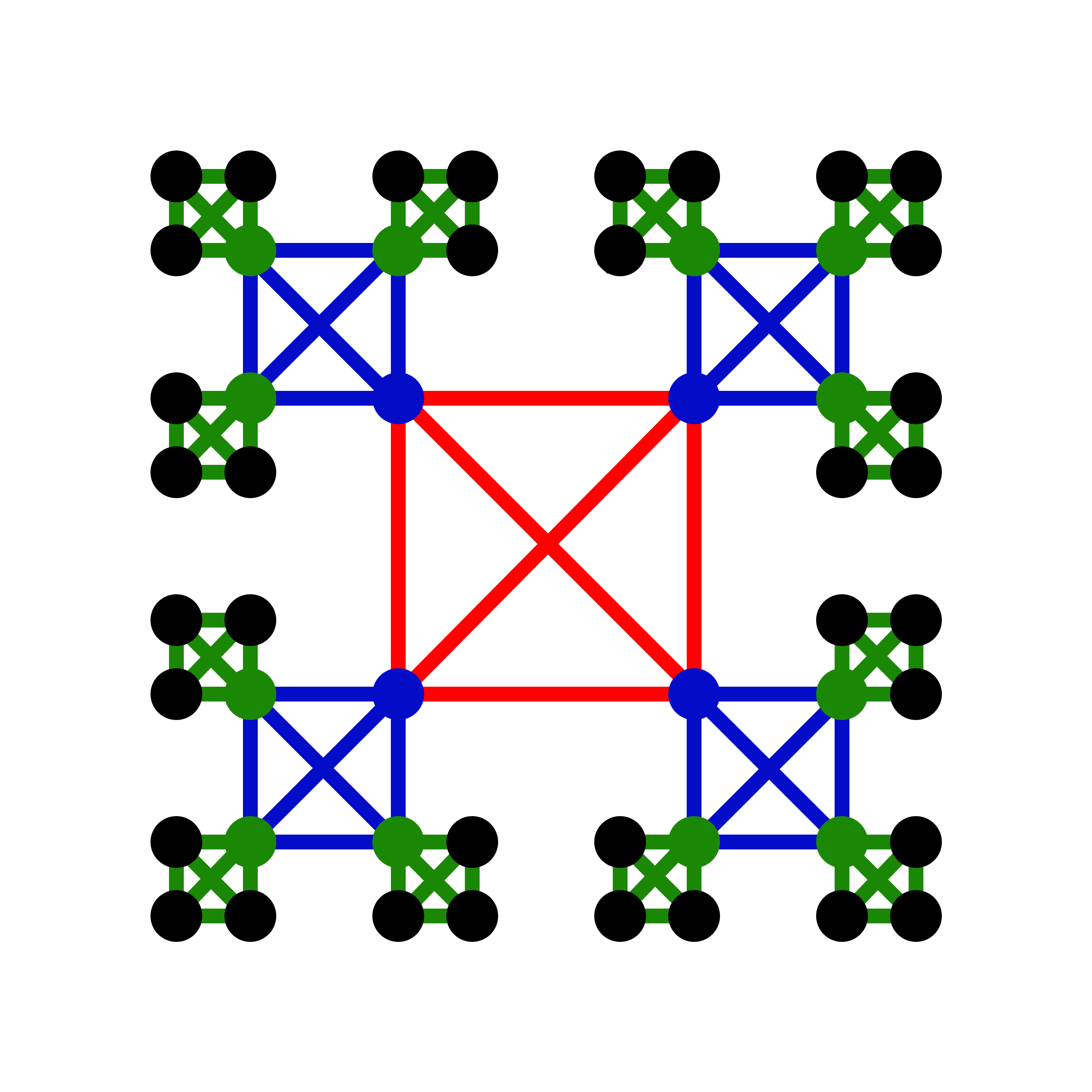
Figure 6: Diagram of the Husimi tree construction for three shells. The dots represent spins, and the boxes tetrahedra. Tetrahedra are a shown in a two-dimensional projection to highlight the tree’s topology. The outermost, zeroth shell of spins, is shown in black, the first in green, and the second in blue.

The Husimi tree approximation consists in replacing the pyrochlore lattice with a tree structure having the same local coordination but lacking any closed loops beyond those contained in single tetrahedra. This is illustrated in Fig. 6.

The Husimi tree of depth $L$ can be seen as being composed of $L+1$ shells of spins, which we label by an integer $n$. We label the outermost shell as $n=0$ and the innermost as $n=L$. The outermost tetrahedra are composed of three spins from shell $n=0$ and one from shell $n=1$. Moving inwards, tetrahedra are then composed of three spins from shell $n=m$ and one from shell $n=m+1$, until the central tetrahedron which is composed of four spins from shell $n=L$.

The partition function, and thermodynamic expectation values of quantities on the tree can be built up by successively summing over the states of each shell, working from outermost to innermost. Quantities such as the energy and magnetisation are calculated by finding their average value on the central tetrahedron, which we take as being representative of a tetrahedron in the bulk of the pyrochlore lattice. This approach has already been shown to be quite successful in describing spin ice Jaubert et al. (2008); Jaubert (2009); Jaubert et al. (2013); Otsuka et al. (2018) and related Ising models Jurčišinová and Jurčišin (2017).

We once again consider an external field ${\bf h}$ with the largest Cartesian component along the $z$-direction (i.e. $\cos(\theta)>|\sin(\theta)\sin(\varphi)|,|\sin(\theta)\cos(\varphi)|$. Other cases can be simply obtained by applying cubic lattice symmetries to this case.

To somewhat simplify our expressions, we will take the energy of the ground state to be zero, and then reintroduce the original ground state Zeeman energy after the recursion relation has been solved. The original Zeeman energy per spin in the ground state is:

$$u_{0}=-\frac{h}{\sqrt{3}}\cos(\theta)$$ (24)

Furthermore, we introduce new Ising variables $\tau_{i}$ which take the value $+1$ if spin $\vec{S}_{i}$ has a positive projection along $\vec{h}$ and $-1$ otherwise. $\tau_{i}$ relate to the $\sigma_{i}$ introduced in Eq. (3) via:

$$\tau_{i}=\epsilon_{i}\sigma_{i}$$ (25)

with $\epsilon_{i}=(1,-1,-1,1)$ respectively for sublattices $1-4$ (cf. Eq. (2)).

In calculating the partition function, $Z$, we only include configurations where the ice rule is obeyed everywhere, i.e.

$$\sum_{i\in t}\sigma_{i}=\sum_{i\in t}\epsilon_{i}\tau_{i}=0$$ (26)

for all tetrahedra, $t$.

The partition function of the Husimi tree is

$$Z=\sum_{\{\tau\}}e^{\sum_{j}\beta E_{j}(\tau_{j}-1)/2}\prod_{t}\left(\delta_{\sum_{i\in t}\epsilon_{i}\tau_{i},0}\right)$$ (27)

where $\sum_{\{\tau\}}$ is a sum over all configurations of the Ising variables $\tau_{j}$, $\prod_{t}$ is a product over all tetrahedra in the tree, the Kronecker delta $\delta_{\sum_{i\in t}\epsilon_{i}\tau_{i},0}$ enforces the ice rule on each tetrahedron and $E_{j}$ is the energy cost of flipping $\tau_{j}$ against the applied field.

$E_{j}=2\epsilon_{j}\vec{h}\cdot\hat{e}_{j}$ [cf. Eq. (2)] depends on which of the four sublattices $j$ belongs to. $E_{j}$ can therefore take four possible values which we label $E_{1},E_{2},E_{3},E_{4}$ with the subscript now corresponding to the sublattice label.

To make progress with Eq. (27) we consider it as sum of six terms, corresponding to the six possible arrangements of the central tetrahedron. Each term in the sum is then a product of the partition function of the four branches, taken with fixed values of the spins on layer $n=L$. This gives us:

$$Z=Z_{+1,1,L}Z_{+1,2,L}Z_{+1,3,L}Z_{+1,4,L}+$$

$$\exp(-\beta(E_{1}+E_{2}))Z_{-1,1,L}Z_{-1,2,L}Z_{+1,3,L}Z_{+1,4,L}+$$

$$\exp(-\beta(E_{1}+E_{3}))Z_{-1,1,L}Z_{+1,2,L}Z_{-1,3,L}Z_{+1,4,L}+$$

$$\exp(-\beta(E_{2}+E_{4}))Z_{+1,1,L}Z_{-1,2,L}Z_{+1,3,L}Z_{-1,4,L}+$$

$$\exp(-\beta(E_{3}+E_{4}))Z_{+1,1,L}Z_{+1,2,L}Z_{-1,3,L}Z_{-1,4,L}+$$

$$\exp(-\beta(E_{1}+E_{2}+E_{3}+E_{4}))Z_{-1,1,L}Z_{-1,2,L}Z_{-1,3,L}Z_{-1,4,L}.$$

(28)

where $Z_{\tau,i,n}$ is the partition function of a branch terminating on a site of sublattice $i$ at layer $n$, with the value of the terminating spin fixed to $\tau$.

$Z_{\tau,i,n}$ have a recursion relation:

$$Z_{\tau,i,n+1}=$$

$$\left(\prod_{j\neq i}\sum_{\tau_{j}=\pm 1}\right)\delta_{\epsilon_{i}\tau+\sum_{j\neq i}\epsilon_{j}\tau_{j},0}e^{\beta E_{j}(\tau_{j}-1)/2}\prod_{j\neq i}Z_{\tau_{j},j,n}.$$

(29)

To simplify the notation, we define:

$$A_{n}=Z_{+1,1,n},\ \ \alpha_{n}=Z_{-1,1,n}$$

$$B_{n}=Z_{+1,2,n},\ \ \beta_{n}=Z_{-1,2,n}$$

$$C_{n}=Z_{+1,3,n},\ \ \gamma_{n}=Z_{-1,3,n}$$

$$D_{n}=Z_{+1,4,n},\ \ \delta_{n}=Z_{-1,1,n}$$ (30)

These can be calculated easily for $n=1$ because this only requires summing over the configurations of three spins on the outermost layer (see Fig. 6). For example

$$A_{1}= 1+e^{-\beta(E_{3}+E_{4})}+e^{-\beta(E_{2}+E_{4})}$$ (31)

$$\alpha_{1}= e^{-\beta(E_{2}+E_{3}+E_{4})}+e^{-\beta E_{2}}+e^{-\beta E_{3}}.$$ (32)

The partition function of the full tree [Eq. (28)] can then be obtained by repeatedly applying the recursion relation Eq. (29) to calculate $Z_{\tau,i,L}$.

The sequence thus generated is, however, diverging for $L\to\infty$. Fortunately, useful thermodynamic quantities such as the internal energy and magnetisation can be expressed in terms of four new sequences, which all converge to a finite limit with increasing $L$. These four new sequences are:

$$Y_{n}=\frac{\alpha_{n}}{A_{n}}e^{-\beta E_{1}};\ X_{n}=\frac{\beta_{n}}{B_{n}}e^{-\beta E_{2}};\\ W_{n}=\frac{\gamma_{n}}{C_{n}}e^{-\beta E_{3}};\ V_{n}=\frac{\delta_{n}}{D_{n}}e^{-\beta E_{4}}$$ (33)

The recursion relations obeyed by these sequences are given in Appendix A.

To extract useful approximations for thermodynamic quantities for spin ice, we make the assumption that the central tetrahedron of the tree is representative of a tetrahedron in the bulk of the pyrochlore lattice, and that its mean magnetisation and internal energy are good approximations for the magnetisation and internal energy of spin ice per ‘A’ tetrahedron.

Using this approach, we use Eq. (24) to write down an expression for the internal Zeeman energy per spin as:

$$U=-\frac{h}{\sqrt{3}}\cos(\theta)+\frac{1}{4R_{L}}\bigg{(}(E_{1}+E_{3})Y_{L}W_{L}$$

$$\qquad+(E_{1}+E_{2})Y_{L}X_{L}+(E_{3}+E_{4})V_{L}W_{L}$$

$$\qquad+(E_{2}+E_{4})X_{L}V_{L}$$

$$\qquad+(E_{1}+E_{2}+E_{3}+E_{4})Y_{L}X_{L}W_{L}V_{L}\bigg{)}$$ (34)

where

$$R_{L}=1+Y_{L}W_{L}+Y_{L}X_{L}+V_{L}W_{L}+$$

$$\qquad\qquad X_{L}V_{L}+Y_{L}X_{L}W_{L}V_{L}.$$ (35)

IV.2 Heat Capacity and Entropy

To gain some initial insight into the dependence of the thermodynamic quantities on field direction, we consider the heat capacity, $C(T)$, and entropy, $S(T)$.

We calculate the heat capacity in our Husimi tree calculations by calculating the energy per spin according to Eq. (34), with $L=1000$ shells, at a series of temperatures, and then calculating the temperature derivative $C=\left(\frac{\partial U}{\partial T}\right)_{\vec{h}}$ numerically. The results of this are shown for a series of different field directions in Fig. 7.

Approaching $T_{K}$ from above, the heat capacity increases sharply, but does not diverge, implying an absence of latent heat at the transition. At $T_{K}$, the heat capacity drops discontinuously to zero, as a result of the complete absence of fluctuations for $T<T_{K}$. The value of $T_{K}$ found in the Husimi tree calculation agrees with the prediction of Eq. (10) for all field directions.

Rotating the field direction away from $[001]$ and towards the phase boundaries of Fig. 2, shifts $T_{K}$ to lower temperatures and decreases the size of the discontinuity in $C$. At the phase boundaries, the discontinuity disappears and $C$ exhibits only a smooth maximum.

The entropy change between two temperatures $T_{1}$ and $T_{2}$ is obtained from the integral of $C/T$:

$$\Delta S=\int_{T_{1}}^{T_{2}}\frac{C(T)}{T}dT.$$ (36)

For field directions for which a Kasteleyn transition occurs (i.e. those not lying on the phase boundaries of Fig. 2) we know that $S(T<T_{K})=0$, since all fluctuations are suppressed for $T<T_{K}$. For such field directions we can therefore obtain the absolute entropy per site by integrating up from $T_{K}$:

$$S(T)=\int_{T_{K}}^{T}\frac{C(T^{\prime})}{T^{\prime}}dT^{\prime}.$$ (37)

For large temperatures we find that this calculation recovers the Pauling entropy:

$$S_{\rm Pauling}=\frac{1}{2}\log\left(\frac{3}{2}\right)\approx 0.203$$ (38)

for all field directions not lying on the phase boundaries.

With this knowledge in hand we can then use the assumption that $S(T)$ is independent of field direction for $T\gg h$ to calculate the residual ($T=0$) entropy $S_{0}$ on the phase boundaries:

$$S_{0}=S_{\rm Pauling}-\int_{0}^{\infty}\frac{C(T^{\prime})}{T^{\prime}}dT^{\prime}.$$ (39)

We find that $S_{0}=0$ along the phase boundaries, apart from at the kagome ice points, which occur where three phases meet in Fig. 2. This is because the lines of phase boundary apart from the kagome ice points have only sub-extensive ground state degeneracy.

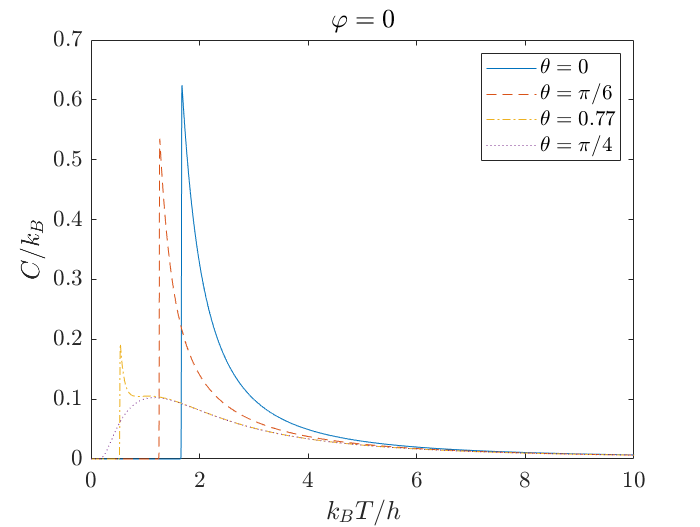
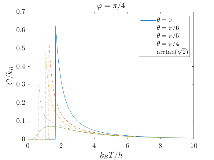
Figure 7: Heat capacity per spin as a function of temperature $C(T)$, using the Husimi tree approximation, for various values of $\theta$ with $\varphi=0$ [(a)] and $\varphi=\frac{\pi}{4}$ [(b)]. 1000 shells are used for the Husimi tree. The heat capacity is discontinuous, but not divergent, at the Kasteleyn transition, indicating that there is no latent heat associated with the transition. The discontinuity gets progressively smaller and moves to lower temperature as the field direction is tuned towards the phase boundaries of Fig. 2 before disappearing entirely at the boundaries.

At the kagome ice points we find

$$S_{0}\approx 0.072$$ (40)

in agreement with the modified Pauling estimate Udagawa et al. (2002) for kagome ice $S^{KI}_{\rm Pauling}=\frac{1}{4}\log\left(\frac{4}{3}\right)$. This differs by about $10\%$ from the exact result for the entropy of kagome ice Udagawa et al. (2002); Moessner and Sondhi (2001). The fact that we find agreement with the Pauling approximation, rather than the exact result, is a consequence of using the Husimi tree approximation.

With the $T\to 0$ limit of the entropy now determined for all parameter sets, we can calculate the absolute entropy for all temperatures and field directions. The results of this are shown in Fig. 8.

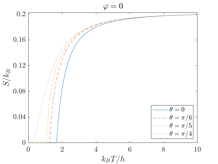
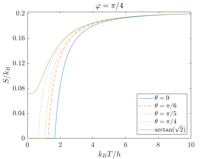
Figure 8: Entropy per spin as a function of temperature, $S(T)$, using the Husimi tree approximation, for various values of $\theta$ with $\varphi=0$ [(a)] and $\varphi=\frac{\pi}{4}$ [(b)]. 1000 shells are used in the Husimi tree in all cases. The entropy falls to zero at the Kasteleyn temperature, and remains at zero below the transition. For field directions corresponding to the $T=0$ phase boundaries in Fig. 2 ($\varphi=0,\theta=\frac{\pi}{4};\varphi=\frac{\pi}{4},\theta=\arctan(\sqrt{2})$), no Kasteleyn transition is seen. The ground state entropy is however vanishingly small for all these directions except the kagome ice point ($\varphi=\frac{\pi}{4},\theta=\arctan(\sqrt{2})$), where a limit of $0.072k_{B}$ is found.

IV.3 Magnetisation and Magnetic Torque

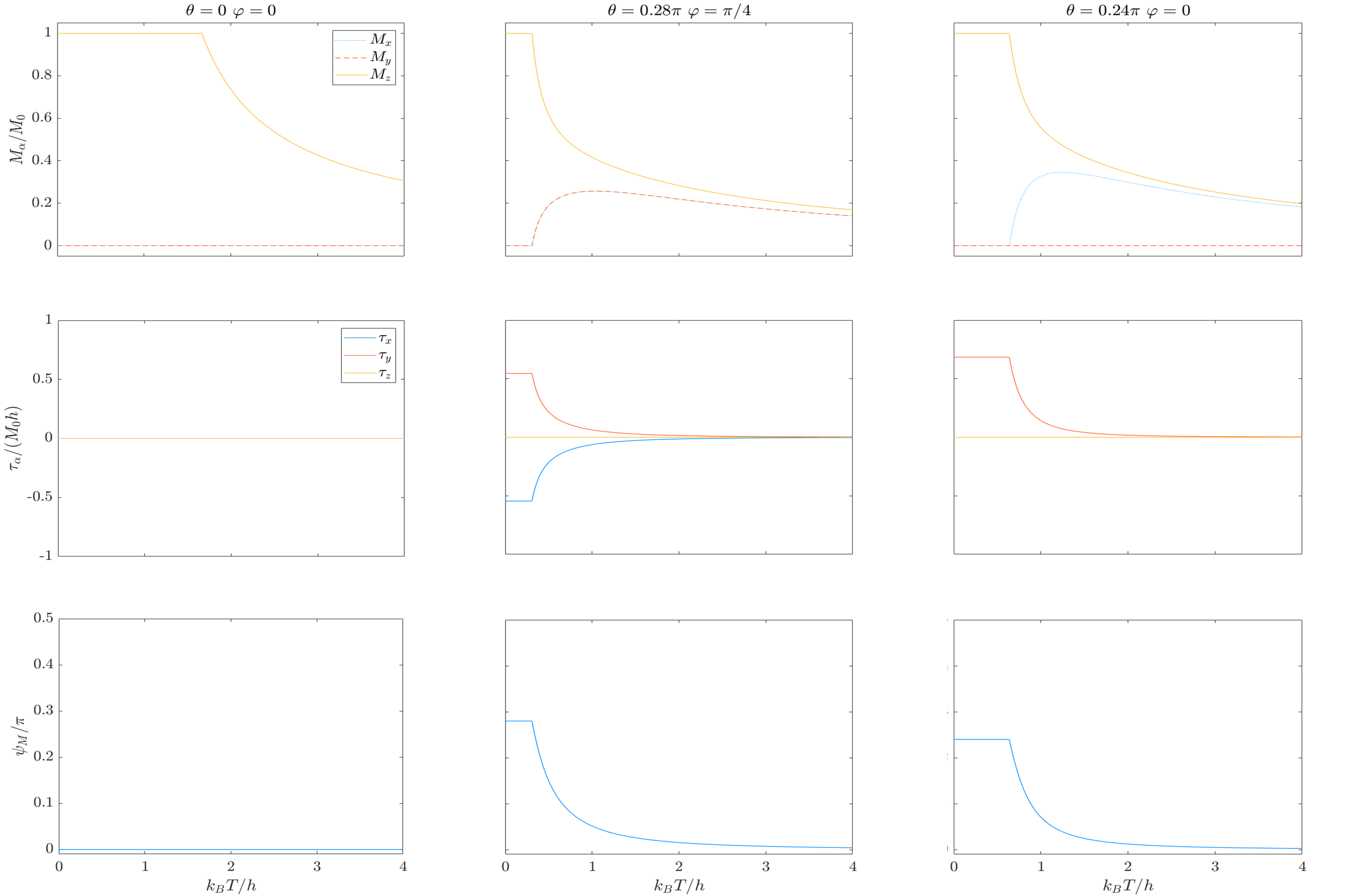
Figure 9: Magnetisation (top row), magnetic torque (middle row) and angle between magnetisation and applied field (bottom row) as a function of temperature for three different field directions. The three columns correspond to the three field directions: the [001] direction (left column), a slight deviation from the [111] direction (middle) and a slight deviation from the [110] direction (right). The magnetisation rises rapidly before reaching a plateau at $T=T_{K}$ for all field directions. At high temperatures the magnetisation aligns with the field, as dictated by linear response and the cubic symmetries of the lattice resulting in vanishing torque, $\vec{\tau}$, and angle, $\psi_{M}$. For fields not aligned with [001], the magnetisation vector rotates continuously away from the field direction as temperature decreases towards $T_{K}$ resulting in rapid rises in both $\vec{\tau}$ and $\psi_{M}$.

In this section we present calculations of the magnetisation and magnetic torque as a function of temperature.

Much like the internal energy, we take the mean magnetisation per four spins of spin ice to be the mean magnetisation of the central Husimi tree tetrahedron. This gives us the following expressions for the components of the magnetisation, presented as a fraction of the saturation magnetisation $M_{0}=\frac{N}{\sqrt{3}}$, with $N$ the total number of spins in the system:

$$\frac{M_{x}}{M_{0}}= \frac{X_{L}V_{L}-Y_{L}W_{L}}{R_{L}}$$ (41)

$$\frac{M_{y}}{M_{0}}= \frac{V_{L}W_{L}-Y_{L}X_{L}}{R_{L}}$$ (42)

$$\frac{M_{z}}{M_{0}}= \frac{1-Y_{L}X_{L}W_{L}V_{L}}{R_{L}}$$ (43)

where $R_{L}$ is defined by Eq. (35).

The torque acting on the system is found by taking the cross product between the magnetisation and the external field:

$$\vec{\tau}=\vec{M}\times\vec{h}.$$ (44)

We present the results for the torque in units of $M_{0}|\vec{h}|$, the value that would be obtained in an extreme limit where the system is polarized in a direction orthogonal to the field. We also present calculations for the angle between between the magnetisation and the field:

$$\psi_{M}=\arccos{\left(\frac{\vec{M}\cdot\vec{h}}{|\vec{M}||\vec{h}|}\right)}$$ (45)

The evolution of $\vec{M}$, $\vec{\tau}$ and $\psi_{M}$ are shown as a function of temperature for three different field directions in Fig. 9.

At high temperatures $T\gg h$, the magnetisation is determined by the linear response:

$$M_{\alpha}=\sum_{\beta}\chi_{\alpha\beta}h_{\beta}$$ (46)

and since the cubic symmetry of the lattice requires $\chi_{\alpha\beta}=\chi\delta_{\alpha\beta}$ we have ${\vec{M}}\parallel\vec{h}$. $\vec{\tau}$ and $\psi_{M}$ therefore vanish in the high temperature limit for all field directions, as seen in Fig. 9.

On the other hand, for $T<T_{K}$, ${\vec{M}}$ aligns along whichever $\langle 001\rangle$ axis makes the smallest angle with ${\vec{h}}$. For generic field directions, this angle may be significant, and a large magnetic torque is present in the ordered phase.

The evolution from ${\vec{M}}\parallel{\vec{h}}$ to ${\vec{M}}\parallel\langle 001\rangle$ happens via a continuous rotation of the magnetisation relative to the field as the system is cooled. This process accelerates as $T$ approaches $T_{K}$ from above. The central and right columns of Fig. 9 show this for two field directions, one close to the $[111]$ direction the other close to the $[101]$ direction. The value of the magnetic torque obtained as $T\to T_{K}$ is in both cases a significant fraction of the maximum possible value $M_{0}|\vec{h}|$, illustrating the strength of this effect.

The small misalignment from the $[111]$ and $[101]$ assumed in the calculations in Fig. 9 is important. If the field were exactly aligned with the high symmetry direction $\vec{\tau}$ and $\psi_{M}$ would vanish at all temperatures, by symmetry. The misalignment allows $\vec{\tau}$ and $\psi_{M}$ to appear without breaking symmetries, and also makes $T_{K}$ finite. The approach to $T_{K}$ is then associated with a rapid growth of $\vec{\tau}$ and $\psi_{M}$ as the magnetisation rotates towards a $\langle 001\rangle$ direction.

In this sense, the high symmetry alignments along $\langle 111\rangle$ and $\langle 110\rangle$ are unstable at low temperatures - small misalignments will produce a torque which makes the misalignment worse.

IV.4 Rotational Magnetocaloric Effect

As a final application of our theory, we present calculations of the Rotational Magnetocaloric Effect (RMCE).

As shown in Fig. 4, the Kasteleyn temperature $T_{K}$ depends sensitively on the direction of the applied field. The surface $T_{K}(\theta,\phi)$ can be seen as as surface of constant, vanishing, entropy $S=0$. This already suggests other constant entropy surfaces, close to $S=0$, will vary strongly with field direction, which in turn implies that an adiabatic (constant entropy) rotation of the crystal relative to the field can induce large temperature changes. This is the rotational magnetocaloric effect.

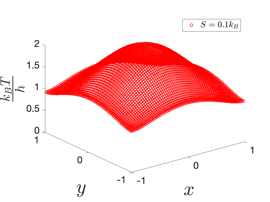
(a)

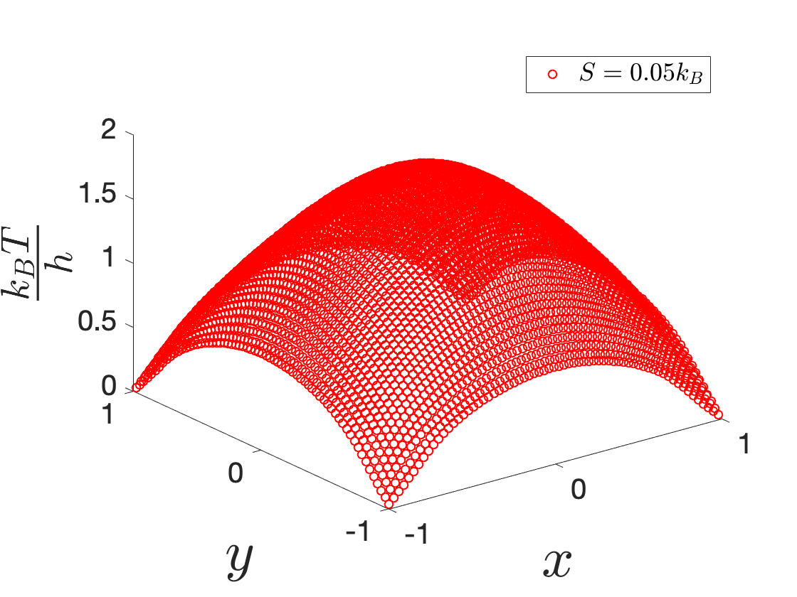
(b)

Figure 10: Temperature at constant entropy, as a function of field direction, for two values of the entropy per spin: $S=0.1k_{B}$ [(a)] and $S=0.05k_{B}$ [(b)]. At $S=0.1k_{B}$, adiabatically rotating the field away from the $[001]$ rotation, towards the $[101]$ or $[111]$ directions can reduce the temperature by a factor of $\sim 2$. For $S=0.05k_{B}$, much larger changes are possible, particularly by rotating towards the $[111]$ direction. If $S<S_{KI}$, the entropy of kagome ice, then within the idealized model studied here one can tune to arbitrarily low temperatures by rotating towards the $[111]$ direction, although this would not be true in a real system in which the degeneracy of kagome ice would not exact. The relationship between the coordinates $x,y$ and the field direction is given by Eqs. (6), (12)-(15).

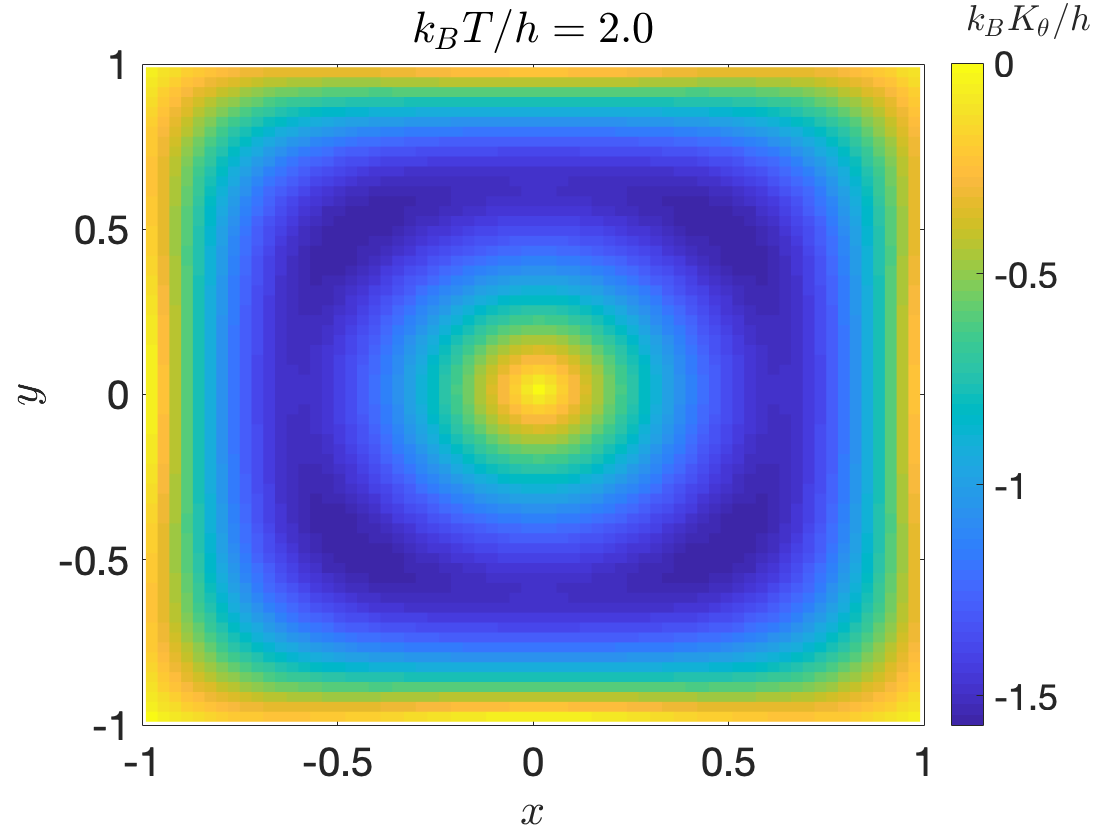
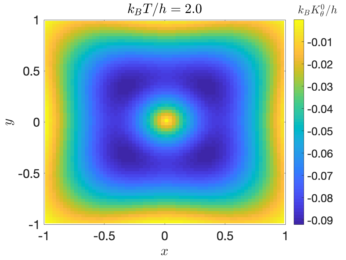
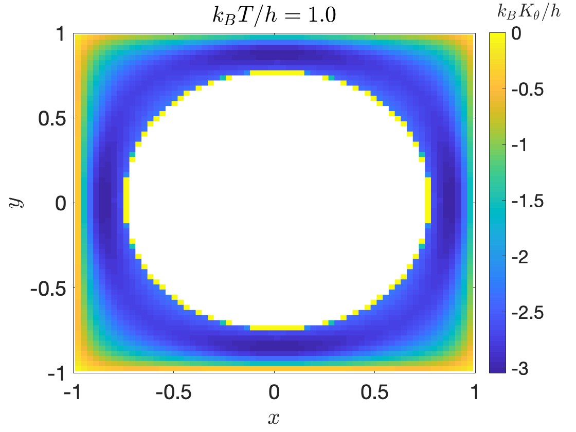
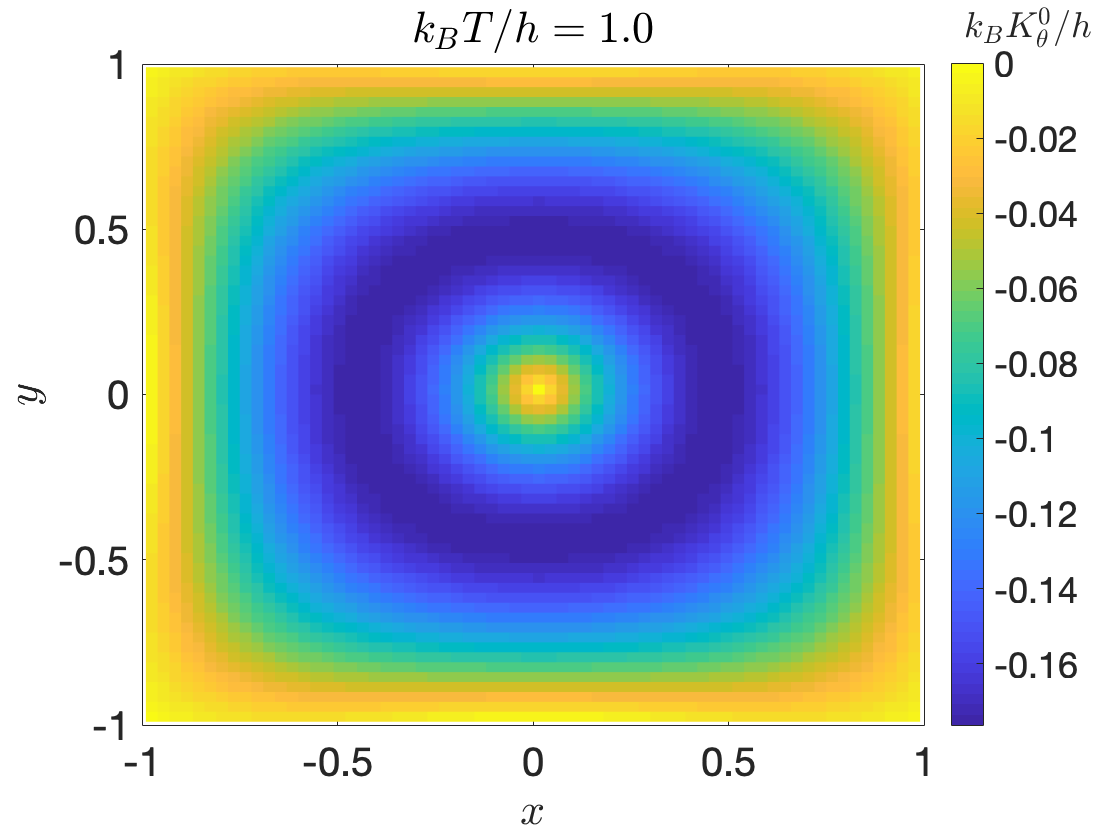
Figure 11: Angular cooling rate $K_{\theta}$ for spin ice (left column) and a system of non-interacting spins on the pyrochlore lattice with the same local anisotropy (right column). Results are shown for $k_{B}T=2h$ (top row) and $k_{B}T=h$ (bottom row). While the angular variation is similar between the interacting and non-interacting calculations, the overall magnitude of the cooling rate is an order of magnitude stronger for the interacting case. This demonstrates that the interactions encoded in the ice rule magnify the RMCE. The white region in the bottom left panel is in the field induced ordered phase $T<T_{K}$, in which case there is no RMCE. The relationship between the coordinates $x,y$ and the field direction is given by Eqs. (6), (12)-(15).

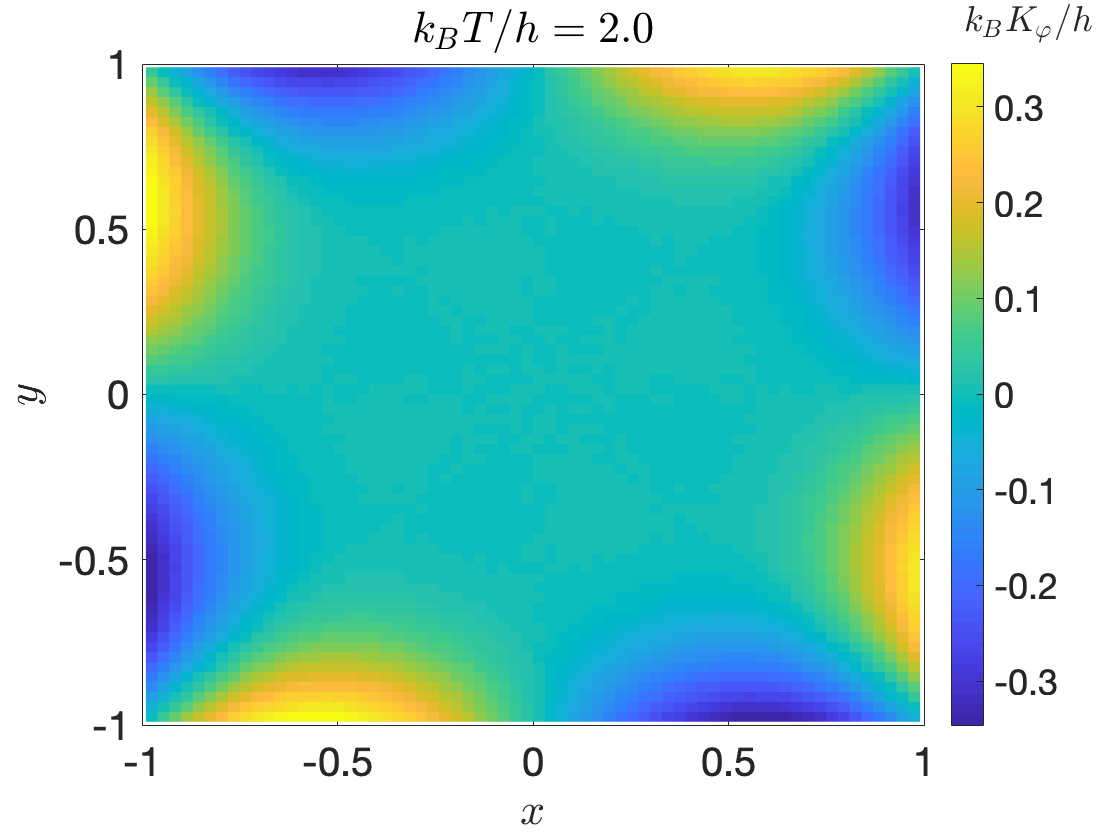
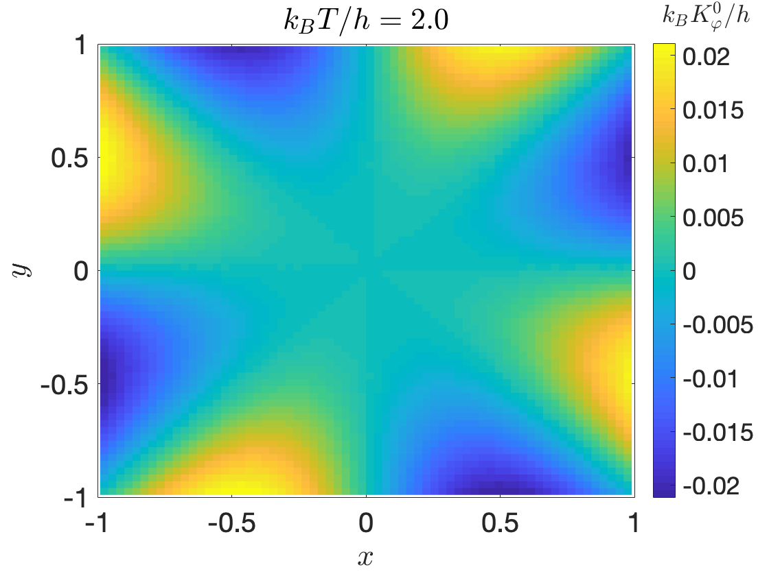
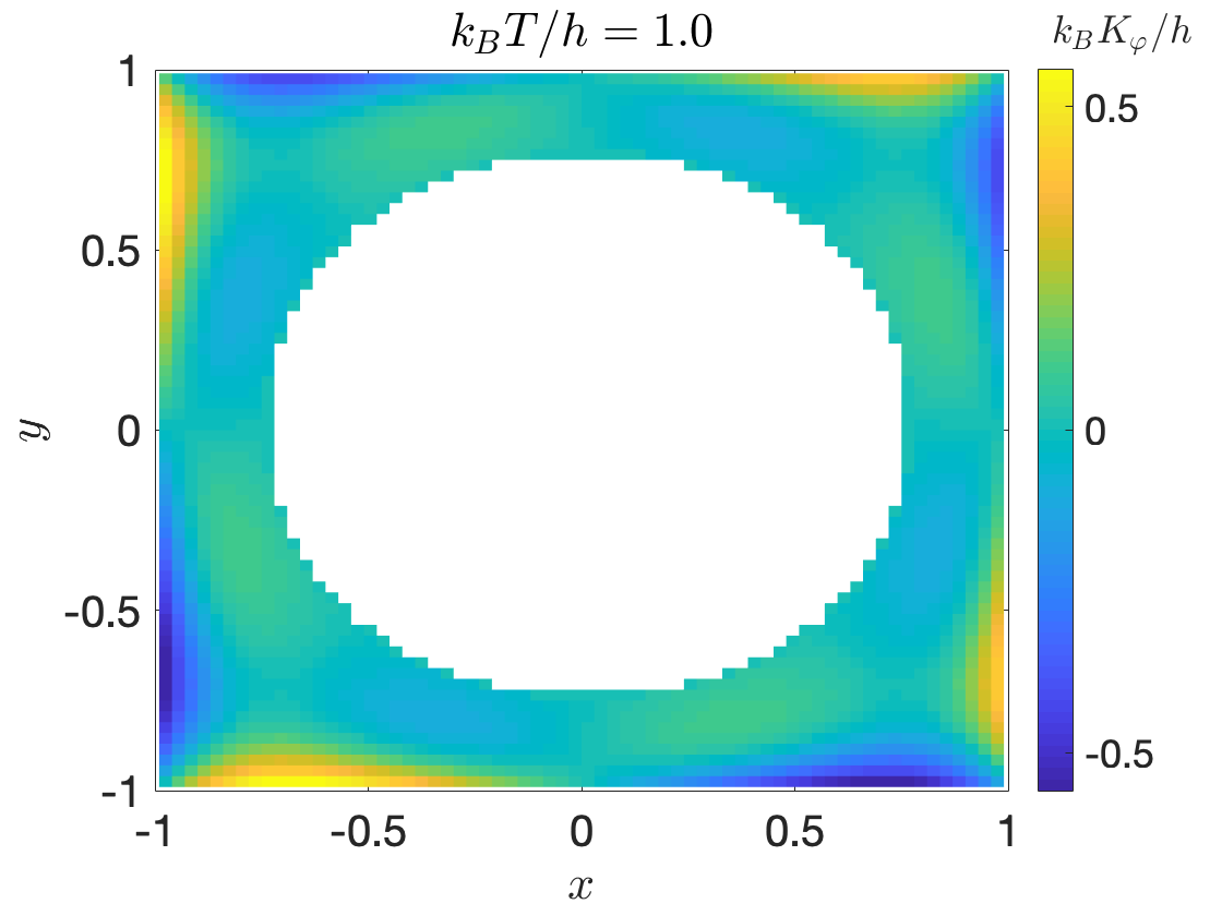
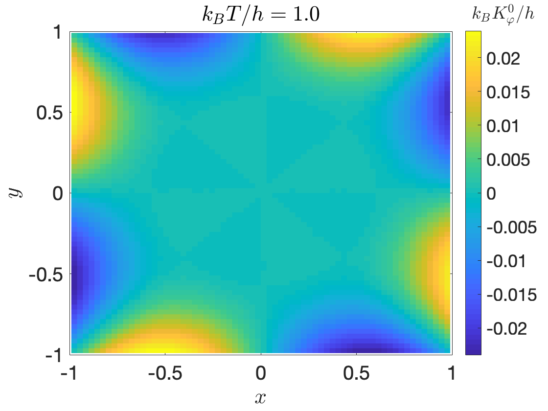
Figure 12: Angular cooling rate $K_{\varphi}$ for spin ice (left column) and a system of non-interacting spins on the pyrochlore lattice with the same local anisotropy (right column). Results are shown for $k_{B}T=2h$ (top row) and $k_{B}T=h$ (bottom row). The angular variation is similar between the interacting and non-interacting systems, but overall magnitude of the cooling rate is an order of magnitude stronger in the interacting case. $K_{\varphi}$ vanishes along the lines $x=\pm y,x=0,y=0$, in both interacting and non-interacting calculations which is a consequence of symmetry. The white region in the bottom left panel is in the field induced ordered phase $T<T_{K}$, in which case there is no RMCE. The relationship between the coordinates $x,y$ and the field direction is given by Eqs. (6), (12)-(15).

The variation of temperature with field direction at constant entropy is shown for two values entropy in Fig. 10. Adiabatic rotations which move the field away from the $[001]$ crystal direction reduce the temperature substantially. A temperature reduction by a factor of $\sim 2$ can be obtained at $S=0.1k_{B}$ and an even stronger cooling effect is obtained with lower entropies (lower starting temperature).

Entropies below that of kagome ice $S<S_{KI}$ allow cooling to arbitrarily low temperature, at the level of our idealized model, by rotating the field towards the $[111]$ crystal direction. This would be prevented in a real system by the presence of small perturbations to the Hamiltonian which lift the kagome ice degeneracy.

We define cooling rates for adiabatic rotation of the field direction as follows, with a negative cooling rate indicating a decrease in temperature for increasing angle:

$$K_{\theta}= \left(\frac{\partial T}{\partial\theta}\right)_{S}=\frac{-T}{C(T)}\left(\frac{\partial S}{\partial\theta}\right)_{T}$$ (47)

$$K_{\varphi}= \left(\frac{\partial T}{\partial\varphi}\right)_{S}=\frac{-T}{C(T)}\left(\frac{\partial S}{\partial\varphi}\right)_{T}$$ (48)

with $C(T)$ being the heat capacity calculated in Section IV.2. These relationships follow from the reciprocal relation for partial derivatives.

To provide a benchmark against which we can compare the RMCE in the spin ice model, we also calculate the cooling rates $K_{\theta}^{0}$ and $K_{\varphi}^{0}$ of a system of non-interacting spins on the pyrochlore lattice with the same local anisotropy. This benchmark system is described by a Hamiltonian

$$H_{0}=-\vec{h}\cdot\sum_{i}\vec{S}_{i}-D_{SI}\sum_{i}\left(\vec{S}_{i}\cdot\vec{e}_{i}\right)^{2}$$ (49)

with single-ion anisotropy $D_{SI}\to\infty$. This corresponds to Eq. (1) without the exchange interaction term, $J$. Thus by comparing $K_{\theta}$ and $K_{\varphi}$ to $K_{\theta}^{0}$ and $K_{\varphi}^{0}$ we can observe the effect of the interactions encoded in the ice rule on the RMCE. The calculation of the non-interacting cooling rates $K_{\theta}^{0}$ and $K_{\varphi}^{0}$ is described in Appendix B.

For both interacting and non-interacting systems the angular cooling rates decay as $\frac{1}{T}$ at high temperature. This follows from Eqs. (47) - (48), and the cubic symmetry of the system which causes the angular derivatives of entropy to vanish as $\frac{1}{T^{4}}$ at high temperature (see Appendix C).

The angular cooling rates for both interacting and non-interacting systems are shown in Figs. 11-12, for temperatures $k_{B}T=2h$ and $k_{B}T=h$. From the overall scale of the variation in Figs. 11-12 we see that the strong interactions in spin ice enhance the RMCE by roughly an order of magnitude at these intermediate temperatures. The azimuthal cooling rate $K_{\varphi}$ varies in sign, vanishing along the lines $\varphi=n\frac{\pi}{4},n\in\mathbb{Z}$, in both interacting and non-interacting calculations. This is a consequence of the cubic symmetry of the lattice.

V Summary and Conclusions

In this Article we have presented a theory of spin ice in the presence of an applied magnetic field with arbitrary orientation. We have shown that the Kasteleyn transition known for the case of a field oriented along $\langle 001\rangle$ appears for general field directions, and have calculated the dependence of the Kasteleyn temperature $T_{K}$ on field direction. We find that $T_{K}$ vanishes along certain special lines of field-orientation-space.

In real spin ices, the presence of a finite density of monopoles - neglected in our calculation turns the Kasteleyn transition from a sharp transition into a crossover. This crossover temperature can be extracted from magnetisation measurements Pili et al. and our predictions regarding the behaviour of $T_{K}$ as a function of field direction – in particular the singular behavior approaching the phase boundaries of Fig. 2 – could thus be tested.

We have further investigated the thermodynamics of the Coulomb phase for $T>T_{K}$ using a Husimi tree approximation, with an emphasis on those properties related to the anisotropic response of spin ice to a magnetic field. We find that fields oriented away from high-symmetry directions generate large magnetic torque as $T$ approaches $T_{K}$ from above. Moreover, the strong dependence of the entropy on field direction leads to a rotational magnetocaloric effect by which the system can be cooled or heated using adiabatic rotations of the crystal relative to the applied field. This effect is enhanced significantly above what would be expected for a non-interacting system with the same magnetic anisotropy.

Kittaka et al. have measured the RMCE in crystals of Dy₂Ti₂O₇ Kittaka et al. (2018). Our results cannot be directly compared with their’s, because their measurements were carried out in a field and temperature regime in which ice-rule violations (monopoles) are important, and these are absent from our description.

Our results provide a case study of enhanced RMCE in a frustrated system, and affirm the usefulness of RMCE as a probe of exotic physics in anisotropic magnets. It would be interesting to apply these ideas to putative quantum spin ices, particularly those with a multipolar nature such as the Pr- or Ce- based pyrochlores Onoda and Tanaka (2010); Petit et al. (2016); Sibille et al. (2018); Gaudet et al. (2019); Gao et al. (2019); Sibille et al. (2020); Smith et al. ; Bhardwaj et al. , in which RMCE could provide an alternative way of constraining the frustrated multipolar interactions.

Appendix A Recursion relations used in Husimi tree calculation

In this Appendix we present the recursion relations used in the Husimi tree calculations of Section IV.

The 8 sequences of partition functions in Eq. (30) obey the following recursion relations:

$$A_{n+1}=B_{n}C_{n}D_{n}+B_{n}\gamma_{n}\delta_{n}e^{-\beta(E_{3}+E_{4})}\\ +\beta_{n}C_{n}\delta_{n}e^{-\beta(E_{2}+E_{4})}$$ (50)

$$\alpha_{n+1}=\beta_{n}\gamma_{n}\delta_{n}e^{-\beta(E_{2}+E_{3}+E_{4})}+\beta_{n}C_{n}D_{n}e^{-\beta(E_{2})}\\ +B_{n}\gamma_{n}D_{n}e^{-\beta(E_{3})}$$ (51)

$$B_{n+1}=A_{n}D_{n}C_{n}+\alpha_{n}D_{n}\gamma_{n}e^{-\beta(E_{1}+E_{3})}\\ +A_{n}\delta_{n}\gamma_{n}e^{-\beta(E_{4}+E_{3})}$$ (52)

$$\beta_{n+1}=\alpha_{n}\delta_{n}\gamma_{n}e^{-\beta(E_{1}+E_{4}+E_{3})}+\alpha_{n}D_{n}C_{n}e^{-\beta(E_{1})}\\ +A_{n}\delta_{n}C_{n}e^{-\beta(E_{4})}$$ (53)

$$C_{n+1}=D_{n}A_{n}B_{n}+D_{n}\alpha_{n}\beta_{n}e^{-\beta(E_{2}+E_{1})}\\ +\delta_{n}A_{n}\beta_{n}e^{-\beta(E_{4}+E_{2})}$$ (54)

$$\gamma_{n+1}=\delta_{n}\alpha_{n}\beta_{n}e^{-\beta(E_{4}+E_{1}+E_{2})}+D_{n}\alpha_{n}B_{n}e^{-\beta(E_{1})}\\ +\delta_{n}A_{n}B_{n}e^{-\beta(E_{4})}$$ (55)

$$D_{n+1}=C_{n}B_{n}A_{n}+\gamma_{n}B_{n}\alpha_{n}e^{-\beta(E_{3}+E_{1})}\\ +C_{n}\beta_{n}\alpha_{n}e^{-\beta(E_{2}+E_{1})}$$ (56)

$$\delta_{n+1}=\gamma_{n}\beta_{n}\alpha_{n}e^{-\beta(E_{3}+E_{2}+E_{1})}+C_{n}\beta_{n}A_{n}e^{-\beta(E_{2})}\\ +\gamma_{n}B_{n}A_{n}e^{-\beta(E_{3})}$$ (57)

The series generated by the recursion relations (50)-(57) does not converge as $L\to\infty$. However, physical quantities can be written in terms of the variables $Y_{n}$,$X_{n}$, $W_{n}$, $V_{n}$ for which the corresponding series do converge. The recursion relations for these variables are:

$$Y_{n+1}=e^{-\beta E_{1}}\frac{X_{n}W_{n}V_{n}+X_{n}+W_{n}}{1+V_{n}W_{n}+X_{n}V_{n}};\ Y_{0}=e^{-\beta E_{1}}$$ (58)

$$X_{n+1}=e^{-\beta E_{2}}\frac{W_{n}Y_{n}V_{n}+Y_{n}+V_{n}}{1+Y_{n}W_{n}+V_{n}W_{n}};\ V_{0}=e^{-\beta E_{2}}$$ (59)

$$W_{n+1}=e^{-\beta E_{3}}\frac{V_{n}Y_{n}X_{n}+Y_{n}+V_{n}}{1+Y_{n}X_{n}+X_{n}V_{n}};\ W_{0}=e^{-\beta E_{3}}$$ (60)

$$V_{n+1}=e^{-\beta E_{4}}\frac{W_{n}X_{n}Y_{n}+X_{n}+W_{n}}{1+Y_{n}W_{n}+Y_{n}X_{n}};\ V_{0}=e^{-\beta E_{4}}$$ (61)

Appendix B Details of uncoupled spins calculation

We here present details of how the cooling rates $C_{r,\theta}^{0}$ and $C_{r,\varphi}^{0}$, pertaining to a system of uncoupled spins with the same local anisotropy as spin ice, were calculated. In this model, the ice rule need not be obeyed, and we consider only the single-ion anisotropy and Zeeman terms of Eq. (1). We continue to assume that $D_{SI}\gg|\vec{h}|$ such the spins remain Ising-like and oriented along their local $\langle 111\rangle$ axis. Since the model is now non-interacting, the total entropy can be written as a sum of single-site entropies $S=\sum_{i}S_{i}$.

Starting with the ground state configuration of the interacting spin-ice model for an applied [001] field, we define energies $\Delta_{i}$ as the difference in Zeeman energy between the two possible orientations of the spin:

$$\Delta_{i}=2\vec{h}\cdot\vec{e}_{i}$$ (62)

with the local axes $\vec{e}_{i}$ defined for each sublattice in Eq. (2).

For each sublattice $i$, we can write down a single spin partition function as:

$$Z_{i}=e^{-\frac{\beta\Delta_{i}}{2}}+e^{\frac{\beta\Delta_{i}}{2}}=2\cosh\left(\frac{\beta\Delta_{i}}{2}\right)$$ (63)

The internal energy can be calculated straightforwardly as:

$$U_{i}=-\frac{\partial\log(Z_{i})}{\partial\beta}=-\frac{\Delta_{i}}{2}\tanh\left(\frac{\beta\Delta_{i}}{2}\right)$$ (64)

and the single spin entropy is

$$S_{i}=\log\left(2\cosh\left(\frac{\beta\Delta_{i}}{2}\right)\right)+\beta U_{i}$$ (65)

To calculate the cooling rate, we need the heat capacity, which we find by differentiating Eq. (64) with respect to $T$ at constant field:

$$C_{i}=\frac{\partial U}{\partial T}=\left(\frac{\beta\Delta_{i}}{2}\right)^{2}\operatorname{sech}^{2}\left(\frac{\beta\Delta_{i}}{2}\right)$$ (66)

The total heat capacity and entropy per spin are then $C=\frac{1}{4}\sum_{i=1}^{4}C_{i};S_{i}=\frac{1}{4}\sum_{i=1}^{4}S_{i}$ with the sums running over the four sublattices.

The rate of entropy change per site with respect to angle is then:

$$\frac{\partial S}{\partial\theta}=\frac{1}{4}\sum_{i=1}^{4}\frac{\partial\Delta_{i}}{\partial\theta}\frac{\partial S_{i}}{\partial\Delta_{i}}$$ (67)

$$\frac{\partial S}{\partial\phi}=\frac{1}{4}\sum_{i=1}^{4}\frac{\partial\Delta_{i}}{\partial\phi}\frac{\partial S_{i}}{\partial\Delta_{i}}$$ (68)

Where the derivatives of $\Delta_{i}$ with respect to angle follow from Eqs. (62) and (6):

$$\frac{\partial\Delta_{i}}{\partial\theta}=2h\left(\cos(\theta)\cos(\phi)\vec{e}_{i}^{\ x}+\cos(\theta)\sin(\phi)\vec{e}_{i}^{\ y}-\sin(\theta)\vec{e}_{i}^{\ z}\right)$$

(69)

$$\frac{\partial\Delta_{i}}{\partial\phi}=2h\left(-\sin(\theta)\sin(\phi)\vec{e}_{i}^{\ x}+\sin(\theta)\cos(\phi)\vec{e}_{i}^{\ y}\right)$$

and

$$\frac{\partial S_{i}}{\partial\Delta_{i}}=-\frac{1}{4}\beta^{2}\Delta_{i}\operatorname{sech}\left(\frac{\beta\Delta_{i}}{2}\right)^{2}.$$ (71)

Appendix C High temperature limit of angular derivatives of entropy

Here we showing that the high temperature limit of the angular derivatives of entropy $\frac{\partial S}{\partial\phi}$, $\frac{\partial S}{\partial\theta}$ behave as $\frac{1}{T^{4}}$ in the high temperature limit. This follows from the cubic symmetry of the problem.

We start by writing down a series expansion for $S(\beta)$, with $\beta=1/T$, around $\beta=0$

$$S(\beta)=\sum_{n=0}^{\infty}s_{n}\beta^{n}.$$ (72)

The magnetic field provides the only energy scale in the problem for both the case of spin ice and the non-interacting paramagnet (since we take, $J,D_{SI}\to\infty$. This means that $S(\beta)$ must be invariant under the rescaling $\beta\to\beta/\kappa;h\to\kappa h$, and so the coefficients $s_{n}$ must each scale as $h^{n}$ with $h$ being the magnitude of $\vec{h}=(h_{x},h_{y},h_{z})$.

Furthermore, the cubic symmetry of the system implies that each coefficient must be invariant under the action of the symmetry group $O_{h}$ applied to $\vec{h}$. Thus, the only symmetry allowed forms for the first few terms of Eq. (72) are

$$s_{0}=a;\ s_{1}=0;\ s_{2}=b(h_{x}^{2}+h_{y}^{2}+h_{z}^{2});\ s_{3}=0$$

$$s_{4}=c(h_{x}^{2}+h_{y}^{2}+h_{z}^{2})^{2}+d(h_{x}^{4}+h_{y}^{4}+h_{z}^{4})$$ (73)

with $a,b,c,d$ being field and temperature independent constants. Of the coefficients in Eq. (73), only $s_{4}$ depends on the field orientation and so the leading $\beta$ dependence of $\frac{\partial S}{\partial\phi}$, $\frac{\partial S}{\partial\theta}$ must be $\propto\beta^{4}$.

This argument holds both for the calculations for spin ice in the main text and for the calculations for non-interacting spins on the pyrochlore lattice in Appendix B.

It can readily be verified that if we expand Eq. (71) for small $\beta$ and insert the expansion into Eqs. (67)-(68), the $\beta^{2}$ terms cancel and the leading $\beta$ dependence is indeed $\sim\beta^{4}$.

Inserting this dependence into Eqs. (47)-(48) and using the fact that heat capacity $C\sim\frac{1}{T^{2}}$ at high temperature, we find that the angular cooling rates behave as $\sim\frac{1}{T}$.

References

- Harris et al. (1997) M. J. Harris, S. T. Bramwell, D. F. McMorrow, T. Zeiske, and K. W. Godfrey, Phys. Rev. Lett. 79, 2554 (1997).
- Balents (2010) L. Balents, Nature (London) 464, 199 (2010).
- Henley (2010) C. L. Henley, Annual Review of Condensed Matter Physics 1, 179 (2010).
- Castelnovo et al. (2012) C. Castelnovo, R. Moessner, and S. Sondhi, Annual Review of Condensed Matter Physics 3, 35 (2012).
- Ramirez et al. (1999) A. P. Ramirez, A. Hayashi, R. J. Cava, R. Siddharthan, and B. S. Shastry, Nature 399, 333 (1999).
- Melko and Gingras (2004) R. Melko and M. J. P. Gingras, J. Phys. Cond. Matt. 16, R1277 (2004).
- Isakov et al. (2005) S. V. Isakov, R. Moessner, and S. L. Sondhi, Phys. Rev. Lett. 95, 217201 (2005).
- Giblin et al. (2018) S. R. Giblin, M. Twengström, L. Bovo, M. Ruminy, M. Bartkowiak, P. Manuel, J. C. Andresen, D. Prabhakaran, G. Balakrishnan, E. Pomjakushina, C. Paulsen, E. Lhotel, L. Keller, M. Frontzek, S. C. Capelli, O. Zaharko, P. A. McClarty, S. T. Bramwell, P. Henelius, and T. Fennell, Phys. Rev. Lett. 121, 067202 (2018).
- Bramwell et al. (2001) S. T. Bramwell, M. J. Harris, B. C. den Hertog, M. J. P. Gingras, J. S. Gardner, D. F. McMorrow, A. R. Wildes, A. L. Cornelius, J. D. M. Champion, R. G. Melko, and T. Fennell, Phys. Rev. Lett. 87, 047205 (2001).
- Isakov et al. (2004a) S. V. Isakov, K. Gregor, R. Moessner, and S. L. Sondhi, Phys. Rev. Lett. 93, 167204 (2004a).
- Yavors’kii et al. (2008) T. Yavors’kii, T. Fennell, M. J. P. Gingras, and S. T. Bramwell, Phys. Rev. Lett. 101, 037204 (2008).
- Fennell et al. (2009) T. Fennell, P. P. Deen, A. R. Wildes, K. Schmalzl, D. Prabakharan, A. T. Boothroyd, R. J. Aldus, D. F. McMorrow, and S. T. Bramwell, Science 326, 415 (2009).
- Kanada et al. (2002) M. Kanada, Y. Yasui, Y. Kondo, S. Iikubo, H. Ito, M.and Harashina, M. Sato, H. Okumura, K. Kakurai, and H. Kadowaki, J. Phys. Soc. Jpn. 71, 313 (2002).
- Castelnovo et al. (2008) C. Castelnovo, R. Moessner, and S. L. Sondhi, Nature 451, 42 (2008).
- Morris et al. (2009) D. J. P. Morris, D. A. Tennant, S. A. Grigera, B. Klemke, C. Castelnovo, R. Moessner, C. Czternasty, M. Meissner, K. C. Rule, J.-U. Hoffmann, K. Kiefer, S. Gerischer, D. Slobinsky, and R. S. Perry, Science 326, 411 (2009).
- Jaubert and Holdsworth (2009) L. D. C. Jaubert and P. C. W. Holdsworth, Nature Physics 5, 258 (2009).
- Kadowaki et al. (2009) H. Kadowaki, N. Doi, Y. Aoki, Y. Tabata, T. J. Sato, J. W. Lynn, K. Matsuhira, and Z. Hiroi, J. Phys. Soc. Jpn. 78, 103706 (2009).
- Ryzhkin et al. (2013) M. I. Ryzhkin, I. A. Ryzhkin, and S. T. Bramwell, EPL 104, 37005 (2013).
- Kaiser et al. (2018) V. Kaiser, J. Bloxsom, L. Bovo, S. T. Bramwell, P. C. W. Holdsworth, and R. Moessner, Phys. Rev. B 98, 144413 (2018).
- Dusad et al. (2019) R. Dusad, F. K. K. Kirschner, J. C. Hoke, B. R. Roberts, A. Eyal, F. Flicker, G. M. Luke, S. J. Blundell, and J. C. Séamus Davis, Nature 517, 234 (2019).
- Samarakoon et al. (2022) A. M. Samarakoon, S. A. Grigera, D. A. Tennant, A. Kirste, B. Klemke, P. Strehlow, M. Meissner, J. N. Hallén, L. Jaubert, C. Castelnovo, and R. Moessner, Proceedings of the National Academy of Sciences 119 (2022).
- Fukazawa et al. (2002) H. Fukazawa, R. G. Melko, R. Higashinaka, Y. Maeno, and M. J. P. Gingras, Phys. Rev. B 65, 054410 (2002).
- Bramwell and Harris (1998) S. T. Bramwell and M. J. Harris, J. Phys. Cond. Matt. 10, L215 (1998).
- Moessner (1998) R. Moessner, Phys. Rev. B 57, R5587 (1998).
- Moessner and Sondhi (2003) R. Moessner and S. L. Sondhi, Phys. Rev. B 68, 064411 (2003).
- Hiroi et al. (2003a) Z. Hiroi, K. Matsuhira, S. Takagi, T. Tayama, and T. Sakakibara, J. Phys. Soc. Jpn. 72, 411 (2003a).
- Sakakibara et al. (2003) T. Sakakibara, T. Tayama, Z. Hiroi, K. Matsuhira, and S. Takagi, Phys. Rev. Lett. 90, 207205 (2003).
- Isakov et al. (2004b) S. V. Isakov, K. S. Raman, R. Moessner, and S. L. Sondhi, Phys. Rev. B 70, 104418 (2004b).
- Hiroi et al. (2003b) Z. Hiroi, K. Matsuhira, and M. Ogata, J. Phys. Soc. Jpn. 72, 3045 (2003b).
- Clancy et al. (2009) J. P. Clancy, J. P. C. Ruff, S. R. Dunsiger, Y. Zhao, H. A. Dabkowska, J. S. Gardner, Y. Qiu, J. R. D. Copley, T. Jenkins, and B. D. Gaulin, Phys. Rev. B 79, 014408 (2009).
- Guruciaga et al. (2016) P. C. Guruciaga, M. Tarzia, M. V. Ferreyra, L. F. Cugliandolo, S. A. Grigera, and R. A. Borzi, Phys. Rev. Lett. 117, 167203 (2016).
- Placke et al. (2020) B. Placke, R. Moessner, and O. Benton, Phys. Rev. B 102, 245102 (2020).
- Powell and Chalker (2008) S. Powell and J. T. Chalker, Phys. Rev. B 78, 024422 (2008).
- Jaubert et al. (2008) L. D. C. Jaubert, J. T. Chalker, P. C. W. Holdsworth, and R. Moessner, Phys. Rev. Lett. 100, 067207 (2008).
- Jaubert et al. (2009) L. D. C. Jaubert, J. T. Chalker, P. C. W. Holdsworth, and R. Moessner, J. Phys. Conf. Ser. 145, 012024 (2009).
- Harris et al. (1998) M. J. Harris, S. T. Bramwell, P. C. W. Holdsworth, and J. D. M. Champion, Phys. Rev. Lett. 81, 4496 (1998).
- (37) L. Pili, A. Steppke, M. E. Barber, F. Jerzembeck, C. W. Hicks, P. C. Guruciaga, D. Prabhakaran, R. Moessner, A. P. Mackenzie, S. A. Grigera, and R. A. Borzi, arXiv:2105.07977 .
- Baez and Borzi (2016) M. L. Baez and R. A. Borzi, Journal of Physics: Condensed Matter 29, 055806 (2016).
- Fennell et al. (2007) T. Fennell, S. T. Bramwell, D. F. McMorrow, P. Manuel, and A. R. Wildes, Nature Physics 3, 566 (2007).
- Zhitomirsky (2003) M. E. Zhitomirsky, Phys. Rev. B 67, 104421 (2003).
- Kohama et al. (2012) Y. Kohama, S. Wang, A. Uchida, K. Prsa, S. Zvyagin, Y. Skourski, R. D. McDonald, L. Balicas, H. M. Ronnow, C. Rüegg, and M. Jaime, Phys. Rev. Lett. 109, 167204 (2012).
- Tokiwa et al. (2013) Y. Tokiwa, M. Garst, P. Gegenwart, S. L. Bud’ko, and P. C. Canfield, Phys. Rev. Lett. 111, 116401 (2013).
- Manni et al. (2014) S. Manni, Y. Tokiwa, and P. Gegenwart, Phys. Rev. B 89, 241102 (2014).
- Aoki et al. (2004) H. Aoki, T. Sakakibara, K. Matsuhira, and Z. Hiroi, J. Phys. Soc. Jpn. 73, 2851 (2004).
- Orendáč et al. (2007) M. Orendáč, J. Hanko, E. Čižmár, A. Orendáčová, M. Shirai, and S. T. Bramwell, Phys. Rev. B 75, 104425 (2007).
- Pecharsky and Gschneidner (1997) V. K. Pecharsky and K. A. Gschneidner, Jr., Phys. Rev. Lett. 78, 4494 (1997).
- Gschneidner and Pecharsky (2008) K. Gschneidner and V. Pecharsky, International Journal of Refrigeration 31, 945 (2008).
- Balli et al. (2017) M. Balli, S. Jandl, P. Fournier, and A. Kedous-Lebouc, App. Phys. Rev. 4, 021305 (2017).
- Balli et al. (2014) M. Balli, S. Jandl, P. Fournier, and M. M. Gospodinov, App. Phys. Lett. 104, 232402 (2014).
- Kittaka et al. (2018) S. Kittaka, S. Nakamura, H. Kadowaki, H. Takatsu, and T. Sakakibara, Journal of the Physical Society of Japan 87, 073601 (2018).
- Kittaka et al. (2021) S. Kittaka, Y. Kono, S. Tsuda, T. Takabatake, and T. Sakakibara, Journal of the Physical Society of Japan 90, 064703 (2021).
- Udagawa et al. (2002) M. Udagawa, M. Ogata, and Z. Hiroi, J. Phys. Soc. Jpn. 71, 2365 (2002).
- Jaubert (2009) L. D. C. Jaubert, Topological constraints and defects in spin ice, Ph.D. thesis, Ecole Normale Supérieure de Lyon (2009).
- Jaubert et al. (2013) L. D. C. Jaubert, M. J. Harris, T. Fennell, R. G. Melko, S. T. Bramwell, and P. C. W. Holdsworth, Phys. Rev. X 3, 011014 (2013).
- Otsuka et al. (2018) H. Otsuka, Y. Okabe, and K. Nefedev, Phys. Rev. E 97, 042132 (2018).
- Jurčišinová and Jurčišin (2017) E. Jurčišinová and M. Jurčišin, Phys. Rev. E 96, 052128 (2017).
- Moessner and Sondhi (2001) R. Moessner and S. L. Sondhi, Phys. Rev. B 63, 224401 (2001).
- Onoda and Tanaka (2010) S. Onoda and Y. Tanaka, Phys. Rev. Lett. 105, 047201 (2010).
- Petit et al. (2016) S. Petit, E. Lhotel, S. Guitteny, O. Florea, J. Robert, P. Bonville, I. Mirebeau, J. Ollivier, H. Mutka, E. Ressouche, C. Decorse, M. Ciomaga Hatnean, and G. Balakrishnan, Phys. Rev. B 94, 165153 (2016).
- Sibille et al. (2018) R. Sibille, N. Gauthier, H. Yan, M. Ciomaga Hatnean, J. Ollivier, B. Winn, U. Filges, G. Balakrishnan, M. Kenzelmann, N. Shannon, and T. Fennell, Nature Physics 14, 711 (2018).
- Gaudet et al. (2019) J. Gaudet, E. M. Smith, J. Dudemaine, J. Beare, C. R. C. Buhariwalla, N. P. Butch, M. B. Stone, A. I. Kolesnikov, G. Xu, D. R. Yahne, K. A. Ross, C. A. Marjerrison, J. D. Garrett, G. M. Luke, A. D. Bianchi, and B. D. Gaulin, Phys. Rev. Lett. 122, 187201 (2019).
- Gao et al. (2019) B. Gao, T. Chen, D. W. Tam, C.-L. Huang, K. Sasmal, D. T. Adroja, F. Ye, H. Cao, G. Sala, M. B. Stone, C. Baines, J. A. T. Verezhak, H. Hu, J.-H. Chung, X. Xu, S.-W. Cheong, M. Nallaiyan, S. Spagna, M. B. Maple, A. H. Nevidomskyy, E. Morosan, G. Chen, and P. Dai, Nature Physics 15, 1052 (2019).
- Sibille et al. (2020) R. Sibille, N. Gauthier, E. Lhotel, V. Porée, V. Pomjakushin, R. A. Ewings, T. G. Perring, J. Ollivier, A. Wildes, C. Ritter, T. C. Hansen, D. A. Keen, G. J. Nilsen, L. Keller, S. Petit, and T. Fennell, Nature Physics 16, 546 (2020).
- (64) E. M. Smith, O. Benton, D. R. Yahne, B. Placke, R. Schäfer, J. Gaudet, J. Dudemaine, A. Fitterman, J. Beare, A. R. Wildes, S. Bhattacharya, T. DeLazzer, C. R. C. Buhariwalla, N. P. Butch, R. Movshovich, J. D. Garrett, C. A. Marjerrison, J. P. Clancy, E. Kermarrec, G. M. Luke, A. D. Bianchi, K. A. Ross, and B. D. Gaulin, arXiv:2108.01217 .
- (65) A. Bhardwaj, S. Zhang, H. Yan, R. Moessner, A. Nevidomskyy, and H. J. Changlani, arXiv:2108.01096 .