Con²DA: Simplifying Semi-supervised Domain Adaptation by Learning Consistent and Contrastive Feature Representations

Abstract

In this work, we present Con²DA, a simple framework that extends recent advances in semi-supervised learning to the semi-supervised domain adaptation (SSDA) problem. Our framework generates pairs of associated samples by performing stochastic data transformations to a given input. Associated data pairs are mapped to a feature representation space using a feature extractor. We use different loss functions to enforce consistency between the feature representations of associated data pairs of samples. We show that these learned representations are useful to deal with differences in data distributions in the domain adaptation problem. We performed experiments to study the main components of our model and we show that (i) learning of the consistent and contrastive feature representations is crucial to extract good discriminative features across different domains, and ii) our model benefits from the use of strong augmentation policies. With these findings, our method achieves state-of-the-art performances in three benchmark datasets for SSDA.

1 Introduction

Even though deep neural networks have become the state of the art for image classification [17, 30, 12], they often require many labeled data to achieve good results. Furthermore, these models usually perform poorly when test data are drawn from a different distribution or feature space. This difference between data distributions is usually called domain shift [27, 32]. To alleviate such labeling efforts, domain adaptation (DA;[1]) aims at reducing the domain shift when a model trained on a source domain is tested on a target set sampled from a different distribution, by finding a common representation between them [23].

Semi-supervised domain adaptation (SSDA) methods address the problem by considering a labeled source and both (a few) labeled and unlabeled target data during training [28, 13, 15]. For instance, Minimax Entropy (MME) [28] uses a $\ell_{2}$ normalization on the output of a feature extractor and minimizes the cosine similarity between the normalized feature representation of the labeled data and a linear classifier. Thus, the weights of the linear classifier can be seen as representative points of each class (i.e. prototypes). In this work we adopted the normalized feature representation, which has proven to be effective to learn feature representations under labels restrictions [10, 4, 3].

Advances in semi-supervised learning such as consistency regularization methods [18, 35, 2, 3, 31] have demonstrated to improve the generalization of the model by generating the same model predictions for different randomly perturbed inputs. Also, recent works suggest that the use of heavily distorted samples (e.g., Cutout [7], or RandAugment [6]) are effective to improve the model’s performance and generalization [31]. On the other hand, recent contrastive learning approaches have shown state-of-the-art results by learning discriminative feature representations from unlabeled data. The general idea is to align a pair of positive samples and push negative samples far apart [8, 34, 3, 14]. Despite the promising results of the aforementioned approaches to learning in presence of domain shift, to the best of our knowledge, they have not been extended yet to a SSDA scenario.

In this work we adopted the normalized feature representation proposed by [28], and we extent recent advances on Consistency regularization and Contrastive learning for the SSDA problem. We present Con²DA, a simple framework that takes input images and generates pairs of associated augmented versions of the input. These pairs are mapped to the unit hypersphere using a feature extractor. When labels are available, we move the associated normalized representations of the pairs that come from the same class towards their correspondent class prototype. When labels are not available, we treat each pair of associated versions of the input as positive samples and pull them together, while the remaining dissimilar data pairs that come from different input images are pushed apart. An overview of our model can be seen in Figure 1.

Using this simple yet effective method, we achieved state-of-the-art performances in the commonly used benchmark datasets for SSDA DomainNet [25], Office-Home [33], and Office-31 [27], improving up to $1.3\%$, $1.3\%$, and $1.4\%$ in average for each dataset respectively.

2 Method

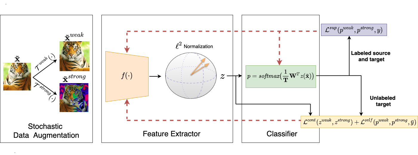
Figure 1: Overview of the Con²DA framework. Our model takes weak and strong augmented samples and passes them through a feature extractor. The resulting vectors are normalized to the unit hypersphere. In the supervised case, the standard cross-entropy is applied for weak and strong augmented data. When labels are not available, a contrastive and a self-supervised loss functions are applied, leveraging both weak and strong augmented samples and extracting consistent feature representations in the normalized representation space. Notice that continuous black lines represent operations performed in the forward pass, while dashed red lines represent operations performed in the backward pass.

In a semi-supervised domain adaptation (SSDA) problem, we are given a source dataset composed by the images and their respective labels $\mathcal{D}^{s}=\{\mathbf{x}_{i}^{s},y_{i}^{s}\}_{i=1}^{n^{s}}$, an unlabeled target dataset $\mathcal{D}^{u}=\{(\mathbf{x}_{i}^{u})\}^{n^{u}}_{i=1}$, and labeled target data $\mathcal{D}^{t}=\{(\mathbf{x}_{i}^{t},y_{i}^{t})\}_{i=1}^{n^{t}}$. In SSDA, $n^{t}$ is assumed to be small (usually 1 or 3 labeled samples per class). For both domains we have the same $K$ classes, i.e. $y^{s}_{i}\in\{1,...,K\}$, $y^{t}_{i}\in\{1,...,K\}$. Our goal is to reduce the domain shift between $\mathcal{D}^{s}$ and $\{\mathcal{D}^{u}$, $\mathcal{D}^{t}\}$, to improve the performance of the model when evaluating on $\mathcal{D}^{u}$.

In this work we propose a method that learns Consistent and Contrastive feature representations for SSDA. An overview of our method, named Con²DA can be seen in Figure 1. Our framework is composed of three major components:

• Stochastic data augmentation: Given an input $\mathbf{x}\in\{\mathcal{D}^{s},\mathcal{D}^{u},\mathcal{D}^{t}\}$, two random transformations are applied, generating the two associated versions of the same sample $\tilde{\mathbf{x}}^{weak}\sim\mathcal{T}^{weak}(\mathbf{x})$ and $\tilde{\mathbf{x}}^{strong}\sim\mathcal{T}^{strong}(\mathbf{x})$. For $\mathcal{T}^{weak}(\cdot)$, we used simple transformations such as random cropping, random horizontal flipping, and Gaussian blur. For $\mathcal{T}^{strong}(\cdot)$, we used the same augmentations, plus RandAugment [6]. We show that by adopting an augmentation strategy that strongly perturbs input images, our algorithm improves in performance compared with the method using only weak augmentations (see Appendix D).

• Feature extractor: We used a feature extractor $f(\cdot)$ that maps transformations $\tilde{\mathbf{x}}\in\{\tilde{\mathbf{x}}^{weak},\tilde{\mathbf{x}}^{strong}\}$ into a representation vector $h=f(\tilde{\mathbf{x}})\in\mathbb{R}^{d}$, where $d$ is the representation dimension (we set $d=256$ in all our experiments). This vector is normalized to the unit hypersphere using the $\ell_{2}$ normalization, that takes the form $z(\cdot)=\frac{f(\cdot)}{\lVert f(\cdot)\rVert}$. Depending on whether $\tilde{\mathbf{x}}$ is a labeled or unlabeled sample, different loss functions are optimized.

• Classifier: We pass the normalized feature representations through a linear classifier $\textbf{W}\in\mathbb{R}^{d\times K}$ and we scale the output by a temperature hyperparameter $T$. Using a softmax activation function we obtained the output probability distribution $p(y|\tilde{\mathbf{x}})=\textit{Softmax}\big{(}\frac{1}{\mathbf{T}}\mathbf{W}^{T}z(\tilde{\mathbf{x}})\big{)}$. It is worth noticing that for accurate classification, both the weight vector and the normalized features of the same class should be pointing to the same direction into the hypersphere. This way, each weight vector $\textbf{w}_{i}\in\textbf{W}$, $i\in\{1,...,K\}$ can be seen as a representative prototype of each class [28].

Supervised Loss Function: For the labeled objects, we align associated data pairs towards their respective class prototype, regardless of whether the objects come from the source or target domain. Specifically, we sample a mini-batch of data $\{(\textbf{x}_{i},y_{i})\}^{N}_{i=1}\in\{\mathcal{D}^{s},\mathcal{D}^{t}\}$, composed of $N/2$ number of source labeled objects and $N/2$ number of target labeled objects. For each sample $\mathbf{x}_{i}$, two stochastic augmentations are applied, obtaining a weak augmented version $\tilde{\mathbf{x}_{i}}^{weak}$, and a strong augmented version $\tilde{\mathbf{x}_{i}}^{strong}$. Both images are passed through the feature extractor and classifier, obtaining the probability vectors $p^{weak}_{i}=p(y_{i}|\tilde{\mathbf{x}}^{weak}_{i})$ and $p^{strong}_{i}=p(y_{i}|\tilde{\mathbf{x}}^{strong}_{i})$. Then, the loss function for each mini-batch can be computed using Equation 1:

$$\mathcal{L}^{sup}=\frac{1}{N}\sum^{N}_{i=1}\big{(}\mathcal{L}_{ce}(p^{weak}_{i},y_{i})+\mathcal{L}_{ce}(p^{strong}_{i},y_{i})\big{)},$$ (1)

where $\mathcal{L}_{ce}$ is a standard cross-entropy loss. Intuitively, by minimizing this objective with respect to the feature extractor and the linear classifier, we force the labeled feature representations and prototypes that represent the same class to point in the same direction into the hypersphere.

Unsupervised Loss Functions: In the unsupervised case, we expect the distance of normalized feature representations of associated data pairs to be low, while we expect the distance with feature representations of objects that were generated from different inputs to be high. For this purpose, we sample a mini-batch $\{\textbf{x}_{i}\}^{N}_{i=1}\in\mathcal{D}^{u}$ of $N$ unlabeled target objects and we use the normalized temperature-scaled cross-entropy loss function (NT-Xent; [3]), that takes two associated normalized feature representations $z^{weak}_{i}=z(\tilde{\textbf{x}}^{weak}_{i})$ and $z^{strong}_{i}=z(\tilde{\textbf{x}}^{strong}_{i})$, and computes the cosine similarity between them $sim(z^{weak}_{i},z^{strong}_{i})=z^{weak}_{i}\cdot z^{strong}_{i}$. This similarity is forced to be high, while the similarities $sim(z_{i},z_{a})$ between each feature representation $z_{i}\in\{z_{i}^{weak},z_{i}^{strong}\}$ and the rest of the dissimilar augmented samples $z_{a}\in A(i)=\{z^{weak}_{1},...,z^{weak}_{i-1},z^{weak}_{i+1},...,z^{weak}_{N}\}\cup\{z^{strong}_{1},...,z^{strong}_{i-1},z^{strong}_{i+1},...,z^{strong}_{N}\}$ are forced to be low. The mathematical formulation for the NT-Xent loss can be written as follows:

$$\mathcal{L}^{cont}=\frac{1}{N}\sum^{N}_{i=1}-log{\frac{\exp(sim(z^{weak}_{i},z^{strong}_{i})/T)}{\sum_{z_{a}\in A(i)}\exp(sim(z_{i},z_{a})/T)}},$$ (2)

where $T$ denotes a temperature hyperparameter. Notice that this loss function is computed for both $z_{i}=z_{i}^{weak}$ and $z_{i}=z_{i}^{strong}$.

Our model also computes an artificial label for each pair of strong and weak augmented unlabeled samples (i.e. pseudo-labeling [22, 19, 31]). This label can be obtained by computing the $\operatorname*{arg\,max}$ function over the averaged model predictions for the $k$ classes, for a given pair of associated samples $\bar{y}_{i}=\operatorname*{arg\,max}_{1\leq k\leq K}((p^{weak}_{ik}+p^{strong}_{ik})/2)$. Similarly, an averaged model confidence can be computed as $\bar{p}_{i}=\max_{1\leq k\leq K}((p^{weak}_{ik}+p^{strong}_{ik})/2)$. Then, for each mini-batch our method minimizes a self-supervised loss function with respect to the feature extractor:

$$\mathcal{L}^{self}=\frac{1}{N}\sum^{N}_{i=1}\big{(}\mathbbm{1}_{{\bar{p}_{i}\geq\tau}}\mathcal{L}_{ce}(p^{weak}_{i},\bar{y}_{i})+\mathbbm{1}_{{\bar{p}_{i}\geq\tau}}\mathcal{L}_{ce}(p^{strong}_{i},\bar{y}_{i})\big{)}$$ (3)

where $\mathbbm{1}_{{\bar{p}_{i}\geq\tau}}\in\{0,1\}$ is the indicator function that takes value $1$ iff $\bar{p}_{i}$ is greater than $\tau$, a probability threshold hyperparameter, and $0$ otherwise. For simplicity, we assume that $\bar{p}_{i}$ are valid one-hot probability distributions for the cross-entropy loss.

The overall optimization procedure can be seen in Appendix E.

3 Experiments

sAs in the standard SSDA scenario, we randomly chose one or three labeled training samples per target class for training (one and three-shot respectively). We also randomly selected three target labeled samples as the validation set. We used all the unlabeled data for training, and we reveal their labels to evaluate and report the final model performance.
Datasets. We performed experiments using three benchmark datasets: DomainNet [25] a large-scale domain adaptation dataset that contains six domains and 345 classes in each domain. Following [28], four domains (R: Real, P: Painting, S: Sketch, C: Clipart), 126 classes, and 7 different adaptation scenarios are used for evaluation. Office-Home [33] contains four domains (R: Real, A: Art, C: Clipart, P: Product) and 65 classes. We performed experiments using 12 adaptation scenarios. Office31 [27] contains three domains (W: Webcam, D: DSLR, A: Amazon), and 31 classes. We used two adaptation scenarios for evaluation (D to A, and W to A).
Baselines. We compared our method against state-of-the-art SSDA and UDA approaches, as well as using no domain adaptation at all. The baselines for SSDA consist of the state-of-the-art methods MME [29], APE [15], and BiAT [13]. For UDA we compared with DANN [9], ADR [29], and CDAN [20]. We trained UDA methods treating target labeled samples as if they were source labeled samples. Non adaptation methods consisted of models trained on all labeled samples using cross-entropy, leveraging only labeled data (S+T; [5]), and considering unlabeled samples by minimizing the conditional entropy (ENT; [11]).
Results A summary of our results is shown in Table 1 (see Appendix C for complete result tables). For the DomainNet dataset, our model achieved competitive results compared to the rest of state-of-the-art methods for AlexNet and ResNet34 in both one and three shot cases. As can be seen for Office-Home our method outperforms the averaged results reported by previous state-of-the-art results by $1.3\%$ of accuracy in average. Finally, for Office31 our model outperforms previous state-of-the-art methods by a margin of $1.0\%$ and $1.4\%$ of accuracy in one-shot and three-shot scenarios respectively.

	DomainNet		Office-Home		Office31		DomainNet
Method	1-shot	3-shot	1-shot	3-shot	1-shot	3-shot	1-shot	3-shot
	AlexNet						ResNet34
S+T [5]	40.0	40.3	44.1	50.0	50.2	61.8	56.9	60.0
DANN [9]	40.4	42.4	45.1	50.3	55.8	64.8	58.4	60.7
ADR [29]	39.2	42.7	44.5	49.5	50.6	61.3	57.6	60.4
CDAN [20]	39.1	41.0	41.2	46.2	49.5	60.9	62.5	66.5
ENT [11]	29.1	39.8	38.8	50.9	50.4	65.1	62.6	67.6
MME [29]	44.2	48.2	49.2	55.2	56.5	67.6	66.4	68.9
APE [15]	44.6	48.9	-	55.6	-	68.3	67.6	71.7
BiAT [13]	45.5	49.4	49.6	56.4	56.3	68.4	67.1	69.7
Con2DA (Ours)	45.5	49.5	50.5	55.8	57.3	69.8	68.4	71.4

Table 1: Mean Accuracy over the different adaptation settings for DomainNet, Office-Home and Office31. All experiments were performed using the same adaptations and data splits used by [28, 15].

4 Conclusions

Despite the huge labeling efforts that deep neural network models need to achieve their best performances, SSDA methods can be applied to greatly reduce labeling costs. In this work, we present Con²DA, a simple framework that learns from artificially augmented images using consistent and contrastive visual representation to improve generalization on target domain. We studied the main components of our model and we showed the effect of different combinations of augmentation and training strategies. Using these findings, we compared our methods with different SSDA and UDA methods and we obtained state-of-the-art performances in three commonly used domain adaptation benchmarks DomainNet, Office-Home, and Office31 by margins of $1.3\%$, $1.3\%$, and $1.4\%$ respectively.

5 Acknowledgements

We gratefully acknowledge support from ANID through the FONDECYT Initiation grant Nº11191130 and from the Data Science Unit at University of Concepción. G.C.V. acknowledges support from the ANID –Millennium Science Initiative Program–ICN12_009 awarded to the Millennium Institute of Astrophysics (MAS).

6 Appendix

Appendix A: Implementation Details:

We implemented our model using PyTorch [24]. For fair comparison with previous methods, we used AlexNet [17] or ResNet34 [12] pretrained on Imagenet [26] as the feature extractor. If the number of labeled objects class in the target domain is greater than 256, we set the batch size to 256. If not, we set the batch size to the number of target labeled objects. We sample two mini-batches, where the first mini-batch contains the same number of labeled objects per domain, and the second mini-batch is composed of only unlabeled target samples. We optimized our model using Adam [16] with hyperparameters $\beta_{1}=$ 0.9, $\beta_{2}=0.999$, and a learning rate of 0.00008 for all experiments. We decayed the learning rate with the cosine decay schedule without restarts as in [21]. In all scenarios, the augmentation policy was set to $H=1$ and the distortion magnitude to $M=10$ (details in Appendix A). The rest of the hyperparameters were set to ($T=0.05$, $\tau=0.9$) for DomainNet, ($T=0.3$, $\tau=0.95$) for Office-Home, and ($T=0.5$, $\tau=0.95$) for Office31. We did a forward pass using the two mini-batches (labeled source and target, and unlabeled target), calculated their respective losses, and did a backward pass. We called each of these forward-backward passes an iteration. We trained each model over 5000 iterations, setting a patience of 50 iterations for early stopping.

Appendix B: Hyperparameter Optimization

We randomly sample three target labeled objects per class as the validation set and we use this set to set the hyperparameters temperature $T$ and threshold $\tau$. We selected the hyperparameters using different domains and adaptation scenarios. Specifically, for Office31 we used the W$\rightarrow$A scenario, and for Office-Home and DomainNet we used the R$\rightarrow$C scenario. We vary the hyperparameters from $T\in\{0.01,0.05,0.07,0.1,0.3,0.5,0.7,0.9\}$ and $\tau\in\{0.8,0.9,0.95\}$.

Figure 2 shows the results in terms of accuracy each case. As can be seen, the best results on validation set are achieved using the hyperparameters ($T=0.05$, $\tau=0.9$) for DomainNet (AlexNet), ($T=0.05$, $\tau=0.8$) for DomainNet (ResNet34), ($T=0.3$, $\tau=0.95$) for Office-Home, and ($T=0.5$, $\tau=0.95$) for Office31. Therefore, we setted the hyperparameters to these values for the remaining adaptation scenarios in each case for the results.

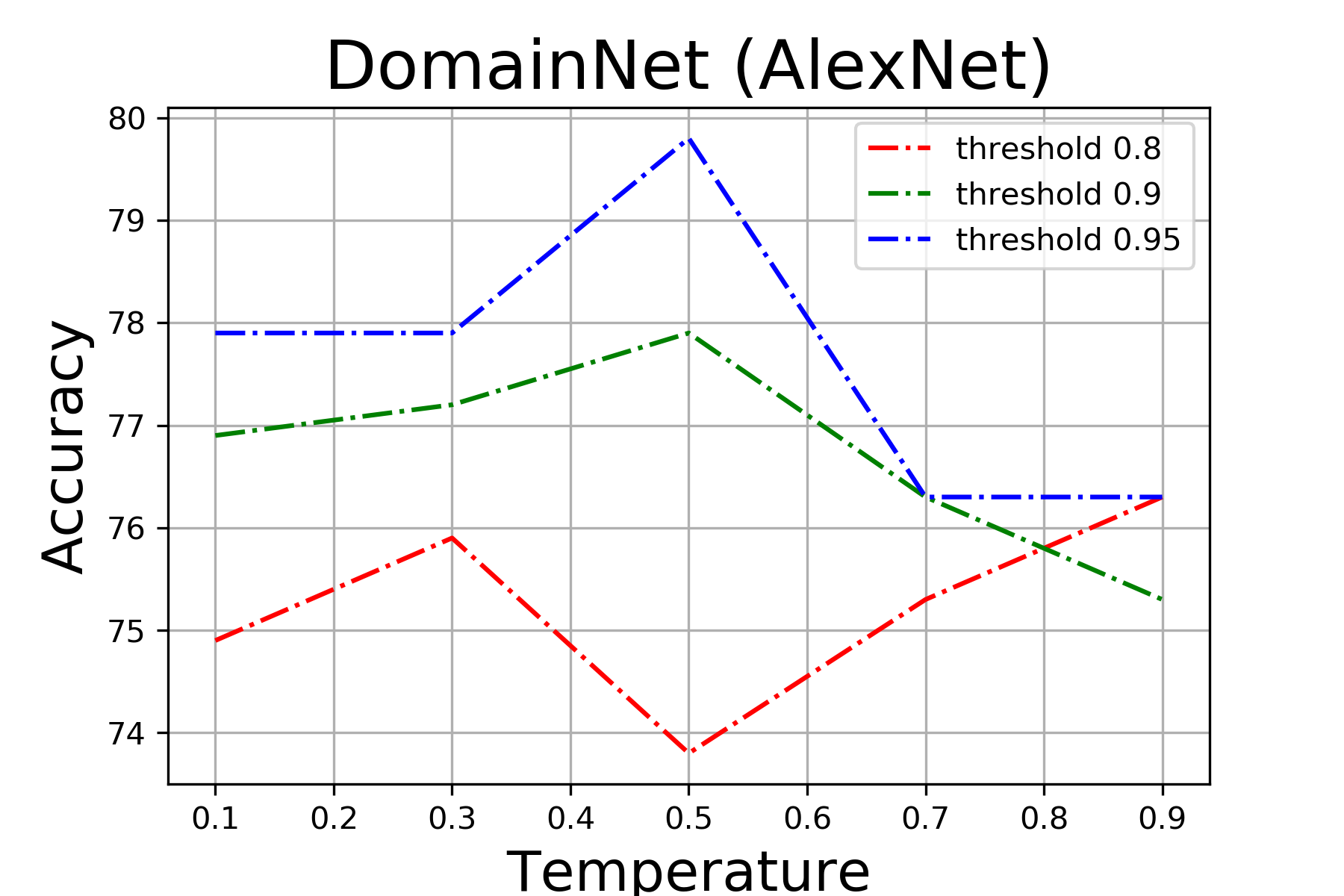
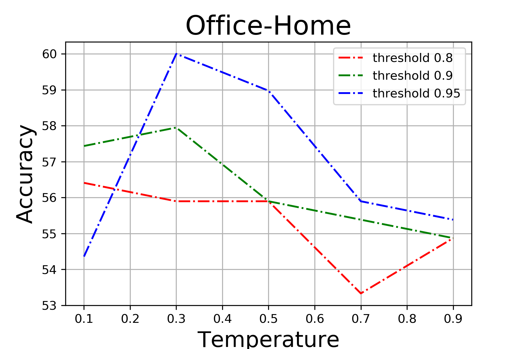
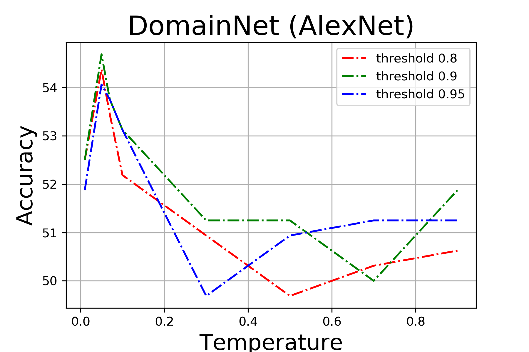
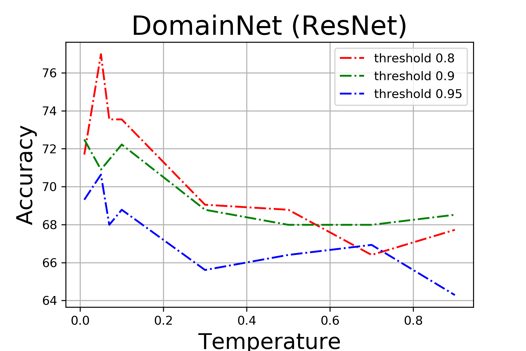
Figure 2: Accuracy for different values of the hyperparatemers threshold and temperature. Results computed for Office31, Office-Home and DomainNet (using AlexNet and ResNet34 model architectures).

Appendix C: Results per adaptaton setting

Results of our method on the DomainNet dataset are shown in Table 2. In both the one and three-shot cases, our model achieved competitive results compared to the rest of state-of-the-art methods for AlexNet and ResNet34. As can be seen in Table 3, for Office-Home our method outperforms the averaged results reported by previous state-of-the-art results by margins between $0.1\%$ up to $1.3\%$ of accuracy. Finally, as can be seen in Table 4, for Office31 our model outperforms previous state-of-the-art methods by a margin of $1.0\%$ and $1.4\%$ of accuracy in one-shot and three-shot scenario respectively.

	R$\rightarrow$ C		R$\rightarrow$ P		P$\rightarrow$ C		C$\rightarrow$ S		S$\rightarrow$ P		R$\rightarrow$ S		P$\rightarrow$ R		Mean
Method	1-shot	3-shot	1-shot	3-shot	1-shot	3-shot	1-shot	3-shot	1-shot	3-shot	1-shot	3-shot	1-shot	3-shot	1-shot	3-shot
	AlexNet
S+T [5]	43.3	47.1	42.4	45.0	40.1	44.9	33.6	36.4	35.7	38.4	29.1	33.3	55.8	58.7	40.0	43.4
DANN [9]	43.3	46.1	41.6	43.8	39.1	41.0	35.9	36.5	36.9	38.9	32.5	33.4	53.6	57.3	40.4	42.4
ADR [29]	43.1	46.2	41.4	44.4	39.3	43.6	32.8	36.4	33.1	38.9	29.1	32.4	55.9	57.3	39.2	42.7
CDAN [20]	46.3	46.8	45.7	45.0	38.3	42.3	27.5	30.2	33.7	33.7	28.8	31.3	56.7	58.7	49.1	41.0
ENT [11]	37.0	45.5	35.6	42.6	26.8	40.4	18.9	31.1	15.1	29.6	18.0	29.6	52.2	60.0	29.1	39.8
MME [29]	48.9	55.6	48.0	49.0	46.7	51.7	36.3	39.4	39.4	43.0	33.3	37.9	56.8	60.7	44.2	48.2
APE [15]	47.7	54.6	49.0	50.0	46.9	52.1	38.5	42.6	38.5	42.2	33.8	38.7	57.5	61.4	44.6	48.9
BiAT [13]	54.2	58.6	49.2	50.6	44.0	52.0	37.7	41.9	39.6	42.1	37.2	42.0	56.9	58.8	45.5	49.4
Con2DA (Ours)	50.0	54.5	50.3	51.6	47.7	53.5	36.9	42.6	35.4	40.3	35.9	39.2	62.7	64.8	45.5	49.5
	ResNet34
S+T [5]	55.6	60.0	60.6	62.2	56.8	59.4	50.8	55.0	56.0	59.5	46.3	50.1	71.8	73.9	56.9	60.0
DANN [9]	58.2	59.8	61.4	62.8	56.3	59.6	52.8	55.4	57.4	59.9	52.2	54.9	70.3	72.2	58.4	60.7
ADR [29]	57.1	60.7	61.3	61.9	57.0	60.7	51.0	54.4	56.0	59.9	49.0	51.1	72.0	74.2	57.6	60.4
CDAN [20]	65.0	69.0	64.9	67.3	63.7	68.4	53.1	57.8	63.4	65.3	54.5	59.0	73.2	78.5	62.5	66.5
ENT [11]	65.2	71.0	65.9	69.2	65.4	71.1	54.6	60.0	59.7	62.1	52.1	61.1	75.0	78.6	62.6	67.6
MME [29]	70.0	72.2	67.7	69.7	69.0	71.7	56.3	61.8	64.8	66.8	61.0	61.9	76.1	78.5	66.4	68.9
APE [15]	70.4	76.6	70.8	72.1	72.9	76.7	56.7	63.1	64.5	66.1	63.0	67.8	76.6	79.4	67.6	71.7
BiAT [13]	73.0	74.9	68.0	68.8	71.6	74.6	57.9	61.5	63.9	67.5	58.5	62.1	77.0	78.6	67.1	69.7
Con2DA (Ours)	71.3	74.2	71.8	72.1	71.1	75.0	60.0	65.7	63.5	67.1	65.2	67.1	75.7	78.6	68.4	71.4

Table 2: Accuracy on DomainNet ($\%$) using AlexNet [17] and ResNet34 [12].

Method	R$\rightarrow$ C	R$\rightarrow$ P	R$\rightarrow$ A	P$\rightarrow$ R	P$\rightarrow$ C	P$\rightarrow$ A	A$\rightarrow$ P	A$\rightarrow$ C	A$\rightarrow$ R	C$\rightarrow$ R	C$\rightarrow$ A	C$\rightarrow$ P	Mean
	One-shot
S+T [5]	37.5	63.1	44.8	54.3	31.7	31.5	48.8	31.1	53.3	48.5	33.9	50.8	44.1
DANN [9]	42.5	64.2	45.1	56.4	36.6	32.7	43.5	34.4	51.9	51.0	33.8	49.4	45.1
ADR [29]	37.8	63.5	45.4	53.5	32.5	32.2	49.5	31.8	53.4	49.7	34.2	50.4	44.5
CDAN [20]	36.1	62.3	42.2	52.7	28.0	27.8	48.7	28.0	51.3	41.0	26.8	49.9	41.2
ENT [11]	26.8	65.8	45.8	56.3	23.5	21.9	47.4	22.1	53.4	30.8	18.1	53.6	38.8
MME [29]	42.0	69.6	48.3	58.7	37.8	34.9	52.5	36.4	57.0	54.1	39.5	59.1	49.2
BiAT [13]	-	-	-	-	-	-	-	-	-	-	-	-	49.6
Con2DA (Ours)	43.7	70.7	47.8	60.4	39.8	36.8	62.5	36.9	58.5	53.0	35.4	60.0	50.5
	Three-shot
S+T [5]	44.6	66.7	47.7	57.8	44.4	36.1	57.6	38.8	57.0	54.3	37.5	57.9	50.0
DANN [9]	47.2	66.7	46.6	58.1	44.4	36.1	57.2	39.8	56.6	54.3	38.6	57.9	50.3
ADR [29]	45.0	66.2	46.9	57.3	38.9	36.3	57.5	40.0	57.8	53.4	37.3	57.7	49.5
CDAN [20]	41.8	69.9	43.2	53.6	35.8	32.0	56.3	34.5	53.5	49.3	27.9	56.2	46.2
ENT [11]	44.9	70.4	47.1	60.3	41.2	34.6	60.7	37.8	60.5	58.0	31.8	63.4	50.9
MME [28]	51.2	73.0	50.3	61.6	47.2	40.7	63.9	43.8	61.4	59.9	44.7	64.7	55.2
APE [15]	51.9	74.6	51.2	61.6	47.9	42.1	65.5	44.5	60.9	58.1	44.3	64.8	55.6
BiAT [13]	-	-	-	-	-	-	-	-	-	-	-	-	56.4
Con2DA (Ours)	52.3	73.5	49.1	64.4	49.3	38.2	66.4	47.7	62.4	59.9	39.9	66.1	55.8

Table 3: Accuracy on Office-Home ($\%$) 3-shot using AlexNet [17].

	W$\rightarrow$ A		D$\rightarrow$ A		Mean
Method	1-shot	3-shot	1-shot	3-shot	1-shot	3-shot
S+T [5]	50.4	61.2	50.0	62.4	50.2	61.8
DANN [9]	57.0	64.4	54.5	65.2	55.8	64.8
ADR [29]	50.2	61.2	50.9	61.4	50.6	61.3
CDAN [20]	50.4	60.3	48.5	61.4	49.5	60.9
ENT [11]	50.7	64.0	50.0	66.2	50.4	65.1
MME [29]	57.2	67.3	55.8	67.8	56.5	67.6
APE [15]	-	67.6	-	69.0	-	68.3
BiAT [13]	57.9	68.2	54.6	68.5	56.3	68.4
Con2DA (Ours)	58.3	69.8	56.2	69.7	57.3	69.8

Table 4: Accuracy on Office-31 ($\%$) using AlexNet.

Appendix D: Ablation Study

In order to understand the key components of our method, we performed an ablation study to compare gains in performance using variations of our algorithm. We first investigated the performance of different strong augmentation policies. We started by first measuring the performance on a baseline where no strong augmentations are applied (i.e both $\tilde{\mathbf{x}}^{weak}$ and $\tilde{\mathbf{x}}^{strong}$ are samples from $\mathcal{T}^{weak}$). In a three-shot scenario, the accuracy on validation set is $72.0\%$ for Office31 in the W$\rightarrow$A setting, and $50.5\%$ for DomainNet in the R$\rightarrow$ C setting. We added strong augmentation policies to $\tilde{\mathbf{x}}^{strong}$ such as color jitter, random grayscale, Cutout [7], and RandAugment [6]. The performance between combinations of these augmentation policies is shown in Figure 3. As can be seen, our model consistently improved the baseline and the rest of the augmentation strategies in both settings by using RandAugment as a strong augmentation policy. Using RandAugment, we also investigate the model performance removing components from the loss function. Firstly, we removed the contrastive loss function defined in Equation 2 (w/o $\mathcal{L}_{cont}$), the self-supervised loss function defined in Equation 3, w/o $\mathcal{L}_{self}$. Then, we forced the prototypes to be unit vectors by normalizing the linear classifier W, and we computed the cosine similarity between the normalized linear classifier and feature vector (w cosine). Results of these variations are shown in Table 5. As can be seen, our algorithm is benefited from the use of contrastive and self-supervised loss. Finally, the linear classifier without normalization helped our model to obtain significant performance improvements.

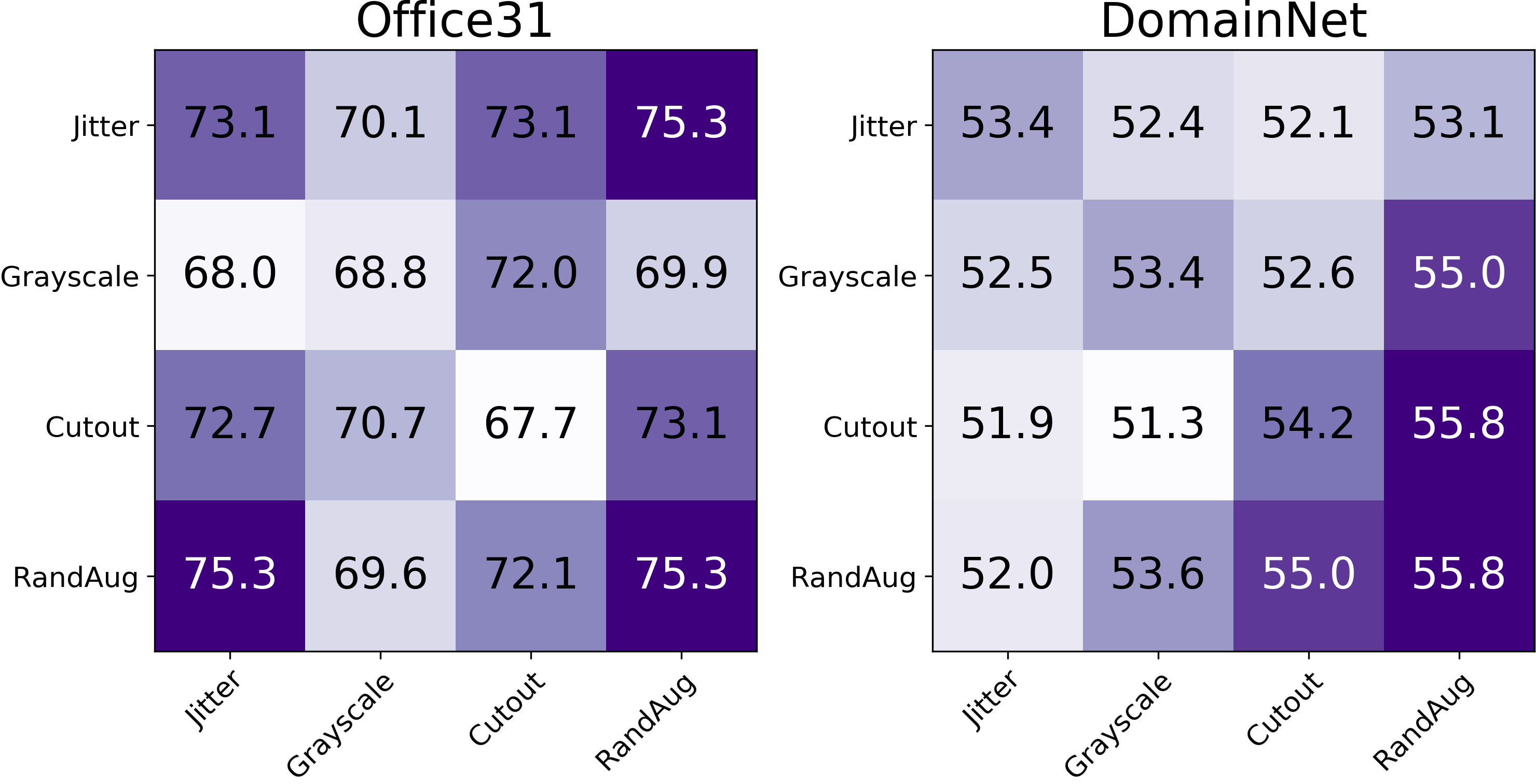
Figure 3: Comparison of different augmentation policies for Office31 (W$\rightarrow$ A) and DomainNet (R$\rightarrow$ C) in a three-shot scenario. Performance measured on the validation set.

	W$\rightarrow$ A	R$\rightarrow$ C
w/o $\mathcal{L}_{cont}$	66.7	54.5
w/o $\mathcal{L}_{self}$	73.1	51.8
w cosine	72.0	55.7
Con2DA	75.3	55.8

Table 5: Accuracy ($\%$) of different training strategies for Office31 (W$\rightarrow$ A) and DomainNet (R$\rightarrow$ C) in a three-shot scenario. Performance measured on the validation set.

Appendix E: Algorithm Algorithm 1 summarizes the Con²DA training procedure.

Algorithm 1 Con²DA Training procedure.

1:Mini-batches $\{\textbf{x}_{i},y_{i}\}^{N}_{i=1}\in\{\mathcal{D}^{s},\mathcal{D}^{t}\}$ and $\{\textbf{x}^{u}_{i}\}^{N}_{i=1}\in\mathcal{D}^{u}$. Hyperparameters $\tau$ and $T$. Transformations $\mathcal{T}^{weak}$ and $\mathcal{T}^{strong}$. Feature extractor $f$ and linear classifier $\mathbf{W}$.

2:while not converged do:

3:   for $i\in\{1,...,N\}$ do

4:      # Augmentations for labeled data

5:      $\tilde{\textbf{x}}^{weak}_{i}\sim\mathcal{T}^{weak}(\textbf{x}_{i})$

6:      $\tilde{\textbf{x}}^{strong}_{i}\sim\mathcal{T}^{strong}(\textbf{x}_{i})$

7:      # Probability vectors for labeled samples.

8:      $p^{weak}_{i}=p(y_{i}|\tilde{\textbf{x}}^{weak}_{i})$

9:      $p^{strong}_{i}=p(y_{i}|\tilde{\textbf{x}}^{strong}_{i})$

10:      # Augmentations for unlabeled data

11:      $\tilde{\textbf{x}}^{u,weak}_{i}\sim\mathcal{T}^{weak}(\textbf{x}_{i}^{u})$

12:      $\tilde{\textbf{x}}^{u,strong}_{i}\sim\mathcal{T}^{strong}(\textbf{x}_{i}^{u})$

13:      # Normalized feature representations.

14:      $z^{u,weak}_{i}=f(\tilde{\textbf{x}}^{u,weak}_{i}))/\lVert f(\tilde{\textbf{x}}^{u,weak}_{i}))\rVert$

15:      $z^{u,strong}_{i}=f(\tilde{\textbf{x}}^{u,strong}_{i}))/\lVert f(\tilde{\textbf{x}}^{u,strong}_{i}))\rVert$

16:      # Probability vectors for unlabeled samples.

17:      $p^{u,weak}_{i}=p(y_{i}|\tilde{\textbf{x}}^{u,weak}_{i})$

18:      $p^{u,strong}_{i}=p(y_{i}|\tilde{\textbf{x}}^{u,strong}_{i})$

19:      # Averaged prediction and pseudo-label.

20:      $\bar{p}_{i}=\max_{1\leq k\leq K}((p^{u,weak}_{ik}+p^{u,strong}_{ik})/2)$

21:      $\bar{y}_{i}=\operatorname*{arg\,max}_{1\leq k\leq K}((p^{u,weak}_{ik}+p^{u,strong}_{ik})/2)$

22:   end for

23:   for $i\in\{1,...,N\}$ do

24:      $sim_{ii}=z^{u,weak}_{i}\cdot z^{u,strong}_{i}$

25:      Define $A(i)$

26:      for $z_{a}\in A(i)$ do

27:         $sim_{ia}=z^{u}_{i}\cdot z^{a}$

28:      end for

29:   end for

30:   Compute Equations 1, 2, and 3

31:   Update parameters of $f$ and $W$ to minimize Eq. 1.

32:   Update parameters of $f$ to minimize Eq. 2 and 3.

33:end while

34:Trained feature extractor $f$ and classifier $\mathbf{W}$

References

- [1] Shai Ben-David, John Blitzer, Koby Crammer, and Fernando Pereira. Analysis of representations for domain adaptation. In B. Schölkopf, J. Platt, and T. Hoffman, editors, Advances in Neural Information Processing Systems, volume 19, pages 137–144. MIT Press, 2007.
- [2] David Berthelot, Nicholas Carlini, Ekin D. Cubuk, Alex Kurakin, Kihyuk Sohn, Han Zhang, and Colin Raffel. Remixmatch: Semi-supervised learning with distribution matching and augmentation anchoring. In 8th International Conference on Learning Representations, ICLR 2020, Addis Ababa, Ethiopia, April 26-30, 2020. OpenReview.net, 2020.
- [3] Ting Chen, Simon Kornblith, Mohammad Norouzi, and Geoffrey Hinton. A simple framework for contrastive learning of visual representations. In Hal Daumé III and Aarti Singh, editors, Proceedings of the 37th International Conference on Machine Learning, volume 119 of Proceedings of Machine Learning Research, pages 1597–1607. PMLR, 13–18 Jul 2020.
- [4] Wei-Yu Chen, Yen-Cheng Liu, Zsolt Kira, Yu-Chiang Wang, and Jia-Bin Huang. A closer look at few-shot classification. In International Conference on Learning Representations, 2019.
- [5] Wei-Yu Chen, Yen-Cheng Liu, Zsolt Kira, Yu-Chiang Frank Wang, and Jia-Bin Huang. A closer look at few-shot classification. CoRR, abs/1904.04232, 2019.
- [6] E. D. Cubuk, B. Zoph, J. Shlens, and Q. V. Le. Randaugment: Practical automated data augmentation with a reduced search space. In 2020 IEEE/CVF Conference on Computer Vision and Pattern Recognition Workshops (CVPRW), pages 3008–3017, 2020.
- [7] Terrance Devries and Graham W. Taylor. Improved regularization of convolutional neural networks with cutout. CoRR, abs/1708.04552, 2017.
- [8] Alexey Dosovitskiy, Jost Tobias Springenberg, Martin Riedmiller, and Thomas Brox. Discriminative unsupervised feature learning with convolutional neural networks. In Proceedings of the 27th International Conference on Neural Information Processing Systems - Volume 1, NIPS’14, page 766–774, Cambridge, MA, USA, 2014. MIT Press.
- [9] Yaroslav Ganin and Victor Lempitsky. Unsupervised domain adaptation by backpropagation. In Francis Bach and David Blei, editors, Proceedings of the 32nd International Conference on Machine Learning, volume 37 of Proceedings of Machine Learning Research, pages 1180–1189, Lille, France, 07–09 Jul 2015. PMLR.
- [10] S. Gidaris and N. Komodakis. Dynamic few-shot visual learning without forgetting. In 2018 IEEE/CVF Conference on Computer Vision and Pattern Recognition, pages 4367–4375, 2018.
- [11] Yves Grandvalet and Yoshua Bengio. Semi-supervised learning by entropy minimization. In Proceedings of the 17th International Conference on Neural Information Processing Systems, NIPS’04, page 529–536, Cambridge, MA, USA, 2004. MIT Press.
- [12] K. He, X. Zhang, S. Ren, and J. Sun. Deep residual learning for image recognition. In 2016 IEEE Conference on Computer Vision and Pattern Recognition (CVPR), pages 770–778, 2016.
- [13] Pin Jiang, Aming Wu, Yahong Han, Yunfeng Shao, Meiyu Qi, and Bingshuai Li. Bidirectional adversarial training for semi-supervised domain adaptation. In Christian Bessiere, editor, Proceedings of the Twenty-Ninth International Joint Conference on Artificial Intelligence, IJCAI-20, pages 934–940. International Joint Conferences on Artificial Intelligence Organization, 7 2020. Main track.
- [14] Prannay Khosla, Piotr Teterwak, Chen Wang, Aaron Sarna, Yonglong Tian, Phillip Isola, Aaron Maschinot, Ce Liu, and Dilip Krishnan. Supervised contrastive learning. arXiv preprint arXiv:2004.11362, 2020.
- [15] Taekyung Kim and Changick Kim. Attract, perturb, and explore: Learning a feature alignment network for semi-supervised domain adaptation. In Andrea Vedaldi, Horst Bischof, Thomas Brox, and Jan-Michael Frahm, editors, Computer Vision – ECCV 2020, pages 591–607, Cham, 2020. Springer International Publishing.
- [16] Diederik P. Kingma and Jimmy Ba. Adam: A method for stochastic optimization. CoRR, abs/1412.6980, 2015.
- [17] Alex Krizhevsky, Ilya Sutskever, and Geoffrey E Hinton. Imagenet classification with deep convolutional neural networks. In F. Pereira, C. J. C. Burges, L. Bottou, and K. Q. Weinberger, editors, Advances in Neural Information Processing Systems 25, pages 1097–1105. Curran Associates, Inc., 2012.
- [18] Samuli Laine and Timo Aila. Temporal ensembling for semi-supervised learning. In 5th International Conference on Learning Representations, ICLR 2017, Toulon, France, April 24-26, 2017, Conference Track Proceedings. OpenReview.net, 2017.
- [19] Dong-Hyun Lee. Pseudo-label : The simple and efficient semi-supervised learning method for deep neural networks. ICML 2013 Workshop : Challenges in Representation Learning (WREPL), 07 2013.
- [20] Mingsheng Long, ZHANGJIE CAO, Jianmin Wang, and Michael I Jordan. Conditional adversarial domain adaptation. In S. Bengio, H. Wallach, H. Larochelle, K. Grauman, N. Cesa-Bianchi, and R. Garnett, editors, Advances in Neural Information Processing Systems 31, pages 1640–1650. Curran Associates, Inc., 2018.
- [21] Ilya Loshchilov and Frank Hutter. SGDR: stochastic gradient descent with warm restarts. In 5th International Conference on Learning Representations, ICLR 2017, Toulon, France, April 24-26, 2017, Conference Track Proceedings. OpenReview.net, 2017.
- [22] G. J. McLachlan. Iterative reclassification procedure for constructing an asymptotically optimal rule of allocation in discriminant analysis. Journal of the American Statistical Association, 70(350):365–369, 1975.
- [23] S. J. Pan and Q. Yang. A survey on transfer learning. IEEE Transactions on Knowledge and Data Engineering, 22(10):1345–1359, Oct 2010.
- [24] Adam Paszke, Sam Gross, Francisco Massa, Adam Lerer, James Bradbury, Gregory Chanan, Trevor Killeen, Zeming Lin, Natalia Gimelshein, Luca Antiga, Alban Desmaison, Andreas Kopf, Edward Yang, Zachary DeVito, Martin Raison, Alykhan Tejani, Sasank Chilamkurthy, Benoit Steiner, Lu Fang, Junjie Bai, and Soumith Chintala. Pytorch: An imperative style, high-performance deep learning library. In H. Wallach, H. Larochelle, A. Beygelzimer, F. d'Alché-Buc, E. Fox, and R. Garnett, editors, Advances in Neural Information Processing Systems 32, pages 8024–8035. Curran Associates, Inc., 2019.
- [25] Xingchao Peng, Qinxun Bai, Xide Xia, Zijun Huang, Kate Saenko, and Bo Wang. Moment matching for multi-source domain adaptation. In Proceedings of the IEEE International Conference on Computer Vision, pages 1406–1415, 2019.
- [26] Olga Russakovsky, Jia Deng, Hao Su, Jonathan Krause, Sanjeev Satheesh, Sean Ma, Zhiheng Huang, Andrej Karpathy, Aditya Khosla, Michael Bernstein, Alexander C. Berg, and Li Fei-Fei. ImageNet Large Scale Visual Recognition Challenge. International Journal of Computer Vision (IJCV), 115(3):211–252, 2015.
- [27] Kate Saenko, Brian Kulis, Mario Fritz, and Trevor Darrell. Adapting visual category models to new domains. In Proceedings of the 11th European Conference on Computer Vision: Part IV, ECCV’10, page 213–226, Berlin, Heidelberg, 2010. Springer-Verlag.
- [28] Kuniaki Saito, Donghyun Kim, Stan Sclaroff, Trevor Darrell, and Kate Saenko. Semi-supervised domain adaptation via minimax entropy. ICCV, 2019.
- [29] Kuniaki Saito, Kohei Watanabe, Yoshitaka Ushiku, and Tatsuya Harada. Maximum classifier discrepancy for unsupervised domain adaptation. In Proceedings of the IEEE Conference on Computer Vision and Pattern Recognition, pages 3723–3732, 2018.
- [30] Karen Simonyan and Andrew Zisserman. Very deep convolutional networks for large-scale image recognition. In Yoshua Bengio and Yann LeCun, editors, 3rd International Conference on Learning Representations, ICLR 2015, San Diego, CA, USA, May 7-9, 2015, Conference Track Proceedings, 2015.
- [31] Kihyuk Sohn, David Berthelot, Chun-Liang Li, Zizhao Zhang, Nicholas Carlini, Ekin D. Cubuk, Alex Kurakin, Han Zhang, and Colin Raffel. Fixmatch: Simplifying semi-supervised learning with consistency and confidence, 2020.
- [32] Baochen Sun and Kate Saenko. Deep coral: Correlation alignment for deep domain adaptation. In ECCV 2016 Workshops, 2016.
- [33] H. Venkateswara, J. Eusebio, S. Chakraborty, and S. Panchanathan. Deep hashing network for unsupervised domain adaptation. In 2017 IEEE Conference on Computer Vision and Pattern Recognition (CVPR), pages 5385–5394, 2017.
- [34] Z. Wu, Y. Xiong, S. X. Yu, and D. Lin. Unsupervised feature learning via non-parametric instance discrimination. In 2018 IEEE/CVF Conference on Computer Vision and Pattern Recognition, pages 3733–3742, 2018.
- [35] Qizhe Xie, Zihang Dai, Eduard Hovy, Minh-Thang Luong, and Quoc V Le. Unsupervised data augmentation for consistency training. arXiv preprint arXiv:1904.12848, 2019.