Physical Properties of the Supernova Remnant Population in the Small Magellanic Cloud

Abstract

The X-ray emission from a supernova remnant is a powerful diagnostic of the state of its shocked plasma. The temperature and the emission measure are related to the energy of the explosion, the age of the remnant, and the density of the surrounding medium. Here we present the results of a study of the remnant population of the Small Magellanic Cloud. Progress in X-ray observations of remnants has resulted in a sample of 20 remnants in the Small Magellanic Clound with measured temperatures and emission measures. We apply spherically symmetric supernova remnant evolution models to this set of remnants, to estimate ages, explosion energies, and circumstellar medium densities. The distribution of ages yields a remnant birthrate of $\sim$1/1200 yr. The energies and densities are well fit with log-normal distributions, with means of 1.6$\times 10^{51}$ erg and 0.14 cm^-3, and 1$\sigma$ dispersions of a factor of 1.87 in energy and 3.06 in density, respectively.

1 Introduction

The study of supernova remnants (SNRs) is important for astrophysics, including the understanding of injection of energy (e.g. Cox 2005) and elements into the interstellar medium (e.g. Vink 2012). Valuable constraints for stellar evolution and the evolution of the interstellar medium and the Galaxy can be obtained from SNR studies. The goals of SNR research include understanding explosions of supernovae (SN) and the resulting energy and mass injection into the interstellar medium.

Approximately 300 SNRs have been observed in our Galaxy (e.g. Vink 2012). Several historical SNRs have been modelled with hydrodynamic simulations (e.g. Badenes et al. 2006). For many other SNRs, it has been customary to apply a simple Sedov model with an assumed energy and ISM density. Better modelling is required to derive reliable energies, densities and ages from observations. A set of SNR models for spherically symmetric SNRs, which are based on hydrodynamic calculations have been developed by Leahy et al. (2019). These models calculate emission measures (EM) and EM-weighted temperatures for forward-shocked and for reverse-shocked gas. The resulting SNR models allow the use of X-ray observations to estimate SNR physical properties. 43 Galactic SNRs with X-ray spectra and distances were modeled in this way by Leahy et al. (2020) with resulting distributions of ISM density, explosion energy and SNR ages derived for this set. This work showed, not surprisingly, that the range of energies and densities was large. The distributions densities and explosion energies were found to be well-described by log-normal functions. The age distribution was fit to obtain the SNR birthrate.

Our nearby galaxies, the Large and Small Magellanic Clouds (LMC and SMC) are at well known distances of 50 kpc and 60 kpc, respectively ( Pietrzyński et al. 2019 ; Hilditch et al. 2005; Graczyk et al. 2014). They are close enough that we can detect and spatially resolve SNRs from radio to X-ray wavelengths, and are located behind only a moderate Galactic foreground (N_H of a few $10^{20}$ cm^-2; Dickey & Lockman 1990). Models for the SNR population of the LMC and their ages, densities and energies, were presented by Leahy (2017).

Here we study the SNR population of the SMC. This work includes the following. The sample of 19 SMC SNRs with measured X-ray EM and kT from Maggi et al. (2019) is used, supplemented by SNR E0102-7219. SNR E0102-7219 is the brightest SNR in the SMC, and has been extensively studied in X-rays (e.g. Long et al. 2020, Alan et al. 2019, Sasaki et al. 2001 Rasmussen et al. 2001). We apply the models of Leahy et al. (2019), using the solution to the inverse problem as described in Leahy et al. (2020) to obtain SNR best fit properties and their uncertainties. The structure of the paper is as follows. In Section 2 we describe the sample of SMC SNRs then provide an overview of the SNR models and the application to the SMC SNR sample. The results of model fits are given in Section 3. In Section 4 we discuss the results, including comparison of statistical properties of the SMC SNR population with the LMC and Galactic SNR populations. The conclusions are summarized in Section 5.

2 Data and Model Description

2.1 The SNR Sample

For modelling we assume a common distance of 60 kpc to all SNRs and take SMC ISM abundances from column 1 of Table 3 in Maggi et al. (2019). The basic parameters of the 19 SNRs were obtained from Table A.3 of Maggi et al. (2019). The SMC SNR E0102-7219 (MCSNR J0104-7201) is not included in the X-ray spectral analysis of Maggi et al. (2019). It is the only one of the SMC SNRs of Table A.1 of Maggi et al. (2019) that is not included in their spectral analysis, thus we obtain its X-ray spectral parameters from Alan et al. (2019). For each SNR, the EM and EM-weighted temperature were derived from the X-ray studies. The average of semi-major and semi-minor axes from Table A.1 in Maggi et al. (2019) was used as the outer shock radius for input to the spherical SNR model.

For SNRs which are faint in X-rays, which applies to most of the SMC SNRs, the classification as CC type or Ia type depends on whether the X-ray spectrum shows enhanced O, Ne and Mg (CC-type) or enhanced Fe (Type Ia). The Fe enhancements in the X-ray spectra of IKT 5 (SNR) J0047-73.14), IKT 25 (SNR J0104-7205), and DEM S 128 (SNR J0105-7210) are used by Maggi et al. (2019) to classify these SNRs as Type Ia. However Roper et al. (2015) raise questions about the Type Ia classification of these three SNRs, suggesting that they may be CC type SNRs. They point out that although they are overabundant in Fe, they show other features, including potential point sources, X-ray asymmetry, and radio optical and infrared features that are not typical of Type Ia SNRs. Thus we mark these three SNRs as uncertain Type Ia by “Ia?”.

2.2 The Model for SNR Evolution

A SNR is the interaction of the SN ejecta with the circumstellar/interstellar medium (CSM/ISM). The various stages of evolution of a SNR are labelled the ejecta-dominated stage (ED), the adiabatic or Sedov-Taylor stage (ST), the radiative pressure-driven snowplow (PDS) and the radiative momentum-conserving shell (MCS). These stages are reviewed in, e.g., Cioffi et al. (1988), Truelove & McKee (1999) (hereafter TM99), Vink (2012) and Leahy & Williams (2017). In addition, there are the transitions between stages, called ED to ST, ST to PDS, and PDS to MCS, respectively. The ED to ST stage is important because the SNR is still bright, and it is long-lived enough that a significant fraction of SNRs are likely in this phase. For example, a type II SNR with ejecta mass of 10 M_⊙ and average explosion energy of $5\times 10^{50}$ erg (Leahy et al., 2020) in an ISM density of 0.1 cm^-3, is in the ED phase up to age $\sim$4000 yr, and in the ED to ST transition phase until age $\sim$23000 yr (Leahy et al., 2019) .

For simplicity our models assume that the SN ejecta and CSM/ISM are spherically symmetric. The CSM/ISM density profile is a power-law centred on the SN explosion, given by $\rho_{ISM}=\rho_{s}r^{-s}$, with s=0 (constant density medium) or s=2 (stellar wind density profile). The unshocked ejectum has a power-law density $\rho_{ej}\propto r^{-n}$. With these profiles, the ED phase of the SNR evolution has a self-similar evolution (Chevalier 1982 and Nadezhin 1985). The evolution of SNR shock radius was extended for the ED to ST and ST phases by TM99.

A detailed description of the SNR evolution model is given in Leahy et al. (2019) and Leahy & Williams (2017). The forward model, using initial SNR conditions and calculating conditions at time t, is described in Leahy et al. (2019). The input parameters of the SNR forward model are: age; SN energy $E_{0}$; ejected mass $M_{ej}$; ejecta power-law index n; ejecta composition; ISM temperature $T_{ISM}$; ISM composition; ISM power-law index s (0 or 2); and ISM density $n_{0}$ (if s=0) or mass-loss parameter $\rho_{s}=\frac{\dot{M}}{4\pi v_{w}}$ (if s=2). The method of application to observations of SNRs is given by Leahy et al. (2020). Essentially the SNR evolution based on the initial conditions of the explosion is inverted so that the initial quantities are calculated from the SNR current observed properties. The inverse problem is solved by an iterative procedure to obtain a unique solution for density, energy and age for specified values of $s$ and $n$.

2.3 Application of Models to the Sample

We apply two sets of models to the SNR sample. The first set of models is applied to the full sample of 20 SNRs. We fit the data with a single hot plasma component, which is taken to be emission from gas heated by the forward shock (FS) and set $s=0$, $n=7$ . The outer part of the envelope of Type Ia progenitors has a density profile with $n=7$ (Colgate & McKee, 1969). For Type II/CC progenitors, the envelopes may have steeper radial profiles (Chevalier, 1982), with values of $n$ from 7 to 12.5. For the Type Ia? or unknown type SNRs we set the ejecta mass $M_{ej}$=1.4$M_{\odot}$ and for the CC SNRs we set $M_{ej}$=5 $M_{\odot}$. This is called the Standard Model. For E0102-7219, the inferred progenitor mass is 40 $M_{\odot}$ (Alan et al., 2019), thus we run additional models with ejected mass of 20 and 40 $M_{\odot}$: the first corresponds to a 50% mass loss prior to explosion, and the second to no mass loss. The values for those cases are added as a footnote to Table 1, and yield a $\sim$15% and $\sim$30% increase in age; a $\sim$7% and $\sim$10% decrease in energy; and a $\sim$6% and $\sim$12% decrease in density, respectively.

The second set of models is carried out for those 6 SNRs with two measured hot plasma components for the whole SNR: 5 from Maggi et al. (2019) and E0102-7219 from Alan et al. (2019). The two components are from the forward shocked gas and the reverse shocked gas, with the reverse shocked gas identified by its enhanced element abundances. For the second set of models, $R_{FS}$, $EM_{FS}$ and $kT_{FS}$ as taken as model inputs and we compute predicted $EM_{RS}$ and $kT_{RS}$ for different $s$, $n$ cases to test which $s$, $n$ best describe the data.

3 Results of SNR Models

The results from the Standard Model model are shown in Table 1. Derived ages, energies and densities and their uncertainties are given. Uncertainties were found by running models with the input parameters set to their upper and lower limits in different combinations and choosing the largest deviation from the results for the best-fit input parameters.

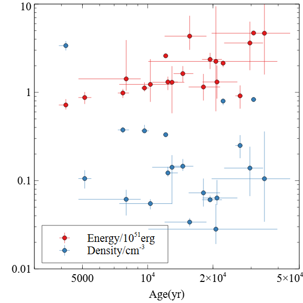
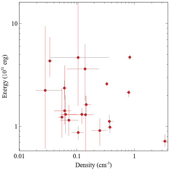
Figure 1: Left panel: Energy and density vs. age for the 20 SNRs from the standard model (forward shock from an SNR with ISM and ejecta profiles with $s=0$, $n=7$). Right panel: Energy vs. density for the 20 SNRs from the standard model.

The left panel of Figure 1 shows the derived explosion energies and ISM densities vs. SNR ages, and the right panel shows the explosion energies vs. ISM densities. The SNR ages range from $\sim$4000 yr to 35000 yr, the explosion energies range from $\sim$0.7 to 5$\times 10^{51}$ erg, and the ISM densities range from $\sim$0.03 to 3 cm^-3. The figures illustrates the wide range of all three parameters and lack of correlation between them for the SNR sample. Analysis of the results of the Standard Model are discussed in Section 4.1 below.

We apply our model to the 6 SNRs with a second X-ray emission component for 6 different cases of (s,n): (0,7), (0,10), (2,6), (2,7), (2,8) and (2,10). The $s$=0 cases are for a uniform circumstellar medium and $s$=2 cases are for a stellar wind density profile. Type Ia could be either, depending on whether or not the white dwarf has a companion with a strong stellar wind. CC SNRs can be either, depending on the presence or not of a strong stellar wind for a long enough time prior to explosion. More $n$ values are chosen for the $s$=2 case because the effect of changing $n$ is stronger for $s$=2 than for $s$=0 (Leahy et al., 2019). The model returns the age, energy and density required in order to reproduce the forward shock. We calculate the properties of the reverse shock ($EM_{RS}$ and $kT_{RS}$) from the model for these different cases and give the results in Table 2. Table 2 also gives the observed values of $EM_{RS}$ and $kT_{RS}$ obtained from fitting the observed X-ray spectrum.

The reverse shock EM increases as $n$ increases, and is larger for $s$=2 than $s$=0 (see Table 2). The reverse shock kT is larger for s=0 than for s=2. With the exception of (s,n)=(0,6), the model EM-weighted reverse shock temperature decreases as n increases. The results from modelling the two-component SNRs are discussed in Section 4.2 below.

3.1 Uncertainties and systematic effects

The uncertainties are described briefly here and are described in detail in Leahy et al. (2020). Calibration uncertainties of the X-ray different instruments used to measure $EM$ and $kT$ are typically lower than $\sim$10%. EM errors are typically 10 to 50%, and kT errors typically 5 to 50%, so usually dominate over instrument uncertainties.

Leahy et al. (2020) considered the effect of changing ISM abundances on the model output parameters. I.e., for given observed conditions, the SNR has a X% decrease/increase in parameter B (age, density or explosion energy). The high abundance case (factor of $10^{0.5}$ above solar) yielded a $\sim 1.2$% increase in age, and low abundance (factor of $10^{0.5}$ below solar) yielded a $\sim 0.4$% decrease in age. For ISM density, the change is systematic with high abundance yielding a $-0.7$% change and low abundance yielding a $+0.25$% change. For explosion energy, the high abundance case yields a $\sim 1.5$% decrease, and low abundance yields a $\sim 0$ to $\sim 0.8$% increase. In suumary all output values change less than 2% as ISM abundance is changed.

The effect of changing the ejecta masses is as follows. For Type CC SNRs, increasing ejecta mass from 5 to 10$M_{\odot}$ increased the age by 0 to 20%, with mean change of 4%. Increased ejecta mass decreases the ISM density by 0 to 7%, with mean decrease of 2%. The explosion energy had a 9% decrease to a 42% increase, with mean increase of 18% and large standard deviation of 20%. For Type Ia SNRs, decreasing ejecta mass from 1.4 to 1.0$M_{\odot}$ decreased the age by 0 to 6%, with mean decrease of 2%. The decreased ejecta mass changed the ISM density by -1 to +3.5%, with mean increase of 1.5%. The explosion energy for Type Ia had a change of -1 to +4.5% increase, with mean increase of 2%. Overall, the change in mean age and mean ISM density for all cases is small (between 1% and 4%), whereas the change in mean explosion energy is moderate (between 1% and 20%).

4 Discussion

4.1 Standard Model

4.1.1 Statistical properties of SMC SNRs

The statistical properties of the ages, explosion energies and ISM densities of the SNR sample are examined using an analysis similar to that carried out for the LMC SNR population (Leahy, 2017), for 15 Galactic SNRs (Leahy & Ranasinghe, 2018) and for an additional 43 Galactic SNRs (Leahy et al., 2020).

The model age distribution gives information on the SN birth rate. As noted above, the SMC SNR E0102-7219 (MCSNR J0104-7201) is not included in the X-ray spectral analysis of Maggi et al. (2019). Banovetz et al. (2021) use proper motion measurements of oxygen-rich knots to find an age of E0102-7219 of 1738$\pm$175 yr. However Alan et al. (2019) find a Sedov age of 3500 yr. Table 1 uses our model calculated parameters.

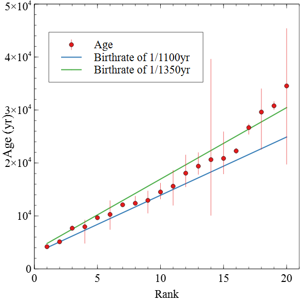
Figure 2: Left panel: Cumulative distribution of model ages from the standard model, and fit lines for birth rates of of 1 per 1200 yr and 1 per 1350 yr. For each parameter of interest (age, energy or density), the sample was sorted in increasing order of parameter to obtain the rank for that parameter. The rise in age with rank for the last 4 SNRs is probably caused by incompleteness. Right panel: Cumulative distributions of s=0, n=7 model explosion energies and of densities of the 20 SNRs. The fit lines are best fit log-normal distributions. For explosion energies the mean is E₀=1.6$\times 10^{51}$ erg and the 1$\sigma$ dispersion in log(E₀) is 0.271 (a factor of 1.87). For densities the mean is $n_{0}$=0.14 cm^-3 and the 1$\sigma$ dispersion in log($n_{0}$) is 0.486 (a factor of 3.06).

We add this SNR to the age distribution and show the age distribution in the left panel of Figure 2. For each parameter of interest (age, energy or density), the sample was sorted in increasing order of parameter to obtain the rank for that parameter. The straight lines are the expected distributions for constant birth rates of 1/(1100 yr) yr and 1/(1350 yr), respectively. The rise in age with rank for the last 4 SNRs is probably caused by incompleteness, which means the true rank (rank if the missing SNRs were included) of those 4 is larger. Thus when we fit for birthrate we omit those 4 from the sample. The lines in Fig. 2 have non-zero x-intercepts of -2.64 and -2.58, respectively.

A birthrate of 1/(1230 yr) line is the best fit to the youngest 16 SNRs of the 20 SNR sample, where the completeness is best, with $\chi^{2}=$10.9 for 14 degrees of freedom. With 2 parameters of interest (slope and intercept of the line) the 95% (2 $\sigma$) confidence interval (e.g Press et al. 2002) on birthrate is 1/(1100 yr) to 1/(1350 yr). The non-zero x-intercept of the fits suggest there are $\sim$2-3 missing young SNRs in our sample. Alternately, the stochastic behaviour of SN explosions could explain the lack of $\sim$2-3 young SNRs.

The cumulative distribution of explosion energies is shown in the right panel of Figure 2. This distribution is consistent with a log-normal distribution. The property that SNR explosion energies follow a log-normal distribution was discovered by Leahy (2017) for LMC SNRs and verified for Galactic SNRs by Leahy & Ranasinghe (2018) and Leahy et al. (2020). Here, the best fit of a cumulative log-normal distribution to the observed cumulative distribution has an average energy (peak of the log-normal) $E_{av}=1.6\times 10^{51}$ erg and dispersion $\sigma_{logE}$=0.265 (a 1-$\sigma$ dispersion factor for $E$ of 1.87).

The right panel of Figure 2 shows the cumulative distribution of ISM densities. This distribution is consistent with a log-normal distribution, similar to that found previously for the LMC and the Galaxy. The best fit cumulative distribution is shown by the solid line. The average density is $n_{0,av}=0.14$ cm^-3 and dispersion is $\sigma_{log(n_{0})}$=0.486 ( a 1-$\sigma$ dispersion factor for $n_{0}$ of 3.06). A log-normal distribution is the natural resulting probability distribution if a physical process is caused by a set of many random processes, where the net physical process depends on the product of the individual processes. Thus both the explosion energy distribution and the ISM density distribution are inferred to be caused by a set of individual processes which act as a product (i.e., in series).

The correlation of observed X-ray luminosity with model parameters (energy, density and age) is shown in Figure 3. The explosion energy and age show no correlation with X-ray luminosity. However the ISM density and luminosity are strongly correlated. This is because the normalization of FS emission depends on its emission measure which scales as square of FS density times emission volume. From Figure 3, the correlation of density ($n_{0}$) on X-ray luminosity ($L_{X}$) follows a $\sim$2/3 powerlaw, so luminosity depends on density as $L_{X}\propto n_{0}^{3/2}$. This is weaker than the expected $n_{0}^{2}$ probably because of other effects. These other effects are seen in the left panel of Figure 1. ISM density is negatively correlated with age and SNR energy is weakly but positively correlated with age. The former is likely caused by the shorter lifetimes of SNRs in high density ISM and could weaken the correlation of X-ray luminosity and density, as seen in Figure 3.

4.1.2 Comparison with LMC and Galactic SNRs

Table 3 compares the results for SNR birthrate, energy and ISM density from the current work with the values for the LMC and the Galaxy from previous work. The birthrates are expected to be different because of the different total stellar masses of SMC, LMC and the Galaxy, and different selection (incompleteness) effects for the three systems. Because the extinction is low for the SMC and LMC the X-ray samples of SNRs are expected to be complete down to a given X-ray luminosity. The incompleteness for the Galaxy is expected to be higher and have strong spatial dependence because of the high extinction in the Galactic plane, particularly for SNRs further from the Sun. An estimage of the observed SNR birthrate for the Galaxy can be obtained by combining the 15 SNR and 43 SNR samples, which have no SNRs in common. The result is an observed birthrate of 1/(236 yr). Correction for selection effects is beyond the scope of the current work. However, this is lower than the SN rate of 1/(40 yr) for our Galaxy, including all types of SN (Tammann et al., 1994), which yields an incompleteness in the 58 SNR sample of a factor $\sim$6.

$E_{av}$ for the SMC SNRs is a factor of 3-4 times larger than the values from the LMC SNR sample or from the two Galactic SNR samples. That the SMC SNR energies are significantly higher is not related to sensitivity of the observations. The LMC is nearer at 50kpc than the SMC at 60kpc so a given flux lower limit results in a luminosity lower limit 1.44 times larger for the SMC. The LMC and SMC surveys did not have a uniform set of exposure times, although the coverage of the SMC survey was significantly more complete than that of the LMC (Maggi et al. 2016,Maggi et al. 2019). However, the faintest SNRs detected in both SMC and LMC have 0.3-8 keV X-ray luminosities of 5-7$\times 10^{33}$erg/s (Filipović et al., 2022). The higher energy may be related to the lower metallicity of the SMC than either the LMC or the Galaxy: lower metallicity stars have weaker stellar winds, thus result in higher stellar mass at the time of explosion for given initial stellar mass. It may also be related to a recent burst of star formation which yielded energetic-SN progenitors.

The mean ISM density of the SMC SNR sample is higher than for the LMC SNRs, and the dispersion is smaller. The lower metallicity of SMC progenitor stars is expected to result in weaker stellar winds, which would lead to an ISM which is less affected by large low density stellar wind bubbles, and thus have a higher mean density and also a lower dispersion in density. Supporting this argument, the dispersion in ISM density for the Galaxy is higher than either SMC or LMC, which is expected from the more inhomogeneous environments in the Galaxy compared to SMC or LMC. Combining the 15 Galactic SNRs in the inner Galaxy (l=18-54^∘) with the 43 Galactic SNRs, we find a mean density of 0.12 cm^-3. The mean density should approximately reflect the density at the mean Galactocentric radius of Galactic SNRs.

4.2 Two-component SNRs

Six of the SNRs (J0049-7314, J0051-7321, J0105-7210, J0104-7201 (=E0102-7219), J0105-7223 and J0106-7205) have two measured X-ray emission components, from forward-shocked (FS) and reverse-shocked (RS) material. For J0104-7201, the whole-SNR hot plasma components are calculated from the sub-regions given by Alan et al. (2019). We applied (s,n)= (0,7), (0,10), (2,6), (2,7), (2,8) and (2,10) models by requiring each model to match the measured FS quantities, $R_{FS}$, $EM_{FS}$ and $kT_{FS}$. The results are shown in Table 2.

Given the assumptions of the SNR models, we assess their ability to reproduce the observed $kT_{RS}$ and $EM_{RS}$ of the SMC SNRs with observed $RS$ properties. The models listed in Table 2 were calculated assuming CC abundances from Leahy & Williams (2017). For CC-type, we use $M_{ej}=5M_{\odot}$; for Ia?-type, we use $M_{ej}=1.4M_{\odot}$. We approximately take into account the effects of ejecta abundances (Ia vs. CC) on $EM_{RS}$ and $kT_{RS}$ using the results of abundance and partial ionization effects from Leahy (2022, in preparation).

Including these effects, the change in $EM_{RS}$ is by factors between 0.01 to 1.5 and the change in $kT_{RS}$ is by factors between 0.1 and 2, with the largest decrease in both $EM_{RS}$ and $kT_{RS}$ caused by changing abundances from CC-type to Ia-type.

4.2.1 Two-component models for individual SNRs

J0049-7314/Ia?: Of the given CC models, (s,n)=(2,8) is closest with $EM_{RS}$ consistent within errors but $kT_{RS}$ too low by factor 0.22. This SNR is Type Ia?, which decreases the model $EM_{RS}$ and $kT_{RS}$ values, making the disagreement worse. The (s,n)=(0,7) model has a Type Ia adjusted $kT_{RS}$ of 0.76$\pm 0.23$ keV, consistent with the data, but far too small $EM_{RS}$. A possibility that this SN has a significant amount of light elements, including hydrogen, mixed in the ejecta, increasing the model $EM_{RS}$, and NEI effects raise the model $kT_{RS}$ to be consistent with the data.

J0051-7321/CC: None of the listed CC models match the data. Model (s,n)=(2,7) has the closest values, a factor 3 to 4 higher (for $EM_{RS}$) and lower (for $kT_{RS}$) than the data. Fewer light elements in the ejecta can lower the model $EM_{RS}$ to match the data, and NEI can raise $kT_{RS}$ to be less discrepant.

J0104-7102/CC: The measured $kT_{RS}$ and $EM_{RS}$ are between those models with (s,n)=(2,7) and (s,n)=(2,8), thus this SNR is consistent with (s,n)=(2,$\sim$7.5).

J0105-7210/Ia?: CC model (s,n)=(2,7) is consistent with both measured $kT_{RS}$ and $EM_{RS}$. However this SNR is classified as Type Ia?, so the model values should be adjusted down and become not consistent with the data. We conclude that this SN may have a significant amount light elements mixed in the ejecta which keeps $kT_{RS}$ and $EM_{RS}$ close to the CC model values.

J0105-7223/CC: CC model (s,n)=(2,7) is the closest one to the measured $kT_{RS}$ and $EM_{RS}$ (within factors of $\sim$1.2), thus this model is consistent with the SNR.

J0106-7205/Ia?: The (s,n)=(2,7) model is the closest one to the measured $kT_{RS}$ and $EM_{RS}$ (within factors of $\sim$1.5). Similar to the case of J0049-7314, this SNR is classified as Type Ia?, so we conclude this SN may have a significant amount light elements mixed in the ejecta.

4.2.2 Discussion of two-component models

Three of the six 2-component SNRs are classified as Ia?, and three as CC. Above we applied a standard set of CC abundances for the composition of the ejecta, which was assumed to be uniformly mixed. Use of uniformly mixed Type Ia abundances, with little hydrogen in the ejecta, yields smaller EM for RS material, because EM is defined in terms of hydrogen abundance. This makes the calculated EM very sensitive to the assumed hydrogen abundance (see Section 4.2). Thus we chose to use CC abundances and estimate the correction to Type Ia abundances after calculating the SNR models. For the three Type Ia? SNRs the SNR type classification might be in in error (Roper et al., 2015). However we think the sensitivity of the EM of RS material to the assumptions of RS composition is more likely what is making the comparison of models with data difficult to interpret.

Two SNRs (J0104-7102/CC and J0105-7223/CC) are well matched by the CC model for $kT_{RS}$ and $EM_{RS}$. For the other four 2-component SNRs, effects of changes in ejecta composition and of partial ionization considered by Leahy (2022, in preparation) are needed to change the model $kT_{RS}$ and $EM_{RS}$ to be consistent with the data. The models are consistent with the three Type Ia SNRs if they have a significant amount of hydrogen mixed into the ejecta. The CC-type SNR J0051-7321 is consistent with the models if the amount of light elements in the ejecta is moderately less than for the standard assumed CC abundances. A possible alternate solution to the $EM_{RS}$ and $kT_{RS}$ discrepancies is to have inhomogeneous ejecta. These effects could be investigated by applying individual complex hydrodynamic solutions including inhomogeneities.

One tentative result is that the best-estimated models for the six two component SNRs are in stellar wind environments rather in uniform density environments. The previous study on Galactic SNRs by Leahy et al. (2020) had a similar conclusion: i.e. most two-component SNRs occur in a circumstellar wind environment. In that study, nine of the twelve two-component SNRs were found to be more consistent with stellar wind environments and only three more consistent with a uniform circumstellar medium. More work on the effects of abundance variations, partial ionization and deviations from spherical symmetry needs to be carried out to verify whether there is a large fraction of two-component SNRs in stellar wind environments. Because SNRs in a stellar wind have significantly larger $EM_{RS}$ than those in a uniform ISM (e.g., see Table 2 here, where the s=2 SNRs have $EM_{RS}$ $\sim$1000 times larger than s=0 SNRs), two-component SNRs should be strongly biased to detection of stellar wind SNRs. This means that the high fraction of stellar wind SNRs in the two-component SNR sample, does not likely extend to the full sample of SNRs.

5 Conclusion

We utilize recent X-ray observations of 20 SNRs in the SMC. The SNR models of (Leahy et al., 2019) are applied to these SNRs with inputs their observed radii, emission measures and temperatures. The models yield explosion energies, circumstellar densities and ages. The distributions of the parameters were used to estimate properties of the SMC SNR population. The energies and ISM densities of SNRs can be well fit with log-normal distributions in agreement with our earlier studies (Leahy 2017, Leahy & Ranasinghe 2018, Leahy et al. 2020). The mean density of SNR environments in the SMC is 0.1 cm^-3. The mean explosion energy is $1.6\times 10^{51}$ erg, which is significantly higher than the mean energy of LMC SNRs ($\simeq 5\times 10^{50}$ erg or of Galactic SNRs $\simeq 4\times 10^{50}$). The derived birthrate of SMC SNRs is $\simeq$1 per 1200 yr

Six of the 20 SNRs have two component X-ray spectra, i.e. both forward shocked material and reverse shocked ejecta are detected. We apply different (s,n) models to these SNRs and conclude that other effects not built into the SNR models must be important for the models to match both forward shock and reverse shock properties. These effects include changes in ejecta composition and partial ionization, discussed quantitatively by Leahy (2022, in preparation). By accounting for these effects, the best models for these SNRs are likely models for a SNR in a stellar wind environment. Further exploration of two-component SNRs requires more complex model calculations which include the effects above or non-spherical models.

Figure 3: Standard model energy, density and age vs. observed X-ray luminosity for the 20 SNRs.

Table 1: All SNRs: Standard (s=0, n=7 forward shock) Model Results

SNR	SN type	$M_{ej}$	Age(+.-)	Energy(+,-)	Density(+,-)
		($M_{\odot}$)	(kyr)	($10^{50}$ erg)	($10^{-2}$ cm-3)
J0041-7336	CC	5	19.4(+2.6,-1.6)	23.6(+4.4,-5.3)	6.1(+0.7,-0.3)
J0046-7308	CC	5	14.5(+1.7,-1.4)	16.3(+3.5,-3.3)	14.6(+3.0,-1.7)
J0047-7308	CC	5	9.7(+0.5,-0.3)	11.2(+1.8,-1.0)	36.6(+6.1,-0.6)
J0047-7309	CC	5	12.9(+1.8,-2.5)	13.0(+6.8,-7.2)	14.2(+5.3,-8.7)
J0048-7319	unknown	1.4	8.0(+1.3,-3.2)	14.2(+24.9,-3.8)	6.1(+1.7,-2.1)
J0049-7314	Ia?	1.4	18.1(+3.5,-2.6)	11.5(+4.7,-3.4)	7.3(+3.3,-2.2)
J0051-7321	CC	5	22.3(+0.6,-0.5)	21.4(+1.3,-2.1)	79.6(+4.9,-8.1)
J0052-7236	CC	5	34.5(+10.9,-14.8)	46.7(+114.0,-30.8)	10.5(+25.5 ,-7.1)
J0056-7209	unknown	1.4	20.6(+19.0,-10.6)	22.4(+71.7,-16.3)	2.8(+2.6,-0.9)
J0057-7211	unknown	1.4	10.3(+2.6,-2.9)	12.3(+11.5,-4.5)	5.5(+0.7,-0.8)
J0058-7217	CC	5	29.6(+4.4,-7.1)	36.2(+27.0,-18.4)	13.9(+10.4,-7.2)
J0059-7210	CC	5	12.1(+0.3,-0.3)	25.9(+1.3,-1.2)	33.1(+1.5,-1.4)
J0100-7133	CC	5	20.9(+5.1,-3.0)	13.1(+7.0,-4.6)	6.4(+3.8,-1.1)
J0103-7209	CC	5	15.6(+3.1,-3.6)	43.3(+30.4,-13.0)	3.4(+0.4,-0.4)
J0103-7247	CC	5	5.1(+0.4,-0.3)	8.7(+1.4,-1.4)	10.6(+2.6,-2.4)
J0104-7201a	CC	5	4.2(+0.1,-0.3)	7.2(+1.2,-0.8)	338(+43,-40)
J0105-7210	Ia?	1.4	12.4(+1.4,-0.2)	13.1(+2.0,-2.5)	12.2(+2.1,-1.1)
J0105-7223	CC	5	30.8(+0.8,-0.8)	47.0(+2.6,-2.8)	83.0(+4.6,-4.8)
J0106-7205	Ia?	1.4	7.7(+0.5,-0.4)	9.8(+1.1,-1.2)	37.5(+2.8,-3.0)
J0127-7333	unknown	1.4	26.7(+0.7,-1.3)	9.1(+2.9,-2.6)	25.0(+7.8,-7.1)

Table 2: SNRs with Two Components: Predicted Reverse Shock Properties

SNR/Typea	s,n	Age(+.-)	Energy(+,-)	$n_{-2}$(+,-) or $\rho_{s,14}$(+,-)	$kT_{r}$(+,-)	$EM_{r}$(+,-)
		(kyr)	($10^{50}$erg)	($10^{-2}$ cm-3 or	(keV)	($10^{56}$cm-3)
				$10^{13}M_{\odot}$s/(km yr))
J0049-7314/Ia? Observed		n/a	n/a	n/a	0.91(0.03,-0.03)	728(+125,-99)
J0049-7314 Models	0,7	18.1(+3.5,-2.6)	11.5(+4.7,-3.4)	$n_{-2}$=7.3(+3.3,-2.2)	3.6(1.1,-1.0)	0.11(+0.02,-0.02)
	0,10	17.9(+3.4,-2.6)	11.7(+4.9,-3.4)	$n_{-2}$=7.3(+3.3,-2.2)	2.2(+0.6,-0.6)	0.19(+0.03,-0.03)
	2,6	6.6(+2.5,-1.5)	38(+26,-18)	$\rho_{s,14}$=2.05(+0.95,-0.63)	0.18(+0.05,-0.05)	156(+180,-81)
	2,7	1.63(+0.38,-0.24)	218(+82,-74)	$\rho_{s,14}$=0.86(+0.40,-0.26)	0.55(+0.16,-0.15)	102(+117,-53)
	2,8	2.65(+0.77,-0.46)	66(+30,-26)	$\rho_{s,14}$=1.14(+0.53,-0.35)	0.20(+0.06,-0.05)	430(+490,-220)
	2,10	2.70(+0.78,-0.46)	38(+17,-15)	$\rho_{s,14}$=1.08(+0.50,-0.33)	0.11(+0.03,-0.03)	1300(+1500,-700)
J0051-7321/CC Observed		n/a	n/a	n/a	0.73(0.16,-0.10)	1240(+526,-215)
J0051-7321 Models	0,7	22.3(+0.6,-0.5)	21.4(+1.3,-2.1)	$n_{-2}$=79.6(+4.9,-8.1)	1.74(+0.08,-0.10)	3.60(+0.09,-0.16)
	0,10	22.1(+0.6,-0.5)	21.9(+1.4,-2.2)	$n_{-2}$=79.6(+5.0,-8.1)	1.08(+0.05,-0.07)	6.16(+0.16,-0.27)
	2,6	13.7(+0.4,-0.3)	22.9(+1.2,-1.5)	$\rho_{s,14}$=13.2(+0.8,-1.4)	0.072(+0.003,-0.003)	8500(+1100,-1700)
	2,7	3.89(+0.20,-0.19)	93(+9,-9)	$\rho_{s,14}$=5.5(+0.4,-0.6)	0.22(+0.01,-0.01)	5500(+700,-1200)
	2,8	7.61(+0.32,-0.29)	18.7(+1.5,-1.5)	$\rho_{s,14}$=7.32(+0.46,-0.76)	0.080(+0.004,-0.004)	23400(+3100,-4600)
	2,10	7.74(+0.33,-0.30)	10.5(+0.9,-0.8)	$\rho_{s,14}$=6.94(+0.44,-0.72)	0.043(+0.002,-0.002)	71000(+9000,-14000)
J0104-7201/CC Observed		n/a	n/a	n/a	0.62(0.10,-0.10)	8100(+800,-800)
J0104-7201 Models	0,7	4.19(+0.08,-0.32)	7.2(+1.2,-0.8)	$n_{-2}$=338(+43,-40)	1.03(+0.17,-0.11)	40.4(+5.6,-4.5)
	0,10	4.15(+0.08,-0.31)	7.3(+1.3,-0.8)	$n_{-2}$=339(+44,-41)	0.58(+0.12,-0.11)	61.2(+9.7,-8.9)
	2,6	2.22(+0.06,-0.25)	18.8(+5.2,-0.9)	$\rho_{s,14}$=5.12(+0.64,-0.50)	0.200(+0.035,-0.007)	4270(+1240,-860)
	2,7	0.461(+0.014,-0.058)	206(+64,-12)	$\rho_{s,14}$=2.15(+0.27,-0.25)	0.604(+0.105,-0.021)	2800(+740,-620)
	2,8	0.909(+0.029,-0.127)	50.3(+19.5,-3.5)	$\rho_{s,14}$=2.85(+0.35,-0.34)	0.223(+0.039,-0.008)	11800(+3200,-2600)
	2,10	0.921(+0.034,-0.138)	36.3(+14.0,-2.5)	$\rho_{s,14}$=2.71(+0.34,-0.32)	0.121(+0.021,-0.004)	36200(+9700,-8000)
J0105-7210/Ia? Observed		n/a	n/a	n/a	0.78(0.07,-0.30)	188(+63,-58)
J0105-7210 Models	0,7	12.4(+1.4,-0.2)	13.1(+2.0,-2.5)	$n_{-2}$=12.2(+2.1,-1.1)	4.30(0.41,-0.70)	0.20(+0.01,-0.01)
	0,10	12.3(+1.4,-0.2)	13.3(+2.0,-2.5)	$n_{-2}$=12.2(+2.1,-1.1)	2.64(+0.26,-0.43)	0.35(+0.02,-0.01)
	2,6	4.28(+0.86,-0.13)	51.0(+3.2,-15.6)	$\rho_{s,14}$=2.16(+0.38,-0.20)	0.241(+0.007,-0.040)	220(+85,-39)
	2,7	1.11(+0.13,-0.02)	270(+17,-54)	$\rho_{s,14}$=0.91(+0.16,-0.08)	0.72(+0.02,-0.12)	143(+55,-25)
	2,8	1.78(+0.26,-0.04)	85.2(+3.8,-20.2)	$\rho_{s,14}$=1.20(+0.20,-0.11)	0.264(+0.008,-0.043)	608(+236,-107)
	2,10	1.81(+0.26,-0.04)	50.2(+2.2,-11.8)	$\rho_{s,14}$=1.14(+0.20,-0.11)	0.144(+0.004,-0.023)	1850(+710,-330)
J0105-7223/CC Observed		n/a	n/a	n/a	0.38(0.01,-0.01)	8530(+2630,-2070)
J0105-7223 Models	0,7	30.8(+0.8,-0.8)	47.0(+2.6,-2.8)	$n_{-2}$=83.0(+4.6,-4.8)	2.66(+0.14,-0.14)	2.23(+0.05,-0.05)
	0,10	30.6(+0.8,-0.8)	48.1(+2.7,-2.8)	$n_{-2}$=83.1(+4.6,-4.9)	1.65(+0.09,-0.09)	3.81(+0.08,-0.09)
	2,6	19.2(+0.5,-0.5)	37.4(+2.0,-2.0)	$\rho_{s,14}$=24.5(+1.4,-1.5)	0.065(+0.003,-0.003)	22200(+2600,-2600)
	2,7	6.24(+0.34,-0.31)	100(+11,-10)	$\rho_{s,14}$=10.3(+0.6,-0.6)	0.20(+0.01,-0.01)	14400(+1700,-1700)
	2,8	11.50(+0.47,-0.44)	20.6(+1.7,-1.6)	$\rho_{s,14}$=13.6(+0.8,-0.8)	0.071(+0.004,-0.004)	61300(+7100,-7100)
	2,10	11.7(+0.5,-0.5)	10.4(+0.9,-0.8)	$\rho_{s,14}$=12.9(+0.7,-0.8)	0.039(+0.002,-0.002)	1.8$\times 10^{5}$(+2$\times 10^{4}$,-2$\times 10^{4}$)
J0106-7205/Ia Observed		n/a	n/a	n/a	1.00(0.03,-0.03)	788(+103,-95)
J0106-7205/Ia Models	0,7	7.7(+ 0.5,-0.4)	9.8(+1.1,-1.2)	$n_{-2}$=37.5(+2.8,-3.0)	3.83(+0.38,-0.42)	0.74(0.03,-0.03)
	0,10	7.6(+0.5,-0.4)	9.9(+1.1,-1.2)	$n_{-2}$=37.4(+2.8,-2.9)	2.35(+0.23,-0.26)	1.28(+0.04,-0.04)
	2,6	2.97(+0.37,-0.27)	33.2(+7.0,-7.0)	$\rho_{s,14}$=2.55(+0.20,-0.20)	0.254(+0.025,-0.029)	492(+79,-75)
	2,7	0.70(+0.06,-0.04)	227(+29,-33)	$\rho_{s,14}$=1.07(+0.08,-0.08)	0.76(+0.07,-0.08)	320(+51,-49)
	2,8	1.16(+0.12,-0.08)	69(+11,-12)	$\rho_{s,14}$=1.42(+0.11,-0.11)	0.280(+0.027,-0.031)	1360(+220,-210)
	2,10	1.18(+0.12,-0.08)	42.2(+6.7,-7.4)	$\rho_{s,14}$=1.35(+0.10,-0.11)	0.153(+0.015,-0.017)	4140(+660,-630)

Table 3: Comparison of SMC, LMC and Galactic SNR Rates, Energies and Densities

System	Mean SNR Rate	2$\sigma$ Rate Range	Mean Energy	1$\sigma$ Energy Dispersion	Density	1$\sigma$ Density Dispersion
	(1/yr)	(1/yr)	($10^{51}$ erg)	(ratio)	( cm-3)	(ratio)
SMC 20 SNRsa	1230	1100-1350	1.6	1.87	0.14	3.06
LMC 50 SNRsb	503	490-525	0.48	2.94	0.079	3.24
Galaxy 15 SNRs (l=18-54∘)c	870	740-1000	0.54	3.47	0.26	6.31
Galaxy 43 SNRs (l=38-360∘)d	324	302-347	0.27	3.47	0.069	5.13

References

- Alan et al. (2019) Alan, N., Park, S., & Bilir, S. 2019, ApJ, 873, 53. doi:10.3847/1538-4357/aaf882
- Badenes et al. (2006) Badenes, C., Borkowski, K. J., Hughes, J. P., et al. 2006, ApJ, 645, 1373. doi:10.1086/504399
- Banovetz et al. (2021) Banovetz, J., Milisavljevic, D., Sravan, N., et al. 2021, ApJ, 912, 33. doi:10.3847/1538-4357/abe2a7
- Chevalier (1982) Chevalier, R. A. 1982, ApJ, 258, 790
- Chevalier (1982) Chevalier, R. A. 1982, ApJ, 259, 302. doi:10.1086/160167
- Cioffi et al. (1988) Cioffi, D. F., McKee, C. F., & Bertschinger, E. 1988, ApJ, 334, 252
- Colgate & McKee (1969) Colgate, S. A. & McKee, C. 1969, ApJ, 157, 623. doi:10.1086/150102
- Cox (2005) Cox, D. P. 2005, ARA&A, 43, 337
- Dickey & Lockman (1990) Dickey, J. M. & Lockman, F. J. 1990, ARA&A, 28, 215. doi:10.1146/annurev.aa.28.090190.001243
- Filipović et al. (2022) Filipović, M. D., Payne, J. L., Alsaberi, R. Z. E., et al. 2022, arXiv:2201.10026
- Graczyk et al. (2014) Graczyk, D., Pietrzyński, G., Thompson, I. B., et al. 2014, ApJ, 780, 59. doi:10.1088/0004-637X/780/1/59
- Hilditch et al. (2005) Hilditch, R. W., Howarth, I. D., & Harries, T. J. 2005, MNRAS, 357, 304. doi:10.1111/j.1365-2966.2005.08653.x
- Leahy (2017) Leahy, D. A. 2017, ApJ, 837, 36
- Leahy & Williams (2017) Leahy, D. A., & Williams, J. E. 2017, AJ, 153, 239
- Leahy & Ranasinghe (2018) Leahy, D. A., & Ranasinghe, S. 2018, ApJ, 866, 9
- Leahy et al. (2019) Leahy, D., Wang, Y., Lawton, B., et al. 2019, AJ, 158, 149
- Leahy et al. (2020) Leahy, D. A., Ranasinghe, S., & Gelowitz, M. 2020, ApJS, 248, 16. doi:10.3847/1538-4365/ab8bd9
- Long et al. (2020) Long, X., Gaetz, T. J., & Plucinsky, P. P. 2020, ApJ, 904, 70. doi:10.3847/1538-4357/abc075
- Maggi et al. (2016) Maggi, P., Haberl, F., Kavanagh, P. J., et al. 2016, A&A, 585, A162. doi:10.1051/0004-6361/201526932
- Maggi et al. (2019) Maggi, P., Filipović, M. D., Vukotić, B., et al. 2019, A&A, 631, A127. doi:10.1051/0004-6361/201936583
- Nadezhin (1985) Nadezhin, D. K. 1985, Ap&SS, 112, 225
- Pietrzyński et al. (2019) Pietrzyński, G., Graczyk, D., Gallenne, A., et al. 2019, Nature, 567, 200. doi:10.1038/s41586-019-0999-4
- Press et al. (2002) Press, W. H., Teukolsky, S. A., Vetterling, W. T., et al. 2002, Numerical recipes in C++ : the art of scientific computing by William H. Press. xxviii, 1,002 p. : ill. ; 26 cm. Includes bibliographical references and index. ISBN : 0521750334
- Rasmussen et al. (2001) Rasmussen, A. P., Behar, E., Kahn, S. M., et al. 2001, A&A, 365, L231. doi:10.1051/0004-6361:20000231
- Roper et al. (2015) Roper, Q., McEntaffer, R. L., DeRoo, C., et al. 2015, ApJ, 803, 106. doi:10.1088/0004-637X/803/2/106
- Sasaki et al. (2001) Sasaki, M., Stadlbauer, T. F. X., Haberl, F., et al. 2001, A&A, 365, L237. doi:10.1051/0004-6361:20000015
- Tammann et al. (1994) Tammann, G. A., Loeffler, W., & Schroeder, A. 1994, ApJS, 92, 487
- Truelove & McKee (1999) Truelove, J. K., & McKee, C. F. 1999, ApJS, 120, 299
- Vink (2012) Vink, J. 2012, A&A Rev., 20, 49