Stable Charged Gravastar Model in ${f}(\mathfrak{R},\textbf{T}^{2})$ Gravity with Conformal Motion

Abstract

This paper investigates the influence of charge on physical features of gravastars in the framework of energy-momentum squared gravity. A gravastar is an alternate model to a black hole that comprises of three distinct regions, namely the intermediate shell, inner and outer sectors. Different values of the barotropic equation of state parameter provide the mathematical formulation for these regions. We construct the structure of a gravastar admitting conformal motion for a specific model of energy-momentum squared gravity. The field equations are formulated for a spherically symmetric spacetime with charged perfect matter distribution. For the smooth matching of external and internal spacetimes, we use Israel matching criteria. Various physical attributes of gravastars such as the equation of state parameter, proper length, entropy and energy are investigated (in the presence of charge) versus thickness of the shell. The charge in the inner core of gravastars preserves the state of equilibrium by counterbalancing the inward gravitational force. It is concluded that the non-singular solutions of charged gravastar are physically viable in the background of energy-momentum squared gravity.

Keywords: Gravastars; Modified theories; Israel formalism.
PACS: 04.50.Kd; 04.70.Dy; 97.10.Cv.

1 Introduction

The study of the incredibly huge cosmos gives insight into its mysterious nature. Recent cosmic observations such as supernova type 1a, cosmic microwave background radiations as well as large-scale structures indicate that the cosmos is expanding at a rapid rate [1]. The unknown strange force responsible for this expansion is dubbed as dark energy. Although the general theory of relativity (GR) provides a platform for the discussion of cosmic issues, it fails to explain the accelerated expansion of the universe due to the well-known problems: fine-tuning and cosmic coincidence. Moreover, the occurrence of singularities in GR is a crucial problem as they are predicted in the regime of high-energy where GR is not applicable due to quantum effects. Based on these issues, different modifications of GR have been proposed to study the singularity problem as well as to investigate the attributes of mysterious dark energy. A natural extension of GR, known as $f(\mathfrak{R})$ gravity, is obtained by including the associated function of curvature invariant $(\mathfrak{R})$ in the geometric sector of the Einstein-Hilbert action. Different cosmological and astrophysical problems have been successfully addressed in this theory [2].

Harko et al. [3] introduced $f(\mathfrak{R},T)$ gravity as a generalization of $f(\mathfrak{R})$ theory by including the trace of energy-momentum tensor (EMT) $T$. Haghani et al. [4] incorporated the contraction of Ricci scalar and EMT $({\mathfrak{R}}_{\mu\nu}{T}^{\mu\nu})$ in $f(\mathfrak{R},T)$ gravity to analyze the effect of non-linear correction terms appearing due to the non-minimal coupling between curvature and matter. These theories disobey the conservation law which proves the existence of an additional force acting on particles. Thus, under the influence of this force, the motion of particles is non-geodesic. These theories have captivated the attention of many researchers as the minimal/non-minimal interaction of matter and curvature is thought to be a good fit for comprehending the the connection between rapid expansion and dark cosmic components. Moreover, these couplings efficiently describe the rotation curves of galaxies and distinct cosmic ages of the cosmos.

The beginning of the cosmos presents an interesting problem for cosmologists. In this regard, different researchers have tried to formulate adequate cosmic models explaining the evolution of the universe since the advent of time. According to the big-bang theory, matter and energy of the cosmos were initially concentrated at a single point (known as a singularity) having limitless density and temperature with no surface area or volume. The universe came into existence due to the explosion of superheated ultra-dense matter within the singularity and has been expanding since then. Big bounce theory is an alternative approach describing the evolution of the cosmos as a series of big bounces (expanding and contracting over and over again) having no beginning or end state. In this regard, energy-momentum squared gravity (EMSG) [5] has been proposed which favors the big bounce theory. It modifies the Einstein-Hilbert action by including the analytic function of the form ${T}_{\mu\nu}{T}^{\mu\nu}=\textbf{T}^{2}$. In the perspective of this theory, the cosmos with maximum energy density as well as a minimum-scale factor in the early epoch bounces to a state of expansion [6]. Consequently, this theory resolves the big-bang singularity in non-quantum prescription without affecting cosmic evolution.

The quadratic components of matter source in EMSG field equations help in resolving fascinating cosmological and astrophysical issues. In the context of the standard cosmological model, the cosmological constant does not play an important role in the early times and becomes important only after the matter-dominated era. Roshan and Shojai [6] found that in this theory, the repulsive nature of the cosmological constant plays a crucial role at early times in resolving the singularity. Moreover, it has been shown that this theory possesses a true sequence of cosmological eras. Board and Barrow [7] found isotropically expanding cosmos for matter theories of higher-order. Nari and Roshan [8] determined the existence of pressureless compact stars in EMSG and obtained stellar models that are less compact in comparison to their GR counterparts. Akarsu et al. [9] discussed the modification of the $\Lambda$CDM model. They investigated the non-minimal interactions for relativistic compact objects and dark matter in the context of EMSG and have obtained suitable constraints on the model. Moraes and Sahoo [10] studied the geometry of non-exotic wormholes. Bahamonde et al. [11] presented the expansion of cosmos using different coupling models and found that these models are a good fit to explain the current behavior of cosmos. Sharif and Gul [12] used Noether symmetries in this theory and studied the impact of different physical parameters on viable cosmological structures. They also inspected the viability as well as stability of compact celestial bodies and concluded that the correction terms of the gravity decrease the collapse.

Different astrophysical phenomena, such as the development and evolution of stellar structures have sparked the interest of different researchers. Among all the cosmic entities, stars are the core components of galaxies, which are arranged systematically in a cosmic web. The outward pressure in a star vanishes when it exhausts its fuel. Consequently, the star undergoes gravitational collapse which leads to the formation of compact objects. One of the stellar remnants is a black hole which is a completely collapsed object with a singularity covered by an event horizon. In order to overcome singularity and event horizon problems, Mazur and Motolla [13] proposed a cold compact model (referred to as gravitationally vacuum star or gravastar) as an alternative to the black hole. The most crucial feature of this hypothetical object is its singularity-free nature in contrast to the black hole. It comprises of three regions: the interior and exterior regions are separated by an intermediate thin-shell. The singularity is avoided by considering the de Sitter (dS) spacetime in the innermost region with a surrounding layer of cold baryonic fluid that separates the inner and outer regions, whereas the exterior vacuum is described by the Schwarzschild metric. Moreover, each sector is characterized by a particular equation of state (EoS).

There is currently no observational evidence in support of gravastar, however, a few indirect evidences in literature can be used to predict gravastar’s occurrence and future detection. Sakai et al. [14] presented a mechanism to detect gravastar through the exploration of gravastar shadows. Gravitational lensing is another possible approach for detecting gravastars, as hypothesized by Kubo and Sakai [15], who claimed that microlensing effects of maximal luminosity do not occur in black holes. However, these effects can be observed in gravastar having the same mass as that of black hole. The detection of GW150914 through interferometric LIGO detectors [16]-[17], hinted towards the presence of ringdown signal generated by objects without an event horizon. A recent analysis of the image acquired by the First M87 Event Horizon Telescope (EHT) suggests a shadow that could belong to a gravastar [18].

Visser and Wiltshire [19] inspected the stability of gravastars against radial perturbations and found that the use of feasible EoS leads to stability of gravastar in GR. Carter [20] extended this work by analyzing suitable constraints for the stability of non-singular exact solutions of gravastars. Catteon et al. [21] investigated the usual structure of gravastars and found that the configuration possesses anisotropy in the absence of shell. Bilic et al. [22] constructed solutions of gravatars by using inner Born-Infeld phantom spacetime in place of dS geometry and formulated solutions representing compact objects at the core of galaxies. Horvat and Ilijić [23] examined the stability of the gravastar by applying the speed of sound criterion on the shell and obtained surface compactness bounds. Ghosh et al. [24] showed that the extension of 4-dimensional gravastar to higher dimensions is not possible. Researchers have also investigated the existence and important physical features of gavastars in the context of modified theories of gravity [25]-[28].

Conformal symmetry describes the inherent symmetry of Killing vectors. Mathematically, it is given in the form

$$L_{\varsigma}g_{mn}=\Phi(r)g_{mn},$$

where the operator $L_{\varsigma}$ describes the Lie derivative, $\Phi$ is the conformal factor and $\varsigma$ denotes a four-vector. The conformal Killing vectors reduce highly nonlinear field equations to linear ordinary differential equations. Herrera and Leon [29] used exact solutions corresponding to spherically symmetric spacetime and found a parametric group of conformal motions. Banerjee et al. [30] investigated various attributes of a braneworld gravastar that allowed conformal motion.

Electromagnetism plays a crucial role in the study of the evolution as well as stability of collapsing objects. A star requires an immense amount of charge to counterbalance the inward pull of gravity and sustain its equilibrium state. Lobo and Arellano [31] studied gravastar solutions incorporating nonlinear electrodynamics and examined significant structural attributes. Horvat et al. [32] investigated charged gravastar and calculated surface redshift, sound speed as well as the EoS parameter for the model under consideration. Turimov et al. [33] presented a brief discussion on slowly rotating gravastars filled with highly magnetized perfect matter. Usmani et al. [34] used conformal motion to compute gravastar models with charged interior and Reissner-Nordström as the exterior. They concluded that the charged interior region acts as an electromagnetic mass model which generates gravitational mass thus contributing to the stability of the gravastar structure. Rahaman et al. [35] studied numerous viable features for gravastar structures in 3-dimensional spacetime with the contribution of charge. Sharif and Javed [36] investigated the stable configuration of gravastars by considering quintessence as well as regular black hole geometries in the interior and observed linear profiles of physical variables versus the thickness of the shell.

In the background of $f(\mathfrak{R},T)$ gravity, Sharif and Waseem [37] investigated charged gravastar structure using conformal motion and found that the inner sector behaves as an electromagnetic mass model in the presence of charge which helps in the formation of singularity-free structure. Bhatti et al. [38] explored the stability of charged gravastar in the modified gravity. Bhar and Rej [39] studied gravastar admitting conformal motion to analyze the contribution of charge to the stability region for the discussed model. Bhatti and his collaborators [40] also studied gravastar structure in the context of ${f(\mathcal{G})}$ gravity, where $\mathcal{G}$ is Gauss-Bonnet invariant. They investigated different attributes of gravastar with and without electromagnetic field. Various attributes of gravastar solutions are also analyzed through the gravitational decoupling technique in [41]. Sharif and Naz [42] studied gravastar structure with Kuchowicz metric in ${f}(\mathfrak{R},\textbf{T}^{2})$ gravity. Recently, Sharif and Saeed [43] studied charge-free gravastar accepting conformal motion in background of $f(\mathfrak{R},\textbf{T}^{2})$ gravity and discussed the behavior of various physical attributes. Motivated by numerous works presenting effects of charge, we are interested to analyze the influence of charge on the gravastar model in $f(\mathfrak{R},\textbf{T}^{2})$ gravity.

In the present work, we examine the gravastar configuration admitting conformal motion for charged spherical static system in $f(\mathfrak{R},\textbf{T}^{2})$ gravity. The paper is organized according to the following outline. Section 2 describes the framework of $f(\mathfrak{R},\textbf{T}^{2})$ gravity and presents field equations with conformal motion. In section 3, we investigate three distinct regions of gravastar with different EoS. Section 4 includes the discussion of physical attributes of gravastar, i.e., EoS parameter, proper length, entropy and energy of the shell. The last section concludes the major findings of the work.

2 Basic Formalism of $f(\mathfrak{R},\textbf{T}^{2})$ Theory

In this section, we develop the field equations of $f(\mathfrak{R},\textbf{T}^{2})$ theory and conformal equations for charged isotropic matter distribution. The action of this theory is described as [5]

$$\mathcal{I}=\frac{1}{2\kappa^{2}}\int d^{4}x\left[f\left(\mathfrak{R},{\textbf{T}}^{2}\right)+\mathcal{L}_{e}+\mathcal{L}_{m}\right]{\sqrt{-g}},$$ (1)

where $g$ indicates the determinant of the metric tensor, $\mathcal{L}_{m}$ symbolizes the matter Lagrangian and $\kappa^{2}=1$ is a coupling constant. Furthermore, $\mathcal{L}_{e}=\frac{-1}{16\pi}\mathcal{F}^{\mu\nu}\mathcal{F}_{\mu\nu}$ where $\mathcal{F}_{\mu\nu}=\varphi_{\nu,\mu}-\varphi_{\mu,\nu}$ describes the electromagnetic field tensor and $\varphi_{\mu}$ represents the four potential. The respective field equations turn out to be

$$\mathfrak{R}_{\mu\nu}f_{\mathfrak{R}}-\frac{1}{2}g_{\mu\nu}f+g_{\mu\nu}\Box f_{\mathfrak{R}}-\nabla_{\mu}\nabla_{\nu}f_{\mathfrak{R}}=T_{\mu\nu}-\Theta_{\mu\nu}f_{\textbf{T}^{2}}+\mathrm{E}_{\mu\nu},$$ (2)

where $f\equiv f(\mathfrak{R},\textbf{T}^{2})$,$~{}\Box={\nabla_{\mu}\nabla^{\mu}},~{}f_{\mathbf{T}^{2}}=\frac{\partial f}{\partial\textbf{T}^{2}},f_{\mathfrak{R}}=\frac{\partial f}{\partial\mathfrak{R}}$,

$$\Theta_{\mu\nu}=-4\frac{\partial^{2}\mathcal{L}_{m}}{\partial g^{\mu\nu}\partial g^{\theta\eta}}T^{\theta\eta}-2\mathcal{L}_{m}\left(T_{\mu\nu}-\frac{1}{2}g_{\mu\nu}T\right)-TT_{\mu\nu}+2T_{\mu}^{\theta}T_{\nu\theta},$$ (3)

and the electromagnetized energy-momentum tensor $\mathrm{E}_{\mu\nu}$ is provided by

$$\mathrm{E}_{\mu\nu}=\frac{1}{4\pi}\left(\mathcal{F}^{\theta}_{\mu}\mathcal{F}_{\nu\theta}-\frac{1}{4}g_{\mu\nu}\mathcal{F}^{\theta\eta}\mathcal{F}_{\theta\eta}\right).$$ (4)

Non-conserved EMT is generated by $f(\mathfrak{R},\textbf{T}^{2})$ gravity, implying the existence of an additional force that describes non-geodesic motion of particles as follows

$$\nabla^{\mu}T_{\mu\nu}=\frac{1}{2}\left[-f_{\mathbf{T}^{2}}g_{\mu\nu}{\nabla^{\mu}}{\mathbf{T}^{2}}+2{\nabla^{\mu}}(f_{\mathbf{T}^{2}}{\Theta_{\mu\nu}})+\nabla^{\mu}\mathrm{E}_{\mu\nu}\right].$$ (5)

In gravitational physics, the EMT describes the energy and matter distribution, where the non-vanishing components provide physical variables that describe various dynamical properties.

We consider isotropic matter configuration

$$T_{\mu\nu}=v_{\mu}v_{\nu}(\mathcal{P}+\varrho)-\mathcal{P}g_{\mu\nu},$$ (6)

where $v_{\mu}$, $\varrho$ and $\mathcal{P}$ define the four-velocity, energy density and pressure of the fluid, respectively. For matter configuration, there are two choices of $\mathcal{L}_{m}$, i.e., either $\mathcal{L}_{m}=\mathcal{P}$, or $\mathcal{L}_{m}=-\varrho$. For theories possessing minimal interaction, matter lagrangian choice does not influence the distribution [44]. Here, we consider $\mathcal{L}_{m}=\mathcal{P}$ and utilizing Eqs.(3) and (6), we have

$$\Theta_{\mu\nu}=-\left(\varrho^{2}+3\mathcal{P}^{2}+4\mathcal{P}\varrho\right)v_{\mu}v_{\nu}.$$

The field equations (2) are complex as well as non-linear in the framework of multivariate functions and their differentials. Therefore, we choose a particular function that demonstrates minimal/non-minimal interactions among geometry and matter components. The field equations corresponding to the non-minimal model turn out to be very complex making the solution of these equations more challenging. Thus, we choose a minimal model for our analysis [5]

$$f(\mathfrak{R},\textbf{T}^{2})=\mathfrak{R}+\beta\textbf{T}^{2},$$ (7)

where $\mathbf{T}^{2}=\varrho^{2}+3\mathcal{P}^{2}$ and $\beta$ is the model parameter. It describes the current accelerated expansion and cosmic evolution of the cosmos. Incorporating $\textbf{T}^{2}$ into this modified gravity results in a wider form of GR than $f(\mathfrak{R})$ and $f(\mathfrak{R},T)$ theories. The functional form (7) explains the $\Lambda$CDM model and has frequently been used to investigate different aspects of self-gravitating objects. It solves a variety of cosmological problems [45] and corresponds to three major epochs of the universe, i.e., dS-dominated, radiation-dominated and matter-dominated era. Plugging this model in Eq.(2), we have

$$\mathbb{G}_{\mu\nu}=T_{\mu\nu}+\frac{1}{2}\beta g_{\mu\nu}{\textbf{T}}^{2}-\beta f_{{\textbf{T}}^{2}}{\Theta_{\mu\nu}}+\mathrm{E}_{\mu\nu},$$ (8)

where $\mathbb{G}_{\mu\nu}$ is the Einstein tensor. We choose static spherically symmetric geometry to examine the interior region of the charged gravastar as

$$ds^{2}=e^{\chi(r)}dt^{2}-e^{\lambda(r)}dr^{2}-r^{2}(d\theta^{2}+\sin^{2}\theta d\phi^{2}).$$ (9)

The associated field equations are

$$\left[-\frac{e^{-\lambda}}{r^{2}}+\frac{1}{r^{2}}+\frac{\lambda^{{}^{\prime}}e^{-\lambda}}{r}\right]=\varrho+\frac{3}{2}\beta\varrho^{2}+\frac{9}{2}\beta\mathcal{P}^{2}+4\beta\varrho\mathcal{P}+\frac{{q}^{2}}{{8\pi{r}^{4}}},$$

$$\left[e^{-\lambda}\left(\frac{1}{r^{2}}+\frac{\chi^{{}^{\prime}}}{r}\right)-\frac{1}{r^{2}}\right]=\mathcal{P}-\frac{\beta}{2}\varrho^{2}-\frac{3}{2}\beta\mathcal{P}^{2}-\frac{{q}^{2}}{{8\pi{r}^{4}}},$$

$$\left[e^{-\lambda}\left(\frac{\chi^{{}^{\prime}2}}{4}+\frac{\chi^{{}^{\prime}}}{2r}-\frac{\lambda^{{}^{\prime}}}{2r}+\frac{\chi^{{}^{\prime\prime}}}{2}-\frac{\chi^{{}^{\prime}}\lambda^{{}^{\prime}}}{4}\right)\right]=\mathcal{P}-\frac{\beta}{2}\varrho^{2}-\frac{3}{2}\beta\mathcal{P}^{2}+\frac{{q}^{2}}{{8\pi{r}^{4}}},$$

(12)

where prime corresponds to the radial derivative.

The conformal killing vectors are obtained by using conformal symmetry which is defined as

$$L_{\varsigma}g_{mn}=g_{jn}\varsigma^{j}_{;m}+g_{mj}\varsigma^{j}_{;n}=\Phi(r)g_{mn}.$$

Solving above, we have

$$\varsigma^{1}\chi^{{}^{\prime}}=\Phi,\quad\varsigma^{1}=\Phi\frac{r}{2},\quad\varsigma^{1}\lambda^{{}^{\prime}}+2\varsigma^{1}_{1}=\Phi,\quad e^{\lambda}=\left(\frac{b}{\Phi}\right)^{2},\quad e^{\chi}=a^{2}r^{2},$$

where $a$ and $b$ are constants of integration. Inserting the obtained results in Eqs.(2)-(12), we have

$$\left[\frac{1}{r^{2}}\left(1-\frac{2\Phi\Phi^{{}^{\prime}}r}{b^{2}}-\frac{\Phi^{2}}{b^{2}}\right)\right] = \varrho+\frac{3}{2}\beta\varrho^{2}+\frac{9}{2}\beta\mathcal{P}^{2}+4\beta\varrho\mathcal{P}+\frac{{q}^{2}}{{8\pi{r}^{4}}},$$ (13)

$$\left[\frac{1}{r^{2}}\left(\frac{3\Phi^{2}}{b^{2}}-1\right)\right] = \mathcal{P}-\frac{\beta}{2}\varrho^{2}-\frac{3}{2}\beta\mathcal{P}^{2}-\frac{{q}^{2}}{{8\pi{r}^{4}}},$$ (14)

$$\left[\frac{1}{b^{2}r^{2}}\left(\Phi^{2}+2\Phi\Phi^{{}^{\prime}}r\right)\right] = \mathcal{P}-\frac{\beta}{2}\varrho^{2}-\frac{3}{2}\beta\mathcal{P}^{2}+\frac{{q}^{2}}{{8\pi{r}^{4}}},$$ (15)

where $q$ denotes the charge of sphere specified by

$$q(r)=\int_{0}^{r}4\pi r^{2}e^{\lambda/2}\sigma(r)dr,\quad E=\frac{q}{4\pi r^{2}}.$$ (16)

Here $\sigma$ and $E$ represent the charge density of surface and electric field intensity, respectively. The solution of the non-conserved equation (5) provides

$$\frac{d\mathcal{P}}{dr}+\frac{\chi^{\prime}}{2}(\varrho+\mathcal{P})-\frac{qq^{\prime}}{4\pi r^{4}}+\aleph^{\star}=0,$$ (17)

where $\aleph^{\star}$ shows the additional impact of energy-momentum squared gravity as follows

$$\aleph^{\star}=\beta\frac{\chi^{\prime}}{2}\left(3\mathcal{P}^{2}+\varrho^{2}+4\mathcal{P}\varrho\right)+\beta(\varrho\varrho^{\prime}+3\mathcal{P}\mathcal{P}^{\prime}).$$

To reduce the complexity of respective field equations, we employ standard barotropic EoS expressed by

$$\mathcal{P}=\omega\varrho,$$ (18)

where $\omega$ corresponds to EoS parameter. The corresponding expressions of energy density, pressure and charge are

$$\varrho = \frac{1}{2\sqrt{\pi}b^{2}\beta r^{4}(9\omega^{2}+8\omega+3)}\Bigg{[}\Bigg{\{}b^{2}r^{4}(4\pi b^{2}r^{4}-\beta(9\omega^{2}+8\omega+3)$$ (19)

$$\times (b^{2}(q^{2}-8\pi r^{2})-16\pi r^{3}\Phi\Phi^{\prime}+8\pi r^{2}\Phi^{2}))\Bigg{\}}^{\frac{1}{2}}-2\sqrt{\pi}b^{2}r^{4}\Bigg{]},$$

$$\mathcal{P} = \frac{1}{b^{2}\beta r^{2}(3\omega^{2}+5)}\Bigg{[}\Bigg{\{}b^{2}r^{2}\omega^{2}(b^{2}(3\beta\omega^{2}+5\beta+2r^{2}\omega^{2})-2\beta r$$ (20)

$$\times (3\omega^{2}+5)\Phi\Phi^{\prime}-4\beta(3\omega^{2}+5)\Phi^{2})\Bigg{\}}^{\frac{1}{2}}\sqrt{2}+2b^{2}r^{2}\omega^{2}\Bigg{]},$$

$$q = \frac{\sqrt{8\pi}}{(3\omega^{2}+5)\sqrt{{-b^{2}\beta}}}\Bigg{[}-\Bigg{\{}r^{2}(b^{2}(\beta(9\omega^{4}+18\omega^{2}+5)+6r^{2}(\omega^{2}$$ (21)

$$- 1)\omega^{2})+8\beta r(3\omega^{2}+5)\Phi\Phi^{\prime}+\beta\left(-27\omega^{4}-42\omega^{2}+5\right)$$

$$\times \Phi^{2})+3\sqrt{2}(\omega^{2}-1)\times\Bigg{(}b^{2}r^{2}\omega^{2}(b^{2}(\beta(3\omega^{2}+5)+2r^{2}\omega^{2})$$

$$- 2\beta r(3\omega^{2}+5)\Phi\Phi^{\prime}-4\beta(3\omega^{2}+5)\Phi^{2})\Bigg{)}^{\frac{1}{2}}\Bigg{\}}\Bigg{]}^{\frac{1}{2}}.$$

For $\beta=0$, all of these equations are reduced to those of GR accepting conformal Killing vectors equations of motion [34].

3 Solutions of Gravastar Model

The structure of charged gravastars involves the study of three different regions: (1) the interior geometry (2) the exterior geometry (3) thin-shell. The inner region is enclosed by intermediate shell comprising of stiff fluid, whereas the outermost sector is fully vacuum described by Reissner-Nordström metric. The entire structure of gravastar including impact of charge can be presented as

(A) Interior region $(\mathcal{S}_{1})$ $(0\leq r<r_{1}=\mathcal{R})$  $\Longrightarrow\quad\varrho=-\mathcal{P}$,

(B)Intermediate shell $(\mathcal{S}_{2})$ $(r_{1}\leq r\leq r_{2}=\mathcal{R}+\epsilon)$  $\Longrightarrow\quad\varrho=\mathcal{P}$,

(C) Exterior region $(\mathcal{S}_{3})$ $(r_{2}<r)$  $\Longrightarrow\quad\varrho=0=\mathcal{P}$.

The radii of internal and external regions are indicated with $r_{1}$ and $r_{2}$, respectively which measures the thickness of the shell such as $r_{2}-r_{1}=\epsilon$.

3.1 Interior Geometry

In the core, we consider $\omega=-1$ to demonstrate the repulsive behavior of pressure. This value is regarded to be the best fit for studying the effects of dark energy. Consequently, the connection between respective energy density and pressure becomes

$$\varrho+\mathcal{P} = \frac{1}{4b^{2}\beta r^{4}}\Bigg{[}r^{2}\Bigg{\{}{b^{2}r^{2}(b^{2}\Xi-8\beta r\Phi\Phi^{\prime}-16\beta\Phi^{2})}\Bigg{\}}^{\frac{1}{2}}$$ (22)

$$+ \Bigg{\{}{b^{2}r^{6}(b^{2}\Xi-24\beta r\Phi\Phi^{\prime})}\Bigg{\}}^{\frac{1}{2}}\Bigg{]}=0,$$

where $\Xi=4\beta+r^{2}$. Thus, in the interior region, Eq.(22) provides a conformal factor of the form $\Phi=\Phi_{0}r$ with $\Phi_{0}$ as a dimensionless integration constant. The corresponding physical parameters are provided as follows

$$\varrho = \frac{\sqrt{b^{4}\left(r^{8}+4\beta r^{6}\right)-24b^{2}\beta{\Phi}_{0}^{2}r^{8}}-b^{2}r^{4}}{4b^{2}\beta r^{4}}=-\mathcal{P},$$ (23)

$$e^{-\lambda} = \tilde{\Phi}_{0}^{2}r^{2},\quad e^{\chi}=a^{2}r^{2},$$ (24)

$$E^{2} = \frac{q^{2}}{16\pi^{2}r^{4}}=\frac{1}{4\pi r^{2}},$$ (25)

$$\sigma = \frac{\tilde{\Phi}_{0}}{r\sqrt{4\pi}},$$ (26)

with $\tilde{\Phi}_{0}=\frac{\Phi_{0}}{b}$ having dimension $\frac{1}{L}$. The gravitational mass of the inner core of charged gravastar model is specified as

$$M=\int_{0}^{r=\mathcal{R}}4\pi(\varrho+2\beta\varrho^{2}+\frac{{q}^{2}}{{8\pi{r}^{4}}})r^{2}dr.$$ (27)

3.2 The Intermediate Geometry

The intermediate shell is sandwitched between two spacetimes, i.e., exterior and interior spacetimes. It comprises of stiff fluid that obeys the EoS ($\mathcal{P}=\varrho$). The notion of stiff matter configuration was developed by Zeldovich [46]. This type of matter distribution has been used by a group of researchers and have obtained interesting results about cosmological and astrophysical structures [47]- [49]. By employing the corresponding EoS, we obtain matter variables of charged thin-shell as follows

$$\varrho = \frac{\sqrt{b^{2}r^{6}(b^{2}(20\beta+r^{2})-120\beta r\Phi\Phi^{\prime})}-b^{2}r^{4}}{20b^{2}\beta r^{4}},$$ (28)

$$\mathcal{P} = \frac{\sqrt{b^{2}r^{2}(b^{2}(\Xi)-8\beta r\Phi\Phi^{\prime}-16\beta\Phi^{2})}+b^{2}r^{2}}{4b^{2}\beta r^{2}},$$ (29)

$$q = \frac{2\sqrt{\pi}\sqrt{-r^{2}(b^{2}+2r\Phi\Phi^{\prime}-2\Phi^{2})}}{\sqrt{-b^{2}}},$$ (30)

$$\varrho-\mathcal{P} = \frac{1}{20b^{2}\beta r^{4}}\Bigg{[}-5r^{2}\Bigg{\{}{b^{2}r^{2}(b^{2}(\Xi)-8\beta r\Phi\Phi^{\prime}-16\beta\Phi^{2})}\Bigg{\}}^{\frac{1}{2}}$$ (31)

$$+ \Bigg{\{}{{b^{2}r^{6}(b^{2}(20\beta+r^{2})-120\beta r\Phi\Phi^{\prime})}}\Bigg{\}}^{\frac{1}{2}}-6b^{2}r^{4}\Bigg{]}=0.$$

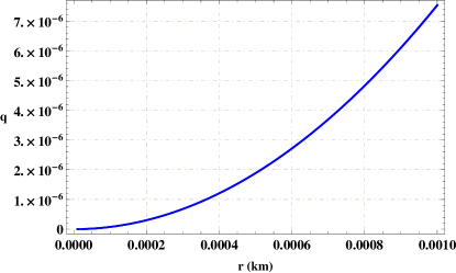
Figure 1: Graphical analysis of charge and thickness for $b=0.3$.

It is notable that the electric field is unaffected by the model parameter and has the same form as in GR. The charged shell’s thickness is incredibly thin and ranges between 0 and 1, i.e., $0<e^{-\lambda}\ll 1$. Moreover, the respective equations to this region are non-linear higher-order differential equations. Thus, obtaining an exact solution to the field equations is difficult. We have numerically solved the differential equation (31) by using the initial condition $\Phi(0)=0.1$ and obtained an interpolating function for the conformal factor corresponding to $b=0.3$ and $\beta=0.1$. The plot of charge against the thickness of shell has positive behavior as presented in Figure 1. Thus, the presence of charge provides an additional repulsive force that resists gravitational collapse leading to the formation of a more stable structure as compared to the uncharged model.

3.3 The Exterior Geometry and Israel Formalism

The Reissner-Nordström metric corresponds to this vacuum region obey the EoS $\varrho=\mathcal{P}=0$ and is expressed as follows

$$ds^{2}=\curlyvee(r)dt^{2}-\curlyvee(r)^{-1}dr^{2}-r^{2}(d\theta^{2}+\sin^{2}{\theta}d\phi^{2}),$$ (32)

where $\curlyvee(r)=1-\frac{2\mathcal{M}}{r}+\frac{\mathcal{Q}^{2}}{r^{2}}$, $\mathcal{M}$ is the total gravitational mass of gravastar and $\mathcal{Q}$ represents corresponding total charge. Its interesting to evaluate the constraints that will allow us to match the internal and external regions smoothly. In this context, Israel’s formalism plays key role in achieving the appropriate conditions of smooth matching. The metric coefficients must be continuous at the hypersurface $(\Sigma)$, i.e. at $r=\mathcal{R}$ but their derivatives might be discontinuous. We use Lanczos equations to determine the surface stress-energy tensor given as follows

$$S_{\beta}^{\alpha}=(\delta_{\beta}^{\alpha}\tau_{\gamma}^{\gamma}-\tau_{\beta}^{\alpha})\frac{1}{8\pi},$$ (33)

where $\tau_{\alpha\beta}=K^{+}_{\alpha\beta}-K^{-}_{\alpha\beta}$. It symbolizes the discontinuity in extrinsic curvature. The exterior and interior regions are characterized by positive and negative signs, respectively. Extrinsic curvature components at $(\Sigma)$ are represented as

$${K_{\alpha\beta}^{\pm}}=-n_{\zeta}^{\pm}\left[\frac{\partial^{2}x^{\zeta}}{\partial\xi^{\alpha}\xi^{\beta}}+\Gamma^{\zeta}_{\lambda\delta}\left(\frac{\partial x^{\lambda}}{\partial\xi^{\alpha}}\right)\left(\frac{\partial x^{\delta}}{\partial\xi^{\beta}}\right)\right],$$ (34)

where $\xi^{\beta}$ indicates the coordinates of intrinsic shell and $n_{\zeta}^{\pm}$ shows the unit normal at $\Sigma$. It is provided by

$$n_{\zeta}^{\pm}=\pm\left|g^{\lambda\delta}\frac{\partial\curlyvee}{\partial x^{\lambda}}\frac{\partial\curlyvee}{\partial x^{\delta}}\right|^{-\frac{1}{2}}\frac{\partial\curlyvee}{\partial x^{\zeta}},\quad n_{\zeta}n^{\zeta}=1.$$ (35)

For charged perfect fluid matter configuration, EMT takes the follwing form $S_{\beta}^{\alpha}=\text{diag}(\Psi,-\Omega,-\Omega)$, where $\Psi$ and $\Omega$ are surface energy density and surface pressure provided by Lanczos equations as

$$\Psi = -\frac{1}{4\pi\mathcal{R}}\left[\sqrt{\curlyvee}\right]_{-}^{+},$$ (36)

$$\Omega = -\frac{\varrho}{2}+\frac{1}{16\pi}\left[\frac{{\curlyvee^{{}^{\prime}}}}{\sqrt{\curlyvee}}\right]_{-}^{+}.$$ (37)

We obtain matter variables by inserting the metric functions of interior and exterior spacetimes in the preceding equations which leads to

$$\Psi = -\frac{1}{4\pi\mathcal{R}}\left[\sqrt{1-\frac{2\mathcal{M}}{\mathcal{R}}+\frac{\mathcal{Q}^{2}}{\mathcal{R}^{2}}}-\tilde{\Phi}_{0}\mathcal{R}\right],$$ (38)

$$\Omega = \frac{1}{8\pi\mathcal{R}}\left[\frac{\mathcal{R}-\mathcal{M}}{\mathcal{R}\sqrt{1-\frac{2\mathcal{M}}{\mathcal{R}}+\frac{\mathcal{Q}^{2}}{\mathcal{R}^{2}}}}-2\tilde{\Phi}_{0}\mathcal{R}\right].$$ (39)

Employing energy density at surface, the mass of the intrinsic shell is obtained as

$$\mathcal{M}_{shell}=4\pi\mathcal{R}^{2}\Psi=\left[\tilde{\Phi}_{0}\mathcal{R}-\sqrt{1-\frac{2\mathcal{M}}{\mathcal{R}}+\frac{\mathcal{Q}^{2}}{\mathcal{R}^{2}}}\right]\mathcal{R}.$$

As a result, the total mass of charged gravastar in terms of $\mathcal{M}_{shell}$ takes the form

$$\mathcal{M}=\frac{1}{2\mathcal{R}}\left[\mathcal{R}^{2}-\tilde{\Phi}_{0}^{2}\mathcal{R}^{6}-\mathcal{M}^{2}_{shell}{\mathcal{R}}^{2}+2\tilde{\Phi}_{0}\mathcal{M}_{shell}\mathcal{R}^{4}+\mathcal{Q}^{2}\right].$$ (40)

4 Some Physical Attributes of Charged Gravastars

The physical characteristics of charged gravastar, such as the EoS parameter, entropy, energy, and appropriate length, are discussed in this section.

4.1 The EoS Parameter

It describes the connection between matter variables, such as pressure and energy density of fluid configuration. Taking into account the effective variables of matter contents, we get the EoS parameter at $r=\mathcal{R}$ with following mathematical description $\omega(\mathcal{R})=\Omega/\Psi$. Substituting the corresponding values of matter variables, we obtain

$$\omega(\mathcal{R})=\frac{\Omega}{\Psi}=\frac{\frac{1}{8\pi\mathcal{R}}\left[\frac{\mathcal{R}-\mathcal{M}}{\mathcal{R}\sqrt{1-\frac{2\mathcal{M}}{\mathcal{R}}+\frac{\mathcal{Q}^{2}}{\mathcal{R}^{2}}}}-2\tilde{\Phi}_{0}\mathcal{R}\right]}{-\frac{1}{4\pi\mathcal{R}}\left[\sqrt{1-\frac{2\mathcal{M}}{\mathcal{R}}+\frac{\mathcal{Q}^{2}}{\mathcal{R}^{2}}}-\tilde{\Phi}_{0}\mathcal{R}\right]}.$$ (41)

This equation includes different fractional components as well as square root terms that makes the equation more complex. To attain real EoS parameter, the basic requirement is either $\frac{2\mathcal{M}}{\mathcal{R}}-\frac{\mathcal{Q}^{2}}{\mathcal{R}^{2}}<1$, or $\frac{2\mathcal{M}}{\mathcal{R}}<1$. The obtained relation among $\mathcal{M}$, $\mathcal{R}$ and $\mathcal{Q}$ is $\mathcal{Q}>\sqrt{\mathcal{R}(2\mathcal{M}-\mathcal{R})}$ and $\mathcal{M}<\frac{\mathcal{R}}{2}$. It is observed that positive pressure and energy density correspond to a positive value of the EoS parameter and $\omega(\mathcal{R})\approx 1$ is acquired for higher values of $\mathcal{R}$ [50]. These values of $\mathcal{R}$ illustrate the perspective of cold compact objects like gravastars and the absence of pressure makes it equivalent to a dust shell.

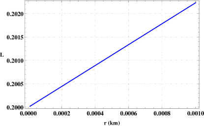
Figure 2: Graphical trend of the proper length and thickness for $b=0.3$ and $\beta=0.1$.

4.2 Proper Length

The proper length of charged gravastar is measured from interior region boundary $r_{1}=\mathcal{R}$ to the thin-shell boundary $r_{2}=\mathcal{R}+\epsilon$, where $\epsilon$ is incredibly small thickness of charged shell. Consequently, we have

$${L}=\int_{\mathcal{R}}^{\mathcal{R}+\epsilon}\sqrt{e^{\lambda}}dr.$$ (42)

Differentiation of Eq.(42) provides

$$L^{\prime}(r)=\frac{b}{\Phi}\Big{|}_{\mathcal{R}}^{\mathcal{R}+\epsilon}.$$ (43)

In order to graphically analyze the behavior of length, we use the numerical solution of $\Phi$ and solve Eq.(43) for the initial condition $L(0)=0.2$. The length of the charged thin-shell shows an increasing profile against the thickness of the shell as shown in Figure 2.

4.3 Entropy of Shell

Within the core of charged gravastar, entropy is a measure of randomness or disorderness in the respective region. The entropy density of the interior region is found to be zero in the literature [13]. Inside the charged shell, the entropy is given by [52]

$$S=4\pi\int_{\mathcal{R}}^{\mathcal{R}+\epsilon}\sqrt{e^{\lambda}}r^{2}\verb"s"(r)dr,$$ (44)

where entropy density is denoted by $\verb"s"(r)$ and its mathematical description is as follows

$$\verb"s"(r)=\frac{\Upsilon^{2}w_{\beta}^{2}{T}(r)}{4\pi{\hslash^{2}}}=\Upsilon\left(\frac{w_{\beta}}{\hslash}\right)\sqrt{\frac{\mathcal{P}}{2\pi}},$$ (45)

where $\Upsilon$ is a scalar constant, $T(r)$ is the temperature, $\hslash$ is Planck’s constant and $w_{\beta}$ is Boltzmann constant. As changing the value of a constant simply scales the graph, therefore the physical trend of the variables is not affected. For convenience, we take $\hslash=w_{\beta}=1$. Consequently, entropy turns out to be

$$S=\int_{\mathcal{R}}^{\mathcal{R}+\epsilon}\frac{4\pi\Upsilon r^{2}}{\sqrt{2\pi}}\sqrt{\mathcal{P}e^{\lambda}}dr.$$ (46)

Substitution Eq.(29) and $e^{\lambda}=(\frac{b}{\Phi})^{2}$ leads to the following form

$$S=\int_{\mathcal{R}}^{\mathcal{R}+\epsilon}\frac{b\sqrt{8\pi}\Upsilon}{\Phi}\Bigg{[}\frac{{\sqrt{b^{2}r^{2}(b^{2}(\Xi)-8\beta r\Phi\Phi^{\prime}-16\beta\Phi^{2})}}}{4b^{2}\beta r^{2}}+\frac{1}{4\beta}\Bigg{]}^{\frac{1}{2}}r^{2}dr,\\$$ (47)

whose differentiation provides

$$S^{\prime}(r)=\frac{b\sqrt{8\pi}\Upsilon}{\Phi}\Bigg{[}\frac{\sqrt{b^{2}r^{2}(b^{2}(\Xi)-8\beta r\Phi\Phi^{\prime}-16\beta\Phi^{2})}}{4b^{2}\beta r^{2}}+\frac{1}{4\beta}\Bigg{]}^{\frac{1}{2}}r^{2}\Big{|}_{\mathcal{R}}^{\mathcal{R}+\epsilon}.\\$$ (48)

The interpolating function of entropy is obtained by numerically solving Eq.(48) along with the initial condition $S(0)=0.2$. The plot shows that the entropy of shell increases. Thus, charge and the correction terms of $f(\mathfrak{R},\mathbf{T}^{2})$ gravity play a key role in increasing the randomness of the geometrical structure (refer to Figure 3).

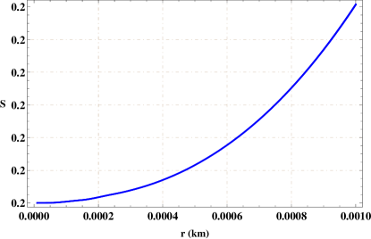
Figure 3: Behavior of shell’s entropy versus thickness of the shell for $b=0.3$ and $\beta=0.1$.

4.4 Shell Energy

The charged gravastar’s inner region has repulsive behavior and meets the following EoS $\varrho=-\mathcal{P}$. In charged gravastar, this repulsive character avoids singularity formation, while the energy contained within thin-shell is illustrated as [51]

$$\mathcal{E}=\frac{1}{2}\int_{\mathcal{R}}^{\mathcal{R}+\epsilon}\left(\varrho+2\pi{E}^{2}\right)r^{2}dr,$$ (49)

which simplifies to

$$\mathcal{E} = \int_{\mathcal{R}}^{\mathcal{R}+\epsilon}\left(\frac{\sqrt{b^{2}r^{6}\left(b^{2}\left(20\beta+r^{2}\right)-120\beta r\Phi\Phi^{\prime}\right)}}{40b^{2}\beta r^{2}}-\frac{r^{2}}{40\beta}\right.$$ (50)

$$+ \left.\frac{40r\Phi\Phi^{\prime}}{40b^{2}}-\frac{40\Phi^{2}}{40b^{2}}+\frac{1}{2}\right)dr.$$

Differentiation of the above equation leads to

$$\mathcal{E}^{\prime}(r)=\frac{\sqrt{b^{2}r^{6}\left(b^{2}\left(20\beta+r^{2}\right)-120\beta r\Phi\Phi^{\prime}\right)}}{40b^{2}\beta r^{2}}-\frac{r^{2}}{40\beta}+\frac{r\Phi\Phi^{\prime}}{b^{2}}-\frac{\Phi^{2}}{b^{2}}+\frac{1}{2}\Big{|}_{\mathcal{R}}^{\mathcal{R}+\epsilon}.$$ (51)

The numerical solution of above equation is obtained by using initial condition $\epsilon(0)=0.2$ which is plotted in Figure 4. It describes the increasing trend of the intrinsic shell energy against $\epsilon$.

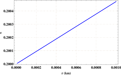
Figure 4: Graphical trend of shell’s energy and thickness for $b=0.3$ and $\beta=0.1$.

5 Final Remarks

In this paper, we have investigated the influence of charge on an alternate model of a black hole, dubbed as gravastar in EMSG. For this purpose, we have considered a setup admitting conformal motion corresponding to a minimally coupled linear model, i.e., $f(\mathfrak{R},\textbf{T}^{2})$=$\mathfrak{R}+\beta\textbf{T}^{2}$. We have adopted a linear EoS $\varrho=\omega\mathcal{P}$ to inspect different regions of charged gravastar. For the interior dS spacetime, we take $\omega=-1$ to incorporate negative pressure which maintains the balance of forces and avoids the formation of a singularity. The shell of small thickness corresponds to the intermediate region filled with baryonic matter and obeying $\omega=1$. We have represented the vacuum exterior of the charged gravastar through Reissner-Nordström black hole satisfying $\varrho=\mathcal{P}=0$. Israel junction conditions have provided surface density and pressure which help to determine the mass of charged thin-shell as well as the total gravitational mass. We have graphically inspected the role of electromagnetic field for different values of $\beta$. In the current scenario, physically viable and stable geometry of gravastar is obtained for $\frac{2\mathcal{M}}{\mathcal{R}}-\frac{\mathcal{Q}^{2}}{\mathcal{R}^{2}}<1$. Figures 2-4 demonstrate that the proper length, entropy and energy increases against the thickness of the shell in the presence of charge.

We have found that the length, entropy and energy of the gravastar structure increase in the presence of charge. Also, in other modified theories of gravity, the graphical analysis of various features has shown that the physical attributes of the shell follow an increasing trend [53]-[55]. Thus, our analysis provides consistent results with other modified theories of gravity. Moreover, as the charge provides a positive outward-directed force, therefore, an additional repulsive force helps the gravastar from collapsing into a singularity. Thus, the presence of charge generates a more stable structure as compared to the uncharged model. Our analysis follows the consistent increasing trend of length, energy and entropy of charged analogs presented in GR as well as other modified theories of gravity [36, 37, 39, 40]. Furthermore, we have found that under the influence of ${f}(\mathfrak{R},\textbf{T}^{2})$ gravity, the physical attributes of gravastar have greater values of length, energy and entropy in comparison to work presented in GR and ${f(\mathfrak{R},T)}$ gravity [36, 37]. Recently, Sharif and Saeed [43] studied charge-free gravastar accepting conformal motion in background of $f(\mathfrak{R},\textbf{T}^{2})$ gravity and concluded that proper length decreases while entropy as well as energy increases abruptly. In contrast to the uncharged case, in the presence of charge proper length, energy and entropy increase with respect to thickness of the shell. We conclude that $f(\mathfrak{R},\textbf{T}^{2})$ gravity satisfactorily discusses charged gravastar model admitting conformal motion and provides more stable structure in comparison to uncharged analog [43]. It is noteworthy that our results reduce to GR for $\beta=0$ [34].

Data availability: No new data were generated or analyzed in support of this research.

References

- [1] Pietrobon, D., Balbi, A. and Marinucci, D.: Phys. Rev. D 74(2006)043524; Astieer, P. et al.: Astron. Astrophys 447(2016)31.
- [2] Felice, A.D. and Tsujikawa, S.R.: Living Rev. Relativ. 13(2010)3; Nojiri, S. and Odintsov, S.D.: Phys. Rep. 505(2011)59; Bamba, K. et al.: Astrophys. Space Sci. 342(2012)155.
- [3] Harko, T., Koivisto, T.S. and Lobo, F.S.N.: Mod. Phys. Lett. A 26(2011)1467.
- [4] Haghani, Z. et al.: Phys. Rev. D 88(2013)044023.
- [5] Katirci, N. and Kavuk, M.: Eur. Phys. J. Plus. 129(2014)163.
- [6] Roshan, M. and Shojai, F.: Phys. Rev. D 94(2016)044002.
- [7] Board, C.V.R. and Barrow, J.D.: Phys. Rev. D 96(2017)123517.
- [8] Nari, N. and Roshan, M.: Phys. Rev. D 98(2018)024031.
- [9] Akarsu, O. et al.: Phys. Rev. D 98(2018)063522.
- [10] Moraes, P.H.R.S. and Sahoo, P.K.: Phys. Rev. D 97(2018)024007.
- [11] Bahamonde, S., Marciu, M. and Rudra, P.: Phys. Rev. D 100(2019)083511.
- [12] Sharif, M. and Gul, M.Z.: Phys. Scr. 96(2020)025002; Int. J. Mod. Phys. A 36(2021)2150004; Adv. Astron. 2021(2021)6663502; Eur. Phys. J. Plus 136(2021)503; Chin. J. Phys. 71(2021)365; Universe 07(2021)154; Phys. Scr. 96(2021)105001.
- [13] Mazur, P. and Mottola, E.: Proc. Natl. Acad. Sci. 101(2004)9545.
- [14] Sakai, N. et al.: Phys. Rev. D 90(2014)104013.
- [15] Kubo, T. and Sakai, N.: Phys. Rev. D 93(2016)084051.
- [16] Cardoso, V. et al.: Phys. Rev. Lett. 116(2016)171101.
- [17] Cardoso, V. et al.: Phys. Rev. Lett. 117(2016)089902.
- [18] Akiyama, K. et al.: Astrophys. J. Lett. 875(2019)1.
- [19] Visser, M. and Wiltshire, D.L.: Class. Quantum Grav. 21(2004)1135.
- [20] Carter, B.M.N.: Class. Quantum Grav. 22(2005)4551.
- [21] Cattoen, C., Faber, T. and Visser, M.: Class. Quantum Grav. 22(2005)4189.
- [22] Bilic, N., Tupper, G.B. and Viollier, R.D.: J. Cosmol. Astropart. Phys. 02(2006)013.
- [23] Hovart, D. and Ilijic, S.: Class. Quantum Grav. 24(2007)5637.
- [24] Ghosh, S. et al.: Phys. Lett. B 767(2017)380.
- [25] Debnath, U.: Eur. Phys. J. C 79(2019)499.
- [26] Bhatti, M.Z. et al.: Phys. Dark Universe 29(2020)100561; Das, A., et al.: Nucl. Phys. B 954(2020)114986; Yousaf, Z.: Phys. Dark Universe 28(2020)100509; Shamir, M.F. and Zia, S.: Can. J. Phys. 98(2020)9.
- [27] Sharif, M. and Waseem, A.: Eur. Phys. J. Plus. 135(2020)930.
- [28] Abbas, G. and Majeed, K.: Adv. Astron. 2020(2020)8861168.
- [29] Herrera, L. and Leon, J.P.D.: J. Math. Phys. 26(1985)2302.
- [30] Banerjee, A. et al.: Eur. Phys. J. C 76(2016)34.
- [31] Lobo, F.S.N. and Arellano, A.V.B.: Class. Quantum Grav. 24(2007)1069.
- [32] Horvat, D., Ilijic, S. and Marunovic, A.: Class. Quantum Grav. 26(2009)025003.
- [33] Turimov, B.V., Ahmedov, B.J. and Abdujabbarov, A.A.: Mod. Phys. Lett. A 24(2009)733.
- [34] Usmani, A.A. et al.: Phys. Lett. B 701(2011)388.
- [35] Rahaman, F. et al.: Phys. Lett. B 717(2012)1.
- [36] Sharif, M. and Javed, F.: Ann. Phys. 415(2020)168124; J. Exp. Theor. Phys. 132(2021)381; Eur. Phys. J. C 81(2021)47.
- [37] Sharif, M. and Waseem, A.: Astrophys. Space Sci. 364(2019)189.
- [38] Bhatti, M.Z. et al.: Phys. Dark Universe 29(2020)100561.
- [39] Bhar, P. and Rej, P.: Eur. Phys. J. C. 81(2021)763.
- [40] Bhatti, M.Z. et al.: Chin.J.Phys. 73(2021)167; Mod. Phys. Lett. 36(2021)2150233.
- [41] Azmat, H. Zubair, M. and Ahmad, Z. Ann. Phys. 439(2022)168769.
- [42] Sharif, M., and Naz, S. Universe 8(2022)142.
- [43] Sharif, M. and Saeed, M.: Chin. J. Phys. (to appear, 2022).
- [44] Faraoni, V.: Phys. Rev. D 80(2009)124040.
- [45] Akarsu, O. et al.: Phys. Rev. D 97(2018)024011.
- [46] Zeldovich, Y.B.: Mon. Not. R. Astron. Soc. 160(1972)1.
- [47] Carr, B.J.: Astrophys. J. 201(1975)1.
- [48] Wesson, P.S.: J. Math. Phys. 19(1978)2283.
- [49] Madsen, M.S. et al.: Phys. Rev. D 46(1992)1399.
- [50] Rahaman, F. et al.: Phys. Lett. B 707(2012)319.
- [51] Wesson, P.S.: Vistas Astron. 29(1986)281; Braje, T.M. and Romani, R.W.: Astrophys. J. 580(2002)1043; Linares, L.P., Malheiro, M. and Ray, S.: Int. J. Mod. Phys. D 13(2004)1355.
- [52] Ghosh, S. et al.: Phys. Lett. B 380(2017)767.
- [53] Das, A. et al.: Phys. Rev. D 95(2017)124011.
- [54] Shamir, F. and Ahmad, M.: Phys. Rev. D 97(2018)104031.
- [55] Yousaf, Z., Bhatti, M.Z. and Asad, H.: Phys. Dark Universe 28(2020)100527.