On the free rotation of a polarized spinning-top as a test of the correct radiation reaction torque.

Abstract

The formula for dipole radiation reaction torque acting on a system of charges, and the Larmor-like formula for the angular momentum loss by this system, differ in the time derivative term which is the analogue of the Schott term in the energy loss problem. In the well-known textbooks this discrepancy is commonly avoided via neglect of the Schott term, and the Larmor-like formula is preferred. In the present paper both formulae are used to derive two different equations of motion of a polarized spinning-top. Both equations are integrable for the symmetric top and lead to quite different solutions. That one following from the Larmor-like formula is physically unplausible, in contrast to another one. This result is accorded with the reinterpretation of Larmor’s formula discussed recently in the pedagogical literature. It is appeared, besides, that the Schott term is of not only academic significance, but it may determine the behavior of polarized micro- and nanoparticles in nature or future experiments.

Video-abstract:
https://www.dropbox.com/s/im6tmkdrr3oh3ud/EJP_ac578c_Video_Abstr.mov?dl=0

Keywords: radiation reaction, Schott term, spinning-top

1 Introduction

It is known that an intensity of the radiation emitted by a system of charged particles, as it follows from the Larmor formula, contradicts to the power of the radiation reaction force acting on the particles, and the difference of these quantities is dependent of a jerk and is a rate of the change of so called Schott energy [2, 3].

The notion of acceleration-dependent Schott energy is known for a long time, and recently it has attracted attention as a subject of graduate electrodynamics courses [3, 4, 5, 6]. The physical interpretation of this notion is still debatable as referring to ill-defined concepts, such as the point-like charge, electromagnetic mass etc [4, 7].

Another question is how significant is the Schott term in the energy balance equation of the system of moving charges. This is a question of correct application of the Larmor formula and related equations in practice, in particular, in teaching tasks for students.

In many classic textbooks on electrodynamics, such as by Jackson [8, Sect. 16.2], by Panofsky & Phillips [9, Sect. 21-6], or by Griffiths [10, Sect. 11.2.2], the Larmor formula is used to derive the equation of motion of charged particles taking into account the radiation reaction. One requires, upon derivations, a zero contribution of the Schott term, at least on average over a time of interest (in particular, over a period in a periodic motion).

Sometimes there is regarded obvious (as in the Landau & Lifshitz textbook [11, § 75]), that the Schott term is negligibly small if limited to a nearly stationary motion of a system of charges. Therefore, it may seem that the Larmor formula or its relativistic generalization, the Liénard formula, are sufficient for accounting the effect of radiation reaction on the motion of charges.

In fact, this is not the case since the value and the role of the Schott term may be different. This follows from several examples of the relativistic mechanics of charged particles presented in literature. For one, in a periodic particle motion, not only an averaged value [6] but also the instant value [13] of the Schott term may occur small. On the other hand, the Liénard formula (where the Schott term is absent) leads to a finite error in pitch of trajectory when considering a motion of charged particle in a magnetic field [14]. Upon uniformly accelerated motion, the Schott term is increasingly negative [5] while the radiation reaction in zero. Thus a care must be taken when handling with the Schott term and Larmor formula.

Fortunately, there are known the equations of motion (and the above examples are based on them) derived via several ways regardless of the Larmor formula or energy balance condition [2, 11, 15, 16, 17]. These are the Lorentz-Abraham-Dirac equation [18] or its nonrelativistic predecessor known as the Abraham-Lorentz equation [19] which both are widely accepted.

In turn, it is possible from these equations to deduce unambiguously the energy balance equation [11, § 75] containing the Schott term, whatever its magnitude.

Similarly to the intensity of radiation, but less often, there is considered in textbooks the flux of angular momentum which being lost by charges via radiation.

For a single particle in a conservative central field the loss rate of the angular momentum is given in the textbook [8]; for a system of charges the corresponding formula was derived in [11, § 72,§ 75].

As in the case of energy, this formula does not agree with the torque of radiation reaction forces against charges, and the difference is equal to the rate of change of a vector quantity referred here to as the Schott angular momentum. The aforementioned textbooks suggest, by analogy with the case of energy, to neglect the corresponding Schott term in the balance equation of angular momentum as well.

It is demonstrated in the present work that, in general, this suggestion is not correct and may lead to a mistaken picture of behavior of even nonrelativistic systems. For this purpose we consider a free spinning-top possessing a constant proper electric dipole moment.

The translational motion of such a spinning-top is described by a physical solution of the Abraham-Lorentz equation for a free particle, i.e., the trivial motion by inertia. In order to include the rotational degrees of freedom, the Abraham-Lorentz equation is not sufficient: one have apply the balance equation of angular momentum. The question arises: should a Schott term be included in this equation? In both cases (with and without this term) the balance equation can be reduced to nonlinear equations of the Euler type which are integrable provided the spinning-top is axially symmetric. These equations involve higher-order kinematics and themselves are of pedagogical interest as new solvable examples of rigid body dynamics. The solutions found in both cases differ essentially from each other, and represent completely different evolutions of the spinning-top. Thus, there is a question of choosing correct angular momentum balance equation, which is discussed in final section.

The considered problem is not purely academic. Nowadays, nanoparticles in optical traps can be spun up to GHz [20, 21]. On the other hand, the dipole moment of some artificially created nanocrystals reaches hundreds and thousands Debyes [22, 23] (and moreover expected up to 10${}^{7}\,$ D [24]). Under such trends, the effects of radiative spindown may soon become observable experimentally [25], and their theoretical description should be relevant.

2 Angular momentum balance equation for a system of charges.

Let us consider a nonrelativistic system of charges $q$ with masses $m$ situated in positions $\boldsymbol{r}(t)$ and moving with velocities $\dot{\boldsymbol{r}}\equiv{\rm d}{\boldsymbol{r}}\,/{\rm d}{t}\,$ much smaller than speed of light $c$. Such a system loses an energy via the dipole radiation (other multipole components are negligibly small in the nonrelativistic approximation). Similarly, the system loses an angular momentum, and this loss can be taken into account variously. The Landau & Lifshitz textbook suggests two methods.

The 1st method, similar to deriving the Larmor formula, consists in accounting the flux of the angular momentum of the dipole radiation through the sphere embracing the charges, and leads to the following formula (see [11], §72, Problem 2, equation (3); also equation (75.7))

$$\frac{{\rm d}{\boldsymbol{L}}\,}{{\rm d}{t}\,}=-\frac{2}{3c^{3}}\,\dot{\boldsymbol{\mathfrak{d}}}\times\ddot{\boldsymbol{\mathfrak{d}}}$$ (2.1)

for the angular momentum $\boldsymbol{L}=\sum m\,\boldsymbol{r}\times\boldsymbol{v}$, where $\boldsymbol{\mathfrak{d}}=\sum q\boldsymbol{r}$ is a dipole moment of a system; here the summation runs over all particles of the system. The 2nd method is based on calculating the torque of the Abraham-Lorentz forces of a radiation reaction; it yields another formula (look for unnumbered equation in [11, § 75]):

$$\frac{{\rm d}{\boldsymbol{L}}\,}{{\rm d}{t}\,}=\frac{2}{3c^{3}}\,\boldsymbol{\mathfrak{d}}\times\dddot{\boldsymbol{\mathfrak{d}}}.$$ (2.2)

To agree with the formula (2.1), the authors of [11] represented the expression on the right-hand side (r.-h.s.) of (2.2) as follows:

$$\boldsymbol{\mathfrak{d}}\times\dddot{\boldsymbol{\mathfrak{d}}}=\frac{{\rm d}{}\,}{{\rm d}{t}\,}\boldsymbol{\mathfrak{d}}\times\ddot{\boldsymbol{\mathfrak{d}}}-\dot{\boldsymbol{\mathfrak{d}}}\times\ddot{\boldsymbol{\mathfrak{d}}},$$ (2.3)

and then claimed that total time derivative (the 1st term in r.-h.s.) vanish upon averaging over a stationary motion (implying a nearly stationary motion; see footnote${}^{\ref{Rem1}}$ on page 2). The result is the formula (2.1).

It is convenient, by analogy to the notion of Schott energy, to introduce the vector quantity referred here to as the Schott angular momentum:

$$\boldsymbol{L}_{\rm S}\equiv\frac{2}{3c^{3}}\boldsymbol{\mathfrak{d}}\times\ddot{\boldsymbol{\mathfrak{d}}}=\frac{2}{3c^{3}}\frac{{\rm d}{}\,}{{\rm d}{t}\,}\boldsymbol{\mathfrak{d}}\times\dot{\boldsymbol{\mathfrak{d}}}.$$ (2.4)

Then the r.-h.s. of (2.2) can be reduced, by accounting (2.3), to the r.-h.s. of (2.1) plus the Schott term $\dot{\boldsymbol{L}}_{\rm S}$ (i.e., the rate of change of the Schott angular momentum) which is considered in [11, § 75] negligibly small.

In Jackson textbook [8, Sect. 16.2] the Abraham-Lorentz equation for a particle in the external central field $V(r)$,

$$m\dot{\boldsymbol{v}}=\boldsymbol{F}_{\!\!\rm ex}+\frac{2q^{2}}{3c^{3}}\ddot{\boldsymbol{v}},\qquad\mbox{where}\quad\boldsymbol{F}_{\!\!\rm ex}=-\frac{{\rm d}{V}\,}{{\rm d}{r}\,}\frac{\boldsymbol{r}}{r},$$ (2.5)

is used to derive the balance equation of the particle angular momentum $\boldsymbol{L}=m\boldsymbol{r}\times{\boldsymbol{v}}$:

$$\frac{{\rm d}{\boldsymbol{L}}\,}{{\rm d}{t}\,}=\frac{2q^{2}}{3c^{3}}\boldsymbol{r}\times\ddot{\boldsymbol{v}}.$$ (2.6)

Here is used the fact that the torque of an external central force vanish, $\boldsymbol{r}\times\boldsymbol{F}_{\!\!\rm ex}=0$. The remaining term in r.-h.s. can again be presented as follows:

$$\frac{2q^{2}}{3c^{3}}\boldsymbol{r}\times\ddot{\boldsymbol{v}}=\tau_{0}\frac{{\rm d}^{2}{\boldsymbol{L}}\,}{{\rm d}{t^{2}}\,}-\frac{2q^{2}}{3c^{3}}\boldsymbol{v}\times\dot{\boldsymbol{v}},$$ (2.7)

where $\tau_{0}=2q^{2}/(3mc^{3})$ is a small parameter of the dimension of time (for the electron we have $\tau_{0}\approx(2/3){\times}10^{-23}$s.). One supposes in [8, Sect. 16.2] that the angular momentum $\boldsymbol{L}$ little changes during the time $\tau_{0}$. Thus the 1st term (i.e., the Schott term) $\dot{\boldsymbol{L}}_{\rm S}=\tau_{0}\ddot{\boldsymbol{L}}$ can be neglected, and the equation (2.6) reduces to the form:

$$\frac{{\rm d}{\boldsymbol{L}}\,}{{\rm d}{t}\,}=-\frac{2q^{2}}{3c^{3}}\boldsymbol{v}\times\dot{\boldsymbol{v}}.$$ (2.8)

Then, the acceleration in the 2nd term of r.-h.s. is to be expressed via the external force by an unperturbed equation of motion . Finally, one obtains the balance equation:

$$\frac{{\rm d}{\boldsymbol{L}}\,}{{\rm d}{t}\,}=-\frac{\tau_{0}}{m}\left\langle\frac{1}{r}\frac{{\rm d}{V}\,}{{\rm d}{t}\,}\right\rangle\boldsymbol{L},$$ (2.9)

in which the averaging $\langle\dots\rangle$ is performed over a particle orbit. It follows from this equation that $|\dot{\boldsymbol{L}}|=O(\tau_{0})$, then $|\dot{\boldsymbol{L}}_{\rm S}|=|\tau_{0}\ddot{\boldsymbol{L}}|=O(\tau_{0}^{3})$, which is negligibly small as compared to r.-h.s. of (2.9). Thus the Schott term was neglected reasonably.

Before giving a counterexample in which the neglect of the Schott term is erroneous, the following caveat should be made.

The equations presented in this section reveal the inconsistency that they are based on the Newtonian (i.e., nonrelativistic) dynamics, supplemented by the dipole radiation correction. The latter arises from the relativistic theory as a term of order $1/c^{3}$ in the $1/c$ expansion of the Liènard-Wiechert potentials. Other multipole contributions have orders of magnitude $1/c^{5}$ and higher, and are negligibly small for slow-moving charges.

Along with dipole radiation terms, the dynamics should take into account post-Newtonian corrections of the order of $1/c^{2}$, which arise from relativistic kinematics and potentials of interparticle interaction [11, § 65]. However, for a conservative system (such as a closed system of charges or a particle in the central field), post-Newtonian corrections are also conservative, and lead to effects other than the dissipative radiative damping. For example, in the classical hydrogen atom problem, the post-Newtonian terms does not destroy the periodicity of motion, but only cause a perihelion advance, while the radiation reaction leads to a fall to the center. (In the quantum problem, the $c^{-2}$–corrections split the spectral lines, while $c^{-3}$ broad them). The nonrelativistic approximation is used in other cases, for example, when taking into account the radiation effects in the Penning trap [27, Sect. 7.4]; the post-Newtonian effects are analyzed separately [27, Sect. 7.6]; see also [28].

The next sections will study the effect of radial reaction on the rotational motion of a composite particle considered as a nonrelativistic rigid body with a proper dipole moment. From a practical viewpoint, such a consideration is appropriate, since in the mentioned in the Introduction examples [20, 21] of a 100 nm particle spined up to GHz, the velocity of its components does not exceed 10${}^{-6}c$. At this point, however, the principal inconsistency arises as the notion of rigid body contradicts to the relativity [29, Sect. 45]. Instead, one should consider a (confined) deformed elastic medium which, in the post-Newtonian approximation, can be close to the rigid one, the so called quasirigid body [30]. Mechanical properties of this body are determined by the energy-momentum tensor of the medium, and can be defined in such a way that, in the post-Newtonian approximation, they entirely are expressed via corrections to the inertia tensor.

Therefore, at least within this model, $c^{-3}$ radiation effects can be combined directly with the nonrelativistic rigid body dynamics. This consideration will be used in subsequent sections.

In general case of quasirigid body, the post-Newtonian $c^{-2}$ corrections to the dynamics are more complicated but still conservative, and their neglect should not misrepresent the dissipative radiation effects.

3 Equations of motion of free polarized spinning-top

Let a system of charges be a composite particle considered as a rigid body, i.e., a spinning-top. If the spinning-top is free, then its translational motion is a trivial motion by inertia. A rotational motion of the spinning-top can be described by means of the angular momentum balance equation. Let us represent for this purpose an arbitrary point $\boldsymbol{r}(t)$ of the top as follows: $\boldsymbol{r}(t)=\mathsf{O}(t)\boldsymbol{\rho}$, where $\mathsf{O}(t)\in\$SO(3) is a rotation matrix, and $\boldsymbol{\rho}$ is constant (in time) position of this point in the proper reference frame of the top. Hence the relations follow:

$$\boldsymbol{v} \equiv \dot{\boldsymbol{r}}=\dot{\mathsf{O}}\boldsymbol{\rho}=\mathsf{O}(\boldsymbol{\Omega}\times\boldsymbol{\rho}),$$

$$\dot{\boldsymbol{v}} = \mathsf{O}\{\boldsymbol{\Omega}\times(\boldsymbol{\Omega}\times\boldsymbol{\rho})+\dot{\boldsymbol{\Omega}}\times\boldsymbol{\rho}\},$$ (3.1)

where $\boldsymbol{\Omega}$ is the angular velocity vector of the spinning-top in its proper reference frame which is dual to the skew-symmetric matrix $\mathsf{\Omega}\equiv\mathsf{O}^{\rm T}\dot{\mathsf{O}}$. In general, an arbitrary vector $\boldsymbol{\alpha}$ in the proper reference frame and its image $\boldsymbol{a}=\mathsf{O}\boldsymbol{\alpha}$ in the laboratory reference frame are related as follows:

$$\dot{\boldsymbol{a}}=\mathsf{O}\{\dot{\boldsymbol{\alpha}}+\boldsymbol{\Omega}\times\boldsymbol{\alpha}\}.$$ (3.2)

These kinematic relations can be used in the angular momentum balance equation in order to derive the Euler type equation of a rotational motion.

At this point the the dilemma arises – which balance equation to choose: (2.1) or (2.2) ? Let us consider both possibilities.

Substituting the relations (3) into (2.1) yields the equation:

$$\mathsf{I}\dot{\boldsymbol{\Omega}}+\boldsymbol{\Omega}\times\mathsf{I}\boldsymbol{\Omega} = -\frac{2}{3c^{3}}\{(\boldsymbol{d}\times\boldsymbol{\Omega})^{2}\boldsymbol{\Omega}+(\boldsymbol{d}\cdot(\boldsymbol{\Omega}\times\dot{\boldsymbol{\Omega}}))\boldsymbol{d}\},$$ (3.3)

where $\mathsf{I}=||I_{ij}||$ ($i,j=1,2,3$) is the inertia tensor, and $\boldsymbol{d}\equiv\mathsf{O}^{\rm T}\boldsymbol{\mathfrak{d}}=\sum m\boldsymbol{\rho}$ is a constant dipole moment of the spinning-top in its proper reference frame.

Similarly, the usage of (3) and (3.2) in (2.2) leads to the equation:

$$\mathsf{I}\dot{\boldsymbol{\Omega}}+\boldsymbol{\Omega}\times\mathsf{I}\boldsymbol{\Omega} = \frac{2}{3c^{3}}\boldsymbol{d}\times\{\boldsymbol{d}\times(\Omega^{2}\boldsymbol{\Omega}-\ddot{\boldsymbol{\Omega}})$$ (3.4)

$$\hskip 43.05542pt{}+(\boldsymbol{d}\cdot\dot{\boldsymbol{\Omega}})\boldsymbol{\Omega}+2(\boldsymbol{d}\cdot\boldsymbol{\Omega})\dot{\boldsymbol{\Omega}}\};$$

where $\Omega\equiv|\boldsymbol{\Omega}|$. This equation is a counterpart of the Abraham-Lorentz equation for the spinning-top, and it will be referred here to as the Abraham-Lorentz-Euler (ALE) equation. The equation (3.3) with the Schott term neglected (as compared to (3.4)) will be called as the truncated ALE equation.

In order to have a complete description of the spinning-top dynamics in space we complement the Euler type equations (3.3) or (3.4) by the Poisson equations:

$$\Omega_{1} = \dot{\varphi}\sin\theta\sin\psi+\dot{\theta}\cos\psi,$$

$$\Omega_{2} = \dot{\varphi}\sin\theta\cos\psi-\dot{\theta}\sin\psi,$$

$$\Omega_{3} = \dot{\varphi}\cos\theta+\dot{\psi},$$ (3.5)

relating the components of the angular velocity $\boldsymbol{\Omega}=\{\Omega_{1},\Omega_{2},\Omega_{3}\}$ with the Euler angles $\varphi,\theta,\psi$.

4 The dynamics of axially-symmetric spinning-top

4.1 Truncated Abraham-Lorentz-Euler equations

Henceforth the specific case will be considered of the axially-symmetric spinning-top with a dipole moment directed along the symmetry axis:

$$I_{ij}=I_{i}\delta_{ij}\quad(i,j=1,2,3),\quad I_{2}=I_{1};\qquad d_{1}=d_{2}=0,\quad d_{3}\equiv d$$ (4.1)

(there is no summation over $i$). Besides, we assume $I_{1}\neq 0$, $I_{3}\neq 0$. Then the equation (3.3) splits into the following nonlinear set:

$$\dot{\Omega}_{1}-(1-I_{3}/I_{1})\Omega_{2}\Omega_{3}=-\tau\Omega_{\bot}^{2}\Omega_{1},$$ (4.2)

$$\dot{\Omega}_{2}+(1-I_{3}/I_{1})\Omega_{1}\Omega_{3}=-\tau\Omega_{\bot}^{2}\Omega_{2},$$ (4.3)

$$\dot{\Omega}_{3}=-\tau\Omega_{\bot}^{2}\Omega_{3};$$ (4.4)

here $\Omega_{\bot}=|\boldsymbol{\Omega}_{\bot}|=\sqrt{\Omega_{1}^{2}+\Omega_{2}^{2}}$, where $\boldsymbol{\Omega}_{\bot}=\{\Omega_{1},\Omega_{2},0\}$, and again the small parameter of the dimension of time is introduced: $\tau=2d^{2}/(3I_{1}c^{3})$.

In order to solve this set of differential equations let us first multiply (4.2) by $\Omega_{2}$, (4.3) by $\Omega_{1}$, and add them yielding the equation for $\Omega_{\bot}$:

$$\dot{\Omega}_{\bot}=-\tau\Omega_{\bot}^{3}.$$ (4.5)

The solution of this equation, $\Omega_{\bot}(t)=\Omega_{\bot 0}/R(t)$, where

$$R(t)\equiv\sqrt{1+2\tau\Omega_{\bot 0}^{2}t},\quad\Omega_{\bot 0}\equiv\Omega_{\bot}(0),$$ (4.6)

is to be substituted into (4.4), and then into (4.2), (4.3) reducing a whole set of equations to a linear one. In view of an axial symmetry of the spinning-top it is convenient to choose the initial data in such a way that $\Omega_{10}\equiv\Omega_{1}(0)=0$. Hence $\Omega_{\bot 0}=|\Omega_{20}|$, and a solution takes the form:

$$\Omega_{1}(t) = \frac{\Omega_{20}}{R(t)}\sin\!\left\{\frac{\tilde{\Omega}_{30}[R(t){-}1]}{\tau\Omega_{20}^{2}}\right\},\quad\Omega_{2}(t)=\frac{\Omega_{20}}{R(t)}\cos\!\left\{\frac{\tilde{\Omega}_{30}[R(t){-}1]}{\tau\Omega_{20}^{2}}\right\},$$

$$\Omega_{3}(t) = \Omega_{30}/R(t),$$ (4.7)

where $\Omega_{30}\equiv\Omega_{3}(0)$, and $\tilde{\Omega}_{30}\equiv(1-I_{3}/I_{1})\Omega_{30}$.

With this solution, one can determine the orientation of the spinning-top in space at any time. Let us invert for this purpose the Poisson equations with respect to time derivatives of Euler angles, so reducing the set (3) to a normal form:

$$\dot{\varphi} = (\Omega_{1}\sin\psi+\Omega_{2}\cos\psi)/\sin\theta,$$

$$\dot{\theta} = \Omega_{1}\cos\psi-\Omega_{2}\sin\psi,$$

$$\dot{\psi} = \Omega_{3}-(\Omega_{1}\sin\psi+\Omega_{2}\cos\psi)\cot\theta.$$ (4.8)

Substituting the solution (4.6)-(4.7) into r.-h.s. of (4.8) and changing the time variable and one of angle variables:

$$t\mapsto\vartheta=[R(t){-}1]/(\tau\Omega_{\bot 0}^{2}),\quad\psi\mapsto\tilde{\psi}=\psi-\tilde{\Omega}_{30}\vartheta$$ (4.9)

simplifies the set (4.8) to the form:

$${\rm d}{\varphi}\,/{\rm d}{\vartheta}\, = \Omega_{20}\cos\tilde{\psi}/\sin\theta$$

$${\rm d}{\theta}\,/{\rm d}{\vartheta}\, = -\Omega_{20}\sin\tilde{\psi},$$

$${\rm d}{\tilde{\psi}}\,/{\rm d}{\vartheta}\, = \Omega_{30}I_{3}/I_{1}-\Omega_{20}\cos\tilde{\psi}\cot\theta.$$ (4.10)

All initial orientations of the free spinning-top in an isotropic space are physically equivalent. Thus it is sufficient to find any solution of the equations (4.10), for example, the following one:

$$\tilde{\psi}=0\quad\Longrightarrow\quad\psi=\tilde{\Omega}_{30}\vartheta,$$

$$\theta=\arctan(\Omega_{20}/\tilde{\Omega}_{30}),$$

$$\varphi=\frac{\Omega_{20}}{\sin\theta}\vartheta.$$ (4.11)

This solution coincides, up to the substitution $t\mapsto\vartheta$, with the solution of the unperturbed Euler-Poisson equations for the free symmetric spinning-top, i.e., of the equations (4.8) with the functions $\Omega_{i}(t)$ ($i=1,2,3$) to be solutions of the Euler equations (4.2)-(4.4) with zero r.-h.s.

This means that the spinning-top precesses with a constant inclination angle $\theta$ (i.e., $\dot{\theta}=0$), and the rates of precession $\dot{\varphi}$ and proper rotation $\dot{\psi}$ decrease in time as $1/R(t)\sim 1/\sqrt{t}$, i.e, they go to zero in the limit $t\to\infty$.

4.2 Reduced Abraham-Lorentz-Euler equations

Let us consider now the Abraham-Lorentz-Euler equation (3.4). It contains in r.-h.s. the 2nd derivative $\ddot{\boldsymbol{\Omega}}$ multiplied by a small parameter $d^{2}/c^{3}\propto\tau$, i.e., this equation is a singularly perturbed one, and by this peculiarity is similar to the Abraham-Lorentz equation (2.5). Such equations possess redundant solutions which are non-analytic in a perturbation parameter $\tau$ and describe non-physical runaway motion. The problem can be removed by reducing higher-order derivatives in small perturbation terms by usage of unperturbed equations of motion and their differential consequences. This procedure yields physically admissible equations of motion of Landau-Lifshitz type (see footnote${}^{\ref{Rem2}}$ on page 3).

Splitting by components the equation (3.4) for the axially sysmmetric spinning-top (4.1) and taking in r.-h.s. into account the unperturbed Euler equations (i.e., equations (4.2)-(4.4) with zeros in r.-h.s.) together with their differential consequences yields the following set of reduced Abraham-Lorentz-Euler equations [25]:

$$\dot{\Omega}_{1}-\Omega_{2}\tilde{\Omega}_{3}=-\tau\{\Omega_{\bot}^{2}+(I_{3}/I_{1})^{2}\Omega_{3}^{2}\}\Omega_{1},$$ (4.12)

$$\dot{\Omega}_{2}+\Omega_{1}\tilde{\Omega}_{3}=-\tau\{\Omega_{\bot}^{2}+(I_{3}/I_{1})^{2}\Omega_{3}^{2}\}\Omega_{2},$$ (4.13)

$$\dot{\Omega}_{3}=0,$$ (4.14)

where $\tilde{\Omega}_{3}\equiv(1-I_{3}/I_{1})\Omega_{3}$. It follows from (4.14) that $\Omega_{3}=\,$const. Other equations (4.12), (4.13) can be integrated out similarly to the equations (4.2), (4.3). Using notations of subsection 4.1 and the same initial condition $\Omega_{10}=0$, one obtains the solution:

$$\Omega_{1}=\Omega_{20}\Phi(t)\,\sin{\tilde{\Omega}_{3}t},\quad\Omega_{2}=\Omega_{20}\Phi(t)\,\cos{\tilde{\Omega}_{3}t},$$ (4.15)

$$\Phi(t)\equiv\sqrt{\frac{\beta-1}{\beta{\rm e}^{\,2t/\sigma}-1}},\quad\beta\equiv 1+\frac{I_{3}^{2}\Omega_{3}^{2}}{I_{1}^{2}\Omega_{20}^{2}},\quad\sigma\equiv\frac{I_{1}^{2}}{I_{3}^{2}\Omega_{3}^{2}\tau}.$$ (4.16)

In the limit $\Omega_{3}\to 0$ the function $\Phi(t)$ reduces to $1/R(t)$; see (4.6).

The Poisson equations (4.8) for this case take the form:

$$\dot{\varphi} = \Omega_{20}\Phi(t)\cos\bar{\psi}/\sin\theta,$$

$$\dot{\theta} = -\Omega_{20}\Phi(t)\sin\bar{\psi},$$

$$\dot{\bar{\psi}} = \Omega_{30}I_{3}/I_{1}-\Omega_{20}\Phi(t)\cos\bar{\psi}\cot\theta,$$ (4.17)

where $\bar{\psi}=\psi-\tilde{\Omega}_{3}t$.

Again, in view of the space isotropy it is sufficient to have any particular solution of the equations (4.17). It can be found numerically since a search of analytical solution failed. Instead, one can directly examine the existence of the particular solution with the following asymptotic behavior at $t\to\infty$:

$$\varphi\sim(I_{3}/I_{1})\Omega_{3}t,\quad\psi\sim\tilde{\Omega}_{3}t,\quad\theta\sim{\rm e}^{-t/\sigma}.$$ (4.18)

Therefore, in the limit $t\to\infty$ the spinning-top tends to a vertical position ($\theta\to 0$) in which it will rotate with the proper angular velocity $\dot{\phi}+\dot{\psi}=\Omega_{3}$. This picture does not agree with that one following from the truncated ALE equations and stating that the radiation reaction torque should reduce at $t\to\infty$ any rotary motion to zero, in accordance with the solution (4.11).

5 Discussion

Angular momentum balance equation for a system of charges without the Schott term (2.1) and with it (2.2) lead to different rotational evolutions of the free symmetric polarized spinning-top.

In the first case, the spinning-top moves in the same way as the free Euler spinning top, however, slowing down in the asymptotics $t\to\infty$ all angular velocities $\dot{\phi}$, $\dot{\psi}$ (and $\dot{\theta}=0$) in proportion to the power law $\sim 1/\sqrt{t}$; see figure 1. It is strange that the speed of proper rotation $\dot{\psi}$ decreases to zero. Indeed, one can imagine an equivalent spinning-top, i.e., with the same inertia tensor and dipole moment, in which all charges are located on the symmetry axis. In this case no charges rotate around this axis. Then where does the braking torque relative to this axis come from ?

In the second case, the spinning-top reduces exponentially the inclination angle and stabilizes asymptotically its orientation and proper rotation with the angular velocity $\Omega_{3}$, angular momentum $L_{3}=I_{3}\Omega_{3}$ and the energy $E=I_{3}\Omega_{3}^{2}/2$; see figure 2. This behavior seems more plausible than that of the first case (but see again the footnote${}^{\ref{Rem3}}$). Nevertheless, stronger arguments in favor of one or another equation are necessary.

            

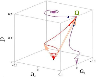
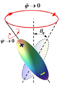
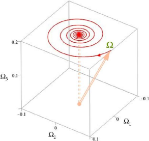
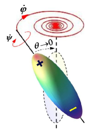
Figure 1: Left – hodograph and its projections onto coordinate planes of angular velocity $\boldsymbol{\Omega}$ in the proper reference frame of the axially-symmetric polarized spinning-top according to the truncated ALE equations; the rate of principal moments of inertia: $I_{3}/I_{1}=2/5$; initial angular velocity: $\boldsymbol{\Omega}_{0}=\{0,0.1,0.2\}$ in $1/\tau$ units. Right – qualitative behavior of the spinning-top in space: inclination angle is constant $\theta_{0}$, and speeds of precession $\dot{\varphi}$ and proper rotation $\dot{\psi}$ decrease in asymptotics $t\to\infty$ to zero as $\sim 1/\sqrt{t}$.

Figure 2: The same as in figure 1, but according to the reduced ALE equations: the inclination angle $\theta$ in asymptotics $t\to\infty$ tends exponentially to zero while the proper rotation speed tends to the constant $\Omega_{3}$.

According to [11, § 75], the equation (2.2) is derived from the expression for the force of the dipole radiation reaction, i.e., the Abraham-Lorentz expression generalized for a system of several charges.

Since the Abraham-Lorentz equation is generally accepted, the balance equation (2.2) should be preferred. Let us note that the authors of the textbook [11] apparently considered this equation as an intermediate formula (unnumbered in [11, § 75]), which is further reduced to the previously obtained (Problem 2 in [11, § 72]) equation (2.1) by neglecting the Schott term. It was noted that this step is admissible provided the motion is stationary (but in [11, § 75] the nearly stationary motion apparently implied). In the present case a free symmetric Euler spinning-top makes certainly a stationary motion but the taking the radiation reaction into account without the Schott term and with it leads to a nearly stationary motions with quite different final states of the top. Once the balance equation (2.2) is plausible, then there is something wrong with the equation (2.1) or its usage.

Similarly to the Larmor formula, the balance equation (2.1) was derived in [11] (§ 72, Problem 2) by means of an integration of the angular momentum flux over a sphere of some radius $R_{0}$ surrounding a system of charges.

According to one common interpretation [5], the Schott energy (and the Schott angular momentum in our instance) of nonrelativistic system (which is the case) is not present in the Larmor formula (here – in eq. (2.1)) because it is localized somewhere close to charges, i.e., deep under the integration sphere.

But the neglect of the Schott term leads in our case to an irreparable “loss” of the remnant energy $E=I_{3}\Omega_{3}^{2}/2$ and the angular momentum $L_{3}=I_{3}\Omega_{3}$ via radiation across the integration surface. Thus this interpretation does not clarify the current problem.

According to another, later interpretation by A. Singal [7], there is no need to attribute spatial localization and even physical essence to the Schott energy. When considering the Larmor formula one usually does not take into account the fact that although the radius of the integration sphere $R_{0}$ falls out of the final formula (see, for example, (67.8) or (67.9) in [11]), its right-hand side refers to the moment of time delayed by $R_{0}/c$ that is the value required to reach by electromagnetic signal the sphere from its center.

The recalculation of the Larmor formula to “real” time, carried out with the spherical-shell model of a charged particle [7], reproduces the Schott term in this formula, and thus removes the inconsistency of the energy balance equations. The recalculation, however, refers to the electromagnetic structure of charged particles, and hence that structure may be considered as a carrier of the acceleration-dependent Schott energy. This interpretation following from Singal’s calculations disagrees with his own interpretation but is consistent with the conception of charged particles as extended, composite, and therefore non-rigid objects due to their electromagnetic structure [4].

In the Appendix, a similar recalculation is performed in the angular momentum balance equation of a charged particle. By this it is approved the correctness of the formula (2.2) and the incorrect application of the formula (2.1).

Appendix. On interpretation of the Shott term in the angular momentum balance equation.

Following the Singal’s calculations [7] (but with different interpretation in mind), we present the charged particle as a sphere of small radius $r_{0}$, and its mass as the sum of the “bare” mass $m_{0}$ and the electromagnetic mass $m_{\rm em}=2q^{2}/(3c^{2}r_{0})$. Then the equation of motion can be represented in such a way

$$\frac{{\rm d}{}\,}{{\rm d}{t}\,}\big{\{}m_{0}{\boldsymbol{v}}(t)+m_{\rm em}{\boldsymbol{v}}(t-r_{0}/c)\big{\}}+O(r_{0})=\boldsymbol{F}_{\!\!\rm ex}(t),$$ (A.1)

that in the limit $r_{0}\to 0$ the total mass $m=m_{0}+m_{\rm em}$ keeps finite, and the equation (A.1) goes into (2.5). The 1st term in curly braces represents a “bare” contribution in the particle momentum, the 2nd one is a contribution of its electromagnetic “fur”; the later perceives a change of position, velocity etc. with delay because of a finite size of the particle.

Hereafter the moment of time $t$ as the argument of physical quantities will be omitted, and the retarded moment of time $t-r_{0}/c$ will be denoted by index “ret”.

Let us multiply vectorially $\boldsymbol{r}$ by equation (A.1), use the Taylor series expansion up to the 1st order, $\boldsymbol{r}\simeq[\boldsymbol{r}]_{\rm ret}+[\dot{\boldsymbol{r}}]_{\rm ret}r_{0}/c$, and rearrange terms:

$$\frac{{\rm d}{}\,}{{\rm d}{t}\,}\big{\{}m_{0}{\boldsymbol{r}}\times{\boldsymbol{v}}+m_{\rm em}[{\boldsymbol{r}}\times{\boldsymbol{v}}]_{\rm ret}\big{\}}+O(r_{0})=-\frac{2q^{2}}{3c^{3}}[{\boldsymbol{v}}\times\dot{\boldsymbol{v}}]_{\rm ret}.$$ (A.2)

This equation clears up a meaning of the equation (2.8): on the left in curly braces is a total angular momentum of the particle consisting of “bare” and electromagnetic contributions. On the right is a result of the integration of the angular momentum flux over the sphere which radius cannot be smaller than $r_{0}$ (hence the delayed argument). In the limit $r_{0}\to 0$ we have

$$\lim_{r_{0}\to 0}m_{\rm em}\big{\{}[{\boldsymbol{r}}\times{\boldsymbol{v}}]_{\rm ret}-{\boldsymbol{r}}\times{\boldsymbol{v}}\big{\}}=-\tau_{0}\dot{\boldsymbol{L}}\equiv-{\boldsymbol{L}}_{\rm S},$$ (A.3)

where $\tau_{0}=2q^{2}/(3mc^{3})$. This reduces the equation (A.2) to (2.6). Obviously, one can treat in a similar manner the relation of the balance equations (2.1) and (2.2) for a system of charges.

References

- [1] Eager D, Pendrill A M and Reistad N 2016 Beyond velocity and acceleration: jerk, snap and higher derivatives Eur. J. Phys. 37 065008
- [2] Schott G 1912 Electromagnetic radiation and the mechanical reactions arising from it (Cambridge University Press)
- [3] Eriksen E and Grøn Ø 2007 On the energy and momentum of an accelerated charged particle and the sources of radiation Eur. J. Phys. 28 401-407
- [4] Rowland D R 2010 Physical interpretation of the Schott energy of an accelerating point charge and the question of whether a uniformly accerelaticg charge radiates Eur. J. Phys. 31 1037-1051
- [5] Grøn Ø 2011 The significance of the Schott energy for energy-momentum conservation of a radiating charge obeying the Lorentz–Abraham–Dirac equation Am. J. Phys. 79 115–122
- [6] Singal A K 2016 Poynting flux in the neighbourhood of a point charge in arbitrary motion and radiative power losses Eur. J. Phys. 37 045210
- [7] Singal A K 2016 Compatibility of Larmor’s formula with radiation reaction for an accelerated charge Found. Phys. 46 554–574
- [8] Jackson J D 1999 Classical electrodynamics 3rd ed (Wiley)
- [9] Panofsky W K H and Phillips M 1962 Classical electricity and magnetism 2nd ed Dover Books on Physics (Dover Publications)
- [10] Griffiths D J 2017 Introduction to Electrodynamics 4th ed (Cambridge University Press)
- [11] Landau L D and Lifshitz E M 1987 The clasical theory of fields 4th ed Course of theoretical physics vol 2 (Butterworth-Heinemann)
- [12] Iro H 2016 A Modem Approach to Classical Mechanics 2nd ed (Singapore: World Scientific)
- [13] Nakamura T 2020 On the Schott term in the Lorentz-Abraham-Dirac equation Quantum Beam Sci. 4 34
- [14] Singal A K 2016 Radiation reaction and the pitch angle changes for a charge undergoing synchrotron losses MNRAS 458 2303–2306
- [15] de Groot S R and Suttorp L G 1972 Foundations of electrodynamics (Amsterdam: North-Holland Publ. Co.)
- [16] Rohrlich F 1990 Classical charged particles: foundations of their theory (New York: Addison-Wesley)
- [17] Yaremko Yu and Tretyak V 2012 Radiation reaction in classical field theory: basics, concepts, methods (Saarbrücken: LAP)
- [18] Dirac P A M 1938 Classical theory of radiating electrons Proc. R. Soc. Lon. Ser-A 167 148–169
- [19] Lorentz H A 1952 The Theory of Electrons: And its Applications to the Phenomena of Light and Radiant Heat 2nd ed (New York: Dover Publications, Inc.)
- [20] Reimann R, Doderer M, Hebestrait E, Diehl R, Frimmer M, Windey D, Tebbenjohanns F and Novotny L 2018 Ghz rotation of an optically trapped nanoparticle in vacuum Phys. Rev. Lett 121 033602
- [21] Ahn J, Xu Z, Bang J, Ju P, Gao X and Li T 2020 Ultrasensitive torque detection with an optically levitated nanorotor Nat. Nanotechnol. 15 89–95
- [22] Shanbhag S and Kotov N A 2006 On the origin of a permanent dipole moment in nanocrystals with a cubic crystal lattice: Effects of truncation, stabilizers, and medium for CdS tetrahedral homologues Psys. Chem. Lett. B 110 12211–12217
- [23] Frka-Petesic B, Jean B and Heux L 2014 First experimental evidence of a giant permanent electric-dipole moment in cellulose nanocrystals Europhys. Lett. 107 28006
- [24] Masuhara H, Nakanishi H and Sasaki K 2003 Single Organic Nanoparticles (Berlin: Springer-Verlag) section 29.5
- [25] Duviryak A 2020 Rotary dynamics of the rigid body electric dipole under the radiation reaction Eur. Phys. J. D 74 189
- [26] Rajeev S G 2008 Exact solution of the Landau Lifshitz equations for a radiating charged particle in the Coulomb potential Ann. Phys. 323 2654-2661
- [27] Vogel M 2018 Particle confinement in Penning traps. An introduction Springer series on Atomic, Optical, and Plasma Physics vol 100 (Cham: Springer)
- [28] Yaremko Y, Przybylska M and Maciejewski A J 2015 Dynamics of a relativistic charge in the Penning trap Chaos 25 053102
- [29] Pauli W 1958 Theory of relativity (London: Pergamon Press)
- [30] Xu C, Tao J and Wu X 2004 Post-Newtonian quasirigid body Phys. Rev. D 69(2) 024003