Explicit examples of resonances for Anosov maps of the torus

Abstract

In [23] Slipantschuk, Bandtlow and Just gave concrete examples of Anosov diffeomorphisms of $\mathbb{T}^{2}$ for which their resonances could be completely described. Their approach was based on composition operators acting on analytic anisotropic Hilbert spaces. In this note we present a construction of alternative anisotropic Hilbert spaces which helps to simplify parts of their analysis and gives scope for constructing further examples.

1 Introduction

In the study of chaotic diffeomorphisms, a natural class of examples are Anosov diffeomorphisms. In fact, it is the principle of the Cohen-Gallavotti chaotic hypothesis that chaotic behaviour can be understood through the dynamics of Anosov systems [8].

The study of Anosov dynamics is advanced by understanding various dynamical quantities, including the resonances. Given a map $T$, its resonances comprise a sequence (finite or converging to zero) of distinct complex numbers $(\rho_{n})_{n=1}^{\infty}$, which give all possible exponential decay rates for the correlation function

$$\int f\circ T^{m}g\;d\mu-\int f\,d\mu\int g\,d\mu,\qquad m\geq 0,$$

for all (sufficiently smooth) observables $f$ and $g$, and where $\mu$ is the SRB measure (see, e.g., [25] for an account of the SRB measure, and [3, Theorem 7.11] for a precise statement).

Until recently, the only examples for which these resonances are completely known were given by linear hyperbolic diffeomorphisms (which represent all hyperbolic diffeomorphisms of tori up to isotopy [13]). These examples, including the Arnol’d CAT map $B_{0}:\mathbb{T}^{2}\to\mathbb{T}^{2}$ of [2],

$$B_{0}:\binom{a}{b}\mapsto\begin{pmatrix}2&1\\ 1&1\end{pmatrix}\binom{a}{b}\mod 1,$$

have only the trivial resonances ($0$ and $1$). On the other hand, Adam in [1] showed that generic small perturbations of these linear diffeomorphisms yield at least one non-trivial resonance. In the context of pseudo-Anosov surface homeomorphisms a description for resonances of linear pseudo-Anosov maps was recently given in [15]. However, of particular interest to us are the very interesting examples are given in the striking work [23] of Slipantshuk, Bandtlow and Just. More explicitly, they provide a family of Anosov diffeomorphisms, $(B_{\lambda})$, perturbing $B_{0}$ above, for which the resonances $(\rho_{n})_{n}$ (with respect to real analytic functions $f$ and $g$) are infinite and explicitly known:

$$\{\rho_{n}\}_{n=1}^{\infty}\subset\{0,1\}\cup\{\lambda^{n},\overline{\lambda}^{n}\,:\,n\in\mathbb{N}\};$$

where $\lambda$ is an arbitrary complex parameter with $|\lambda|<1$. The resonances of an Anosov map $T$ are calculated as the eigenvalues of its composition operator, $\mathcal{C}_{T}:f\mapsto f\circ T$, or its adjoint, the transfer operator, acting quasi-compactly on a suitable Banach space. In particular, we can rewrite the correlation function as $\int\mathcal{C}_{T}^{m}(f)g\,d\mu-\int f\,d\mu\int g\,d\mu$ for $m\geq 0$ and then deduce that, for any $\varepsilon>0$, there exist polynomials $\{p_{n}\}_{n=1}^{N}$ such that

$$\int f\circ T^{m}g\;d\mu-\int f\,d\mu\int g\,d\mu=\sum_{n=1}^{N}p_{n}(m)\rho_{n}^{m}+\mathcal{O}\left(\varepsilon^{m}\right),\qquad m\geq 0$$

(where the degree of $p_{n}$ is determined by the multiplicity of $\rho_{n}$). The ambient spaces, known as anisotropic spaces, have to be tailored to the diffeomorphism $T$ and their construction is non-trivial. (A description of the myriad anisotropic spaces seen in the literature are given an overview in [11] and a more thorough account in the survey [4].)

In this article, inspired by [23], we give a new account of the resonances of $B_{\lambda}$ and other related examples. In particular, rather than using the spaces in [23] (which are, in turn, based on [14]) we introduce a new family of anisotropic Hilbert spaces using what we call a degree function. The main advantage of this construction is that it allows us to simplify the technical analysis substantially. Moreover, this approach also allows us to prove new results on the resonances in greater generality, which we illustrate by two other families, $T_{\lambda}$ and $T_{\lambda}\circ T_{\mu}$ in §2 and §3, respectively, where throughout this note, $\lambda$ and $\mu$ will denote complex parameters with $|\lambda|,|\mu|<1$. The results on the former family appear to be new. The resonances of the latter family are studied empirically in an appendix of [23], but we will give a rigorous proof.

We recall that a diffeomorphism $T:\mathbb{T}^{2}\to\mathbb{T}^{2}$ is Anosov if there exists a continuous $DT$-invariant splitting of the tangent space $\mathcal{T}_{\ast}\mathbb{T}^{2}=E^{s}\oplus E^{u}$ such that there exists $C>0$ and $0<\lambda<1$ such that $\|DT^{n}|E^{s}\|\leq C\lambda^{n}$ and $\|DT^{-n}|E^{u}\|\leq C\lambda^{n}$, for all $n\geq 0$. Although the examples in this note are all Anosov, the proofs of the results are self-contained and don’t depend on general properties of Anosov diffeomorphisms.

1.1 Contents of this note

In §2, §3 and §4, respectively, we follow the general strategy of [23] for three different families of Anosov maps $B_{\lambda}$, $T_{\lambda}$ and $T_{\lambda}\circ T_{\mu}$:

1. For each family, we exhibit a family of anisotropic Hilbert spaces, and show that these can be chosen to contain any pair of functions analytic on a neighbourhood of the torus.

2. We also show that the composition operator acts compactly on these spaces (so that its spectrum gives the resonances of the map).

3. Finally, we calculate the spectrum of this operator using a convenient, block-triangular matrix form.

These results appear in the thesis of the second author [20].

2 The resonances of $B_{\lambda}$

The family of Anosov diffeomorphisms $B_{\lambda}$ (for $|\lambda|<1$) studied in [23] are given by so-called two-dimensional Blaschke products, originally introduced in more generality by [18], where some ergodic properties were established (see also [17]). More explicitly, considering

$$\mathbb{T}^{2}=\mathbb{T}\times\mathbb{T}\subset\mathbb{C}\times\mathbb{C},\hbox{ where }\mathbb{T}:=\{z\in\mathbb{C}:|z|=1\},$$

we have the following definition.

Definition 2.1 ($B_{\lambda}$).

Let $B_{\lambda}:\mathbb{T}^{2}\to\mathbb{T}^{2}$ be given by

$$B_{\lambda}:(z,w)\mapsto\left(\left(\frac{z+\lambda}{1+\overline{\lambda}z}\right)zw,\left(\frac{z+\lambda}{1+\overline{\lambda}z}\right)w\right).$$

This family of maps analytically perturbs the standard Arnol’d CAT map, represented on $\mathbb{T}^{2}$ by $B_{0}:(z,w)\mapsto(z^{2}w,zw).$ The maps $B_{\lambda}$ are Anosov and area-preserving for all $\lambda$ satisfying $|\lambda|<1$ [20, 23]. In particular, the resonances are well-defined and the SRB measure is just the unit area measure.

We will reprove the following result on the resonances of $B_{\lambda}$. This is the main result of [23], and we provide a new, simplified perspective.

Theorem 2.2 (Slipantschuk, Bandtlow and Just).

Given $\lambda$ with $|\lambda|<1$, there exists an area preserving Anosov diffeomorphism for which the resonances with respect to analytic functions $f,g:\mathbb{T}^{2}\to\mathbb{R}$ take the form

$$\{0,1\}\cup\{\lambda^{m},\,\overline{\lambda}\vphantom{\lambda}^{m}\,:\,m\in\mathbb{N}\}.$$

Moreover, each non-zero value is simple, up to coincidences in value, and is otherwise semi-simple (i.e., the algebraic and geometric multiplicities coincide) of multiplicity two.

The proof is based on the construction of a (non-canonical) Hilbert space, $\mathcal{H}_{a}$, consisting of distributions on the torus, on which the composition operator $\mathcal{C}_{B_{\lambda}}:f\mapsto f\circ B_{\lambda}$ acts compactly and has the spectrum described in the theorem. We now describe the construction of the new Hilbert spaces $\mathcal{H}_{a}$ we will use in the next section.

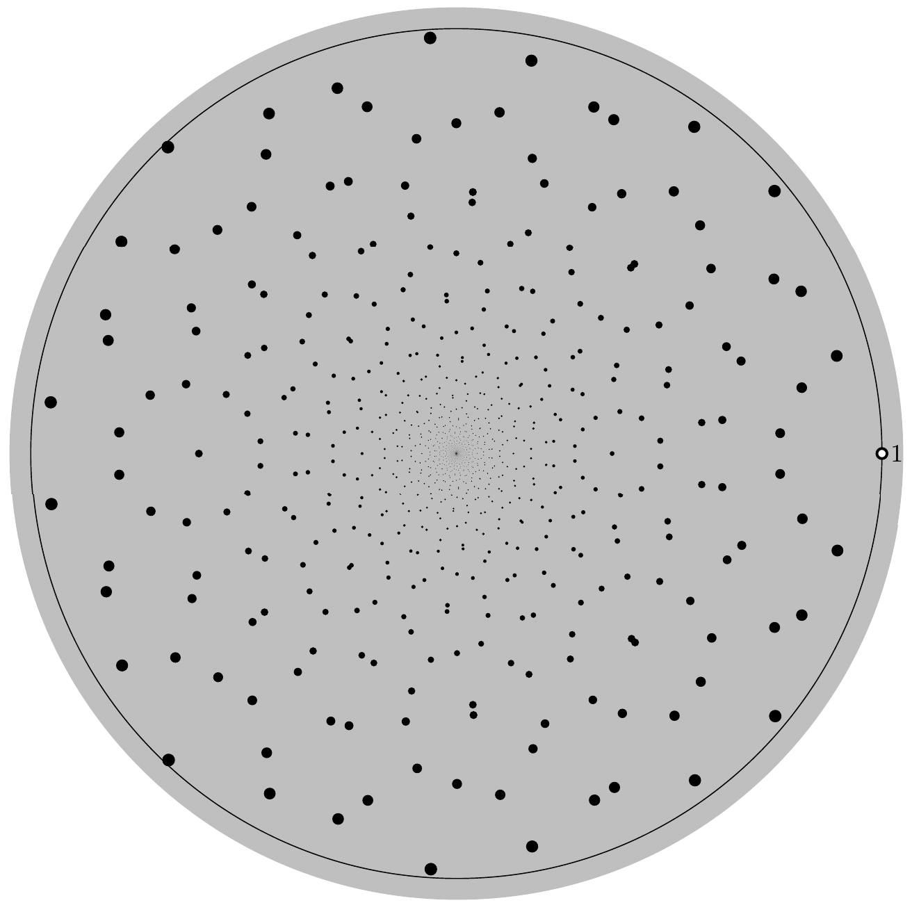
Figure 1: The spectrum of $\mathcal{C}_{B_{\lambda}}$, for $\lambda=0.99e^{37i\pi/50}$.

2.1 The Hilbert space $\mathcal{H}_{a}$

All the Hilbert spaces discussed in this note are constructed using the following basic method. Consider a complex Hilbert space $\mathcal{H}$ which has as an orthogonal basis the collection of monomials $\{e_{m,n}\}_{(m,n)\in\mathbb{Z}^{2}}$ given by

$$e_{m,n}:(z,w)\mapsto z^{m}w^{n}.$$

Denoting $\langle\cdot,\cdot\rangle$ and $\|\cdot\|$ for the inner product and norm on $\mathcal{H}$ respectively, we have

$$\left\langle\sum_{(m,n)\in\mathbb{Z}^{2}}b_{m,n}e_{m,n},\sum_{(m,n)\in\mathbb{Z}^{2}}c_{m,n}e_{m,n}\right\rangle=\sum_{(m,n)\in\mathbb{Z}^{2}}b_{m,n}\overline{c_{m,n}}\,\|e_{m,n}\|^{2}$$

and

$$\Big{\|}\sum_{(m,n)\in\mathbb{Z}^{2}}b_{m,n}e_{m,n}\;\Big{\|}^{2}=\sum_{(m,n)\in\mathbb{Z}^{2}}|b_{m,n}|^{2}\|e_{m,n}\|^{2}.$$

We define $\mathcal{H}$ to comprise those series with finite $\|\cdot\|$ norm:

$$\mathcal{H}=\left\{\sum_{(m,n)\in\mathbb{Z}^{2}}b_{m,n}e_{m,n}\;\bigg{|}\;b_{m,n}\in\mathbb{C},\ \sum_{(m,n)\in\mathbb{Z}^{2}}|b_{m,n}|^{2}\|e_{m,n}\|^{2}<\infty\right\}.$$

In particular, $\mathcal{H}$ is completely characterised by the values $\|e_{m,n}\|$ which we call the weights.

Remark 2.3.

For any $a>0$, classical examples of such spaces include the Sobolev space of $a$-times weakly differentiable functions [24, p.42], which can be defined by $\|e_{m,n}\|=\big{(}|m|+|n|+1\big{)}^{a}.$ Unfortunately, these spaces do not suffice for our purposes.

To obtain the required properties for the composition operator acting on the Hilbert space $\mathcal{H}$, we need to define the weights in an anisotropic manner. In particular, taking limits along rays based at the origin, these weights decay to zero in some directions and diverge to infinity in others, and it is this behaviour which characterises the anisotropic nature of the space.

Remark 2.4.

In [23], after [14], the authors base these weights on the eigenvectors of the map $B_{0}$: i.e., for $a>0$,

$$\|e_{m,n}\|=\exp\left(-a\left|\frac{\sqrt{5}+1}{2}m+n\right|+a\left|\frac{1-\sqrt{5}}{2}m+n\right|\right).$$ (1)

These are a particular instance of the anisotropic spaces introduced in greater generality by Faure and Roy in [14] and also used by Adam [1]. The two essential properties of such Hilbert spaces are that the composition operator $\mathcal{C}_{B_{\lambda}}$ acts compactly on them, and that $a>0$ can be chosen so that the space contains any given pair of functions analytic on a neighbourhood of the torus.

Assuming it acts compactly, the computation of the spectrum of the composition operator acting on $\mathcal{H}$ above is to some extent independent of the specific weights used. We therefore present simple alternative weightings, yielding new families of anisotropic Hilbert spaces. These spaces will be particularly simple for $B_{\lambda}$; although we will need a small adjustment when we consider $T_{\lambda}$ in the next section.

The definition of the spaces $\mathcal{H}_{a}$, appropriate to $B_{\lambda}$, make use of the degree function $\deg_{1}$, which we now give.

Definition 2.5 ($\deg_{1}$, $\|\cdot\|_{a}$, $\mathcal{H}_{a}$).

Let $\deg_{1}:\mathbb{Z}^{2}\to\mathbb{Z}$ be given by

$$\deg_{1}(m,n):=\operatorname{sign}(mn)\big{(}|m|+|n|\big{)},$$

where

$$\hbox{\rm sign}(k)=\begin{cases}\phantom{-}1,&\text{if }k\geq 0;\\ -1,&\text{if }k<0.\end{cases}$$

We define, for $a>0$,

$$\|e_{m,n}\|_{a}:=e^{-a\deg(m,n)}.$$

As described above, we let $\mathcal{H}_{a}$ be the space of series in $e_{m,n}$ with finite $\|\cdot\|_{a}$ norm:

$$\bigg{\|}\sum_{(m,n)\in\mathbb{Z}^{2}}b_{m,n}e_{m,n}\;\bigg{\|}^{2}_{a}:=\sum_{(m,n)\in\mathbb{Z}^{2}}|b_{m,n}|^{2}e^{-2a\deg_{1}(m,n)}.$$

Figure 2 shows some level sets of $\deg_{1}$.

Figure 2: The level sets of $\deg_{1}:\mathbb{Z}^{2}\to\mathbb{Z}$. Here, $D_{n}$ denotes ${\deg_{1}}^{-1}(n)$.

The benefits of using $\mathcal{H}_{a}$ over the original family of anisotropic spaces defined by (1) can be summarized as follows. The proofs for compactness of the composition operators $\mathcal{C}:\mathcal{H}_{a}\to\mathcal{H}_{a}$ and the inclusion of analytic functions in $\mathcal{H}_{a}$ appear simpler and more direct. Secondly, the construction permits more flexibility. (For example, it works also for the families $B_{\lambda,K}$ in the final section). Finally, there is a clearer link between the structure of the space and the simple (block-triangular) form for the matrix of the operator.

The following result shows that any pair of analytic functions on a neighbourhood of the torus will be contained in some $\mathcal{H}_{a}$, allowing us to equate the resonances of $B_{\lambda}$ with the spectrum described in Theorem 2.2.

Proposition 2.6.

Let $a>0$ and suppose that $f$ is an analytic function on a neighbourhood of the poly-annulus

$$P_{a}:=\left\{(z,w)\in\mathbb{C}^{2}\;\big{|}\;e^{-a}\leq|z|\leq e^{a},\ e^{-a}\leq|w|\leq e^{a}\right\}.$$

Then $f\in\mathcal{H}_{a}$. In particular, every function analytic on a neighbourhood of $\mathbb{T}^{2}$ is contained in $\mathcal{H}_{a}$ for all sufficiently small $a$.

Proof.

Fix $a$ and let $f\in\mathcal{H}_{a}$. By construction, the Laurent series for $f$ converges absolutely on $P_{a}$. In particular, writing this expansion as

$$f(z,w)=\sum_{(m,n)\in\mathbb{Z}^{2}}b_{m,n}z^{m}w^{n},$$ (2)

we have, by definition of $\|\cdot\|_{a}$,

$$\|f\|_{a}^{2}=\sum_{(m,n)\in\mathbb{Z}^{2}}|b_{m,n}|^{2}\,e^{-2a\deg_{1}(m,n)}\leq\sum_{(m,n)\in\mathbb{Z}^{2}}|b_{m,n}|^{2}\,e^{2a(|m|+|n|)},$$

which we want to show is finite. Note that

$$\sum_{m,n}|b_{m,n}|e^{a(|m|+|n|)} \leq\sum_{m,n}|b_{m,n}|\left(e^{a(m+n)}+e^{a(m-n)}+e^{a(n-m)}+e^{-a(m+n)}\right)$$

is finite, since (2) converges absolutely for all $(z,w)\in P_{a}$: i.e., the sums

$$\sum_{m,n}|b_{m,n}|e^{a(m+n)},\qquad\sum_{m,n}|b_{m,n}|e^{a(m-n)},$$

$$\sum_{m,n}|b_{m,n}|e^{a(n-m)},\qquad\sum_{m,n}|b_{m,n}|e^{-a(m+n)}$$

are each finite, since $(e^{\pm a},e^{\pm a})\in P_{a}$. In particular, the left hand side is square-summable, and hence $f\in\mathcal{H}_{a}$ as required. ∎

2.2 $\mathcal{C}_{B_{\lambda}}$ is Hilbert-Schmidt

Since the composition operators can be understood through their action on the basis functions we need us estimate the corresponding Taylor series coefficients that appear.

2.2.1 Estimates on Taylor coefficients

The following definition will be used throughout.

Definition 2.7 ($\alpha_{m,k}$).

For all $m\in\mathbb{N}_{0}$, the following expansion converges uniformly on every disk of radius less than $|\lambda|^{-1}$:

$$\left(\frac{z+\lambda}{1+\overline{\lambda}z}\right)^{m}=\sum_{k=0}^{\infty}\alpha_{m,k}z^{k}.$$ (3)

The complex coefficients $\alpha_{m,k}$ can be formulated explicitly using the Cauchy integral formula or Newton’s identity. In particular, we have $\alpha_{m,0}=\lambda^{m}$ for all $m\in\mathbb{N}_{0}$, and $\alpha_{0,k}=0$ for all $k\in\mathbb{N}$.

Using symmetry, one also obtains a related Taylor expansion about $\infty$ for $m\leq-1$:

$$\left(\frac{z+\lambda}{1+\overline{\lambda}z}\right)^{m}=\left(\frac{z^{-1}+\overline{\lambda}}{1+\lambda z^{-1}}\right)^{-m}=\sum_{k=0}^{\infty}\overline{\alpha_{-m,k}}z^{-k}.$$ (4)

For simplicity, we adopt the notation that $\alpha_{-m,k}=\overline{\alpha_{m,k}}$ for all $m$ and $k$.

As observed in [23] the proof of compactness of $\mathcal{C}_{B_{\lambda}}$ reduces to estimating sums of the form

$$\sum_{k=0}^{\infty}|\alpha_{m,k}|^{2}e^{-2ak}$$

for each $m\in\mathbb{Z}$, and for $a>0$ fixed. In Lemma 2.3 of [23] this was derived using the Cauchy integral formula. We now present an alternative estimate, which has the advantages of being direct, simple and explicit.

Lemma 2.8.

For all $\lambda$ and $a>0$,

$$M_{a,\lambda}:=\max_{|z|=e^{-2a}}\left|\frac{z+\ \lambda}{1+\overline{\lambda}z}\right|<1.$$ (5)

Moreover, $M_{a,\lambda}$ satisfies, for all $m\in\mathbb{Z}$,

$$\sum_{k=0}^{\infty}|\alpha_{m,k}|^{2}e^{-2ak}\leq M_{a,\lambda}^{|m|}.$$

Proof.

Since $|\alpha_{m,k}|=|\alpha_{-m,k}|$, it suffices to assume $m\geq 0$. Since

$$\frac{1}{2\pi}\int_{\mathbb{T}^{1}}z^{k-j}\;|dz|:=\frac{1}{2\pi}\int_{0}^{2\pi}e^{i(k-j)\theta}d\theta=\begin{cases}1,&\hbox{ if }k=j;\cr 0,&\hbox{ if }k\neq j;\cr\end{cases}$$

we have the following, exchanging sums and integral:

$$\sum_{k=0}^{\infty}|\alpha_{m,k}|^{2}e^{-2ak} =\frac{1}{2\pi}\sum_{k=0}^{\infty}\sum_{j=0}^{\infty}\alpha_{m,k}\overline{\alpha_{m,j}}e^{-2ak}\int_{\mathbb{T}^{1}}z^{k}z^{-j}\;|\mathrm{d}z|$$

$$=\frac{1}{2\pi}\sum_{k=0}^{\infty}\sum_{j=0}^{\infty}\alpha_{m,k}\overline{\alpha_{m,j}}\int_{\mathbb{T}^{1}}(ze^{-2a})^{k}z^{-j}\;|\mathrm{d}z|$$

$$=\frac{1}{2\pi}\int_{\mathbb{T}^{1}}\sum_{k=0}^{\infty}\alpha_{m,k}(ze^{-2a})^{k}\sum_{j=0}^{\infty}\overline{\alpha_{m,j}}z^{-j}\;|\mathrm{d}z|$$

$$=\frac{1}{2\pi}\int_{\mathbb{T}^{1}}\left(\frac{ze^{-2a}+\lambda}{1+\overline{\lambda}e^{-2a}z}\right)^{m}\left(\frac{z+\lambda}{1+\overline{\lambda}z}\right)^{-m}\;|\mathrm{d}z|,$$

and a uniform estimate on this integral gives

$$\sum_{k=0}^{\infty}|\alpha_{m,k}|^{2}e^{-2ak} \leq\max_{|z|=1}\left|\frac{ze^{-2a}+\lambda}{1+\overline{\lambda}e^{-2a}z}\right|^{m}{\underbrace{\left|\frac{z+\lambda}{1+\overline{\lambda}z}\right|}_{=1}}^{-m}$$

$$=\max_{|ze^{2a}|=1}\left|\frac{z+\lambda}{1+\overline{\lambda}z}\right|^{m}=M_{a,\lambda}^{m},$$

which proves (5). Finally, elementary calculus shows that

$$M_{a,\lambda}=\frac{|\lambda|+e^{-2a}}{1+e^{-2a}|\lambda|},$$

leading to $M_{a,\lambda}<1$. ∎

2.2.2 Application to $\mathcal{C}_{B_{\lambda}}$

The previous lemma suffices to prove the following property for the composition operator $\mathcal{C}_{B_{\lambda}}$. This immediately implies compactness [9, p.267].

Definition 2.9 (Hilbert-Schmidt, $\|\cdot\|_{\text{HS}}$).

The Hilbert-Schmidt norm of an operator $\mathcal{C}:\mathcal{H}\to\mathcal{H}$ acting on a separable Hilbert space $\mathcal{H}$, for any orthogonal basis $\{e_{i}\}_{i\in\mathcal{I}}$ of $\mathcal{H}$, is given by

$$\|\mathcal{C}\|_{\text{\emph{HS}}}^{2}=\sum_{i\in\mathcal{I}}\left(\frac{\|\mathcal{C}(e_{i})\|}{\|e_{i}\|}\right)^{2}.$$

We say that $\mathcal{C}$ is Hilbert-Schmidt if it has finite Hilbert-Schmidt norm. Note that the norm is independent of the choice of basis [9, p.267].

We now show that $\mathcal{C}_{B_{\lambda}}$ has this property.

Proposition 2.10.

For all $a>0$, $\mathcal{C}_{B_{\lambda}}:\mathcal{H}_{a}\to\mathcal{H}_{a}$ is Hilbert-Schmidt.

The proof of this proposition uses the following simple lemma.

Lemma 2.11.

For all $(m,n)\in\mathbb{Z}^{2}$, whenever $n\neq 0$,

$$\deg_{1}(m+\operatorname{sign}(n),n)\geq\deg_{1}(m,n)+1.$$ (6)

Similarly, $\deg_{1}(m,\operatorname{sign}(m)+n)\geq\deg_{1}(m,n)+1$ whenever $m\neq 0$.

Although the lemma is quite intuitive (see Figure 2) we give an analytic proof for completeness.

Proof.

We only prove the first inequality, since the second follows by symmetry. We prove it in three cases:
Case 1: $mn\geq 0$. Then $(m+\operatorname{sign}(n))n=mn+|n|\geq 0$ and thus

$$\deg_{1}(m+\operatorname{sign}(n),n)=\operatorname{sign}\big{(}\underbrace{|m+\operatorname{sign}(n)|}_{{|m|+1}}+|n|\big{)} =|m|+|n|+1$$

$$=\deg_{1}(m,n)+1.$$

Case 2: $mn<0$ and $|m|>1$. Then $mn+|n|<0$ and thus

$$\deg_{1}(m+\operatorname{sign}(n),n)=-\big{(}\underbrace{|m+\operatorname{sign}(n)|}_{{|m|-1}}+|n|\big{)} =1-|m|-|n|$$

$$=\deg_{1}(m,n)+1.$$

Case 3: $mn<0$ and $|m|=1$. The two hypotheses give $mn+|n|=0$ and thus $\deg_{1}(m+\operatorname{sign}(n),n)\geq 0$, whereas $mn<0$ implies that $\deg_{1}(m,n)\leq-1$, completing the proof. ∎

We now return to the proof of Proposition 2.10.

Proof of Proposition 2.10 .

Fix $\lambda$ and $a>0$, and consider $\mathcal{C}_{B_{\lambda}}(e_{m,n})$. The Taylor expansions of (3) and (4) give

$$e_{m,n}\big{(}B_{\lambda}(z,w)\big{)} =\left(\frac{z+\lambda}{1+\overline{\lambda}z}\right)^{m+n}z^{m}w^{m+n}$$

$$=\begin{cases}\rule{0.0pt}{20.0pt}\displaystyle\sum_{k=0}^{\infty}\alpha_{m+n,k}z^{m+\sigma k}w^{m+n},&\text{if }m+n\neq 0;\\ \qquad z^{m}w^{m+n},&\text{if }m+n=0;\end{cases}$$

where we denote $\sigma=\hbox{\rm sign}(m+n)$. That is,

$$\mathcal{C}_{B_{\lambda}}(e_{m,n})=\begin{cases}\displaystyle\sum_{k=0}^{\infty}\alpha_{m+n,k}\,e_{m+\sigma k,m+n},&\text{if }m+n\neq 0;\\ \qquad e_{m,m+n}=e_{m,0},&\text{if }m+n=0.\end{cases}$$ (7)

Consider the case that $m+n\neq 0$. To estimate

$$\left(\frac{\|\mathcal{C}_{B_{\lambda}}(e_{m,n})\|_{a}}{\|e_{m,n}\|_{a}}\right)^{2} =\sum_{k=0}^{\infty}|\alpha_{m+n,k}|^{2}\left(\frac{\|e_{m+\sigma k,m+n}\|_{a}}{\|e_{m,n}\|_{a}}\right)^{2},$$ (8)

we first bound

$$\frac{\|e_{m+\sigma k,m+n}\|_{a}}{\|e_{m,n}\|_{a}}=\exp\left[-a\big{(}\deg_{1}(m+\sigma k,m+n)-\deg_{1}(m,n)\big{)}\right],$$ (9)

for each $k\in\mathbb{N}_{0}$. To this end, we apply Lemma 2.11 in two different ways. Firstly, since $m+n\neq 0$, applying the lemma $k$ times gives

$$\deg_{1}(m+\sigma k,m+n)=\deg_{1}\big{(}m+\sigma k,m+n\big{)}\geq\deg_{1}(m,m+n)+k.$$

Secondly, applying the lemma $|m|$ times to the right hand side gives

$$\deg_{1}(m,m+n)=\deg_{1}\big{(}m,|m|\hbox{\rm sign}(m)+n\big{)}\geq\deg_{1}(m,n)+|m|$$

(if $m=0$, the inequality is trivial). That is,

$$\deg_{1}(m+\sigma k,m+n)\geq\deg_{1}(m,n)+|m|+k.$$ (10)

Thus, by (9),

$$\frac{\|e_{m+\sigma k,m+n}\|_{a}}{\|e_{m,n}\|_{a}}\leq e^{-a\big{(}|m|+k\big{)}}.$$

We can now bound (8) using Lemma 5:

$$\left(\frac{\|\mathcal{C}_{B_{\lambda}}(e_{m,n})\|_{a}}{\|e_{m,n}\|_{a}}\right)^{2} =\hphantom{e^{-2a|m|}}\sum_{k=0}^{\infty}|\alpha_{m+n,k}|^{2}\left(\frac{\|e_{m+\sigma k,m+n}\|_{a}}{\|e_{m,n}\|_{a}}\right)^{2}$$

$$\leq e^{-2a|m|}\sum_{k=0}^{\infty}|\alpha_{m+n,k}|^{2}\;e^{-2ak}$$

$$\leq e^{-2a|m|}M_{a,\lambda}^{|m+n|}$$

$$\leq e^{-\delta\big{(}|m|+|n|\big{)}},$$ (11)

where $\delta=\min(-\frac{1}{2}\log M_{a,\lambda},a)>0$. Moreover, (11) trivially extends to the case of $m+n=0$, which is sufficient to finish the proof:

$$\|\mathcal{C}_{B_{\lambda}}\|_{\text{HS}}^{2}=\sum_{(m,n)\in\mathbb{Z}^{2}}\left(\frac{\|\mathcal{C}_{B_{\lambda}}e_{m,n}\|_{a}}{\|e_{m,n}\|_{a}}\right)^{2} \leq\sum_{(m,n)\in\mathbb{Z}^{2}}e^{-\delta(|m|+|n|)}<\infty.$$

∎

2.3 The spectrum of $\mathcal{C}_{B_{\lambda}}$

As mentioned above, the calculation of the eigenvalues of $\mathcal{C}_{B_{\lambda}}$ will be independent of the weights $\|e_{m,n}\|_{a}$. We first give a useful definition and lemma.

2.3.1 Block-triangular form for compact operators

Thinking of $\mathcal{C}_{B_{\lambda}}$ as a bi-infinite matrix, we present the following definition, which generalises the notion of a block-triangular matrix, i.e., a matrix of the form

$$\begin{pmatrix}A_{1}&0&0&\cdots&0\\ \ast&A_{2}&0&\cdots&0\\ \ast&\ast&A_{3}&\cdots&0\\ \vdots&\vdots&\vdots&\ddots&\vdots\\ \ast&\ast&\ast&\cdots&A_{n}\\ \end{pmatrix},$$

where the $A_{k}$ are square matrices.

This generality, although it is not required for the family $(B_{\lambda})$, is convenient for when we later consider the family $(T_{\lambda})$ in §3, and is particularly so when we extend the analysis to $(T_{\lambda}\circ T_{\mu})$ in §4.

Definition 2.12 (Block-triangular form).

We say that a linear operator $\mathcal{C}$, acting on a Hilbert space $\mathcal{H}$ with orthogonal basis $\mathcal{B}=\{e_{i}\}_{i\in\mathcal{I}}$, has a block-triangular form (with respect to $\mathcal{B}$) if one has

$$\mathcal{H}=\bigoplus_{k\in\mathbb{Z}}D_{k}$$

such that, for each $k\in\mathbb{Z}$,

• $D_{k}$ has a basis consisting of a finite (non-empty) subset of $\mathcal{B}$, and

• $\mathcal{C}(D_{k})\subset\bigoplus_{j=k}^{\infty}D_{j}$.

We now state the following result which reduces eigenvalue computations of block-triangular operators to those of their finite-dimensional blocks.

Lemma 2.13.

Suppose $\mathcal{C}$ and $D_{k}$ are as in Definition 2.12, and suppose further that $\mathcal{C}$ is Hilbert-Schmidt. Then its non-zero eigenvalues are precisely the union of the eigenvalues for each finite rank operator $\mathcal{C}_{k}$ ($k\in\mathbb{Z}$):

$$\mathcal{C}_{k}=\Pi_{D_{k}}\circ\mathcal{C}\circ\Pi_{D_{k}},$$

where $\Pi_{D}$ denotes orthogonal projection onto the subspace $D$.

Moreover, if a given non-zero eigenvalue of $\mathcal{C}$ is an eigenvalue of only one $\mathcal{C}_{k}$, then its algebraic and geometric multiplicities for these two operators coincide.

This result is quite straightforward. For more details see the appendix of [20].

To apply this result, each of the composition operators in this note will be block-triangular with respect to $(e_{m,n})_{m,n}$, with the subspaces $D_{k}$ given by

$$D_{k}=\operatorname{Span}\{e_{m,n}\mid\deg_{1}(m,n)=k\}.$$ (12)

Since $\deg_{1}(m,n)=k\implies|m|+|n|=k$, each $D_{k}$ is finite dimensional, and Lemma 5 applies to any Hilbert-Schmidt operator that increases $\deg_{1}$, in the following sense.

Definition 2.14 (Increase).

If $\mathcal{H}$ is a Hilbert space which has $(e_{m,n})_{(m,n)\in\mathbb{Z}^{2}}$ as an orthogonal basis, we say the endomorphism $\mathcal{C}:\mathcal{H}\to\mathcal{H}$ increases $\deg_{1}$ if, for each $(m,n)\in\mathbb{Z}^{2}$, $\mathcal{C}(e_{m,n})$ lies in the closure of

$$\operatorname{Span}\{e_{m^{\prime},n^{\prime}}\mid\deg_{1}(m^{\prime},n^{\prime})\geq\deg_{1}(m,n)\},$$

i.e., $\mathcal{C}(D_{k})\subset\bigoplus_{j=k}^{\infty}\,D_{j}$ for each $k\in\mathbb{Z}$, where the $D_{j}$ are given in (12).

2.3.2 Application to the spectrum of $\mathcal{C}_{B_{\lambda}}$

We apply the above machinery to obtain the following useful result, completing the proof of Theorem 2.2.

Lemma 2.15.

For all $a>0$, $\mathcal{C}_{B_{\lambda}}:\mathcal{H}_{a}\to\mathcal{H}_{a}$ has spectrum

$$\{0,1\}\cup\{\lambda^{k},\,\,\overline{\lambda}\vphantom{\lambda}^{k}\mid k\in\mathbb{N}\}.$$

where each non-zero eigenvalue has algebraic and geometric multiplicity equal to the frequency with which it appears in the above (in particular, they are all semi-simple).

Proof.

The proof of this result is a straightforward application of Lemma 2.13, recalling some details from the proof of Lemma 3. We first show that $\mathcal{C}_{B_{\lambda}}$ increases $\deg_{1}$. Considering the expansion of $\mathcal{C}_{B_{\lambda}}(e_{m,n})$ in we have that either

• $m+n\neq 0$, and $\mathcal{C}_{B_{\lambda}}(e_{m,n})$ lies in the span of $\{e_{m+\sigma k,m+n}\mid k\in\mathbb{N}_{0}\}$ for $\sigma=\operatorname{sign}(mn);$ or

• $(m,n)=(m,-m)$, and $\mathcal{C}_{B_{\lambda}}(e_{m,-m})=e_{m,0}$.

Recalling (10), in the first case we have

$$\deg_{1}(m+\sigma k,m+n)\geq\deg_{1}(m,n)+|m|+k\geq\deg_{1}(m,n),$$ (13)

and in the second case we have, from the definition,

$$\deg_{1}(m,0)=\deg_{1}(m,-m)+3|m|\geq\deg_{1}(m,n).$$ (14)

Together, these show that $\mathcal{C}_{B_{\lambda}}$ increases $\deg_{1}$, so Lemma 2.13 applies.

Using the notation of that lemma, for each $j\in\mathbb{Z}$, the map

$$\left(\mathcal{C}_{B_{\lambda}}\right)_{j}=\Pi_{D_{j}}\circ\mathcal{C}_{B_{\lambda}}\circ\Pi_{D_{j}},$$

can be obtained by eliminating all terms in the expansion for which the index of the basis (i.e., $e_{m+\sigma k,m+n}$) obtains a higher value of $\deg_{1}$ than $(m,n)$. In view of (13)–(14), the only term that can remain in the $m+n\neq 0$ case is the one corresponding to $k=0$, which remains only if $m=0$, and similarly in the $m+n=0$ case, the single term survives only if $m=0$.

Indeed, setting $m=0$, the zeroth term of $\mathcal{C}_{B_{\lambda}}(e_{0,n})$ is a multiple of $e_{0,n}$. More explicitly,

$$\big{(}\mathcal{C}_{B_{\lambda}}\big{)}_{|n|}e_{0,n}=\alpha_{n,0}\,e_{0,n}=\begin{cases}\lambda^{n}e_{0,n},&\text{if }n\geq 0;\\ \overline{\lambda}^{n}e_{0,n},&\text{if }n<0.\end{cases}$$

In other words, for $k<0$, $\left(\mathcal{C}_{B_{\lambda}}\right)_{k}$ is the zero map, and for $k\geq 0$, it is the diagonal operator

$$\left(\mathcal{C}_{B_{\lambda}}\right)_{k}(e_{m,n})=\begin{cases}\lambda^{k}e_{m,n},&(m,n)=(0,\phantom{-}k);\\ \overline{\lambda}^{k}e_{m,n},&(m,n)=(0,-k);\\ 0,&\text{otherwise.}\end{cases}$$

Therefore, if $k>0$, $\left(\mathcal{C}_{B_{\lambda}}\right)_{k}$ contributes two non-zero eigenvalues, $\lambda^{k}$ and $\overline{\lambda}^{k}$, and $\left(\mathcal{C}_{B_{\lambda}}\right)_{0}$ contributes the eigenvalue $1$.

Finally, since $|\lambda|<1$, these eigenvalues are distinct, except when $\lambda^{k}=\overline{\lambda}^{k}$, i.e., when $\lambda^{k}$ is real. In any case, since they both appear as entries of the diagonal operator $\left(\mathcal{C}_{B_{\lambda}}\right)_{k}$, these eigenvalues remain semi-simple. ∎

This completes the proof of Theorem 2.2.

3 The spectrum of $\mathcal{C}_{T_{\lambda}}$

In this section, we consider a family of Anosov maps which give richer, more varied resonances. This time, they will be perturbations of the orientation-reversing square root of the CAT map, $T_{0}:\mathbb{T}^{2}\to\mathbb{T}^{2}$: given by $T_{0}:(z,w)=(zw,z)$.

Definition 3.1.

For $\lambda$ with $|\lambda|<1$ consider $T_{\lambda}:\mathbb{T}^{2}\to\mathbb{T}^{2}$ defined by

$$T_{\lambda}:(z,w)\mapsto\left(\left(\frac{z+\lambda}{1+\overline{\lambda}z}\right)w,z\right).$$

In this section it is necessary to use a slightly more complicated family of Hilbert spaces, $\mathcal{H}_{a,\phi}$, than in the previous section which is based on a generalisation of $\deg_{1}$.

The main result of this section is the following, which gives resonances for $T_{\lambda}$.

Theorem 3.2.

For each $\lambda$ with $|\lambda|<1$ there exists a Hilbert space $\mathcal{H}_{a,\phi}$ of distributions on $\mathbb{T}^{2}$, such that the composition operator $\mathcal{C}_{T_{\lambda}}:\mathcal{H}_{a,\phi}\to\mathcal{H}_{a,\phi}$ given by $\mathcal{C}_{\lambda}:f\mapsto f\circ T_{\lambda}$ is compact and has spectrum as follows: for $\lambda_{1}$ a square root of $\lambda$,

$$\{0,1\}\cup\{\omega^{m}\overline{\lambda_{1}}\vphantom{\lambda}^{n}\mid m,n\in\mathbb{N}_{0},\,m+n\geq 1,\,\omega=\pm 1\}.$$ (15)

All non-zero eigenvalues have algebraic multiplicities as given in Lemma 3.7. Moreover, all non-zero eigenvalues are semi-simple.

This is illustrated in Figure 3 with $\lambda=0.8e^{31i\pi/50}$.

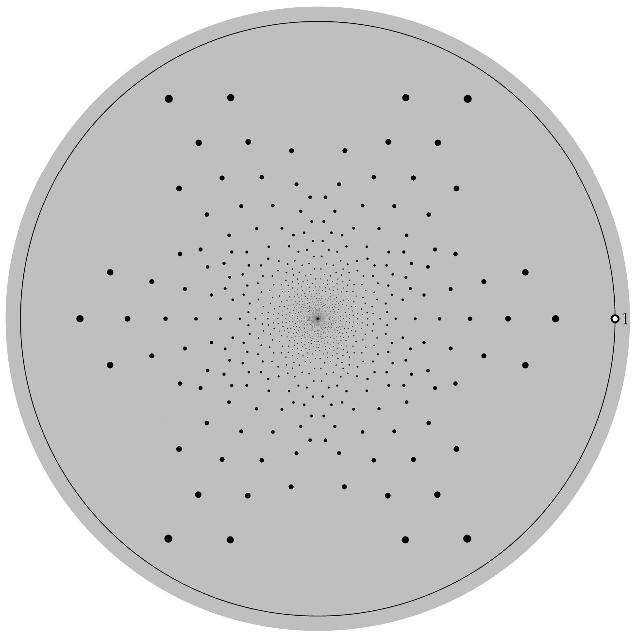
Figure 3: A plot of the spectrum of $\mathcal{C}_{T_{\lambda}}$, for $\lambda=0.8e^{31i\pi/50}$.

3.1 The Hilbert space $\mathcal{H}_{a,\phi}$

The space $\mathcal{H}_{a,\phi}$ is defined analogously to $\mathcal{H}_{a}$. The weights here, $\|e_{m,n}\|_{a,\phi},$ depend on the following simple generalisation, $\deg_{\phi}$, of $\deg_{1}$.

Definition 3.3 ($\deg_{\phi}$, $\|\cdot\|_{a,\phi}$, $\mathcal{H}_{a,\phi}$).

For $\phi>1$, let

$$\deg_{\phi}(m,n):=\deg_{1}(m,\phi^{-\operatorname{sign}(m,n)}n)=\begin{cases}\phantom{-}|m|+\phi^{-1}|n|&\text{if }mn\geq 0;\\ -|m|-\phi^{\phantom{-1}}|n|&\text{if }mn<0.\end{cases}$$

For $a>0$, we write

$$\|e_{m,n}\|_{a,\phi}:=e^{-a\deg_{\phi}(m,n)}.$$

As before, this norm extends to arbitrary linear combinations of the $e_{m,n}$:

$$\bigg{\|}\sum_{m,n}b_{m,n}e_{m,n}\bigg{\|}_{a,\phi}^{2}=\sum_{m,n}|b_{m,n}|^{2}e^{-2a\deg_{\phi}(m,n)},$$

The following result shows that, as for $\mathcal{H}_{a}$, the Hilbert space $\mathcal{H}_{a,\phi}$ can be chosen to contain analytic functions on a neighbourhood of the torus.

Proposition 3.4.

For $a>0$ and $\phi>1$, suppose that $f$ is an analytic function on a neighbourhood of the poly-annulus

$$P_{a,\phi}:=\{(z,w)\in\mathbb{C}^{2}\;|\;e^{-a}\leq|z|\leq e^{a},\ e^{-a\phi}\leq|w|\leq e^{a\phi}\}.$$

Then $f\in\mathcal{H}_{a,\phi}$. In particular, every function analytic on a neighbourhood of $\mathbb{T}^{2}$ is contained in $\mathcal{H}_{a,\phi}$, for all $(a,\phi)$ such that $a\phi$ is sufficiently small.

Proof.

The proof is very similar to that of Proposition 2.6. Fix $a$, $\phi$ and $f$ as above. By construction, the expansion

$$f(z,w)=\sum_{(m,n)\in\mathbb{Z}^{2}}b_{m,n}\,z^{m}w^{n}$$ (16)

converges absolutely for all $(z,w)\in P_{a,\phi}$. Also, one has the following bound from the definition of $\|f\|_{a,\phi}$, using that $-\deg_{\phi}(m,n)\leq|m|+\phi|n|$:

$$\|f\|_{a,\phi}^{2}:=\sum_{(m,n)\in\mathbb{Z}^{2}}|b_{m,n}|^{2}\,e^{-2a\deg_{\phi}(m,n)}\leq\sum_{(m,n)\in\mathbb{Z}^{2}}|b_{m,n}|^{2}\,e^{2a(|m|+\phi|n|)}.$$ (17)

Considering the right hand side, one bounds a related sum

$$\sum_{(m,n)\in\mathbb{Z}^{2})}|b_{m,n}|\,e^{a(|m|+\phi|n|)} \leq\sum_{(m,n)\in\mathbb{Z}^{2})}|b_{m,n}|e^{a(m+\phi n)}+\sum_{(m,n)\in\mathbb{Z}^{2})}|b_{m,n}|e^{a(m-\phi n)}$$

$$\phantom{{}\leq{}}+\sum_{(m,n)\in\mathbb{Z}^{2})}|b_{m,n}|e^{a(-m-\phi n)}+\sum_{(m,n)\in\mathbb{Z}^{2})}|b_{m,n}|e^{a(-m+\phi n)},$$

each of which is convergent by the absolute convergence of (16) for all $(z,w)\in\{(e^{\pm a},e^{\pm a\phi})\}\subset P_{a,\phi}$. In particular, the sum on the left is square-summable, i.e., the sum on the right hand side of (17) is finite. Thus, $f\in\mathcal{H}_{a,\phi}$ as required. ∎

3.2 $\mathcal{C}_{T_{\lambda}}$ is Hilbert-Schmidt

To begin the proof of Theorem 3.2 we now give the following compactness result. Note that, fixing $a$ and $\lambda$, its hypothesis is satisfied for all $\phi$ sufficiently close to 1.

Proposition 3.5.

Given $\lambda$ with $|\lambda|<1$, $a>0$ and $\phi>1$, if

$$2a(\phi-1)<-\log M_{a,\lambda},$$

the composition operator $\mathcal{C}_{T_{\lambda}}:\mathcal{H}_{a,\phi}\to\mathcal{H}_{a,\phi}$ is Hilbert-Schmidt.

The proof of this proposition is similar to that of Proposition 2.10.

Proof.

Formally expanding

$$e_{m,n}\big{(}T_{\lambda}(z,w)\big{)}=w^{m}\left({\frac{z+w}{1+\overline{w}z}}\right)^{m}z^{n}$$

gives the following, for $\sigma=\hbox{\rm sign}(m)$:

$$\mathcal{C}_{T_{\lambda}}(e_{m,n})=\begin{cases}\displaystyle\sum_{k=0}^{\infty}\alpha_{m,k}\,e_{n+\sigma k,m},&m\neq 0;\\ \qquad e_{n,m},&m=0.\end{cases}$$ (18)

In particular, for $m\neq 0$,

$$\left(\frac{\|\mathcal{C}_{T_{\lambda}}(e_{m,n})\|_{a,\phi}}{\|e_{m,n}\|_{a,\phi}}\right)^{2} =\sum_{k=0}^{\infty}|\alpha_{m,k}|^{2}\left(\frac{\|e_{n+\sigma k,m}\|_{a,\phi}}{\|e_{m,n}\|_{a,\phi}}\right)^{2}$$

$$=\sum_{k=0}^{\infty}|\alpha_{m,k}|^{2}e^{2a\big{(}\deg_{\phi}(m,n)-\deg_{\phi}(n+\sigma k,m)\big{)}}$$

$$=e^{2a\big{(}\deg_{\phi}(m,n)-\deg_{\phi}(n,m)\big{)}}\sum_{k=0}^{\infty}|\alpha_{m,k}|^{2}e^{2a\big{(}\deg_{\phi}(n,m)-\deg_{\phi}(n+\sigma k,m)\big{)}}.$$

Considering first the prefactor, we find that

$$I(m,n):=\deg_{\phi}(m,n)-\deg_{\phi}(n,m) =\begin{cases}\phi^{-1}(\phi-1)\big{(}|m|-|n|\big{)},&\text{if }mn\geq 0;\\ \phantom{\phi}{}^{\phantom{-1}}(\phi-1)\big{(}|m|-|n|\big{)},&\text{if }mn<0.\end{cases}$$

Also, as in the proof of Lemma 2.11, considering three cases for $\deg_{\phi}(n+\sigma,m)-\deg_{\phi}(n,m)$, we find that

$$\deg_{\phi}(n+\sigma,m)-\deg_{\phi}(n,m) =\begin{cases}2|n|+\phi^{-1}+\phi-1,&\text{if }mn<0\text{ and }|m|=1;\\ 1,&\text{otherwise}.\end{cases}$$

$$\geq\rule{9.45pt}{0.0pt}1.$$

Therefore by induction, $\deg_{\phi}(n+\sigma k,m)-\deg_{\phi}(n,m)\geq k$ for all $k\in\mathbb{N}$. Thus, for all $(m,n)\in\left(\mathbb{Z}\backslash\{0\}\right)\times\mathbb{Z}$ (applying Lemma 2.8),

$$\left(\frac{\|\mathcal{C}_{T_{\lambda}}(e_{m,n})\|_{a,\phi}}{\|e_{m,n}\|_{a,\phi}}\right)^{2} \leq e^{2aI(m,n)}\sum_{k=0}^{\infty}|\alpha_{m,k}|^{2}e^{-2ak}.$$

$$\leq e^{2aI(m,n)}M_{a,\lambda}^{|m|}$$

$$=\begin{cases}e^{2a\phi^{-1}(\phi-1)\big{(}|m|-|n|\big{)}}M^{|m|}_{a,\lambda},&\text{if }mn\geq 0;\\ \hphantom{\vphantom{e}{}^{\phi^{-1}}}e^{2a(\phi-1)\big{(}|m|-|n|\big{)}}M^{|m|}_{a,\lambda},&\text{if }mn<0.\end{cases}$$

Considering the exponents on the right hand side, if

$$2a(\phi-1)=2a\max\big{(}\phi-1,\phi^{-1}(\phi-1)\big{)}<-\log(M_{a,\lambda}),$$

then $\delta:=\min\big{(}2a\phi^{-1}(\phi-1),2a(1-\phi)-\log(M_{a,\lambda})\big{)}$ is positive and satisfies

$$\left(\frac{\|\mathcal{C}_{T_{\lambda}}(e_{m,n})\|_{a,\phi}}{\|e_{m,n}\|_{a,\phi}}\right)^{2}\leq e^{-\delta\big{(}|m|+|n|\big{)}}$$

whenever $m\neq 0$. This inequality also applies in the $m=0$ case:

$$\left(\frac{\|\mathcal{C}_{T_{\lambda}}(e_{0,n})\|_{a,\phi}}{\|e_{0,n}\|_{a,\phi}}\right)^{2}=\left(\frac{\|e_{n,0}\|_{a,\phi}}{\|e_{0,n}\|_{a,\phi}}\right)^{2}=e^{-2aI(0,n)}\leq e^{-2a\phi^{-1}(\phi-1)|n|}\leq e^{-\delta|n|}.$$

Thus,

$$\|\mathcal{C}_{T_{\lambda}}\|_{\text{HS}}^{2}=\sum_{(m,n)\in\mathbb{Z}^{2}}\left(\frac{\|\mathcal{C}_{T_{\lambda}}(e_{m,n})\|_{a,\phi}}{\|e_{m,n}\|_{a,\phi}}\right)^{2}\leq\sum_{(m,n)\in\mathbb{Z}^{2}}e^{-\delta(|m|+|n|)}<\infty,$$

i.e., $\mathcal{C}_{T_{\lambda}}$ is Hilbert-Schmidt, as required. ∎

Remark 3.6.

In fact, $a(\phi-1)$ being small is necessary for $\mathcal{C}_{T_{\lambda}}$ on $\mathcal{H}_{a,\phi}$ to be bounded, let alone compact: For example, let $m>0$, $n<0$. Then, considering the first term of the expansion (18) gives

$$\frac{\|\mathcal{C}_{T_{\lambda}}(e_{m,n})\|_{a,\phi}}{\|e_{m,n}\|_{a,\phi}}\geq|\lambda|^{m}\frac{\|e_{n,m}\|_{a,\phi}}{\|e_{m,n}\|_{a,\phi}}=|\lambda|^{m}e^{aI(m,n)}=|\lambda|^{m}e^{a(\phi-1)(m+n)}.$$

Thus, if $-\log|\lambda|<a(\phi-1)$, the right hand side can be made arbitrarily large.

3.3 The spectrum of $\mathcal{C}_{T_{\lambda}}$

The following concludes the proof of Theorem 3.2.

Lemma 3.7.

For $\lambda$, $a$ and $\phi$ as in Proposition 3.4, the spectrum of $\mathcal{C}_{T_{\lambda}}:\mathcal{H}_{a,\phi}\to\mathcal{H}_{a,\phi}$ is as follows, where $\lambda_{1}$ is a square root of $\lambda$:

$$\{0,1\}\cup\big{\{}\omega\lambda_{1}^{m}\overline{\lambda}_{1}^{n}\mid\omega=\pm 1,\ (m,n)\in\mathbb{N}_{0}^{2}\setminus\{(0,0)\}\big{\}}.$$

Each non-zero eigenvalue is semi-simple. Up to coincidences in value, the eigenvalues $\omega\lambda_{1}^{k}$, $\omega\overline{\lambda}_{1}^{k}$ have multiplicity

$$N(k,\omega)=\begin{cases}\left\lfloor\frac{k}{2}\right\rfloor+1,&\text{if }\omega=\phantom{-}1;\\ \left\lfloor\frac{k+1}{2}\right\rfloor,&\text{if }\omega=-1;\end{cases}$$

and all other non-zero eigenvalues are simple.

Proof.

The proof of this result is analogous to the proof of Proposition 2.10. Recalling that $\alpha_{m,0}=\lambda^{m}$ for $m\in\mathbb{N}$, the expansion for $\mathcal{C}_{T_{\lambda}}(e_{m,n})$ reads

$$\mathcal{C}_{T_{\lambda}}(e_{m,n})=\begin{cases}\displaystyle\lambda^{m\hphantom{||}}e_{n,m}+\sum_{k=1}^{\infty}\alpha_{m,k}\,e_{n+k,m},&\text{if }m>0;\\ \hphantom{\lambda^{|m|}}e_{n,m},&\text{if }m=0;\\ \rule{0.0pt}{20.0pt}\displaystyle\overline{\lambda}\vphantom{\lambda}^{|m|}e_{n,m}+\sum_{k=1}^{\infty}\alpha_{m,k}\,e_{n-k,m},&\text{if }m<0.\end{cases}$$

By Lemma 2.11, for any $m\neq 0$ and $k\in\mathbb{N}$,

$$\deg_{1}(m,n)=\deg_{1}(n,m)<\deg_{1}\big{(}n+\operatorname{sign}(m)k,m\big{)}.$$

Since the first equality applies for $m=0$ also, this shows that $\mathcal{C}_{T_{\lambda}}$ increases $\deg_{1}$, and that the corresponding $\big{(}\mathcal{C}_{T_{\lambda}}\big{)}_{k}(e_{m,n})$ is obtained by eliminating the sums above: that is,

$$\big{(}\mathcal{C}_{T_{\lambda}}\big{)}_{k}=\Pi_{D_{k}}\circ\mathcal{C}_{T_{\lambda}}\circ\Pi_{D_{k}}:e_{m,n}\mapsto\begin{cases}\lambda^{m}e_{n,m},&\text{if }m\geq 0,\ \deg_{1}(m,n)=k;\\ \overline{\lambda}^{|m|}e_{n,m},&\text{if }m<0,\ \deg_{1}(m,n)=k;\\ 0,&\text{otherwise;}\end{cases}$$

where $D_{k}:=\operatorname{Span}\{e_{m,n}\,|\,\deg_{1}(m,n)=k\}$ is as before. Thus, pairing up $e_{m,n}$ and $e_{n,m}$ for $m\neq n$, one has the following block-diagonal matrix representation of $\big{(}\mathcal{C}_{T_{\lambda}}\big{)}_{k}$, depending on $k$:

$$\big{(}\mathcal{C}_{T_{\lambda}}\big{)}_{k}\cong\begin{cases}\hphantom{\rule{0.0pt}{25.0pt}\displaystyle\bigoplus_{n=0}^{(n-2)/2}}\qquad\big{(}\,1\,\big{)},&k=0;\\ \rule{0.0pt}{25.0pt}\displaystyle\bigoplus_{n=0}^{(k-2)/2}\begin{pmatrix}0&\lambda^{n}\\ \lambda^{k-n}&0\end{pmatrix}\oplus\begin{pmatrix}0&\overline{\lambda}{\vphantom{\lambda}}^{n}\\ \overline{\lambda}{\vphantom{\lambda}}^{k-n}&0\end{pmatrix}\ \oplus\;\big{(}\lambda^{k/2}\big{)}\oplus\big{(}\overline{\lambda}{\vphantom{\lambda}}^{k/2}\big{)},&k\in 2\mathbb{N};\\ \rule{0.0pt}{25.0pt}\displaystyle\bigoplus_{n=1}^{(k-1)/2}\begin{pmatrix}0&\lambda^{n}\\ \lambda^{k-n}&0\end{pmatrix}\oplus\begin{pmatrix}0&\overline{\lambda}{\vphantom{\lambda}}^{n}\\ \overline{\lambda}{\vphantom{\lambda}}^{k-n}&0\end{pmatrix},&k\in 2\mathbb{N}-1;\\ \rule{0.0pt}{25.0pt}\displaystyle\bigoplus_{\begin{subarray}{c}n=1\\ \hphantom{(k-1)/2}\end{subarray}}^{k-1}\begin{pmatrix}0&\lambda^{n}\\ \overline{\lambda}{\vphantom{\lambda}}^{k-n}&0\end{pmatrix},&k<0.\end{cases}$$

Applying Lemma 2.13 and counting multiplicities, the non-zero eigenvalues of $\mathcal{C}_{T_{\lambda}}$ and their multiplicities are precisely those given in the statement of the lemma. In particular, each non-zero eigenvalue is semi-simple, since the $\big{(}\mathcal{C}_{T_{\lambda}}\big{)}_{k}$ are diagonalisable and do not share eigenvalues when $\lambda$ is non-zero. ∎

4 The spectrum of $\mathcal{C}_{T_{\lambda}\circ T_{\mu}}$

Now that we have established the machinery for $T_{\lambda}$, the following result for $T_{\lambda}\circ T_{\mu}$ (with $|\lambda|,|\mu|<1$) will be very easy to prove. Again, we note that this family of examples appears in an appendix of [23], where their resonances are announced and numerically studied. We now provide a rigorous argument.

Theorem 4.1.

For $\lambda,\mu$ with $|\lambda|,|\mu|<1$ and $\mathcal{H}_{a,\phi}$ defined as above, if $a>0$ and $\phi>1$ satisfy

$$2a(\phi-1)<-\log\big{(}\max(M_{a,\lambda},M_{a,\mu})\big{)},$$ (19)

then $\mathcal{C}_{T_{\lambda}\circ T_{\mu}}=\mathcal{C}_{T_{\mu}}\circ\mathcal{C}_{T_{\lambda}}$ acts compactly on $\mathcal{H}_{a,\phi}$ and has spectrum

$$\{0,1\}\cup\big{\{}\lambda^{m}\mu^{n},\ \lambda^{m}\overline{\mu}\vphantom{\mu}^{n},\ \overline{\lambda}^{m}\overline{\mu}\vphantom{\mu}^{n},\ \overline{\lambda}^{m}\mu^{n}\mid(m,n)\in\mathbb{N}_{0}^{2}\setminus\{(0,0)\}\big{\}}.$$

Moreover, all non-zero eigenvalues are simple, up to coincidences in value.

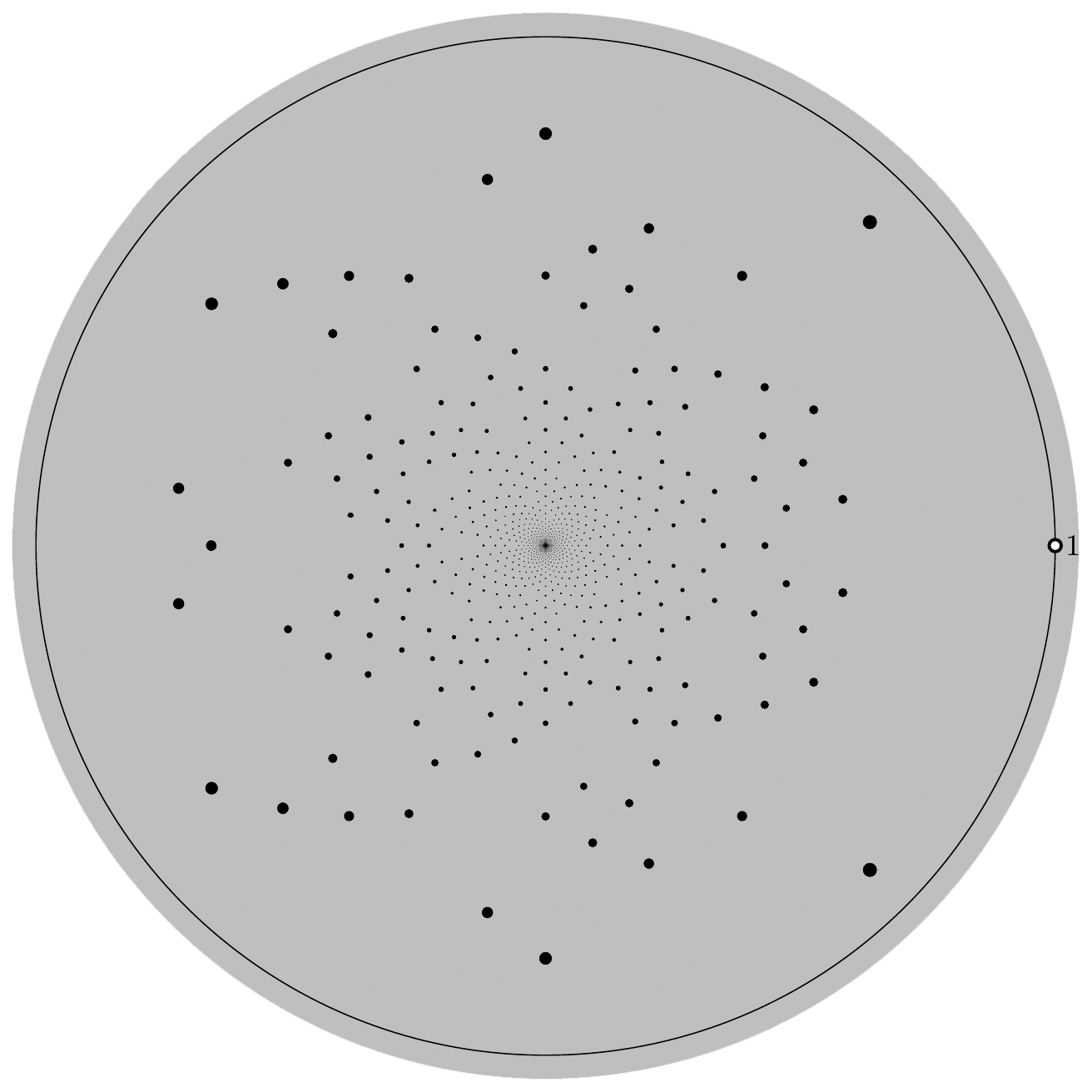
Figure 4: The spectrum of $\mathcal{C}_{T_{\lambda}\circ T_{\mu}}$, for $\lambda=0.9e^{i\pi/4}$, $\mu=0.65e^{6i\pi/5}$.

4.1 $\mathcal{C}_{T_{\lambda}\circ T_{\mu}}$ is trace-class

To begin the proof of Theorem 4.1 one has the following, simple corollary of Proposition 3.5.

We first recall [9, p.267] that being trace-class is a stronger property than being Hilbert-Schmidt, and that an operator is trace-class if and only if it is the composition of two Hilbert-Schmidt operators.

Lemma 4.2.

For $\lambda,\mu,a,\phi$ as in Theorem 4.1 the operator $\mathcal{C}_{T_{\lambda}\circ T_{\mu}}:\mathcal{H}_{a,\phi}\to\mathcal{H}_{a,\phi}$ is trace-class.

Remark 4.3.

Since $B_{\lambda}=T_{0}\circ T_{\lambda}$ for all $\lambda$, this shows that $\mathcal{C}_{B_{\lambda}}$ is trace-class as an operator on $\mathcal{H}_{a,\phi}$.

Proof.

By the hypothesis (19) Proposition 3.5 applies twice to show that $\mathcal{C}_{T_{\lambda}}$ and $\mathcal{C}_{T_{\mu}}$ are each Hilbert-Schmidt on $\mathcal{H}_{a,\phi}$. Thus $\mathcal{C}_{T_{\lambda}\circ T_{\mu}}=\mathcal{C}_{T_{\mu}}\circ\mathcal{C}_{T_{\lambda}}$ is the composition of two Hilbert-Schmidt operators, hence trace-class. ∎

4.2 The spectrum of $\mathcal{C}_{T_{\lambda}}\circ\mathcal{C}_{T_{\mu}}$

The calculation of the spectrum likewise follows simply from that of the previous section. This uses the following lemma, which naturally extends the corresponding intuitive result for block-triangular matrices in finite dimensions:

$$\begin{pmatrix}A_{1}&0&0&\cdots&0\\ \ast&A_{2}&0&\cdots&0\\ \ast&\ast&A_{3}&\cdots&0\\ \vdots&\vdots&\vdots&\ddots&\vdots\\ \ast&\ast&\ast&\cdots&A_{n}\\ \end{pmatrix}\begin{pmatrix}B_{1}&0&0&\cdots&0\\ \ast&B_{2}&0&\cdots&0\\ \ast&\ast&B_{3}&\cdots&0\\ \vdots&\vdots&\vdots&\ddots&\vdots\\ \ast&\ast&\ast&\cdots&B_{n}\\ \end{pmatrix}=\begin{pmatrix}A_{1}B_{1}&0&0&\cdots&0\\ \ast&A_{2}B_{2}&0&\cdots&0\\ \ast&\ast&A_{3}B_{3}&\cdots&0\\ \vdots&\vdots&\vdots&\ddots&\vdots\\ \ast&\ast&\ast&\cdots&A_{n}B_{n}\\ \end{pmatrix},$$

where $A_{k}$ and $B_{k}$ are square matrices of the same size for each $k$.

The proof of the lemma, like that of Lemma 2.13, is a simple extension of the finite case and we omit it (see [20]).

Lemma 4.4.

Let $\mathcal{H}$ be a Hilbert space such that $\{e_{m,n}\}_{(m,n)\in\mathbb{Z}^{2}}$ is an orthogonal basis, and let $\mathcal{C}_{1},\mathcal{C}_{2}:\mathcal{H}\to\mathcal{H}$ increase $\deg_{1}$. Then $\mathcal{C}_{1}\circ\mathcal{C}_{2}$ increases $\deg_{1}$ and satisfies, for each $k$,

$$\big{(}\mathcal{C}_{1}\circ\mathcal{C}_{2}\big{)}_{k}=\big{(}\mathcal{C}_{1}\big{)}_{k}\circ\big{(}\mathcal{C}_{2}\big{)}_{k}.$$ (20)

We now apply this lemma to give the resonances of $T_{\lambda}\circ T_{\mu}$.

Lemma 4.5.

For each $\lambda,\mu$, the spectrum of $\mathcal{C}_{T_{\lambda}\circ T_{\mu}}$ is given by

$$\{0,1\}\cup\big{\{}\lambda^{m}\mu^{n},\ \lambda^{m}\overline{\mu}\vphantom{\mu}^{n},\ \overline{\lambda}^{m}\overline{\mu}\vphantom{\mu}^{n},\ \overline{\lambda}^{m}\mu^{n}\mid(m,n)\in\mathbb{N}_{0}^{2}\setminus\{(0,0)\}\big{\}}.$$ (21)

Moreover, each non-zero eigenvalue has algebraic multiplicity equal to the frequency with which it appears in (21).

Proof.

Applying Lemmas 4.4 and 2.3 reduces the proof to a consideration of the eigenvalues of $\big{(}\mathcal{C}_{T_{\lambda}\circ T_{\mu}}\big{)}_{k}=\big{(}\mathcal{C}_{T_{\lambda}}\big{)}_{k}\circ\big{(}\mathcal{C}_{T_{\mu}}\big{)}_{k}.$ We recall from the proof of Lemma 3.7 that, for $k=\deg_{1}(m,n)$,

$$\big{(}\mathcal{C}_{T_{\mu}}\big{)}_{k}(e_{m,n})=\Pi_{D_{k}}\circ\mathcal{C}_{T_{\mu}}(e_{m,n})=\begin{cases}\mu^{m\phantom{||}}e_{n,m},&\text{if }m\geq 0;\\ \overline{\mu}^{|m|}e_{n,m},&\text{if }m<0.\end{cases}$$

Thus, for $k=\deg_{1}(m,n)=\deg_{1}(n,m)$,

$$\big{(}\mathcal{C}_{T_{\lambda}\circ T_{\mu}}\big{)}_{k}(e_{m,n})=\begin{cases}\mu^{m\phantom{||}}\lambda^{n\phantom{||}}e_{m,n},&\text{if }m\geq 0,\ n\geq 0;\\ \overline{\mu}^{|m|}\lambda^{n\phantom{||}}e_{m,n},&\text{if }m<0,\ n\geq 0;\\ \mu^{m\phantom{||}}\overline{\lambda}^{|n|}e_{m,n},&\text{if }m\geq 0,\ n<0;\\ \overline{\mu}^{|m|}\overline{\lambda}^{|n|}e_{m,n},&\text{if }m<0,\ n<0.\end{cases}$$

That is, each $\big{(}\mathcal{C}_{T_{\lambda}\circ T_{\mu}}\big{)}_{k}$ is diagonal. Since the prefactor of $e_{m,n}$ is unique (up to coincidences in value), this shows that the spectrum is given by

$$\{0,1\}\cup\big{\{}\lambda^{m}\mu^{n},\ \lambda^{m}\overline{\mu}\vphantom{\mu}^{n},\ \overline{\lambda}^{m}\overline{\mu}\vphantom{\mu}^{n},\ \overline{\lambda}^{m}\mu^{n}\mid(m,n)\in\mathbb{N}_{0}^{2}\setminus\{(0,0)\}\big{\}},$$

and that the non-zero eigenvalues are simple, up to coincidences in value (e.g. if $\lambda$, $\mu$ and $\mu/\lambda$ are non-zero and have arguments which are irrational multiples of $\pi$). ∎

This completes the proof of Theorem 4.1.

5 Final comments

1. The methods of §2 naturally extend to the following families of diffeomorphisms $B_{\lambda,K}:\mathbb{T}^{2}\to\mathbb{T}^{2}$ indexed by $K\in\mathbb{N}$ and $\lambda$ with $|\lambda|<1$:

$$B_{\lambda,K}:(z,w)\mapsto\left(\left(\frac{z+\lambda}{1+\overline{\lambda}z}\right)^{K^{2}+1}w^{K},\left(\frac{z+\lambda}{1+\overline{\lambda}z}\right)^{K}w\right),$$

which can be considered, for each $K$, as a perturbation of the hyperbolic linear automorphism given by (on $\mathbb{T}^{2}$ or $\mathbb{R}^{2}/\mathbb{Z}^{2}$ respectively)

$$B_{0,K}:(z,w)\mapsto\big{(}z^{K^{2}}zw^{K},\,z^{K}w\big{)}\qquad\text{or}\qquad\left(\begin{matrix}x\\ y\end{matrix}\right)\mapsto\begin{pmatrix}K^{2}&\!\!K\\ K^{\phantom{2}}&\!\!1\end{pmatrix}\left(\begin{matrix}x\\ y\end{matrix}\right)\mod 1.$$

However, since the resonances of $B_{\lambda,K}$ equal those of $B_{\lambda^{K}}$, these families contribute nothing new to the variety of spectra presented here.

2. In §3 one could again extend the analysis to related families of examples: i.e., for $K\in\mathbb{N}$ and $|\lambda|<1$, consider

$$T_{\lambda,K}:(z,w)\mapsto\left(\left(\frac{z+\lambda}{1+\overline{\lambda}z}\right)^{K}w,z\right),$$

perturbing, for each $K$, the hyperbolic linear automorphism

$$T_{0,K}:(z,w)\mapsto(z^{K}w,z)\qquad\longleftrightarrow\qquad\left(\begin{matrix}x\\ y\end{matrix}\right)\mapsto\begin{pmatrix}K&1\\ 1&0\end{pmatrix}\left(\begin{matrix}x\\ y\end{matrix}\right),$$

the orientation-reversing square root of $B_{0,K}$. However again, we would find that that the spectrum of $T_{\lambda,K}$ equals that of $T_{\lambda^{K}}$, so these families contribute nothing extra in variety.

3. To see why we introduced $\mathcal{H}_{a,\phi}$ in §3, we exhibit the following negative result, which shows that $\mathcal{C}_{T_{\lambda}}$ does not act compactly on either $\mathcal{H}_{a}$ or the anisotropic space used in [23], for any non-zero $\lambda$.

Proposition 5.1.

Suppose that $\mathcal{H}$ is a Hilbert space which has $\{e_{m,n}\}_{m,n}$ as an orthogonal basis, and satisfies, for all $(m,n)\in\mathbb{Z}^{2}$,

$$\|e_{m,n}\|=\|e_{n,m}\|.$$

Then, $\mathcal{C}_{T_{\lambda}}$ is not compact on $\mathcal{H}$, for any $\lambda\neq 0$.

Proof.

Fix $m\in\mathbb{N}$ and $\lambda$. Then, recalling (18), we have

$$\mathcal{C}_{T_{\lambda}}(e_{m,n})=\lambda^{m}e_{n,m}+\sum_{k=1}^{\infty}\alpha_{m,k}e_{n+k,m},$$

and thus, by orthogonality,

$$\|\mathcal{C}_{T_{\lambda}}(e_{m,n})\|^{2}\geq|\lambda|^{2m}\|e_{m,n}\|^{2}.$$ (22)

If $\mathcal{C}_{T_{\lambda}}$ is compact, it maps the sequence $(e_{m,n}/\|e_{m,n}\|)_{n=1}^{\infty}$, which weakly converges to zero, onto one which converges to zero in $\mathcal{H}$. But this contradicts (22), so it is not compact. ∎

References

-
[1]
A. Adam.
Generic non-trivial resonances for Anosov diffeomorphisms.
Nonlinearity 30 (2017), no. 3, 1146–64.
doi:10.1088/1361-6544/aa59a9 - [2] V. I. Arnold and A. Avez. Problèmes ergodiques de la mécanique classique. Gauthier-Villars: Paris, 1967.
- [3] V. Baladi. Dynamical zeta functions and dynamical determinants for hyperbolic maps: A functional approach. A Series of Modern Surveys in Mathematics, 3rd Series, 68. Springer: Cham, 2018. ISBN:978-3-319-77660-6
-
[4]
V. Baladi.
The quest for the ultimate anisotropic Banach space.
J. Stat. Phys. 166 (2017), no. 3–4, 525–557.
doi:10.1007/s10955-016-1663-0 -
[5]
O. Bandtlow and O. Jenkinson. On the Ruelle eigenvalue sequence.
Ergodic Theory and Dynam. Systems 28 (2008), no. 6, 1701–1711.
doi:10.1017/S0143385708000059 -
[6]
O. Bandtlow, W. Just and J. Slipantschuk.
Spectral structure of transfer operators for expanding circle maps.
Ann. Inst. H. Poincaré Anal. Non Linéaire 34 (2017), no. 1, 31–43.
doi:10.1016/j.anihpc.2015.08.004 -
[7]
O. Bandtlow and F. Naud.
Lower bounds for the Ruelle spectrum of analytic expanding circle maps.
Ergodic Theory Dynam. Systems 39 (2019), no. 2, 289–310.
doi:10.1017/etds.2017.29 -
[8]
E. G. D. Cohen and G. Gallavotti.
Dynamical Ensembles in Nonequilibrium Statistical Mechanics.
Phys. Rev. Lett. 74 (1995), 2694–2697.
doi:10.1103/PhysRevLett.74.2694 -
[9]
J. B. Conway.
A course in functional analysis.
Second edition. Graduate Texts in Math. 96.
Springer-Verlag: New York, 1990.
doi:10.1007/978-1-4757-4383-8 -
[10]
C. C. Cowen.
Composition Operators on Spaces of Analytic Functions II.
Lecture notes: Spring School of Functional Analysis, Rabat, 19–21 May 2009.
math.iupui.edu/~ccowen/Talks/CompOp0905slidesB.pdf -
[11]
M. F. Demers.
A gentle introduction to anisotropic Banach spaces.
Chaos Solitons Fractals 116 (2018), 29–42.
doi:10.1016/j.chaos.2018.08.028 -
[12]
R. Durrett.
Probability: theory and examples.
Fifth edition. Cambridge Series in Statistical and Probabilistic Mathematics 49. Cambridge University Press: Cambridge, 2019.
doi:10.1017/9781108591034 - [13] B. Farb and D. Margalit. A primer on mapping class groups. Princeton Mathematical Series, 49. Princeton University Press: Princeton, 2012. ISBN:978-0-691-14794-9
-
[14]
F. Faure and N. Roy.
Ruelle-Pollicott resonances for real analytic hyperbolic maps.
Nonlinearity 19 (2006), no. 6, 1233–1252.
doi:10.1088/0951-7715/19/6/002 -
[15]
F. Faure, S. Gouëzel and E. Lanneau.
Ruelle spectrum of linear pseudo-Anosov maps.
J. Éc. polytech. Math. 6 (2019), 811–877.
doi:10.5802/jep.107 -
[16]
F. Naud.
The Ruelle spectrum of generic transfer operators.
Discrete Contin. Dynam. Systems 32 (2012), no. 7, 2521–2531.
doi:10.3934/dcds.2012.32.2521 - [17] E. R. Pujals and R. K. W. Roeder. Two-dimensional Blaschke products: degree growth and ergodic consequences. Indiana Univ. Math. J. 59 (2010), no. 1, 301–325.
-
[18]
E. R. Pujals and M. Shub.
Dynamics of two-dimensional Blaschke products.
Ergodic Theory Dynam. Systems 28 (2008), no. 2, 575–85.
doi:10.1017/S0143385707000752 - [19] W. Rudin. Functional analysis. Second edition. International Series in Pure and Applied Mathematics. McGraw-Hill: New York, 1991. ISBN:0-07-054236-8
-
[20]
B. Sewell.
Equidistribution of infinite interval substitution schemes, explicit resonances of Anosov toral maps, and the Hausdorff dimension of the Rauzy gasket. PhD thesis. Available from
www.warwick.ac.uk/fac/sci/maths/people/staff/sewell - [21] J. H. Shapiro. Composition operators and classical function theory. Universitext: Tracts in Mathematics. Springer-Verlag: New York, 1993. ISBN:0-387-94067-7
-
[22]
J. Slipantschuk, O. Bandtlow and W. Just.
Analytic expanding circle maps with explicit spectra.
Nonlinearity 26 (2013), no. 12, 3231–45.
doi:10.1088/0951-7715/26/12/3231 -
[23]
J. Slipantschuk, O. Bandtlow and W. Just.
Complete spectral data for analytic Anosov maps of the torus.
Nonlinearity 30 (2017), no. 7, 2667–86.
doi:10.1088/1361-6544/aa700f -
[24]
T. J. Sullivan.
Introduction to uncertainty quantification.
Texts in Applied Mathematics 63. Springer: Cham, 2015.
doi:10.1007/978-3-319-23395-6 -
[25]
L.-S. Young.
What are SRB measures, and which dynamical systems have them?
J. Stat. Phys. 108 (2002), no. 5-6, 733–754.
doi:10.1023/A:1019762724717