Degradation-agnostic Correspondence from Resolution-asymmetric Stereo

Abstract

In this paper, we study the problem of stereo matching from a pair of images with different resolutions, e.g., those acquired with a tele-wide camera system. Due to the difficulty of obtaining ground-truth disparity labels in diverse real-world systems, we start from an unsupervised learning perspective. However, resolution asymmetry caused by unknown degradations between two views hinders the effectiveness of the generally assumed photometric consistency. To overcome this challenge, we propose to impose the consistency between two views in a feature space instead of the image space, named feature-metric consistency. Interestingly, we find that, although a stereo matching network trained with the photometric loss is not optimal, its feature extractor can produce degradation-agnostic and matching-specific features. These features can then be utilized to formulate a feature-metric loss to avoid the photometric inconsistency. Moreover, we introduce a self-boosting strategy to optimize the feature extractor progressively, which further strengthens the feature-metric consistency. Experiments on both simulated datasets with various degradations and a self-collected real-world dataset validate the superior performance of the proposed method over existing solutions.

1 Introduction

Tele-wide camera systems consisting of two (or more) lenses with different focal lengths are widely deployed in smartphones nowadays. This kind of systems usually generates a pair (or a set) of images with different resolutions at one shot, which enables a number of desirable applications, such as continuous optical zoom [29] and image quality enhancement [37, 41, 43]. For these applications, correspondence estimation from resolution-asymmetric stereo images is a key step, which is typically conducted by conventional symmetric stereo matching algorithms (e.g., SGM [13]) together with image upsampling [29]. However, this straightforward solution is vulnerable to the artifacts introduced by upsampling, especially when the upsampling scale is large.

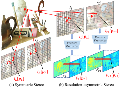
Figure 1: The common assumption of photometric consistency (i.e., $I_{L}[\textit{{p}}_{L}]$=$I_{R}[\textit{{p}}_{R}]$) in symmetric stereo is violated in resolution-asymmetric stereo (represented by dense and sparse grids). To avoid such photometric inconsistency (i.e., $I_{L}[\textit{{p}}_{L}]$$\neq$$I_{r\uparrow}[\textit{{p}}_{r\uparrow}]$), we establish the feature-metric consistency, which ensures that the pixels (e.g., $\textit{{p}}_{L}$ and $\textit{{p}}_{r\uparrow}$), recording the light rays (red arrows) emitted from the same scene point (e.g., P), have the same feature representation (i.e., $F_{L}[\textit{{p}}_{L}]$=$F_{r\uparrow}[\textit{{p}}_{r\uparrow}]$).

Asymmetric stereo matching has been studied in literature under several specific contexts, e.g., radiometric variation [15] and modality difference [49]. In this paper, we focus on the resolution-asymmetric setting, which is practical yet has rarely been investigated explicitly. As a recent related work, Liu et al. propose a unified network for visually imbalanced stereo matching that addresses monocular blur and noise [25]. Despite of its inspiring idea, this fully supervised approach requires not only the ground-truth disparity and the high-quality version of the degraded view as labels but also the explicit degradation [3, 7, 44, 17, 42] form to learn the parameters of the network, making it difficult to be applicable in diverse real-world systems where the supervision information is seldom available. Therefore, we turn to the direction of unsupervised learning.

For unsupervised stereo matching, the most widely adopted assumption is photometric consistency [50]. Under this assumption, the corresponding pixels in two views (e.g., $\textit{{p}}_{L}$ and $\textit{{p}}_{R}$ in Fig. 1(a)), which record the light rays emitted from the same scene point (e.g., P), should have the same intensity or color (i.e., $I_{L}[\textit{{p}}_{L}]$=$I_{R}[\textit{{p}}_{R}]$). Unfortunately, this assumption is violated for a resolution-asymmetric stereo pair, where the low-resolution (LR) view is degraded by an unknown downsampling kernel compared to the high-resolution (HR) view. In other words, the corresponding pixels in the asymmetric stereo pair (e.g., $\textit{{p}}_{L}$ and $\textit{{p}}_{r\uparrow}$ in Fig. 1(b)) may not have the same intensity or color (i.e., $I_{L}[\textit{{p}}_{L}]$$\neq$$I_{r\uparrow}[\textit{{p}}_{r\uparrow}]$). Such photometric inconsistency will result in difficulties for correspondence learning. A possible solution for remedy is to restore the LR view to an HR one by super-resolution (SR) techniques [10, 48, 26]. However, existing SR methods are mostly degradation-specific and suffer from performance drops if the real degradation is different from the assumed one (for non-blind SR) or not inside the assumed range (for blind SR) [6, 23, 47, 4]. Therefore, the effectiveness of SR methods to make up the photometric inconsistency will be hindered in practice.

To overcome the above challenge, we propose to solve resolution-asymmetric stereo matching from a new perspective by imposing the consistency of two views in a feature space instead of the image space, named feature-metric consistency. Interestingly, we find that, although a stereo matching network trained with the photometric loss is not optimal, its feature extractor can produce degradation-agnostic (i.e., robustness to the degradation between $I_{L}$ and $I_{r\uparrow}$) and matching-specific features for corresponding asymmetric pixels (i.e., $F_{L}[\textit{{p}}_{L}]$=$F_{r\uparrow}[\textit{{p}}_{r\uparrow}]$ in Fig. 1(b)). These features can then be utilized to formulate a feature-metric loss to avoid the photometric inconsistency. Moreover, by finetuning the stereo matching network using the feature-metric loss, we can optimize the feature extractor to capture more consistent properties from the stereo pair, strengthening the feature-metric consistency. To this end, we introduce a self-boosting strategy to optimize the feature extractor progressively. Specifically, we use the feature extractor learned from the previous stage to form a new feature-metric loss for the current stage. In this way, our method remains effective even for large degradations.

To quantitatively evaluate the performance of our method, we simulate four resolution-asymmetric stereo datasets, two from the widely used stereo datasets Middlebury [14] and KITTI2015 [28] and two from the light field datasets Inria_SLFD [32] and HCI [16] with a narrow baseline between two views which is closer to the configuration on smartphones. The LR view is generated under various degradations from its original HR version. To evaluate our method in real-world scenarios, we collect a resolution-asymmetric stereo dataset with the tele-wide camera system equipped on a Huawei P30 smartphone. Experimental results on both simulated and real-world datasets demonstrate that our method outperforms existing as well as potential solutions by a large margin.

Contributions of this paper are summarized as follows:

• The first unsupervised learning method for correspondence estimation from resolution-asymmetric stereo.

• An effective and efficient realization of feature-metric consistency to avoid photometric inconsistency caused by unknown degradations.

• A self-boosting strategy to strengthen feature-metric consistency by progressive loss update.

• Distinct performance improvements over comparison methods on both simulated and real-world datasets.

2 Related Work

Stereo Matching. Stereo matching, symmetric by default, has been extensively studied as a classical computer vision task for decades [31, 13]. Recently, deep learning based stereo matching methods have notably surpassed conventional algorithms. According to whether or not ground-truth disparity maps are required as labels, these methods can be divided into supervised [27, 18, 5, 8, 20] and unsupervised [50, 51, 39, 2] categories. In many real-world systems where the labels are not readily available, unsupervised methods enable learning without ground-truth information, most of which exploit the assumption of photometric consistency to formulate a photometric loss [50, 39, 36, 52, 9, 30]. However, this assumption will be violated when stereo images become asymmetric.

Asymmetric Stereo Matching. Several kinds of asymmetry have been considered in literature for stereo matching, including radiometric variation [15], modality difference [49], and visual quality imbalance [25]. To estimate correspondence from stereo images with radiometric variation, different robust matching costs are proposed, such as mutual information measure [11] and adaptive normalized cross-correlation [12]. For cross-modal stereo [49, 40, 45], images from two different modalities are normalized to a single one to make up the photometric inconsistency, e.g., through deep transformation networks [49, 21]. Recently, stereo matching with visual imbalance (monocular blur and noise) is addressed by integrating a view synthesis network and a stereo reconstruction network, which requires the ground-truth disparity, the high-quality version of the degraded view, and the explicit degradation form for supervision [25]. Resolution asymmetry can be regarded as a certain kind of visual imbalance, but such a supervised solution is difficult to be applicable in diverse real-world systems.

Feature-metric Learning. For geometry tasks, there are several pioneering works to utilize deep features as the metric of unsupervised learning. Specifically, Zhang et al. improve the performance of monocular depth estimation by integrating the photometric loss and a feature-metric loss based on pre-trained features [46]. Different from [46], Shu et al. learn customized features with an auto-encoder and two regularizing losses [34], while Spencer et al. learn features with the contrastive loss [35]. For domain adaptation, Liu et al. propose to penalize the matching error of a stereo network in the feature space of a domain translation network [24]. Inspired by the above works, for the first time, we introduce the concept of feature-metric consistency to the new task of resolution-asymmetric stereo matching.

3 Preliminary

A pair of resolution-asymmetric stereo images consists of an HR view and an LR view. Without loss of generality, we take the left view $I_{L}\in\mathbb{R}^{H\times W}$ as the HR view and the right view $I_{r}\in\mathbb{R}^{\frac{H}{s}\times\frac{W}{s}}$ as the LR view, where $s$ is an asymmetric factor. To align their resolutions, $I_{r}$ is upsampled with a classical interpolation algorithm (e.g., bicubic), denoted as $I_{r\uparrow}\in\mathbb{R}^{H\times W}$. Despite being upsampled, the high-frequency information in $I_{r\uparrow}$ is absent, and thus the stereo pair $I_{L}$ and $I_{r\uparrow}$ is still asymmetric.

3.1 Learning with Photometric Consistency

Given a stereo pair $I_{L}$ and $I_{r\uparrow}$ as input, an unsupervised stereo matching network $\Phi(\cdot;\theta)$ aims to predict a disparity map for $I_{L}$, denoted as $d_{L}=\Phi(I_{L},I_{r\uparrow};\theta)$, under the assumption of photometric consistency between the corresponding pixels in two views (denoted as $\textit{{p}}_{L}$ and $\textit{{p}}_{r\uparrow}$), i.e.,

$$I_{L}[\textit{{p}}_{L}]=I_{r\uparrow}[\textit{{p}}_{r\uparrow}].\vspace{-0.5mm}$$ (1)

If the disparity $d_{L}[\textit{{p}}_{L}]$ between $\textit{{p}}_{L}$ and $\textit{{p}}_{r\uparrow}$ is accurately estimated, $I_{L}[\textit{{p}}_{L}]$ in the left view can be well reconstructed by warping $I_{r\uparrow}[\textit{{p}}_{r\uparrow}]$ in the right view with this disparity as

$$I_{r\uparrow\rightarrow L}[\textit{{p}}_{L}]=I_{r\uparrow}[\textit{{p}}_{L}-d_{L}[\textit{{p}}_{L}]].\vspace{-1.25mm}$$ (2)

Therefore, the photometric loss is formulated as the reconstruction error between $I_{L}$ and its reconstructed version $I_{r\uparrow\rightarrow L}$, typically in the form of a weighted combination of $L_{1}$ and SSIM distance, i.e.,

$$\mathcal{L}_{pm}=\left\|I_{L}-I_{r\uparrow\rightarrow L}\right\|_{1}+\alpha(1-{\rm SSIM}(I_{L},I_{r\uparrow\rightarrow L})),\vspace{-1.25mm}$$ (3)

where $\alpha$ is a weighting factor.

3.2 Challenge and Motivation

Intuitively, resolution asymmetry challenges unsupervised stereo matching in twofold: (i) It may be more difficult for the feature extractor of the network to extract symmetric features from the asymmetric input, and (ii) the photometric loss may lose efficacy as Eq. (1) does not hold for asymmetric stereo. We conduct a series of experiments to verify the influence of these two factors. In the experiments, the ground-truth HR version $I_{R}$ of the right view is assumed to be available. Therefore, we can control the symmetry (Sym) or asymmetry (Asy) of the images input to the feature extractor to ablate factor (i) and control the symmetry or asymmetry of the images used to compute the photometric loss to ablate factor (ii).

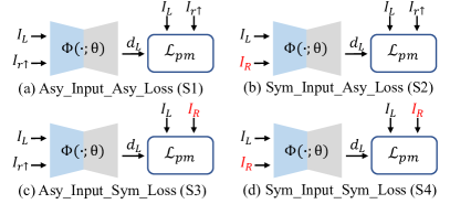
Figure 2: Illustration of four unsupervised stereo matching settings trained with photometric consistency.

Table 1: 3PE (%) results of different unsupervised stereo matching settings on the Inria_SLFD dataset.

Setting	Asymmetric Factor $s$
	2	4	6	8
Asy_Input_Asy_Loss (S1)	7.28	12.56	22.72	27.93
Sym_Input_Asy_Loss (S2)	7.22	10.01	16.31	21.93
Asy_Input_Sym_Loss (S3)	6.38	6.39	6.58	7.52
Sym_Input_Sym_Loss (S4)	6.32

As shown in Fig. 2, a total of four settings of unsupervised stereo matching are evaluated, among which only the first one (S1) can be achieved in practice and the rest ones (S2, S3, and S4) can be regarded as “ideal cases” since the HR right view is used. We select two views of each scene from the Inria_SLFD dataset [32] as the HR left and right views, i.e., $I_{L}$ and $I_{R}$. The LR right view $I_{r}$ is simulated from $I_{R}$ with bicubic downsampling under four asymmetric factors ($s$ = 2, 4, 6, 8). We adopt the popular PSMNet [5] as the backbone network $\Phi(\cdot;\theta)$ and the photometric loss $\mathcal{L}_{pm}$ is computed following Eq. (3) with $\alpha=3$. A standard stereo matching metric, 3-Pixel-Error (3PE) [28], is used to evaluate the performance of different settings (see more implementation details in Sec. 5).

As can be seen from Table 1, when the images input to the feature extractor change from asymmetric to symmetric (S1 to S2), the performance improvements are rather limited (e.g., 2.55% when $s$ = 4). In contrast, when the images used to compute the photometric loss change from asymmetric to symmetric (S1 to S3), the results see a large improvement (e.g., 6.24% when $s$ = 4), which are even close to the upper bound (S4). It is worth emphasizing that, for S1 and S3, the disparity maps used to warp the right view are from the same input and the same network. This phenomenon can be observed under all asymmetric factors. It clearly demonstrates that, for resolution-asymmetric stereo matching, the asymmetry during loss computation has a dominant influence rather than the asymmetry of the input.

A possible solution to make up the photometric inconsistency is to restore the LR right view $I_{r\uparrow}$ through SR techniques to approach $I_{R}$. However, for diverse real-world systems, neither the realistic pair of ($I_{r\uparrow}$, $I_{R}$) nor the explicit degradation from $I_{R}$ to $I_{r\uparrow}$ can be easily available to train SR models. Therefore, this solution may perform decently on properly simulated data but lose efficacy in practice. In view of the results in Table 1, we propose to conquer the challenge of “asymmetric loss” from a new perspective, by projecting $I_{L}$ and $I_{r\uparrow}$ to a feature space that is agnostic to degradation and specific for matching. On the one hand, a degradation-agnostic space can establish another kind of consistency (i.e., feature-metric consistency) to avoid the photometric inconsistency. On the other hand, a matching-specific space can assign different values to pixels belonging to different scene points and thus is suitable for penalizing incorrect matchings. Now the remaining question is: how to learn the desirable feature space?

4 Resolution-asymmetric Stereo Matching

4.1 Feature Space Investigation

Recalling the results in Table 1, it reveals that the feature extractor of a stereo matching network trained under the setting of S3 performs well in extracting symmetric features from the asymmetric input. Although S3 is not attainable in practice, it suggests a potential substitute, i.e., the feature extractor of S1 that takes the same input, for obtaining the desirable feature space. To validate this speculation, we conduct another series of experiments. Besides S1, we investigate two other representative feature spaces used for geometry tasks: 1) a feature network trained with the Contrastive Loss (denoted as CL) as in [35], and 2) the encoder of an Auto-Encoder network (denoted as AE) as in [34]. Details of these two networks are provided in the supplement. All the above networks are pre-trained on the Inria_SLFD dataset with $s$ = 4. Additionally, we also include the original image space for comparison.

We evaluate the degradation-agnostic property of different spaces by computing the PSNR metric between the feature maps extracted from $I_{R}$ and its degraded version $I_{r\uparrow}$ by the corresponding networks. The PSNR in the image space is computed based on pixel intensities. Note that the values in different spaces are normalized to $[0,1]$ to make the comparison of PSNR results meaningful. On the other hand, for the matching-specific property, we perform matching between the feature maps extracted from $I_{L}$ and $I_{r\uparrow}$ directly in different spaces. Specifically, we formulate a matching cost by computing the euclidean distance of two feature vectors at a given disparity. Then a disparity map is obtained by selecting the minimal matching cost at each location following the Winner-Takes-All strategy. For the image space, we perform matching on a 5$\times$5 patch basis. The 3PE metric is then used to evaluate the obtained disparity map.

Table 2: Evaluation of the degradation-agnostic property in PSNR (dB) and the matching-specific property in 3PE (%) of different spaces on the Inria_SLFD dataset.

	Image	CL	AE	S1
PSNR $\uparrow$	24.65	44.18	23.23	28.00
3PE $\downarrow$	55.3	68.90	39.22	20.91

Table 2 gives the PSNR and 3PE results of different spaces. Although CL presents the highest PSNR value, it performs worst in terms of 3PE. In other words, CL is most degradation-agnostic but least matching-specific, which can be attributed to the blur feature maps extracted by the feature network. AE can learn relatively discriminative features for matching thanks to the regularization losses, but it does not impose the consistency between the feature maps of $I_{R}$ and $I_{r\uparrow}$, resulting in the lowest PSNR value. Compared with the image space where the photometric consistency is damaged by the degradation, the feature space of S1 can assign more consistent features for $I_{R}$ and $I_{r\uparrow}$ (with a notably higher PSNR value). Meanwhile, this feature space is more discriminative for performing matching between $I_{L}$ and $I_{r\uparrow}$ than others (with the best 3PE result). In conclusion, we verify that the feature extractor of a stereo matching network can approach the desirable feature space, even trained with the “asymmetric loss”. More analysis on this part and the visualization of different feature maps are provided in the supplement.

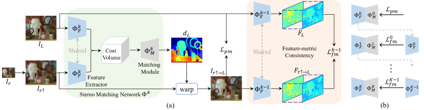
Figure 3: The proposed resolution-asymmetric stereo matching method. (a) The feature extractor $\Phi_{F}$ of a stereo matching network $\Phi$ is utilized to establish the feature-metric consistency and formulate a feature-metric loss $\mathcal{L}_{fm}$. (b) A self-boosting strategy is introduced to progressively strengthen the feature-metric consistency and continuously boost the network $\Phi$. Specifically, $\Phi_{F}^{k-1}$ obtained in the previous stage formulates $\mathcal{L}_{fm}^{k-1}$ to train $\Phi^{k}$ in the current stage, and the initial $\Phi_{F}^{0}$ is trained with the photometric loss $\mathcal{L}_{pm}$.

4.2 Learning with Feature-metric Consistency

Fig. 3 illustrates our proposed method for resolution-asymmetric stereo matching, which follows the typical pipeline of unsupervised learning as described in Sec. 3.1. Note that the focus of this work is not to design a specific stereo matching network but to realize the feature-metric consistency to avoid the photometric inconsistency. Therefore, we adopt the popular PSMNet [5] as the backbone of the stereo matching network, which can be readily replaced by other embodiments (see Sec. 7 for the embodiment of iResNet [22]).

As illustrated in Fig. 3(a), the stereo matching network $\Phi(\cdot;\theta_{F},\theta_{M})$ is comprised of a feature extractor $\Phi_{F}(\cdot;\theta_{F})$ and a matching module $\Phi_{M}(\cdot;\theta_{M})$. Given a stereo pair $I_{L}$ and $I_{r\uparrow}$, $\Phi_{F}(\cdot;\theta_{F})$ extracts degradation-agnostic and matching-specific features $F_{L}=\Phi_{F}(I_{L};\theta_{F})$ and $F_{r\uparrow}=\Phi_{F}(I_{r\uparrow};\theta_{F})$, which are supposed to be consistent at corresponding asymmetric pixels ($\textit{{p}}_{L}$ and $\textit{{p}}_{r\uparrow}$), i.e.,

$$F_{L}[\textit{{p}}_{L}]=F_{r\uparrow}[\textit{{p}}_{r\uparrow}].\vspace{-1mm}$$ (4)

Then, the features $F_{L}$ and $F_{r\uparrow}$ are concatenated into a cost volume that is regularized by $\Phi_{M}(\cdot;\theta_{M})$ to regress a disparity map $d_{L}$.

According to the investigation in Sec. 4.1, we propose to use the feature extractor of the stereo matching network itself to produce the desirable feature space for computing a feature-metric loss. Specifically, after obtaining the warped left view $I_{r\uparrow\rightarrow L}$ with $d_{L}$, the feature extractor $\Phi_{F}(\cdot;\theta_{F})$ is used to project $I_{L}$ and $I_{r\uparrow\rightarrow L}$ to the feature space, producing $F_{L}$ and $F_{r\uparrow\rightarrow L}=\Phi_{F}(I_{r\uparrow\rightarrow L};\theta_{F})$. Since $F_{L}$ should be well reconstructed by $F_{r\uparrow\rightarrow L}$ if $d_{L}$ is estimated accurately, we can formulate the feature-metric loss with the reconstruction error similar to the photometric loss $\mathcal{L}_{pm}$ in Eq. (3), denoted as

$$\mathcal{L}_{fm}=\left\|F_{L}-F_{r\uparrow\rightarrow L}\right\|_{1}+\alpha(1-{\rm SSIM}(F_{L},F_{r\uparrow\rightarrow L})).$$ (5)

4.3 Self-boosting Strategy

As demonstrated in Sec. 4.1, even when the stereo matching network $\Phi(\cdot;\theta_{F},\theta_{M})$ trained with the photometric loss $\mathcal{L}_{pm}$, its feature extractor $\Phi_{F}(\cdot;\theta_{F})$ can approach the desirable feature space. Nonetheless, when the network is trained by a more accurate loss (e.g., $\mathcal{L}_{fm}$), the corresponding $\Phi_{F}(\cdot;\theta_{F})$ extracts more degradation-agnostic and matching-specific features, which can be utilized to strengthen the feature-metric consistency and formulate a better $\mathcal{L}_{fm}$. In return, a better $\mathcal{L}_{fm}$ can further boost $\Phi(\cdot;\theta_{F},\theta_{M})$. To this end, we propose a self-boosting strategy to progressively optimize the feature extractor and continuously boost the network.

Fig. 3(b) illustrates the training process of our method. Given a resolution-asymmetric stereo dataset, we first use $\mathcal{L}_{pm}$ to train a stereo matching network $\Phi(\cdot;\theta_{F}^{0},\theta_{M}^{0})$ (short as $\Phi^{0}$), whose feature extractor $\Phi_{F}^{0}$ formulates a feature-metric loss $\mathcal{L}_{fm}^{0}$. Then, $\mathcal{L}_{fm}^{0}$ is utilized to finetune a new stereo matching network $\Phi^{1}$ which is initialized as $\Phi^{0}$. During the finetuning of $\Phi^{1}$, the feature extractor for computing $\mathcal{L}_{fm}^{0}$ is fixed. After finetuning, a boosted feature extractor $\Phi_{F}^{1}$ formulates a better feature-metric loss $\mathcal{L}_{fm}^{1}$, which is utilized in the next training stage. Following this way, we iteratively finetune $\Phi^{k}$ with the progressively boosted $\mathcal{L}_{fm}^{k-1}$ ($k=1$,…,$K$). Note that we only formulate a new training loss $\mathcal{L}_{fm}^{k}$ when the network $\Phi^{k}$ converges with respect to $\mathcal{L}_{fm}^{k-1}$, since altering the loss space frequently could make the training process unstable. With this self-boosting strategy, we can obtain continuously optimized networks with progressively strengthened feature-metric consistency. The detailed algorithm is provided in the supplement.

Table 3: Validation of the self-boosting strategy on the Inria_SLFD dataset. The 3PE (%) metric is evaluated.

Asymmetric Factor $s$	Stage Number $k$
	0	1	2	3
4	12.56	9.22	7.80	7.70
6	21.47	13.92	10.54	9.88
8	27.93	18.47	14.30	13.30

Table 4: Comparison of different methods on four resolution-asymmetric stereo datasets simulated with an asymmetric factor of 4 and under various degradations. The 3PE (%) / EPE metrics are evaluated. For SR solutions, the results marked gray denote their assumed degradations are inconsistent with the actual ones. The best results are highlighted with bold fonts.

Method	Inria_SLFD					Middlebury
	BIC	IG	AG	IG_JPEG	AG_JPEG	BIC	IG	AG	IG_JPEG	AG_JPEG
SGM	12.41/1.849	16.88/2.316	14.85/2.127	16.93/2.318	14.94/2.134	8.87/1.535	11.70/1.822	10.35/1.696	11.94/1.844	10.60/1.713
BaseNet	12.56/1.680	16.75/2.158	15.27/1.996	16.42/2.029	13.40/1.844	8.72/1.363	9.50/1.482	8.89/1.416	10.27/1.613	8.61/1.414
RCAN+BaseNet	8.89/1.287	14.40/1.842	12.34/1.604	13.94/1.796	12.01/1.612	6.76/1.189	9.14/1.425	7.86/1.287	9.46/1.442	8.72/1.381
DAN+BaseNet	9.91/1.374	10.99/1.464	10.51/1.464	12.97/1.785	11.56/1.583	6.90/1.187	6.70/1.204	7.18/1.231	8.95/1.450	8.35/1.344
BaseNet+CL	12.97/1.700	16.74/2.186	17.36/2.089	17.46/2.236	18.08/2.263	8.13/1.430	11.25/1.649	11.62/1.679	12.45/1.817	10.06/1.631
BaseNet+AE	10.47/1.478	15.17/1.984	13.63/1.840	15.14/1.947	14.29/1.927	6.95/1.244	8.47/1.384	7.80/1.356	9.47/1.459	8.06/1.358
Ours	7.70/1.148	9.01/1.337	8.44/1.249	9.65/1.418	8.47/1.288	5.78/1.088	6.52/1.178	6.38/1.172	7.04/1.204	7.05/1.203
	HCI					KITTI2015
SGM	7.04/1.093	9.85/1.426	8.50/1.273	10.02/1.425	8.62/1.278	30.71/4.001	38.90/5.043	36.01/4.659	39.04/5.040	36.14/4.660
BaseNet	5.95/0.891	9.91/1.213	8.03/1.068	9.82/1.189	7.88/1.083	11.32/2.014	17.37/2.531	13.85/2.243	15.31/2.311	14.66/2.314
RCAN+BaseNet	5.34/0.717	7.23/0.994	6.62/0.893	8.18/1.054	7.70/1.052	9.94/1.846	13.30/2.141	10.98/1.937	13.31/2.162	11.95/2.052
DAN+BaseNet	5.48/0.715	5.32/0.781	6.23/0.830	7.86/0.988	6.56/0.984	10.06/1.938	10.31/1.856	10.31/1.892	12.71/2.089	11.39/1.973
BaseNet+CL	7.80/0.990	8.68/1.124	8.74/1.144	9.35/1.223	8.29/1.137	17.04/2.472	31.03/3.388	20.00/2.676	21.12/2.733	22.30/2.902
BaseNet+AE	5.13/0.818	6.30/1.018	5.51/0.922	7.15/1.079	5.56/0.973	10.53/1.911	15.25/2.316	13.25/2.102	15.05/2.219	13.42/2.122
Ours	4.08/0.637	4.56/0.701	4.21/0.670	4.58/0.719	4.35/0.709	8.66/1.801	10.08/1.901	9.70/1.848	10.62/1.948	9.82/1.874

To validate the proposed strategy, we evaluate the performance of the stereo matching networks at different stages on the Inria_SLFD dataset with $s=4$. As can be seen in Table 3, the network is progressively improved with the increase of stages. It reflects that the feature extractor used in the next stage is boosted and the feature-metric consistency is strengthened. Moreover, with such a strategy, our method remains effective for large degradations. We validate this claim with two larger asymmetric factors ($s$ = 6, 8). As shown in Table 3, the performance of the initial network ($k=0$) significantly deteriorates due to the more severe photometric inconsistency when the asymmetric factor increases. However, the network finally reaches decent performance, thanks to the self-boosting strategy.

5 Experiments on Simulated Datasets

5.1 Datasets and Evaluation Metrics

To quantitatively evaluate the performance of our method, we simulate four resolution-asymmetric stereo datasets, two from the widely used stereo datasets Middlebury [14] and KITTI2015 [28] and two from the light field datasets Inria_SLFD [32] and HCI [16] with a narrow baseline between two views which is closer to the configuration on smartphones. To mimic the diverse degradations in real-world systems, we perform five different degradation operations to synthesize the LR view, including bicubic downsampling (BIC), Isotropic/Anisotropic Gaussian kernel downsampling (IG/AG), and Isotropic/Anisotropic Gaussian kernel downsampling with JPEG compression (IG_JPEG/AG_JPEG). Details of training/testing division of each dataset and generation of different Gaussian kernels are provided in the supplement. For performance evaluation, we adopt two standard metrics for stereo matching, 3-Pixel-Error (3PE) [28] and End-Point-Error (EPE) [27]. 3PE is the percentage of the predicted disparities whose errors are more than 3 pixels and 5% of their ground-truth disparities, while EPE is the average absolute difference between the estimated and ground-truth disparities.

5.2 Comparison Methods

For comparison, we adopt a classical stereo matching method Semi-Global Matching (SGM) [13] and several unsupervised methods that can be divided into two categories. The first category includes three solutions using the photometric loss. Besides the baseline unsupervised network trained under the setting of S1 (denoted as BaseNet) as mentioned in Sec. 3.2, we further use the state-of-the-art non-blind SR method RCAN [48] and blind SR method DAN [26] to super-resolve the LR view as pre-processing, denoted as RCAN+BaseNet and DAN+BaseNet, respectively. The RCAN model is trained under the BIC degradation on a large-scale dataset DIV2K [1] for SR, while the DAN model is trained under a set of degradations including BIC, IG, and AG on DIV2K. The second category includes two feature-metric learning methods [34, 35] that also adopt the baseline network but impose feature-metric consistency in respective feature spaces as mentioned in Sec. 4.1, denoted as BaseNet+CL and BaseNet+AE, respectively. Note that, unless SR models are used, bicubic interpolation is applied to upsample the LR view.

The backbone network of all learning-based solutions is the popular PSMNet [5]. The network is optimized with the ADAM solver ($\beta_{1}$=$0.9$, $\beta_{1}$=$0.999$). We set the learning rate as 0.001. The smoothness constraint on disparity is enforced by the weighted smoothness loss [19], i.e.,

$$\mathcal{L}_{sm}=\left|\partial_{x}d_{L}\right|e^{-\left|\partial_{x}I_{L}\right|}+\left|\partial_{y}d_{L}\right|e^{-\left|\partial_{y}I_{L}\right|}.\vspace{-1.25mm}$$ (6)

Therefore, the overall loss function of all learning-based solutions can be written as

$$\mathcal{L}=\mathcal{L}_{pm/fm}+\lambda\mathcal{L}_{sm},\vspace{-1.25mm}$$ (7)

where $\lambda$ is a weighting factor and $\mathcal{L}_{pm/fm}$ is either the photometric loss for the methods in the first category or the corresponding feature-metric loss for the methods in the second category and ours. The number of stages $K$ in the self-boosting strategy is set as 3. The detailed architecture of the backbone network and the hyper-parameters of different methods are provided in the supplement.

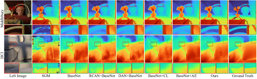
Figure 4: Disparity maps of two exemplar scenes from the Middlebury and HCI datasets. The first scene (Reindeer) is simulated under the IG_JPEG degradation, while the second scene (Pillows) is simulated under the AG_JPEG degradation.

5.3 Results

Quantitative Results. Table 4 shows the comparison results of different methods on four simulated datasets with an asymmetric factor of 4. Compared with methods that do not assume specific degradations (SGM, BaseNet, BaseNet+CL, and BaseNet+AE), our method has a distinct advantage on all datasets and under all degradations. Although BaseNet+CL/AE also resorts to the feature-metric loss, the performance is only comparable or even inferior to BaseNet. It tells that finding a degradation-agnostic and matching-specific feature space is non-trivial. The comparison with the degradation-specific SR solutions RCAN+BaseNet and DAN+BaseNet should be interpreted in twofold. On the one hand, when the actual degradations are consistent with what they assume (BIC for RCAN and BIC/IG/AG for DAN), our method has better performance in most cases yet the improvement is not that large. On the other hand, when the actual degradations are inconsistent with their assumptions (marked gray in Table 4), our method notably surpasses these SR solutions. That is to say, SR solutions will lose efficacy when degradations are unknown in real-world scenarios.

Visual Results. We provide the visual results of two exemplar scenes from the HCI and Middlebury datasets for comparison in Fig. 4. As can be seen, our method obtains more robust results, especially in regions with depth discontinuities. In these regions, correspondence estimation is challenging for the solutions based on photometric consistency, since matching ambiguities could not be resolved even with the help of SR techniques. In contrast, under the feature-metric consistency imposed in a degradation-agnostic and matching-specific feature space, our method better reveals the 3D geometry of testing scenes than BaseNet+CL/AE.

Table 5: Comparison of different methods on datasets simulated with an asymmetric factor of 8 and under the BIC degradation.

Method	Inria_SLFD	HCI	Middlebury	KITTI2015
SGM	34.00/3.979	27.57/3.063	24.72/2.609	57.56/8.83
BaseNet	27.93/2.963	23.21/2.164	15.33/2.049	38.88/4.673
RCAN+BaseNet	21.17/2.442	11.54/1.331	11.28/1.729	25.92/3.159
BaseNet+CL	32.49/3.337	15.16/1.589	16.51/2.129	53.28/5.571
BaseNet+AE	27.11/2.847	12.13/1.450	14.30/2.020	30.81/3.299
Ours	13.30/1.763	6.17/1.008	9.90/1.584	19.10/2.545

Large Asymmetric Factor. To evaluate the performance of different methods under large degradations, we conduct experiments on different datasets simulated with an asymmetric factor of 8 and under the BIC degradation. As can be seen from Table 5, our method surpasses all comparison methods by a large margin, and the improvement is even larger compared with the results in Table 4. For methods using the photometric loss, their performance deteriorates further due to the more severe photometric inconsistency. In contrast, thanks to the self-boosting strategy, our method progressively strengthens the feature-metric consistency and thus maintains superior performance.

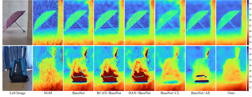
Figure 5: Disparity maps of two exemplar scenes from the self-collected real-world dataset. The colorbars show the value of disparity.

Table 6: Comparison with supervised learning on the Middlebury and KITTI2015 datasets simulated with an asymmetric factor of 4 and under the IG degradation.

Training	Testing	BaseNet-su	BaseNet	Ours
Middlebury	Middlebury	4.05/0.906	9.50/1.482	6.52/1.178
Middlebury	KITTI2015	19.46/3.965	16.98/2.541	13.14/2.280

Comparison with Supervised Learning. The focus of this work is unsupervised learning that does not require ground-truth disparity labels during training and is more robust to be deployed in diverse real-world systems. To verify this point, we also implement a supervised method, which uses the same backbone network as ours but leverages the ground-truth disparity to compute a smooth $L_{1}$ loss [5] (denoted as BaseNet-su). We conduct experiments on the Middlebury and KITTI2015 datasets with an asymmetric factor of 4 under the IG degradation. For both datasets, the networks are trained on Middlebury. Since KITTI2015 consists of street scenes while Middlebury consists of indoor scenes, these two datasets have a large domain gap. As shown in Table 6, when trained on Middlebury and tested on the same dataset, BaseNet-su has the best performance, which is reasonable. However, when trained on Middlebury and tested on KITTI2015, the supervised method loses efficacy and our method achieves notably better generalization, demonstrating the robustness of our method in real-world scenarios where the disparity labels are not available for training.

Table 7: Investigation on the backbone network. * indicates PSMNet [5] is replaced by iResNet [22]. Datasets are simulated with an asymmetric factor of 4 under the BIC degradation.

Method	Inria_SLFD	HCI	Middlebury	KITTI2015
BaseNet∗	18.80/2.411	18.58/1.964	10.92/1.769	17.82/2.549
Ours∗	9.83/1.407	5.83/0.866	8.39/1.382	10.86/1.960

Investigation on the Backbone Network. Besides PSMNet that adopts 3D convolution layers, we also investigate iResNet [22] as another embodiment of the backbone network of our method, which is purely based on 2D convolution layers. Experiments are conducted under the BIC degradation with an asymmetric factor of 4. As shown in Table 7, the iResNet version of our method shows significant gains over the baseline network trained with the photometric loss on all datasets. It demonstrates that the feature extractor of iResNet also learns degradation-agnostic and matching-specific features, which can be used to establish the feature-metric consistency. In other words, the effectiveness of our method is independent of the backbone network used.

6 Experiments on a Real-world Dataset

Dataset Preparation. To validate the performance of our method in real-world systems, we collect a resolution-asymmetric stereo dataset with real degradations. The asymmetric stereo pairs are captured with a Huawei P30 smartphone. This smartphone is equipped with a tele-wide camera system, including a 27mm-equivalent primary lens and an 80mm-equivalent tele-photo lens. The asymmetric factor is approximately equal to 3. After camera calibration and stereo rectification, we capture 30 asymmetric stereo pairs for indoor and outdoor scenes. We randomly split 5 pairs as the testing set and the others as the training set.

Results. As shown in Fig. 5, our method achieves the best visual quality in comparison with the competitors. Similar to the results on simulated datasets, our method estimates much sharper edges and better separates the objects belonging to different depth levels. This advantage is essential to downstream applications, such as bokeh [38] and 3D photography [33]. In contrast, methods using the photometric loss replicate some undesired textures from input images to the estimated disparity maps (e.g., the surface of the umbrella), which is mainly caused by the photometric inconsistency during stereo matching. Both SR solutions show negligible improvements over the baseline network, since their degradation assumptions deviate from the real ones. In addition, the other two methods using the feature-metric loss generate unsatisfactory results due to their incompetent feature spaces. More results are provided in the supplement.

7 Limitation and Conclusion

Limitation. Besides resolution, there might exist other kinds of asymmetry (e.g., color and brightness) when capturing stereo images with a tele-wide camera system, due to the inherent optical differences of two lenses. When collecting the real-world dataset, we manually adjust ISO, exposure time, and white balance of two lenses to mitigate these issues. Although they can be further alleviated through an explicit color and brightness correction after global registration, it remains an open problem whether other kinds of asymmetry can be directly addressed by extending the proposed method. We will consider it as future work.

Conclusion. In this paper, we reveal the main challenge of unsupervised correspondence estimation from resolution-asymmetric stereo images, i.e., the violation of photometric consistency. To conquer this challenge, we realize the feature-metric consistency in an effective and efficient way and introduce a self-boosting strategy to strengthen this consistency. As validated by comprehensive experiments, our method demonstrates superior performance in dealing with various degradations between two views in practice.

References

- [1] Eirikur Agustsson and Radu Timofte. Ntire 2017 challenge on single image super-resolution: Dataset and study. In CVPR Workshops, 2017.
- [2] Filippo Aleotti, Fabio Tosi, Li Zhang, Matteo Poggi, and Stefano Mattoccia. Reversing the cycle: self-supervised deep stereo through enhanced monocular distillation. In ECCV, 2020.
- [3] Adrian Bulat, Jing Yang, and Georgios Tzimiropoulos. To learn image super-resolution, use a gan to learn how to do image degradation first. In ECCV, 2018.
- [4] Jianrui Cai, Hui Zeng, Hongwei Yong, Zisheng Cao, and Lei Zhang. Toward real-world single image super-resolution: A new benchmark and a new model. In CVPR, 2019.
- [5] Jia-Ren Chang and Yong-Sheng Chen. Pyramid stereo matching network. In CVPR, 2018.
- [6] Chang Chen, Zhiwei Xiong, Xinmei Tian, Zheng-Jun Zha, and Feng Wu. Camera lens super-resolution. In CVPR, 2019.
- [7] Jingwen Chen, Jiawei Chen, Hongyang Chao, and Ming Yang. Image blind denoising with generative adversarial network based noise modeling. In CVPR, 2018.
- [8] Xuelian Cheng, Yiran Zhong, Mehrtash Harandi, Yuchao Dai, Xiaojun Chang, Hongdong Li, Tom Drummond, and Zongyuan Ge. Hierarchical neural architecture search for deep stereo matching. In NeurIPS, 2020.
- [9] Zhen Cheng, Zhiwei Xiong, Chang Chen, Dong Liu, and Zheng-Jun Zha. Light field super-resolution with zero-shot learning. In CVPR, 2021.
- [10] Chao Dong, Chen Change Loy, Kaiming He, and Xiaoou Tang. Learning a deep convolutional network for image super-resolution. In ECCV, 2014.
- [11] Geoffrey Egnal. Mutual information as a stereo correspondence measure. 2000.
- [12] Yong Seok Heo, Kyong Mu Lee, and Sang Uk Lee. Robust stereo matching using adaptive normalized cross-correlation. IEEE Transactions on Pattern Analysis and Machine Intelligence, 33(4):807–822, 2010.
- [13] Heiko Hirschmuller. Stereo processing by semiglobal matching and mutual information. IEEE Transactions on Pattern Analysis and Machine Intelligence, 30(2):328–341, 2007.
- [14] Heiko Hirschmuller and Daniel Scharstein. Evaluation of cost functions for stereo matching. In CVPR, 2007.
- [15] Heiko Hirschmuller and Daniel Scharstein. Evaluation of stereo matching costs on images with radiometric differences. IEEE Transactions on Pattern Analysis and Machine Intelligence, 31(9):1582–1599, 2008.
- [16] Katrin Honauer, Ole Johannsen, Daniel Kondermann, and Bastian Goldluecke. A dataset and evaluation methodology for depth estimation on 4d light fields. In ACCV, 2016.
- [17] Yukun Huang, Zheng-Jun Zha, Xueyang Fu, Richang Hong, and Liang Li. Real-world person re-identification via degradation invariance learning. In CVPR, 2020.
- [18] Alex Kendall, Hayk Martirosyan, Saumitro Dasgupta, Peter Henry, Ryan Kennedy, Abraham Bachrach, and Adam Bry. End-to-end learning of geometry and context for deep stereo regression. In ICCV, 2017.
- [19] Ang Li and Zejian Yuan. Occlusion aware stereo matching via cooperative unsupervised learning. In ACCV, 2018.
- [20] Yue Li, Yueyi Zhang, and Zhiwei Xiong. Revisiting flipping strategy for learning-based stereo depth estimation. In VCIP, 2021.
- [21] Mingyang Liang, Xiaoyang Guo, Hongsheng Li, Xiaogang Wang, and You Song. Unsupervised cross-spectral stereo matching by learning to synthesize. In AAAI, 2019.
- [22] Zhengfa Liang, Yiliu Feng, Yulan Guo, Hengzhu Liu, Wei Chen, Linbo Qiao, Li Zhou, and Jianfeng Zhang. Learning for disparity estimation through feature constancy. In CVPR, 2018.
- [23] Anran Liu, Yihao Liu, Jinjin Gu, Yu Qiao, and Chao Dong. Blind image super-resolution: A survey and beyond. arXiv preprint arXiv:2107.03055, 2021.
- [24] Rui Liu, Chengxi Yang, Wenxiu Sun, Xiaogang Wang, and Hongsheng Li. Stereogan: Bridging synthetic-to-real domain gap by joint optimization of domain translation and stereo matching. In CVPR, 2020.
- [25] Yicun Liu, Jimmy Ren, Jiawei Zhang, Jianbo Liu, and Mude Lin. Visually imbalanced stereo matching. In CVPR, 2020.
- [26] Zhengxiong Luo, Yan Huang, Shang Li, Liang Wang, and Tieniu Tan. Unfolding the alternating optimization for blind super resolution. In NeurIPS, 2020.
- [27] Nikolaus Mayer, Eddy Ilg, Philip Hausser, Philipp Fischer, Daniel Cremers, Alexey Dosovitskiy, and Thomas Brox. A large dataset to train convolutional networks for disparity, optical flow, and scene flow estimation. In CVPR, 2016.
- [28] Moritz Menze and Andreas Geiger. Object scene flow for autonomous vehicles. In CVPR, 2015.
- [29] Kuang-Yu Pan and Yung-Yu Chuang. Continuous zoom with two fixed-focal-length lens. In SIGGRAPH ASIA 2016 Posters.
- [30] Jiayong Peng, Zhiwei Xiong, Yicheng Wang, Yueyi Zhang, and Dong Liu. Zero-shot depth estimation from light field using a convolutional neural network. IEEE Transactions on Computational Imaging, 6:682–696, 2020.
- [31] Daniel Scharstein and Richard Szeliski. A taxonomy and evaluation of dense two-frame stereo correspondence algorithms. International journal of computer vision, 47(1):7–42, 2002.
- [32] Jinglei Shi, Xiaoran Jiang, and Christine Guillemot. A framework for learning depth from a flexible subset of dense and sparse light field views. IEEE Transactions on Image Processing, 28(12):5867–5880, 2019.
- [33] Meng-Li Shih, Shih-Yang Su, Johannes Kopf, and Jia-Bin Huang. 3d photography using context-aware layered depth inpainting. In CVPR, 2020.
- [34] Chang Shu, Kun Yu, Zhixiang Duan, and Kuiyuan Yang. Feature-metric loss for self-supervised learning of depth and egomotion. In ECCV, 2020.
- [35] Jaime Spencer, Richard Bowden, and Simon Hadfield. Defeat-net: general monocular depth via simultaneous unsupervised representation learning. In CVPR, 2020.
- [36] Alessio Tonioni, Fabio Tosi, Matteo Poggi, Stefano Mattoccia, and Luigi Di Stefano. Real-time self-adaptive deep stereo. In CVPR, 2019.
- [37] Marc Comino Trinidad, Ricardo Martin Brualla, Florian Kainz, and Janne Kontkanen. Multi-view image fusion. In ICCV, 2019.
- [38] Neal Wadhwa, Rahul Garg, David E Jacobs, Bryan E Feldman, Nori Kanazawa, Robert Carroll, Yair Movshovitz-Attias, Jonathan T Barron, Yael Pritch, and Marc Levoy. Synthetic depth-of-field with a single-camera mobile phone. ACM Transactions on Graphics, 37(4):1–13, 2018.
- [39] Longguang Wang, Yulan Guo, Yingqian Wang, Zhengfa Liang, Zaiping Lin, Jungang Yang, and Wei An. Parallax attention for unsupervised stereo correspondence learning. IEEE Transactions on Pattern Analysis and Machine Intelligence, 2020.
- [40] Lizhi Wang, Zhiwei Xiong, Guangming Shi, Wenjun Zeng, and Feng Wu. Simultaneous depth and spectral imaging with a cross-modal stereo system. IEEE Transactions on Circuits and Systems for Video Technology, 28(3):812–817, 2018.
- [41] Tengfei Wang, Jiaxin Xie, Wenxiu Sun, Qiong Yan, and Qifeng Chen. Dual-camera super-resolution with aligned attention modules. In ICCV, 2021.
- [42] Yang Wang, Yang Cao, Zheng-Jun Zha, Jing Zhang, and Zhiwei Xiong. Deep degradation prior for low-quality image classification. In CVPR, 2020.
- [43] Yicheng Wang, Jiayong Peng, Yueyi Zhang, Shan Liu, Xiaoyan Sun, and Zhiwei Xiong. Asymmetric stereo color transfer. In ICME, 2021.
- [44] Li Xu and Jiaya Jia. Two-phase kernel estimation for robust motion deblurring. In ECCV, 2010.
- [45] Mingde Yao, Zhiwei Xiong, Lizhi Wang, Dong Liu, and Xuejin Chen. Spectral-depth imaging with deep learning based reconstruction. Optics express, 27(26):38312–38325, 2019.
- [46] Huangying Zhan, Ravi Garg, Chamara Saroj Weerasekera, Kejie Li, Harsh Agarwal, and Ian Reid. Unsupervised learning of monocular depth estimation and visual odometry with deep feature reconstruction. In CVPR, 2018.
- [47] Xuaner Zhang, Qifeng Chen, Ren Ng, and Vladlen Koltun. Zoom to learn, learn to zoom. In CVPR, 2019.
- [48] Yulun Zhang, Kunpeng Li, Kai Li, Lichen Wang, Bineng Zhong, and Yun Fu. Image super-resolution using very deep residual channel attention networks. In ECCV, 2018.
- [49] Tiancheng Zhi, Bernardo R Pires, Martial Hebert, and Srinivasa G Narasimhan. Deep material-aware cross-spectral stereo matching. In CVPR, 2018.
- [50] Yiran Zhong, Yuchao Dai, and Hongdong Li. Self-supervised learning for stereo matching with self-improving ability. arXiv preprint arXiv:1709.00930, 2017.
- [51] Chao Zhou, Hong Zhang, Xiaoyong Shen, and Jiaya Jia. Unsupervised learning of stereo matching. In ICCV, 2017.
- [52] Shenglong Zhou, Zhiwei Xiong, Chang Chen, Xuejin Chen, Dong Liu, Yueyi Zhang, Zheng-Jun Zha, and Feng Wu. Fast and accurate electron microscopy image registration with 3d convolution. In MICCAI, 2019.