The rotation of planet-hosting stars

Abstract

Understanding the distribution of angular momentum during the formation of planetary systems is a key topic in astrophysics. Data from the Kepler and Gaia missions allow to investigate whether stellar rotation is correlated with the presence of planets around Sun-like stars. Here, we perform a statistical analysis of the rotation period of 493 planet-hosting stars. These are matched to a control sample, without detected planets, with similar effective temperatures, masses, radii, metallicities, and ages. We find that planet-hosting stars rotate on average $1.63\pm 0.40$ days slower. The difference in rotation is statistically significant both in samples including and not including planets confirmed by radial velocity follow-up observations. We also analyse the dependence of rotation distribution on various stellar and planetary properties. Our results could potentially be explained by planet detection biases depending on the rotation period of their host stars in both RV and transit methods. Alternatively, they could point to a physical link between the existence of planets and stellar rotation, emphasising the need to understand the role of angular momentum in the formation and evolution planetary systems.

1 Introduction

The Sun contains more than 99% of the mass of the solar system, but less than 1% of its angular momentum (e.g., Ray2012). In fact, most of the current angular momentum of the solar system is located in the gas giants, Jupiter and Saturn, due to their high masses and large orbital distances. The different distribution of angular momentum and mass is largely a consequence of angular momentum transport processes during the protoplanetary disk phase (e.g., 2011ARA&A..49...67W).

The discovery of thousands of planets around other stars provides the opportunity to characterise the properties of planetary systems in a statistically robust manner. Ground based observations and space missions such as CoRoT (Baglin2003), Kepler (Borucki2010; Koch2010) and TESS (Ricker2015) have quantified the radii, masses, and orbits of many exoplanets as well as the properties of their host stars. These new data make it possible to explore whether the properties of planet-hosting stars differ from those without planets. A question of interest is whether the angular momentum of stars is correlated with the occurrence of (massive) planets, i.e., do stars that host (massive) planets rotate slower than those without planets?

Theoretical works have not studied this question directly, but focused on rotational evolution during the pre-main sequence phase and on star-planet interactions. For instance, tidal interactions have been suggested to result in spin-down of initially fast-rotating stars (e.g. Bolmont2016), while magnetic and tidal effects may lead to planets migrating or even colliding with the star, affecting the stellar rotation (e.g. Ahuir2019).

Observationally, this topic has been investigated and no clear trend has been found. For example, while Ceillier2015 found no effect of the presence of small planets on their host star’s rotation, Alves2010 suggested that stars with planets exhibit a surplus of angular momentum compared to stars without planets. In contrast, Berget2010; Gonzalez2015 report that planet hosts tend to spin slower than similar stars without planets. In addition to these studies, PazChinchon2015 confirm a trend between stellar angular momentum and stellar mass (the Kraft relation, Kraft1967). Finally, Gurumath2019 report a dependence of planetary orbital angular momentum on planetary mass, and that this dependence differs between single and multiple planetary systems.

The Kepler mission has detected more than 2400 transiting exoplanets around Sun-like stars, providing us with numerous planetary radii and orbital periods. Moreover, the Gaia Data Release 2 (GAIA2016; Gaia2018; Arenou2018; Lindegren2018) has allowed the determination of stellar properties for a large number of stars with unprecedented precision. In this work we create a homogeneously derived catalog based on Kepler and Gaia data including various stellar (Berger2020) and planetary (NASA exoplanet archive) properties, as well as stellar rotation periods (McQuillan2013b; McQuillan2014) to investigate the correlation between planet occurrence and stellar rotation.

Our paper is organised as follows. We detail our methods in section 2. Our results are presented in section 3, where we first show the influence of the presence of a planet, and then investigate the dependence on stellar and planetary properties. We discuss our results and conclude in LABEL:sec:discussion.

2 Methods

In this study, we combine rotation period measurements from McQuillan2013b and McQuillan2014 with other fundamental stellar properties derived homogeneously by Berger2020, to obtain a large dataset of 32,049 stars (493 with and 31,556 without detected planets). This dataset is large enough to infer statistically significant results. Furthermore, the homogeneously derived properties from Berger2020 make our datasets as self-consistent as possible, instead of combining data from many different sources. Measurement uncertainties are taken into account by bootstrapping the data. We then match the non-rotational properties of the two populations in order to remove biases related to the non-rotational stellar properties. This allows us to isolate a potential correlation between planet occurrence and stellar rotation. We also study the dependence of this correlation on stellar and planetary parameters.

We compare the rotation periods of stars with planets and stars without planets. The first step is to establish these two datasets: (i) stars with detected planets and (ii) stars without detected planets. More details can be found in Appendix LABEL:Appendix1. The stellar parameters we use are the stellar effective temperature $T_{\rm{eff}}$, mass $M_{s}$, radius $R_{s}$, metallicity [Fe/H], age $t_{\rm{age}}$, and rotation period $P_{\rm{rot}}$.

2.1 Datasets

In order for the datasets to be self-consistent, we want as few parameter sources as possible. Rotation periods are obtained from McQuillan2013b; McQuillan2014, which provide periods for 737 Kepler Objects of Interest (KOI) and 34,030 Kepler targets respectively. The methods used by the authors to determine the rotation periods are described in McQuillan2013a.
We collect all other parameters from Berger2020, where the stellar properties for 186,301 Kepler stars are determined from isochrones and broadband photometry, Gaia Data Release 2 (Arenou2018; GAIA2016; Gaia2018; Lindegren2018) parallaxes, and spectroscopic metallicities, where available (for more details on their methods, see Howes2019). A “goodness-of-fit" (GOF) parameter is supplied for each star and Berger2020 consider those with GOF<0.99 to have unreliable ages, and therefore we remove them from the datasets.
The planets’ properties are taken from the NASA exoplanet archive (consulted on the 27th of April, 2020). Since we focus on transiting systems, the properties are the planetary radius $R_{p}$ and orbital period $P_{\rm{orb}}$, as well as the number of planets detected in each system (multiplicity).
We cross-reference the two stellar catalogues by KIC identification number. We separate the stars from McQuillan2013b (KOIs) that appear in the NASA exoplanet archive to make the set of stars with planets, and the rest of the stars make up the control sample. The final dataset contains 32,049 stars, split into 493 stars with and 31,556 stars without confirmed planets. Table 1 shows the distribution of spectral types of the planet-hosting stars in the dataset.

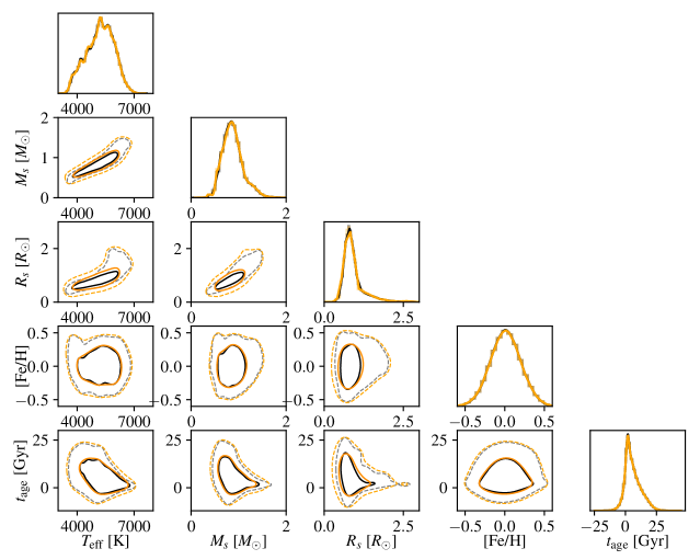
Figure 1: Distributions of the various non-rotational stellar properties both for the bootstrapped planet-hosting stars and for the matched control sample. Diagonal plots show one-dimensional probability distribution functions of the two data sets, while off-diagonal plots show two-dimensional distributions. In each panel, orange (black) lines and points represent stars with (without) detected planets. Contour lines enclose 68% (solid) and 95% (dashed) of all the stars.

Table 1: Number of planet-hosting stars belonging to each spectral type.

Spectral type	$T_{\rm{eff}}$	Number of stars
F	6000 - 7500	68
G	5000 - 6000	244
K	3500 - 5000	180
M	2500 - 3500	1

2.2 Bootstrapping and matching processes

The subset of stars with confirmed planets is not a representative sample of the total stellar population. Indeed, both physical effects and observational biases lead to differences in those populations’ properties. We can evoke for example the widely accepted correlation between giant planet occurrence and stellar metallicity (Gonzalez1997; Santos2004; Fischer2005; Mortier2013), as well as the bias of the transit method towards stars of smaller radii. Our aim is to investigate whether, all else being equal, planet occurrence is correlated with stellar rotation. Thus, in order to remove those effects and compare apples to apples, we match each planet-hosting star with the most similar star in the control sample. By its nature, our matching procedure can only correct for biases of the non-rotational stellar properties but not those linked to that of the stellar rotation.

The stellar rotation periods are provided with $1\sigma$ errors by McQuillan2013b; McQuillan2014, and the average relative error of the full cross-referenced sample is $\frac{\sigma(P_{\rm{rot}})}{P_{\rm{rot}}}=2.7\%$. The errors on the other stellar parameters ($T_{\rm{eff}}$, $M_{s}$, $R_{s}$, [Fe/H], and $t_{\rm{age}}$) are given as upper and lower values by Berger2020, and we keep the larger one of the two as the $1\sigma$ uncertainty. The resulting average relative errors on non-rotational parameters are:

$$\hskip 30.0pt\frac{\sigma(T_{\rm{eff}})}{T_{\rm{eff}}}=1.9\%,~{}\frac{\sigma(M_{s})}{M_{s}} =5.9\%,~{}\frac{\sigma(R_{s})}{R_{s}}=4.2\%,$$

$$\frac{\sigma(\text{[Fe/H]})}{\text{[Fe/H]}}=34.1\% ,~{}\text{and}~{}\frac{\sigma(t_{\rm{age}})}{t_{\rm{age}}}=78.5\%.$$

First, we bootstrap both datasets within the uncertainty ranges of each stellar parameter. We sample every star (both with and without planets) 1000 times assuming a normal distribution on each parameter, with the standard deviation corresponding to the measurement uncertainties. We thus end up with 1000 samples of the two datasets. For every one of these 1000 samples, we use a multidimensional Euclidean distance based on the non-rotational parameters to match each planet-hosting star to the most similar star without detected planets. We then compare the rotation periods between the stars with and without detected planets. A detailed description of the methods is given in Appendix LABEL:Appendix1.

Figure 1 shows two-dimensional distributions of the various non-rotational stellar properties both for the planet-hosting stars and for the matched control sample showing excellent agreement. In addition, the 1-dimensional distributions of the non-rotational parameters agree well between the two samples, see Table 3, with $p$-values of Kolmogorov-Smirnov tests close to unity. A similar figure for the unmatched datasets can be found in LABEL:fig:pairplots_prematch. Note, however, that contour lines in Figure 1 include the bootstrapping of the measurement errors, while the contour lines in LABEL:fig:pairplots_prematch do not.

Figure 2 shows $P_{\rm rot}$ as a function of the non-rotational stellar properties. The two populations correspond to stars with (orange) and without (black) planets (unmatched). It is clear that regardless to the existence of planets there are correlations between $P_{\rm rot}$ and the other stellar properties. Most significant are the higher $P_{\rm rot}$ for cooler, smaller and low-mass stars (investigated by e.g. McQuillan2014). Also younger stars seem to rotate faster (this is coherent with Kraft1967; Skumanich1972).

Figure 2: Bivariate contour plots of $P_{\rm rot}$ as a function of the non-rotational stellar properties. Orange (black) curves correspond to the final datasets of stars with (without) planets, see subsection 2.1.

Table 2: Pearson and Spearman correlation coefficients between $\log{P_{\rm{rot}}}$ and the non-rotational stellar parameters.

	$\log{T_{\rm{eff}}}$	$\log{M_{s}}$	$\log{R_{s}}$	[Fe/H]	$\log{t_{\rm{age}}}$
Pearson with planets	$-0.501\pm 0.039$	$-0.496\pm 0.039$	$-0.438\pm 0.041$	$0.0516\pm 0.0451$	$0.476\pm 0.040$
Pearson without planets	$-0.485\pm 0.00$5	$-0.488\pm 0.00$5	$-0.433\pm 0.005$	$0.0321\pm 0.006$	$0.378\pm 0.005$
Spearman with planets	$-0.518\pm 0.029$	$-0.481\pm 0.029$	$-0.443\pm 0.029$	$0.086\pm 0.029$	$0.456\pm 0.029$
Spearman without planets	$-0.559\pm 0.003$	$-0.532\pm 0.003$	$-0.501\pm 0.003$	$0.0702\pm 0.003$	$0.393\pm 0.003$

The correlation coefficients for the different stellar properties are given for both datasets of stars.

Our quantity of interest is the average $P_{\rm{rot}}$ difference between stars without planets and planet-hosting stars, $\Delta P_{\rm{rot}}$. It is obtained in the following manner: in each bootstrap iteration i we compute the average of all 493 pairwise differences, $\Delta P_{\rm{rot}}^{i}$. Then the mean and standard deviation over the 1000 $\Delta P_{\rm{rot}}^{i}$ are estimators of the overall average period difference $\Delta P_{\rm{rot}}$ and its error $e(\Delta P_{\rm{rot}})$, respectively.

In order to validate our method, we apply it to a random sample of stars without detected planets, biased in non-rotational parameters. By construction, the selection bias does not depend on stellar rotation, and therefore our method should return a $\Delta P_{\rm rot}$ value that is not statistically significant. This is indeed the result where $\Delta P_{\rm rot}=(0.38\pm 0.35)\text{d}$. Further details on this validation can be found in Appendix LABEL:Appendix2.
Furthermore, a large fraction of Kepler planets have been confirmed with radial velocity (RV) follow-up observations. This could lead to the sample of stars with confirmed planets being biased in stellar rotation. Indeed a radial velocity detection is harder to obtain around a fast-rotating star because of the Doppler broadening induced by stellar rotation. To ensure that this effect is not the cause of the $\Delta P_{\rm rot}$ we detect, we remove from our datasets the stars whose planets have been confirmed by RV (see Appendix LABEL:Appendix3 for further information).

Table 3: Statistical tests on matched datasets.

	$T_{\rm{eff}}$	$M_{s}$	$R_{s}$	[Fe/H]	$t_{\rm{age}}$	$P_{\rm{rot}}$
KS p-value	0.999	0.994	0.950	0.999	0.999	0.00480
KS statistic	0.0214	0.0238	0.0308	0.0195	0.0199	0.123
TT p-value	0.935	0.943	0.934	0.965	0.961	0.0183
TT statistic	-0.0726	0.0251	-0.0229	0.00390	0.00939	2.75
Wilcoxon p-value	0.416	0.479	0.434	0.475	0.503	0.00613
Wilcoxon statistic	57674	58194	57812	58200	58371	50039

Comparison of the distribution of stellar parameters with a Kolmogorov-Smirnov test (first two rows), a Student $t$ test (middle rows), and a Wilcoxon signed-rank test (bottom two rows) for stars with planets and for stars without planets after matching on non-rotational stellar properties. We perform each test for each of the 1000 bootstrap iterations of the matching, and then report the mean statistics.

3 Results

3.1 Influence of the presence of a planet

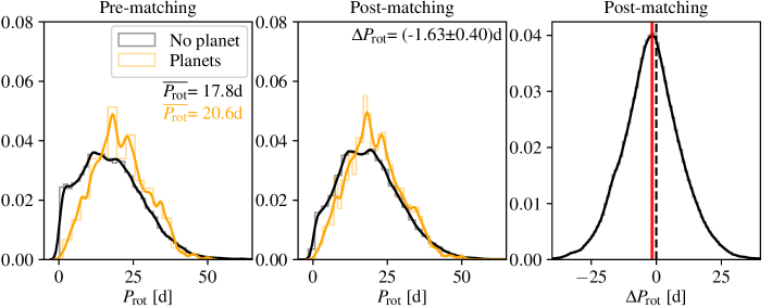
Figure 3: Left panel: Rotation period histograms for stars with one or more detected planets (orange) and stars without detected planets (black), before matching. We give the average rotation period $\overline{P_{\rm rot}}$ of each dataset. Middle panel: Rotation period histograms for stars with planets (orange) and their matched counterparts without detected planets (black). Also shown is the inferred $\Delta P_{\rm{rot}}$ (see Appendix LABEL:Appendix1 for details). Right panel: Histogram of $\Delta P_{\rm{rot}}$ for all 493000 matched pairs of (star with planets, star without planets). The average difference over all samples and iterations is $\Delta P_{\rm{rot}}=(-1.63\pm 0.40)$d (indicated by the red line). The black dashed line corresponds to $\Delta P_{\rm{rot}}=0$.

The main question we aim to answer in this work is whether there is a statistically significant period difference between stars with and without planets. The left panel of Figure 3 shows the distribution of rotation periods of stars with planets (orange) and without detected planets (black). We indicate the average rotation period of each dataset; before matching the average period difference is -3.2 days.

The middle panel of Figure 3 shows the distributions of rotation periods for stars with and without planets, after matching. We show the data for the entire bootstrapped sample of $1000\times 493$ stars with planets and their matched counterparts. After matching, we find a $4\sigma$ result:

$$\Delta P_{\rm{rot}}=(-1.63\pm 0.40)~{}\text{days}.$$ (1)

This shows that the stars with planets rotate on average 1.6 days slower than those without, all else being equal. We clearly see that, although the two matched populations are very similar in their non-rotational properties (see Figure 1), the rotation period distributions are very different. The p-values for $P_{\rm{rot}}$, shown in Table 3 are $4.8\times 10^{-3}$ for the KS test and $1.8\times 10^{-2}$ for the t-test. The right panel of Figure 3 shows the distribution of period differences among matched pairs of (star with planets, star without planets) counterparts. The red line represents the result $\Delta P_{\rm{rot}}=(-1.63\pm 0.40)~{}\text{days}$, and the black dashed line indicates $\Delta P_{\rm{rot}}=0$.

The reported metallicities of many targets in our dataset are not based on spectroscopic measurements and therefore their values are somewhat uncertain. In order to check the importance of the metallicity values on our results, we have cross-matched our catalogue with the LAMOST catalogue (LAMOST2012, LAMOST DR7), yielding 133 stars with and 6075 stars without detected planets. Applying our method on these two datasets, we find $\Delta P_{\rm rot}=(-1.58\pm 0.70)~{}$days, in very good agreement with the result obtained using all stellar properties from Berger2020.
Another potential concern relates to stellar ages. While Berger2020 provide a GOF parameter for stellar ages, we still have stars in the dataset with estimated ages of $\gtrsim{}14$ Gyr, as well as stars with relative age uncertainties larger than 100%. Therefore, we perform two different cuts on our datasets. First, we select only the stars with $t_{\rm age}<14$ Gyr and with relative uncertainties smaller than 100%. This yields 264 stars with and 18837 stars without detected planets. For this sample we find $\Delta P_{\rm rot}=(-1.43\pm 0.56)~{}$days. In a second, more stringent, test we consider only stars with relative age uncertainties of less than 50%. This yields 57 stars with and 7394 stars without detected planets. For this data set we get $\Delta P_{\rm rot}=(-3.00\pm 1.19)~{}$days. Both of these results, while less statistically significant, are still in agreement (within 3$\sigma$) with the result we get using the full datasets.
In a further test, we artificially inflate the uncertainties on the stellar rotation periods by a factor of three finding again no significant change in our results. The uncertainties on stellar rotation do not come into play in the matching process (as we match on non-rotational properties), but only in the bootstrapping. This means that changing the uncertainties on stellar rotation does not change which stars get matched to one another. The individual differences in rotation periods between pairs of matched counterparts are changed by inflating the uncertainties, but they average out due to the large number of bootstraps.

3.2 Dependence on stellar properties

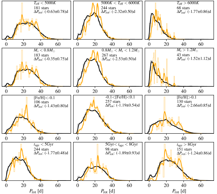
Figure 4: Rotation period histograms (after matching) for stars with and without detected planets in bins of stellar mass, effective temperature, metallicity, and age (from top to bottom). As in previous figures, the orange curves represent stars with planets and the black curves, stars without planets. In each panel we specify the selection criterion, the amount of stars, and the average rotation period difference.

Table 4: $\Delta P_{\rm{rot}}$ as a function of stellar parameters.

Filter	$N_{\rm{stars}}$	$\overline{P_{\rm{rot}}}(\text{with planets})$ [d]	$\overline{P_{\rm{rot}}}(\text{without planets})$ [d]	$\Delta P_{\rm{rot}}$ [d]	p-value
$T_{\rm{eff}}$ < 5000K	181	25.2	24.6	$-0.63\pm 0.78$	0.37
5000K < $T_{\rm{eff}}$ < 6000K	244	19.9	17.6	$-2.34\pm 0.50$	$1.4\times 10^{-5}$
$T_{\rm{eff}}$ > 6000K	68	11.1	9.3	$-1.77\pm 0.86$	0.056
$M_{s}$ < $0.8M_{\odot}$	183	24.8	24.4	$-0.35\pm 0.75$	0.48
$0.8M_{\odot}$ < $M_{s}$ < $1.2M_{\odot}$	267	19.5	16.9	$-2.53\pm 0.50$	$2.2\times 10^{-6}$
$M_{s}$ > $1.2M_{\odot}$	43	10.4	8.8	$-1.52\pm 1.12$	0.075
[Fe/H] < -0.1	106	20.6	19.2	$-1.43\pm 0.80$	0.10
-0.1 < [Fe/H] < 0.1	257	20.0	18.8	$-1.19\pm 0.54$	0.065
[Fe/H] > 0.1	130	21.9	19.3	$-2.66\pm 0.85$	$3.5\times 10^{-3}$
$t_{\rm{age}}$ < 5Gyr	244	17.0	15.3	$-1.77\pm 0.48$	$9.3\times 10^{-4}$
5Gyr < $t_{\rm{age}}$ < 8Gyr	98	22.6	20.7	$-1.89\pm 0.93$	0.054
$t_{\rm{age}}$ > 8Gyr	151	25.2	24.0	$-1.24\pm 0.86$	0.17

We next analyse the rotation period of the stars in the dataset depending on the stellar properties. Specifically, we divide the sample as follows. In terms of mass we split into low-mass ($M_{s}<0.8M_{\odot}$), Sun-like mass ($0.8M_{\odot}<M_{s}<1.2M_{\odot}$), and high-mass ($M_{s}>1.2M_{\odot}$) stars. We also separate the sample according to temperature: Cool ($T_{\rm{eff}}<5000K$), Sun-like effective temperature ($5000K<T_{\rm{eff}}<6000K$), and Hot ($T_{\rm{eff}}>6000K$), metallicity: low ([Fe/H]$<-0.1$), intermediate ($-0.1<$[Fe/H]$<0.1$), and high ([Fe/H]$>0.1$). Finally, we consider the stellar age: young ($t_{\rm{age}}<5$Gyr), intermediate ($5\text{Gyr}<t_{\rm{age}}<8$Gyr), and old ($t_{\rm{age}}>8$Gyr). The distributions of rotation period of the various sub-populations are shown in Figure 4. Interestingly, the average rotation period of massive and hot stars is $\sim$10 days, much shorter than the mean rotation period of the full dataset (this is consistent with Kraft1967; Skumanich1972; McQuillan2014). In the remainder of this section we focus, however, on the difference in rotation period between stars with and without detected planets.

Intermediate-mass stars show a significantly smaller, i.e., more negative, $\Delta P_{\rm rot}\sim{}-2.5\pm{}0.5$d than the entire sample. In other words, stars with mass similar to the Sun do not only rotate slower than similar stars without detected planets but also slower (on average) than low-mass or high-mass stars with detected planets. The same results ($\Delta P_{\rm rot}\sim{}-2.3\pm{}0.5$d) also hold when we split our sample according to effective temperature instead of mass.

As can be seen in the third row of Figure 4 the $P_{\rm rot}$ distributions shifting to higher values (slower rotation) for higher metallicities. This result is consistent with previous studies suggesting that metal-rich stars rotate more slowly than metal-poor stars (e.g. Karoff2018; Amard2020). We also find that metal-rich stars with planets rotate significantly slower than those without ($\Delta P_{\rm rot}\sim{}-2.7\pm{}0.9$d), while intermediate-metallicity stars show a weaker (2-$\sigma$) difference in their rotation periods. Similarly, young stars with planets rotate much slower than young stars without detected planets ($\Delta P_{\rm rot}\sim{}-1.8\pm{}0.5$d). The difference in rotation is also noticeable for intermediate-age stars albeit with a lower statistical significance. The other studied sub-populations do not show strong differences in their average rotation periods. Our findings are summarised in Table 4.

While theoretical models predict that magnetic braking slows down the stellar rotation within a Gyr timescale (e.g. Bouvier2008), recent studies have extended this upper limit due to evidence of older stars having unusually fast rotation (vanSaders2016; Hall2021). We therefore analyse $\Delta P_{\rm rot}$ for stars with different ages. Figure 5 shows $\Delta P_{\rm rot}$ for stars below and above a given age limit ranging from 1 to 3 Gyr. As expected, the magnitude of $\Delta P_{\rm rot}$ decreases for samples with older stars. Interestingly, however, even the sample consisting of stars with ages $>$ 3 Gyr still shows a statistically significant $\Delta P_{\rm rot}$. This observation can be understood from the scaling of the rotation period with stellar age shown in LABEL:fig:Age_vrot_All in the Appendix. While the stellar rotation period increases quickly with age for stars $<1$ Gyr, the slow down in rotation continues up to several Gyr. We note that the relation between stellar age and rotation period shows a large scatter.

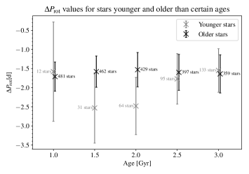
Figure 5: Scatter plot of the $\Delta P_{\rm rot}$ values for stars older and younger than certain ages. The values and uncertainties of $\Delta P_{\rm rot}$ and the corresponding number of stars in each age bin are listed in LABEL:table:deltas_over_under.

Finally, we also separate the sample according to the stellar rotation periods, selecting stars with and without detected planets that have $P_{\rm rot}>2~{}$days, $P_{\rm rot}>7~{}$days, $P_{\rm rot}>15~{}$days, and $P_{\rm rot}<15~{}$days. Removing fast rotators (keeping stars with $P_{\rm rot}>2-7~{}$days) reduces the statistical significant of our result to 2-3$\sigma$. At the same time, when we consider only the stars with $P_{\rm rot}>15~{}$days we find that there is no difference in rotation period. This seems to suggest that our result is strongly affected by the fast-rotating stars in our dataset. There are however two points that make such a selection less than ideal. First, selecting stars according to their rotation period hinders the matching process. Indeed, for our analysis we match stars based on their non-rotational properties. It is then possible for a slow-rotator to be best matched with a fast-rotator, or vice-versa. If however we perform a selection based on rotation period for both stars with and without planets, it is impossible for a slow-rotator to be matched with a fast-rotator, or vice-versa. The effect would be to remove the tails of the distribution of $\Delta P_{\rm rot}$ that we see in the right panel of Figure 3. In other words, the best possible match for a certain star may be removed from the dataset due to the $P_{\rm rot}$ selection process, which leads to a rather large loss of information. Second, $P_{\rm rot}$ is correlated to other stellar properties (see Figure 2 or e.g. McQuillan2014). Selecting only stars with $P_{\rm rot}>15~{}$days biases the samples towards low-mass, colder stars, which exhibit the least significant result, as shown in Figure 4. It is therefore not surprising that our result does not hold for stars with $P_{\rm rot}>15~{}$days.

3.3 Dependence on planetary properties

In this section, we investigate how the rotation periods of stars depend on the properties of their planets. We split our data based on planet multiplicity, orbital period $P_{\rm{orb}}$, and planet radius $R_{p}$ arriving at the following sub-samples. Planetary systems with a ‘distant planet’ correspond to systems with at least one planet with $P_{\rm{orb}}>10$d, while systems with ‘no distant planet’ host only planets with $P_{\rm{orb}}<10$d. Similarly, systems with a ‘large planet’ have at least one planet with $R_{p}>0.3R_{J}$. In contrast, systems containing ‘no large planet’ are those without a planet larger than $0.3R_{J}$. ‘Single’ and ‘multiple’ planet systems are systems with one and more than one detected planets, respectively. In addition, we define ‘Hot Jupiters’ as systems having one or more planets with $P_{\rm{orb}}<10$d and $R_{p}>0.3R_{J}$, while ‘Cool Jupiters’ have $P_{\rm{orb}}>10$d. Finally, ‘One close planet’ and ‘One distant planet’ are single-planet systems with $P_{\rm{orb}}<10$d and $P_{\rm{orb}}>10$d, respectively. The specific selection criteria of the various sub-samples are listed in Table 5. We analyse the sensitivity of our results on our sample selection criteria in Appendix LABEL:table:appendix_table.

All of the considered sub-samples show slower average stellar rotation than stars without planets. The statistical significance of this finding varies among the sub-samples due to the large spread in sub-sample sizes ranging from 37 to 412 stars. A slower average stellar rotation is naturally expected given that stars with planets rotate on average slower than stars without planets. The most significant difference in rotation period are found for systems without a large planet, single planet systems, and systems with a distant planet, see Table 5. Other sub-samples show less significant results possibly due to their relatively small sample sizes.

Table 5: Difference in rotation period of stars with planets depending on their planetary properties.

Name	Criterion	$N_{\rm{stars}}$	$\Delta P_{\rm{rot}}$ [d]	p-value
Distant planet	$P_{\rm{orb}}>10$d	265	-1.82 $\pm$ 0.53	0.0021
No distant planet	$P_{\rm{orb}}<10$d	228	-1.41 $\pm$ 0.61	0.045
Large planet	$R_{\rm p}>0.3R_{\rm J}$	81	-1.59 $\pm$ 0.89	0.092
No large planet	$R_{\rm p}<0.3R_{\rm J}$	412	-1.64 $\pm$ 0.45	0.0013
Single planet	Multiplicity = 1	334	-1.78 $\pm$ 0.5	0.0014
Multiple planets	Multiplicity $>$ 1	159	-1.32 $\pm$ 0.68	0.091
Hot Jupiter	$R_{\rm p}>0.3$ $R_{\rm J}$  &  $P_{\rm{orb}}<10$d	37	-1.27 $\pm$ 1.37	0.19
Cool Jupiter	$R_{\rm p}>0.3$ $R_{\rm J}$  &  $P_{\rm{orb}}>10$d	48	-1.94 $\pm$ 1.16	0.086
One close planet	Multiplicity=1  &  $P_{\rm{orb}}<10$d	197	-1.54 $\pm$ 0.66	0.040
One distant planet	Multiplicity=1  &  $P_{\rm{orb}}>10$d	137	-2.12 $\pm$ 0.78	0.012

The first two columns list the name of the sub-populations and their selection criteria (see text for details). Here, $P_{\rm{orb}}$ is the planetary orbital period and $R_{p}$ is the planetary radius ($R_{J}$ is the radius of Jupiter). Columns 3 and 4 list the number of stars of each sub-population and their average $\Delta P_{\rm{rot}}$, respectively. The final columns show the $p$-value of $\Delta P_{\rm{rot}}$ for a null hypothesis of $\Delta P_{\rm{rot}}=0$.