Ergodic control of a heterogeneous population and application to electricity pricing

Abstract

We consider a control problem for a heterogeneous population composed of customers able to switch at any time between different contracts, depending not only on the tariff conditions but also on the characteristics of each individual. A provider aims to maximize an average gain per time unit, supposing that the population is of infinite size. This leads to an ergodic control problem for a “mean-field” MDP in which the state space is a product of simplices, and the population evolves according to a controlled linear dynamics. By exploiting contraction properties of the dynamics in Hilbert’s projective metric, we show that the ergodic eigenproblem admits a solution. This allows us to obtain optimal strategies, and to quantify the gap between steady-state strategies and optimal ones. We illustrate this approach on examples from electricity pricing, and show in particular that the optimal policies may be cyclic –alternating between discount and profit taking stages.

I INTRODUCTION

I-A Motivation and Context

Most OECD members have engaged a reform of their retail electricity markets. Historical providers are now facing competition with new entrants. Opening up markets to competition aims to improve their efficiency and to lower the prices for consumers, proposing a wider choice of offers.

In theory, consumers are often supposed to be fully rational, and their reactions to price to be instantaneous. However, many studies highlight that switching costs and limited awareness conjointly lead to inertia in retail electricity market, which hinders efficient choices, see [1, 2, 3]. Inertia in imperfect markets impacts the decision of the providers and modifies their pricing strategies. Then, what is the optimal tariff strategy for a company ? In general, two opposing forces arise: a harvesting motive and a incentive motive. Either the company favors immediate rewards by taking advantage of the static market power, either the firm proposes attractive offers to increase its market share and secure greater harvest in the future [4]. Studies also tend to show the importance of promotions in the pricing behaviors of firms, see [5, 6]. In particular, empirical analyses show how the depth and frequency of promotions are linked with the level of inertia.

I-B Contributions

We consider a population of customers, that have different types (consumption profiles). Each customer chooses between several energy contracts, taking into account the price offers of a provider, who aims at optimizing a mean reward per time unit. This is represented by an ergodic control problem, in which the state –the population– belongs to a product of simplices. We suppose that the population evolves according to the Fokker-Planck equation of a controlled Markov chain. In this work, we directly study the “mean-field” model where the population is supposed to be of infinite size. This choice is motivated by our application where the population is in fact the whole set of French households (around $30$ millions), leading to untractable model without such mean-field hypothesis. Our first main result, Theorem II.2, shows that the ergodic eigenproblem does admit a solution. This entails that the value of the ergodic control problem is independent of the initial state, and this also allows us to determine optimal stationary strategies. Theorem II.2 requires a primitivity assumption on the semigroup of transition matrices; it applies in particular to positive transition matrices, such as the ones arising from logit based models. The proof relies on contraction properties of the dynamics in Hilbert’s projective metric, which allow us to establish compactness estimates which guarantee the existence of a solution.

We then study stationary pricing strategies. Owing to the contraction properties of the dynamics, these are such that the population distribution converges to a stationary state. Then, we refine a result from [7], providing a bound on the loss of optimality arising from the restriction to stationary pricing strategy. We define a family of Lagrangian functions, whose duality gap provides an explicit bound on the optimality loss, see III.3. In particular, a zero duality gap guarantees that stationary pricing policies are optimal.

Finally, we apply these results to a problem of electricity pricing, inspired by a real case study (French contracts). An essential feature of this model is to take into account the inertia of customers, i.e., their tendency to keep their current contract even if it is not the best offer. This is represented by a logit-based stochastic transition model with switching costs. Theorem IV.1 provides a closed-form formula for the stationary distribution. We present numerical tests on examples of dimension $2$ and $4$. These reveal the emergence of optimal cyclic policies for large switching costs, recovering the empirical notion of “promotions” of [8] and [9].

I-C Related works

As mentioned above, several studies brought to light complex phenomena that emerge when considering pricing on imperfect markets with inertia. However, this dynamic pricing problem has been theoretically studied only recently: Pavlidis and Ellickson [9] focus on the discounted infinite horizon pricing problem, and numerically solved it in small dimension. They directly suppose a continuum of customers in each segment of the (heterogeneous) population, leading to a “mean-field” system. In the context of discounted horizon, and in absence of common-noise, the derivation of this model as a limit of a large finite population is achieved in [10]. In particular, Gast and Gaujal provide guarantees on the speed of convergence of order $1\sqrt{N}$. Motte and Pham [11] generalize the results in the presence of common-noise. In [12], Bauerle focuses on a different criteria: the average long-term reward. This criteria has been widely studied in control processes, but much less in the mean-field context. Biswas studied mean-field games in discrete time, and proved that, under particular conditions, the optimum is characterized by an ergodic eigenproblem [13].

In contrast, the ergodic eigenproblem studied here is of a deterministic nature, more degenerate than its stochastic analogue studied in the context of average cost Markov Decision Processes. In particular, the Doeblin-type conditions generally used in this setting to obtain the existence of an eigenvector [14, Section 5.5] do not apply. In fact, we end up with a special case of the “max-plus” or “tropical” infinite dimensional spectral problem [15], or of the eigenproblem studied in discrete weak-KAM and Aubry Mather theory [16, 17]. Spectral theory results usually require the Bellman operator to be compact, see [15, 16]. This holds under demanding “controllability” conditions, not satisfied in our setting. Alternative approaches rely on quasi-compactness techniques [18, 19], which also do not apply to our problem. Here, we exploit the contraction properties of the dynamics, to obtain the existence of the eigenvector. This is partly inspired by a previous work of Calvez, Gabriel and the fourth author [20], in which contraction techniques in Hilbert metric were applied to a different problem (growth maximization). Also, [20] deals with a PDE rather than discrete setting. Our result should also be compared with [13, Th. 3.1], in which different conditions, based on geometric ergodicity are used to guarantee the existence of an eigenvector; these conditions do not apply to our case, in fact, they entail that the eigenvector is unique up to an additive constant, and this is generally not true in our model.

This paper is organized as follows. In Section II, we first define the model and prove the results on the ergodic eigenproblem. We study steady-states and their optimality in Section III, and illustrate the electricity application in Section IV. The proofs of the main results are given in the appendix.

II ERGODIC CONTROL

II-A Notations

We denote by $\Delta_{n}$ the simplex of $\operatorname{\mathbb{R}}^{n}$, and by $\left<\cdot,\cdot\right>_{n}$ the scalar product on $\operatorname{\mathbb{R}}^{n}$. We denote by $\operatorname*{sp}(f):=\max_{x\in E}f(x)-\min_{x\in E}f(x)$ the span of the function $f:E\to\mathbb{R}$. We say that a matrix $P$ is positive, and we write $P\gg 0$, if all the coefficients of $P$ are positive. The set of convex functions with finite real values on a space $K$ is denoted by $\operatorname*{Vex}{K}$, and the convex hull of a set $K$ is denoted by $\operatorname*{vex}{K}$. Moreover, the set of Lipschitz function on $E$ is denoted by $\operatorname*{Lip}(E)$, and the relative interior of a set $E$ is denoted by $\operatorname*{relint}(E)$.

The Hilbert projective metric $d_{H}$ on $\operatorname{\mathbb{R}}^{n}_{>0}$ is defined as $d_{H}(u,v)=\max_{1\leq i,j\leq n}\log(\frac{u_{i}}{v_{i}}\frac{v_{j}}{u_{j}})$. see [21]. It is such that $d_{H}(u,v)=0$ iff the vectors $u$ and $v$ are proportional, hence, the name “projective”. For a set $E\subseteq\operatorname{\mathbb{R}}^{n}_{>0}$, we denote by $\operatorname{Diam}_{H}(E):=\max_{u,v\in E}d_{H}(u,v)$ the diameter of the set $E$, and for a matrix $P\in\operatorname{\mathbb{R}}^{n\times n}$ we denote by $\operatorname{Diam}_{H}(P):=\max_{1\leq i,j\leq n}d_{H}(P_{i},P_{j})$ the diameter of $P$, where $P_{i}$ denotes the $i$th row of $P$. This can be seen to coincide with the diameter, in Hilbert’s projective metric, of the image of the set $\mathbb{R}_{>0}^{n}$ by the transpose matrix of $P$.

Finally, for a sequence $(a_{t})_{t\geq 1}$, we respectively denote by $a_{s:t}$, and $a_{:t}$ the subsequences $(a_{\tau})_{s\leq\tau\leq t}$ and $(a_{\tau})_{1\leq\tau\leq t}$.

II-B Model

We consider a large population model composed of $K$ clusters of indistinguishable individuals. Each cluster $k\in[K]:=\{1,\dots,K\}$ represents a proportion $\rho_{k}$ of the overall population, and is supposed to react independently from the other clusters.

Let $\operatorname{\mathcal{X}}$ and $\operatorname{\mathcal{A}}$ be respectively the state and action spaces. We suppose in the sequel that $\operatorname{\mathcal{X}}$ is finite and w.l.o.g. $\operatorname{\mathcal{X}}=\{1,2,\dots,N\}$. We suppose also that $\operatorname{\mathcal{A}}$ is a compact set (in Section IV, we will consider a subspace of $\operatorname{\mathbb{R}}^{N}$).

For any time $t\geq 0$ and any cluster $k$, we denote by $\mu^{k}_{t}\in\Delta_{N}$ the distribution of the population of cluster $k$ over $[N]$.

At every time $t\geq 1$, a controller chooses an action $a_{t}\in\operatorname{\mathcal{A}}$. She obtains a reward $r:\operatorname{\mathcal{A}}\times\Delta_{N}^{K}\to\operatorname{\mathbb{R}}$ defined as

$$r:(a_{t},\mu_{t})\mapsto\sum_{k\in[K]}\rho_{k}\left<\theta^{k}(a_{t}),\mu^{k}_{t}\right>_{N}\enspace,$$ (1)

where $\theta^{kn}(a)$ is the unitary reward for the controller coming from an individual of cluster $k$ in state $n$ after executing action $a$.

We suppose that the dynamics of the system are deterministic, linear, with a Markov transition matrix. We then denote by $P^{k}(a)$ the transition matrix for cluster $k$ such that

$$\mu^{k}_{t}=\mu^{k}_{t-1}P^{k}(a_{t})\enspace.$$ (2)

The (deterministic) semi-flow $\phi$ of the state $\mu$ is then defined by

$$\phi_{t}(a_{:t},\mu_{0}):=\mu_{t}\enspace.$$

We also denote by $\Pi$ the set of policies. Then, for a given policy $\pi=\{\pi_{t}\}_{t\geq 1}$, the action taken by the controller at time $t$ is $a_{t}=\pi_{t}(\mu_{t})$.

In the sequel, the following assumptions will be used:

1. The transition matrix $P^{k}(\cdot)$ is a continuous function of the action for any $k$.

• There exists $L\in\operatorname{\mathbb{N}}$ such that for any sequence of actions $a_{:L}\in\operatorname{\mathcal{A}}^{L}$ and cluster $k$, $\prod_{l\in[L]}P^{k}(a_{i})\gg 0$.

Recall that in Perron-Frobenius theory, a nonnegative matrix $M$ is said to be primitive if there is an index $l$ such that $M^{l}\gg 0$, see [22, Ch. 2]. Assumption (A2) holds in particular under the following elementary condition:

• For any action $a\in\operatorname{\mathcal{A}}$, $P(a)\gg 0$.

• There exists $M_{r}$ such that, $|\theta^{kn}(a)|\leq M_{r}$ for every $k\in[K]$, $n\in[N]$ and $a\in\operatorname{\mathcal{A}}$.

Condition (A2) has appeared in [23] in the context of semigroup theory, it can be checked algorithmically by reduction to a problem of decision for finite semigroups, see Rk. 3.8, ibid. Observe that (A3) is very reasonable in practice.

We equip the product of simplices $\Delta_{N}^{K}$ with the norm $\|\mu\|:=\sum_{k=1}^{K}\|\mu^{k}\|_{1}$. It follows from (A3) that for any action $a$, the total reward function $\mu\mapsto r(a,\mu)$ is a $M_{r}$-Lipschitz real-valued function from $(\Delta_{N}^{K},\|\cdot\|)$ to $(\operatorname{\mathbb{R}},|\cdot|)$.

II-C Optimality criteria

We suppose that the controller aims to maximize her average long-term reward, i.e.,

$$g^{*}(\mu_{0})=\sup_{\pi\in\Pi}\liminf_{T\to\infty}\frac{1}{T}\sum_{t=1}^{T}r(\pi_{t}(\mu_{t}),\mu_{t})\enspace.$$ (3)

Starting from $\mu_{0}$, the population distribution will evolve in $\Delta_{N}^{K}$ according to a policy $\pi\in\Pi$. Nonetheless, with the assumptions we made, we next show that the dynamics effectively evolves on a particular subset.

Let $Q^{k}_{L}(a_{:L}):=\prod_{l\in[L]}P^{k}(a_{l})$ be the transition matrix over $L$ time steps, and $\operatorname{\mathcal{D}}_{L}$ be defined as $D_{L}=\bigtimes_{k\in[K]}\operatorname{\mathcal{D}}_{L}^{k}$ where

$$\operatorname{\mathcal{D}}^{k}_{L}=\operatorname*{vex}\left(\{\mu^{k}Q^{k}_{L}(a_{:L})\mid a_{:L}\in\operatorname{\mathcal{A}}^{L},\mu^{k}\in\Delta_{N}\}\right)\enspace.$$

Lemma II.1

Let (A1)-(A2) hold. Then $\operatorname{\mathcal{D}}_{L}$ is a compact set included in the relative interior of $\Delta_{N}^{K}$. Moreover, for $t\geq L$, $\mu_{t}\in\operatorname{\mathcal{D}}_{L}$ for any policy $\pi\in\Pi$.

We recall that the relative interior of the simplex, equipped with Hilbert’s projective metric, is a complete metric space, on which the Hilbert’s metric topology is the same as the Euclidean topology. Hence, under (A1) and (A2), $(\operatorname{\mathcal{D}}_{L},d_{H})$ is a complete metric space. We also recall Birkhoff theorem, which shows that every matrix $Q\gg 0$ is a contraction in Hilbert’s projective metric, i.e.,

$$\forall\mu,\nu\in(\mathbb{R}_{>0}^{N}),\;d_{H}(\mu Q,\nu Q)\leq\kappa(Q)d_{H}(\mu,\nu)\enspace,$$ (4)

where

$$\kappa(Q):=\tanh\left(\operatorname{Diam}_{H}(Q)\,/\,4\right)<1\enspace,$$

see [21, Appendix A]. This property applies to the transition matrix $P^{k}(a)$ under (A2’), or to $Q^{k}_{L}$ under (A2).

II-D Ergodic eigenproblem

For any real-valued function $v:\Delta_{N}^{K}\to\operatorname{\mathbb{R}}$, the Bellman operator $\operatorname{\mathcal{B}}$ is defined as

$$\operatorname{\mathcal{B}}v\,(\mu)=\max_{a\in\operatorname{\mathcal{A}}}\{r(a,\mu)+v(\mu P(a))\}\enspace.$$

A first observation is that $\mu\mapsto(\operatorname{\mathcal{B}}v)(\mu)$ is convex for any real-valued convex function $v$. Indeed, the transition is linear in $\mu$, as well as the reward; therefore, for any $a\in\operatorname{\mathcal{A}}$, the expression under the maximum is convex in $\mu$, and since the maximization preserves the convexity, the observation is established. For a feedback policy $\pi$, we also define $\operatorname{\mathcal{B}}^{\pi}$ the Kolmogorov operator such that $\operatorname{\mathcal{B}}^{\pi}v\,(\mu)=r(\pi(\mu),\mu)+v(\mu P(\pi(\mu)))$.

The ergodic control problem for a Markov decision process with Bellman operator $\mathcal{B}$, on a compact state space $\mathcal{X}$, is classically studied by means of the ergodic eigenproblem

$$g1_{\mathcal{X}}+h=\mathcal{B}h\enspace,$$ (5)

in which $h$ is a bounded function on the state space, called the bias or potential, and $g$ is a real constant. If the ergodic eigenproblem is solvable, then, $g$ yields the optimal mean payoff per time unit, and it is independent of the initial state. Moreover, an optimal policy can be obtained by selecting maximizing actions in the expression of $\mathcal{B}h$. When the state and action spaces are finite, the ergodic eigenproblem is well understood, in particular, a solution does exist if every policy yields a unichain transition matrix (i.e., a matrix with a unique final class), see e.g. [24]. In the case of in infinite state space, the existence of a solution to the ergodic eigenproblem is a more difficult question [15, 16, 18, 19]. This is especially the case for deterministic Markov decision processes, owing to the lack of regularizing effect of stochastic transitions. Here, we exploit the contraction properties of the dynamics, with respect to Hilbert’s projective metric, together with the vanishing discount approach, to show the following result.

Theorem II.2

Assume that (A1)-(A3) hold. Then, the ergodic eigenproblem

$$g\operatorname{1}_{\operatorname{\mathcal{D}}_{L}}+h=\operatorname{\mathcal{B}}h$$ (6)

admits a solution $h^{*}\in\operatorname*{Lip}(\operatorname{\mathcal{D}}_{L})\cap\operatorname*{Vex}(\operatorname{\mathcal{D}}_{L})$ and $g^{*}\in\operatorname{\mathbb{R}}$.

Proposition II.3

For any solution $(g^{*},h^{*})$ of (6), $g^{*}$ satisfies (3), and a maximizer $a^{*}(\cdot)\in\operatorname*{arg\,max}\operatorname{\mathcal{B}}h^{*}$ defines an optimal stationary policy for the average gain problem.

In particular, the constant $g^{*}$ in (6) is unique, and it coincides with the optimal average long-term reward, for all choices of the initial state $\mu_{0}$.

III STEADY-STATE OPTIMALITY

III-A Definition

The solution of dynamic programming problems, including the ergodic eigenproblem (6), is subject to the “curse of dimensionality” . Therefore, it is of interest to investigate cases in which the dynamic problem reduces to a static one. In fact, in some cases the optimal stationary policy may be a simple policy that attracts the system to a steady-state (“get there, stay there” – [7]). We next formalize this property:

Definition III.1

Let $\operatorname{\mathcal{S}}=\{(a,\mu)\in\operatorname{\mathcal{A}}\times\Delta_{N}^{K}\,|\,\mu=\mu P(a)\}$ be the action-space domain of stationary probabilities. Then, $\mu\in\Delta_{N}^{K}$ is a steady-state if there exists $a\in\operatorname{\mathcal{A}}$ such that $(a,\mu)\in\operatorname{\mathcal{S}}$.

If (A2) holds, then for any cluster $k$ and any price $a\in\operatorname{\mathcal{A}}$, the Markov chain induced by the transition matrix $P^{k}(a)$ has a unique stationary distribution. We denote by $\overline{\mu}(\cdot):\operatorname{\mathcal{A}}\mapsto\Delta_{N}^{K}$ the mapping sending an action to the stationary distribution it induces.

Definition III.2

The optimal steady-state gain $\overline{g}$ is defined as

$$\overline{g}:=\max_{(a,\mu)\in\operatorname{\mathcal{S}}}r(a,\mu)\enspace.$$ (7)

If (A2) holds, (7) is in general a static nonconvex maximization problem over the actions. Nonetheless, we can expect to solve it efficiently in the case where $\overline{\mu}(\cdot)$ is analytically known, see e.g. Section IV. Maximizers $\overline{a}$ are called optimal steady-state price, they correspond to a steady-state distribution $\overline{\mu}(\overline{a})$.

III-B Optimality gap

In this section we introduce a class of Lagrangian functions designed so that each dual problem turns out to be an upper bound of $g^{*}$. This extends the result of [7] involving usual Lagrangian functions. We use here a more general Lagrangian, depending on the choice of a non-linear function $\varphi$. This leads to much tighter bounds, and allows us to prove the optimality of a steady-state strategy whenever a zero duality gap is obtained. Let $\Phi$ be defined as

$$\Phi=\{\varphi:\Delta_{N}^{K}\to\Delta_{N}^{K}\text{ injective and bounded}\}\enspace.$$

For a given function $\varphi\in\Phi$, we define the Lagrangian function $\mathcal{L}^{(\varphi)}:(\operatorname{\mathcal{A}},\Delta_{N}^{K},\operatorname{\mathbb{R}}^{KN})\to\operatorname{\mathbb{R}}$ by

$$\mathcal{L}^{(\varphi)}(a,\mu,\lambda):=r(a,\mu P(a))+\left<\lambda,\varphi\left(\mu P(a)\right)-\varphi(\mu)\right>_{KN}\enspace.$$

As a direct consequence of the injectivity of $\varphi$, we obtain that for any given $\varphi\in\Phi$,

$$\overline{g}=\max_{(a,\mu)\in\operatorname{\mathcal{A}}\times\Delta_{N}^{K}}\;\inf_{\lambda\in\operatorname{\mathbb{R}}^{KN}}\mathcal{L}^{(\varphi)}(a,\mu,\lambda)\enspace.$$

We also define the dual problem $g^{(\varphi)}$ as

$$g^{(\varphi)}:=\inf_{\lambda\in\operatorname{\mathbb{R}}^{KN}}\;\max_{(a,\mu)\in\operatorname{\mathcal{A}}\times\Delta_{N}^{K}}\mathcal{L}^{(\varphi)}(a,\mu,\lambda)\enspace.$$ (8)

Proposition III.3

With $(g^{*},h^{*})$ solution of (6) and $\overline{g}$ defined in (7),

$$\overline{g}\leq g^{*}\leq g^{(\varphi)},\;\forall\varphi\in\Phi\enspace.$$

The proof extends the arguments in [7, Remark 5.1] to nonlinear functions $\varphi\in\Phi$.

We define the duality gap $\delta_{\mathcal{L}^{(\varphi)}}$ as

$$\delta_{\mathcal{L}^{(\varphi)}}:=g^{(\varphi)}-\overline{g}.$$

As an immediate consequence of Proposition III.3, if there exists $\varphi\in\Phi$ such that $\delta_{\mathcal{L}^{(\varphi)}}=0$, then $g^{*}=\overline{g}$, and the dynamic program 3 reduces to the static optimization program (7). Depending on the problem parameters, the duality gap may, or may not, vanish, see Figure 1.

IV APPLICATION TO ELECTRICITY PRICING

We suppose that an electricity provider has $N\scalebox{0.5}[1.0]{$-$}1$ different types of offers and that a study has distinguished beforehand $K$ customer segments, assuming that customers of a given segment have approximately the same behavior. Given a segment $k$ and an offer $n\in[N\scalebox{0.5}[1.0]{$-$}1]$, the reservation price $R^{kn}$ is the maximum price that customers of this segment are willing to spend on $n$, and $E^{kn}$ is the (fixed) quantity a customer of segment $k$ will purchase if he chooses $n$. The utility for these customers is linear and is defined as

$$U^{kn}(a):=R^{kn}-E^{kn}a^{n}\enspace.$$

where $a^{n}$ is the price for one unit of product $n$. The action space is then a compact subset of $\operatorname{\mathbb{R}}^{N\scalebox{0.5}[1.0]{$-$}1}$.

To model the competition between the provider and the other providers of the market, consumers have an alternative option (state of index $N$). We suppose that this alternative offer is fixed over time (for example a regulated contract). Then, under this assumption, it can be modelized w.l.o.g. by a null utility for each cluster ($U^{kN}=0$).

If a customer of segment $k$ chooses the contract $n<N$ at price $a^{n}$, then the provider receives $E^{kn}a^{n}$ from the electricity consumption of the customer and has an induced cost of $C^{kn}$. Note that the cost should depend on the quantity $E^{kn}$, but as it is supposed to be a parameter, we omit this dependency. The (linear) reward for the provider is then

$$\theta^{kn}(a)=E^{kn}a^{n}-C^{kn},\,n<N,\quad\theta^{kN}=0\enspace.$$

We suppose that the transition probability follows a logit response, see e.g. [9]:

$$[P^{k}(a)]_{n,m}=\frac{e^{\beta[U^{km}(a)+\gamma^{kn}\operatorname{1}_{m=n}]}}{\sum_{l\in[N]}e^{\beta[U^{kl}(a)+\gamma^{kn}\operatorname{1}_{l=n}]}}\enspace,$$ (9)

where the parameter $\gamma^{kn}$ is the cost for segment $k$ to switch from contract $n$ to another one, and $\beta$ is the intensity of the choice (it can represent a “rationality parameter”). One can easily check that (A1)-(A3) are satisfied.

In the no-switching-cost case ($\gamma=0$), we say that the customers response is instantaneous, and corresponds to the classical logit distribution, see e.g. [25]:

$$\mu^{kn}_{L}=e^{\beta U^{kn}(a)}\;/\;\sum_{l\in[N]}e^{\beta U^{kl}(a)}\enspace.$$ (10)

The application scope of the transition model we defined in (9) is broader than electricity pricing. For this specific kernel, we derive a closed-form expression for the stationary distributions:

Theorem IV.1

Given a constant action $a$, the distribution $\mu^{k}_{t}$ converges to $\overline{\mu}^{k}(a)$, defined as

$$\overline{\mu}^{kn}(a)=\frac{\eta^{kn}(a)\mu^{kn}_{L}(a)}{\sum_{l\in[N]}\eta^{kl}(a)\mu^{kl}_{L}(a)}\enspace.$$ (11)

where $\displaystyle\eta^{kn}(a):=1+\left[e^{\beta\gamma^{kn}}-1\right]\mu^{kn}_{L}(a)$, and $\mu_{L}$ is defined in (10).

The proof makes explicit the solution of $\mu^{k}P^{k}(a)=\mu^{k}$. The stationary distribution is therefore fully characterized by the instantaneous response.

As a consequence, the optimal steady-state can be found by solving

$$\overline{g}=\max_{a\in\operatorname{\mathcal{A}}}r(a,\overline{\mu}(a))\enspace.$$ (12)

V NUMERICAL RESULTS

V-A Relative Value Iteration with Krasnoselskii-Mann damping

Relative Value Iteration (RVI) has been extensively studied to solve unichain finite-state MDP [24, 26]. Simplicial state-spaces appear in particular in the definition of belief state for partially observable MDP [27]. For such continuous state-spaces, a discretization must be done as a prerequisite to RVI algorithm. Here, we define a regular grid $\Sigma$ of the simplex $\Delta_{N}^{K}$, and $\operatorname{\mathcal{B}}^{\Sigma}$ the Bellman Operator with a linear point approximation on the grid $\Sigma$, achieved by a Freudenthal triangulation [28]. With this simple framework, we have the following property:

Proposition V.1 ([27], Thm 12)

For any $v\in\operatorname*{Vex}(\Delta_{N}^{K})$,

$$\operatorname{\mathcal{B}}v\leq\operatorname{\mathcal{B}}^{\Sigma}v\enspace.$$

As the bias function $\hat{h}$ is convex at each iteration, the solution return by Algorithm 1 provides a gain which is an upper bound of the optimal gain $g^{*}$.

Algorithm 1 RVI with Mann-type iterates

1:Grid $\Sigma$, Bellman operator $\operatorname{\mathcal{B}}^{\Sigma}$, initial function $\hat{{h}}_{0}$

2:Initialize $\hat{{h}}=\hat{{h}}_{0}$, $\hat{{h}}^{\prime}(\mu)=\operatorname{\mathcal{B}}^{\Sigma}\hat{{h}}$

3:while $\operatorname*{sp}(\hat{{h}}^{\prime}-\hat{{h}})>\epsilon$ do

4:    $\hat{{h}}\leftarrow(\,\hat{{h}}^{\prime}-\max\{\hat{{h}}^{\prime}\}e+\hat{{h}}\,)/2$

5:    $\hat{{h}}^{\prime}(\hat{\mu})\leftarrow(\operatorname{\mathcal{B}}^{\Sigma}\hat{{h}})(\hat{\mu})$ for all $\hat{\mu}\in\Sigma$

6:end while

7:$\hat{{g}}\leftarrow(\,\max(\hat{{h}}^{\prime}-\hat{{h}})+\min(\hat{{h}}^{\prime}-\hat{{h}})\,)/2$

8:return $\hat{{g}},\hat{{h}}$

In Algorithm 1, we use, following [29], a mixture of the classical relative value iteration algorithm [24] with a Krasnoselskii-Mann damping. As detailed in [29] (Th. 9 and Coro 13), it follows from a theorem of Ishikawa that the sequence of bias function $\hat{h}$ does converge, and it follows from a theorem of Baillon and Bruck that $\hat{g}$ provides an $\epsilon$ approximation of the optimal average cost $g^{*}$ after $O(1/\epsilon^{2})$ iterations.

V-B Switching cost effect

The numerical results were obtained on a laptop i7-1065G7 CPU@1.30GHz. We solved the problem up to dimension 4 (2 provider offers, 2 clusters) with high precision ($50$ points for each dimension, $1.6$ million discretization points, precision $\epsilon=10^{\scalebox{0.5}[1.0]{$-$}5}$) in $9$ hours (parallelized on $8$ threads). In order to visualize qualitative results, we focus on the minimal non-trivial example (1 offer and 1 cluster). Note that the conclusions we draw from this example remain valid for the case $2$ offers / $2$ clusters. We use data of realistic orders of magnitude: we consider a population that checks monthly the market offers and consumes $E=500$kWh each month. The provider competes with a regulated offer of $0.17$€/kWh (inducing a reservation price of $85$€), and has a cost of $0.13$€/kWh. We suppose that the prices are freely chosen by the provider in the range $0.08$-$0.22$€/kWh. The intensity parameter $\beta$ is fixed to $0.1$.

Numerical experiments in Fig. 1-2 emphasize the role of the switching cost. There exists a threshold – around $\gamma=22$ in Fig. 1 – above which the steady-state policy become dominated by a cyclic strategy, where a period of promotion is periodically applied to recover a sufficient market share (period of $7$ time steps on this example, see Fig. 2(b) and Fig. 2(d)). Below this threshold, the optimal policy has an attractor point which is exactly the best steady-state price, see Fig. 2(c). The finite horizon policy is therefore a “turnpike” like strategy [30]: we rapidly converge to the steady-state and diverge at the end of the horizon, see Fig. 2(a). Fig. 1 highlights that the adding of a convex function $\varphi$ strengthens the upper bound, so that the optimality of the steady-state strategy is guaranteed up to $\gamma$ around $19$.

Figure 1: Optimal gain $g^{*}$ for a range of switching costs, along with lower bound $\overline{g}$ and upper bounds $g^{(\varphi)}$, $\varphi(\cdot)=(\cdot)^{1,2,3,4}$.

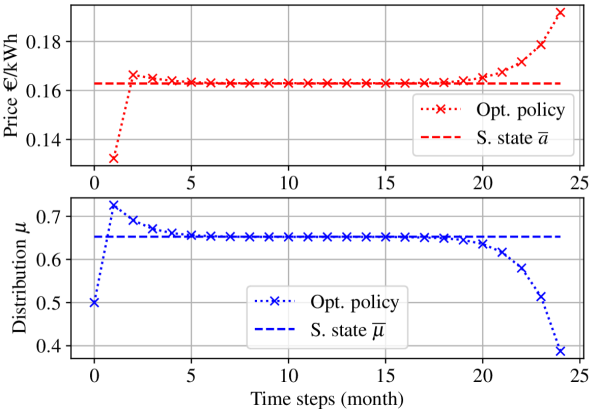
(a) Optimal finite horizon trajectory (provider action and customer distribution) for low switching cost.

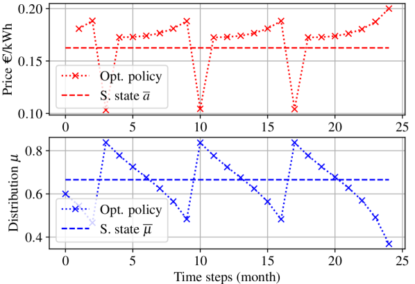
(b) Optimal finite horizon trajectory (provider action and customer distribution) for high switching cost.

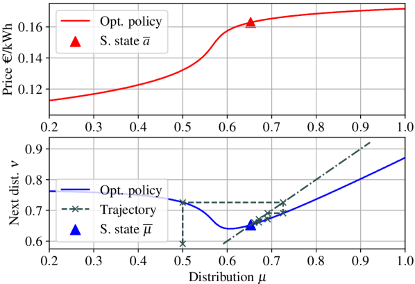
(c) Optimal decision for the long-run average reward (provider action and next customer distribution) for low switching cost. Graphical iteration is drawn in dotted lines.

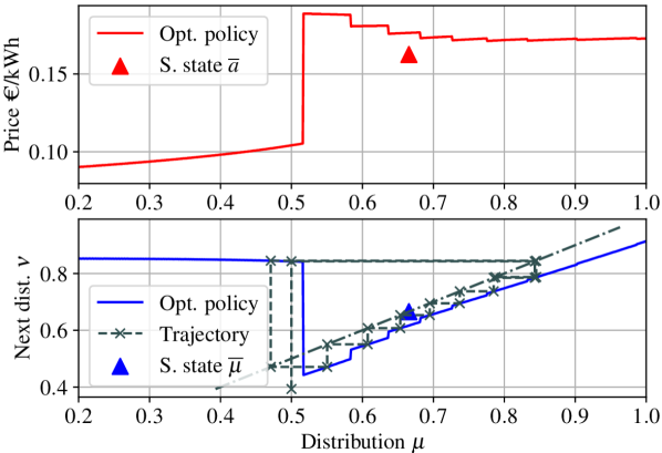
(d) Optimal decision for the long-run average reward (provider action and next customer distribution) for high switching cost. Graphical iteration is drawn in dotted lines.

Figure 2: Numerical results for both the finite horizon and long-term average reward criteria.
Low (resp. high) switching cost stands for $\gamma=20$ (resp. $25$).

VI CONCLUSION

We developed an ergodic control model to represent the evolution of a large population of customers, able to actualize their choices at any time. Using qualitative properties of the population dynamics (contraction in Hilbert’s projective metric), we showed the existence of a solution to the ergodic eigenproblem, which we applied to a problem of electricity pricing. A numerical study reveals the existence of optimal cyclic promotion mechanisms, that have already been observed in economics. We also quantified the suboptimality of constant-price strategy in terms of a specific duality gap.

The present model has connections with partially observable MDPs, in which the state space is also a simplex. We plan to explore such connections in future work. Besides, the convergence of the solution of the discretized ergodic equation (associated to the grid $\Sigma$) to the continuous solution will also be studied.

VII ACKNOWLEDGMENTS

We would like to thank the reviewers for their valuable and detailed comments, which help us to improve the clarity of this work.

VIII APPENDIX

VIII-A Proof materials

Lemma VIII.1

Let $\operatorname{\mathcal{D}}\subset\operatorname*{relint}(\Delta_{n})$, $n\in\operatorname{\mathbb{N}}$ and $x,y\in\operatorname{\mathcal{D}}$. Then,

$$n\left\|x-y\right\|_{\infty}\leq d_{H}(x,y)\Upsilon(\operatorname{Diam}_{H}(\operatorname{\mathcal{D}}))$$ (13)

where $\Upsilon(d)=\frac{1}{d}e^{d}(e^{d}-1)$.

Proof:

We use the results in [31]: Lemma 2.3 shows that for any vectors $u,x,y\in\operatorname{\mathcal{D}}$ such that there exist $a,b>0$ satisfying $ax\leq u\leq bx$ and $ay\leq u\leq by$, we have the following inequality:

$$\left\|x-y\right\|_{u}\leq\left(e^{d_{T}(x,y)}-1\right)e^{\max(d_{T}(x,u),d_{T}(y,u))}\enspace,$$

where $d_{T}$ denotes the Thompson distance, and $\left\|z\right\|_{u}=\inf\{a>0\mid-au\leq z\leq au\}$. In particular, by choosing $u=(1/n,\ldots 1/n)$ as the center of the simplex, $\left\|\cdot\right\|_{u}=n\left\|\cdot\right\|_{\infty}$. Moreover, $d_{T}(\cdot,\cdot)\leq d_{H}(\cdot,\cdot)$ on $\operatorname*{relint}(\Delta_{N}^{K})$, see [31, Eq. 2.4]. Therefore,

$$n\left\|x-y\right\|_{\infty} \leq\left(e^{d_{H}(x,y)}-1\right)e^{\max(d_{H}(x,u),d_{H}(y,u))}$$

$$\leq\left(e^{d_{H}(x,y)}-1\right)e^{\operatorname{Diam}_{H}(\operatorname{\mathcal{D}})}\enspace.$$

We easily conclude using the fact that $f:x\mapsto e^{x}-1$ is a convex function, and so for all $0\leq x\leq\bar{x},\,f(x)\leq x\frac{e^{\bar{x}}-1}{\bar{x}}$.

∎

VIII-B Proof of Lemma II.1

The set $\{\mu^{k}Q^{k}_{L}(a_{:L})\mid(a_{:L},\mu^{k})\in\operatorname{\mathcal{A}}^{L}\times\Delta_{N}\}$ is compact, since $(a_{:L},\mu^{k})\mapsto\mu^{k}Q^{k}_{L}(a_{:L})$ is continuous and $\Delta_{N}$ and $\operatorname{\mathcal{A}}$ are both compact. Therefore, $\operatorname{\mathcal{D}}_{L}$ is compact as it is the convex hull of a compact set in finite dimension. Then, the positiveness of $Q^{k}_{L}$ implies that $\operatorname{\mathcal{D}}^{k}_{L}\subset\operatorname*{relint}(\Delta_{N})$. Moreover, by property of the semiflow, $\phi_{t}(a_{:t},\mu_{0})=\phi_{L}\left(a_{t-L+1:t},\phi_{t-L}(a_{:t-L},\mu_{0})\right)\in\operatorname{\mathcal{D}}_{L}$.

VIII-C Proof of Theorem II.2

We first make the proof under the stronger assumption (A2’), and then deduce the general result.

Let $V^{*}_{\alpha}$ be the infinite horizon discounted objective, defined as

$$V^{*}_{\alpha}(\mu_{0})=\sup_{\pi\in\Pi}\;\sum_{t\geq 1}\alpha^{t-1}r(\pi_{t}(\mu_{t}),\mu_{t})\enspace,$$

where $\alpha$ is the discount factor and $\mu_{0}$ is the initial distribution.

We first prove that $(V^{*}_{\alpha})_{\alpha\in(0,1)}$ is equi-Lipschitz on $\operatorname{\mathcal{D}}_{1}$ (Lipschitz of a constant independent of $\alpha$) : let $a$ be the sequence of actions derived from an $\epsilon$-optimal policy $\pi$ and initial condition $\mu_{0}\in\operatorname{\mathcal{D}}_{1}$. Then, for $\nu_{0}\in\operatorname{\mathcal{D}}_{1}$

$$V^{*}_{\alpha}(\mu_{0})-V^{*}_{\alpha}(\nu_{0})\leq\sum_{t\geq 1}\alpha^{t-1}\left[\begin{split}&r\left(a_{t},\phi_{t}(a_{:t},\mu_{0})\right)\\ &-r\left(a_{t},\phi_{t}(a_{:t},\nu_{0})\right)\end{split}\right]+\epsilon\enspace.$$

The total reward is $(NM_{r})$-Lipschitz for the infinite norm. Therefore, using Lemma VIII.1, $\mu\mapsto r(a,\mu)$ is Lipschitz of constant $M^{\operatorname{\mathcal{D}}}_{r}:=\frac{1}{K}M_{r}\Upsilon(\operatorname{Diam}_{H}(\operatorname{\mathcal{D}}_{1}))$ for the Hilbert metric. Hence,

$$V^{*}_{\alpha}(\mu_{0})-V^{*}_{\alpha}(\nu_{0}) \leq M^{\operatorname{\mathcal{D}}}_{r}\sum_{t\geq 1}\alpha^{t\scalebox{0.5}[1.0]{$-$}1}d_{H}(\phi_{t}(a_{:t},\mu_{0}),\phi_{t}(a_{:t},\nu_{0}))$$

$$\quad+\epsilon\enspace.$$

From the Birkhoff theorem, one can derive that $d_{H}(\mu P(a),\nu P(a))\leq\kappa\,d_{H}(\mu,\nu)$ for $\mu,\nu\in\operatorname{\mathcal{D}}_{1},\,a\in\operatorname{\mathcal{A}}$, where $\kappa=\max_{a\in\operatorname{\mathcal{A}}}\kappa(P(a))<1$. As a consequence, $d_{H}(\phi_{t}(a_{:t},\mu_{0}),\phi_{t}(a_{:t},\nu_{0}))\leq\kappa^{t}d_{H}(\mu_{0},\nu_{0})$ and

$$V^{*}_{\alpha}(\mu_{0})-V^{*}_{\alpha}(\nu_{0})\leq M^{\operatorname{\mathcal{D}}}_{r}\sum_{t\geq 1}\alpha^{t-1}\kappa^{t}d_{H}(\mu^{0},\nu^{0})+\epsilon$$

$$\leq\frac{\kappa M^{\operatorname{\mathcal{D}}}_{r}}{1-\alpha\kappa}d_{H}(\mu^{0},\nu^{0})+\epsilon\leq\frac{\kappa M^{\operatorname{\mathcal{D}}}_{r}}{1-\kappa}d_{H}(\mu^{0},\nu^{0})+\epsilon\enspace.$$

The value function $V_{\alpha}^{*}$ is therefore $\left(\frac{\kappa M^{\operatorname{\mathcal{D}}}_{r}}{1-\kappa}\right)$-equi-Lipschitz for the Hilbert metric.

Let us define a reference distribution $\overline{\mu}\in\Delta_{N}^{K}$, $g^{*}_{\alpha}=(1-\alpha)V^{*}_{\alpha}(\overline{\mu})$, and $h^{*}_{\alpha}=V^{*}_{\alpha}-V^{*}_{\alpha}(\overline{\mu})\operatorname{1}_{\operatorname{\mathcal{D}}_{1}}$, then as $V^{*}_{\alpha}$ is equi-Lipschitz on $\operatorname{\mathcal{D}}_{1}$, $h^{*}_{\alpha}$ is equi-bounded and equi-Lipschitz on $\operatorname{\mathcal{D}}_{1}$ (in particular equi-continuous). By the Arzelà-Ascoli theorem, $h^{*}_{\alpha}\to h^{*}\in\operatorname{\mathcal{C}^{0}}(\operatorname{\mathcal{D}}_{1})$.

Finally, from the discounted reward approach, we get $\operatorname{\mathcal{B}}(\alpha V^{*}_{\alpha})=V^{*}_{\alpha}$, therefore

$$\frac{g^{*}_{\alpha}}{1-\alpha}\operatorname{1}_{\operatorname{\mathcal{D}}_{1}}+h^{*}_{\alpha}=\operatorname{\mathcal{B}}\left(\frac{\alpha g^{*}_{\alpha}}{1-\alpha}\operatorname{1}_{\operatorname{\mathcal{D}}_{1}}+\alpha h^{*}_{\alpha}\right)\enspace.$$

By the additive homogeneity property of the Bellman function, $g^{*}_{\alpha}\operatorname{1}_{\operatorname{\mathcal{D}}_{1}}+h^{*}_{\alpha}=\operatorname{\mathcal{B}}(\alpha h^{*}_{\alpha})\enspace.$ The fixed-point equation (6) is then obtained by continuity of the Bellman operator $\operatorname{\mathcal{B}}$.

To conclude, $h^{*}$ is convex since $V^{*}_{\alpha}$ is convex and the pointwise convergence preserves the convexity.

To deduce the general result with (A2), we define

• $\widetilde{\operatorname{\mathcal{A}}}:=\operatorname{\mathcal{A}}^{L}$, $\tilde{\alpha}:=\alpha^{L}$,

• $\tilde{\phi}_{\tau}(\tilde{a}_{:\tau},\mu_{0}):=\mu_{0}\prod_{1\leq t\leq\tau}Q(\tilde{a}_{t})$,

• $\tilde{r}(a_{:L},\mu):=\sum_{l\in[L]}\alpha^{l-1}r(a_{l},\phi_{l}(a_{:l},\mu))$,

• and $\tilde{\operatorname{\mathcal{B}}}:V\mapsto\max_{\tilde{a}\in\widetilde{\operatorname{\mathcal{A}}}}\{\tilde{r}(\tilde{a},\mu)+V(\nu)\mid\nu=\mu Q_{L}(\tilde{a})\}$.

and observe that

$$V_{\alpha}^{*}(\mu_{0})=\sum_{\tau\geq 1}\tilde{\alpha}^{\tau-1}\tilde{r}(\tilde{a}_{\tau},\tilde{\phi}_{\tau}(\tilde{a}_{:\tau},\mu_{0}))\enspace.$$

We have rescaled the time ($\tau$ instead of $t$) so that the transition matrix between time $\tau$ and time $\tau+1$ is $Q_{L}(\tilde{a}_{\tau})$. One $\tau$-time step corresponds to $L$ $t$-time steps. As the transition $Q_{L}(\tilde{a})$ is now positive, the proof is exactly the same as before, in the $\tau$-time space. We end up with the existence of $\tilde{h}\in\operatorname*{Lip}(\operatorname{\mathcal{D}}_{L})\cap\operatorname*{Vex}(\operatorname{\mathcal{D}}_{L})$ and $\tilde{g}^{*}\in\operatorname{\mathbb{R}}$ such that

$$\tilde{h}^{*}+\tilde{g}^{*}=\tilde{\operatorname{\mathcal{B}}}\tilde{h}^{*}\enspace.$$

Defining $g^{*}=\tilde{g}^{*}/L$, considering

$$h^{*}=\tilde{h}^{*} \vee\left(\operatorname{\mathcal{B}}\tilde{h}^{*}-g^{*}\operatorname{1}_{\operatorname{\mathcal{D}}_{L}}\right)\vee\left((\operatorname{\mathcal{B}})^{2}\tilde{h}^{*}-2g^{*}\operatorname{1}_{\operatorname{\mathcal{D}}_{L}}\right)$$

$$\vee\ldots\vee\left((\operatorname{\mathcal{B}})^{L-1}\tilde{h}^{*}-(L-1)g^{*}\operatorname{1}_{\operatorname{\mathcal{D}}_{L}}\right)\enspace,$$

and using the fact that the Bellman operator $\mathcal{B}$ commutes with the supremum operation, we get that $(g^{*},h^{*})$ satisfy (6) and $h^{*}\in\operatorname*{Lip}(\operatorname{\mathcal{D}}_{L})\cap\operatorname*{Vex}(\operatorname{\mathcal{D}}_{L})$.

VIII-D Proof of Proposition II.3

Let $\pi\in\Pi$ be a policy. By definition, for every $t$, $\operatorname{\mathcal{B}}^{\pi_{t}}h^{*}\leq\operatorname{\mathcal{B}}h^{*}=h^{*}+g^{*}\operatorname{1}_{\operatorname{\mathcal{D}}_{L}}$. Therefore, iterating the Kolmogorov operator, we obtain

$$(\operatorname{\mathcal{B}}^{\pi_{1}}\circ\ldots\circ\operatorname{\mathcal{B}}^{\pi_{t}})h^{*}\leq h^{*}+tg^{*}\operatorname{1}_{\operatorname{\mathcal{D}}_{L}}\enspace.$$

Let $\underline{h}^{*}:=\min_{\mu\in\operatorname{\mathcal{D}}_{L}}h^{*}(\mu)$ be the minimum of $h^{*}$. Then, $0_{\operatorname{\mathcal{D}}_{L}}\leq h-\underline{h}^{*}\operatorname{1}_{\operatorname{\mathcal{D}}_{L}}$, and so $(\operatorname{\mathcal{B}}^{\pi_{1}}\circ\ldots\circ\operatorname{\mathcal{B}}^{\pi_{t}})(0_{\operatorname{\mathcal{D}}_{L}})\leq h^{*}+(tg^{*}-\underline{h}^{*})\operatorname{1}_{\operatorname{\mathcal{D}}_{L}}\enspace.$ Finally,

$$\liminf_{t\to\infty}\frac{1}{t}(\operatorname{\mathcal{B}}^{\pi_{1}}\circ\ldots\circ\operatorname{\mathcal{B}}^{\pi_{t}})(0_{\operatorname{\mathcal{D}}_{L}})(\mu_{0})\leq g^{*}\enspace.$$

Any strategy has an average reward lower than $g^{*}$. As we have proved that the bias function $h^{*}$ is continuous on $\operatorname{\mathcal{D}}_{L}$, a maximizer $a^{*}(\mu)$ can be found for any state $\mu$, and so playing the strategy $a^{*}(\mu)$ achieves the best possible average gain $g^{*}$.

VIII-E Proof of Proposition III.3

First, from the geometrical convergence the dynamic (see Section VIII-D), the valid strategy consisting in executing action $\overline{a}$ each period of time induces an average reward of $\overline{g}$, regardless the initial distribution. Therefore, $\overline{g}\leq g^{*}$.

Then, for $\epsilon>0$, there exists $\lambda^{\epsilon}$ such that for any $(a,\mu)\in\operatorname{\mathcal{A}}\times\Delta_{N}^{k}$,

$$r(a,\mu P(a))+\left<\lambda^{\epsilon},\varphi(\mu P(a))-\varphi(\mu)\right>_{KN}\leq g^{(\varphi)}+\epsilon\enspace.$$

We construct a sequence of decision $a_{1},\ldots,a_{T}$ leading to distribution $\mu_{1},\ldots,\mu_{T}$. Then, at each period $t$,

$$r(a_{t},\mu_{t})+\left<\lambda^{\epsilon},\varphi(\mu_{t})-\varphi(\mu_{t-1})\right>_{KN}\leq g^{(\varphi)}+\epsilon\enspace.$$

Therefore, we take the mean over $t=1,\ldots,T$ to recover the average reward criteria:

$$\frac{1}{T}\sum_{t=1}^{T}r(a_{t},\mu_{t})+\frac{1}{T}\left<\lambda^{\epsilon},\varphi(\mu_{T})-\varphi(\mu_{0})\right>_{KN}\leq g^{(\varphi)}+\epsilon\enspace.$$

The second term converges to zero when $T\to\infty$ as we suppose that $\varphi$ is bounded on the simplex. So,

$$\liminf_{T\to\infty}\frac{1}{T}\sum_{t=1}^{T}r(a_{t},\mu_{t})\leq g^{(\varphi)}+\epsilon\enspace.$$

The latter inequality is valid for any $\epsilon>0$, and any sequence of action $(a_{t})_{t\in\operatorname{\mathbb{N}}}$, so $g^{*}\leq g^{(\varphi)}$.

VIII-F Proof of Theorem IV.1

In the proof, we forget the dependence on $k$ and $a$. The stationary probability is defined as $\forall m\in[N],\,\mu^{m}\left[1-P^{mm}\right]=\sum_{n\neq m}\mu^{n}P^{nm}\enspace.$ We can then replace by the definition of the probabilities (9) to obtain

$$\mu^{m}\left[\frac{\sum_{l\neq m}e^{\beta U^{m}}}{\sum_{l}e^{\beta[U^{l}+\operatorname{1}_{l=m}\gamma^{m}]}}\right]=\sum_{n\neq m}\mu^{n}\left[\frac{e^{\beta U^{m}}}{\sum_{l}e^{\beta[U^{l}+\operatorname{1}_{l=n}\gamma^{n}]}}\right]\enspace.$$

Defining $\tilde{\mu}^{n}:=\frac{\mu^{n}}{\sum_{l}e^{\beta[U^{l}+\operatorname{1}_{l=n}\gamma^{n}]}},$ we obtain

$$\forall m\in[N],\,\tilde{\mu}^{m}\sum_{l\neq m}e^{\beta U^{l}}=e^{\beta U^{m}}\sum_{l\neq m}\tilde{\mu}^{l}\enspace.$$

The solution $\tilde{\mu}^{n}:=\lambda e^{\beta U^{n}},n\in[N]$ is then a valid solution, and the constant $\lambda$ is chosen so that $\sum_{l\in[N]}\mu^{l}=1$:

$$\overline{\mu}^{kn}(a) =\lambda e^{\beta U^{kn}(a)}\sum_{m\in[N]}e^{\beta[U^{kn}(a)+\operatorname{1}_{m=n}\gamma^{kn}]}$$ (14)

$$\lambda^{-1} =\sum_{n\in[N]}e^{\beta U^{kn}(a)}\sum_{m\in[N]}e^{\beta[U^{km}(a)+\operatorname{1}_{m=n}\gamma^{kn}]}$$

Finally, $\eta^{kn}=\sum_{l}e^{\beta[U^{kl}+\operatorname{1}_{l=n}\gamma^{kn}]}/\sum_{l}e^{\beta U^{kl}}$. We recover the definition of $\overline{\mu}$ (14).

References

- [1] Ali Hortaçsu, Seyed Ali Madanizadeh and Steven L. Puller “Power to Choose? An Analysis of Consumer Inertia in the Residential Electricity Market” In American Economic Journal: Economic Policy 9.4 American Economic Association, 2017, pp. 192–226 DOI: 10.1257/pol.20150235
- [2] Tom Ndebele, Dan Marsh and Riccardo Scarpa “Consumer switching in retail electricity markets: Is price all that matters?” In Energy Economics 83 Elsevier BV, 2019, pp. 88–103 DOI: 10.1016/j.eneco.2019.06.012
- [3] Luisa Dressler and Stefan Weiergraber “Alert the inert! switching costs and limited awareness in retail electricity markets” In Unpublished manuscript, 2019
- [4] Luıs Cabral “Small switching costs lead to lower prices” In Journal of Marketing Research 46.4, 2009, pp. 449–451
- [5] Dan Horsky and Polykarpos Pavlidis “Brand Loyalty Induced Price Promotions: An Empirical Investigation” In SSRN Electronic Journal Elsevier BV, 2010 DOI: 10.2139/ssrn.1674765
- [6] William J. Allender and Timothy J. Richards “Brand Loyalty and Price Promotion Strategies: An Empirical Analysis” In Journal of Retailing 88.3 Elsevier BV, 2012, pp. 323–342 DOI: 10.1016/j.jretai.2012.01.001
- [7] James Flynn “Steady State Policies for Deterministic Dynamic Programs” In SIAM Journal on Applied Mathematics 37.1 Society for Industrial & Applied Mathematics (SIAM), 1979, pp. 128–147 DOI: 10.1137/0137009
- [8] Jean-Pierre Dubé, Günter J. Hitsch and Peter E. Rossi “Do Switching Costs Make Markets Less Competitive?” In Journal of Marketing Research 46.4 SAGE Publications, 2009, pp. 435–445 DOI: 10.1509/jmkr.46.4.435
- [9] Polykarpos Pavlidis and Paul B. Ellickson “Implications of parent brand inertia for multiproduct pricing” In Quantitative Marketing and Economics 15.4 Springer ScienceBusiness Media LLC, 2017, pp. 369–407 DOI: 10.1007/s11129-017-9187-8
- [10] Nicolas Gast and Bruno Gaujal “A mean field approach for optimization in discrete time” In Discrete Event Dynamic Systems 21.1 Springer ScienceBusiness Media LLC, 2010, pp. 63–101 DOI: 10.1007/s10626-010-0094-3
- [11] Médéric Motte and Huyên Pham “Mean-field Markov decision processes with common noise and open-loop controls” arXiv, 2019 DOI: 10.48550/ARXIV.1912.07883
- [12] Nicole Bäuerle “Mean Field Markov Decision Processes” arXiv, 2021 DOI: 10.48550/ARXIV.2106.08755
- [13] Anup Biswas “Mean Field Games with Ergodic cost for Discrete Time Markov Processes” arXiv, 2015 DOI: 10.48550/ARXIV.1510.08968
- [14] Onésimo Hernández-Lerma and Jean Bernard Lasserre “Discrete-Time Markov Control Processes” Springer New York, 1996 DOI: 10.1007/978-1-4612-0729-0
- [15] Vassili N. Kolokoltsov and Victor P. Maslov “Idempotent analysis and its applications” 401, Mathematics and its Applications Dordrecht: Kluwer Academic Publishers Group, 1997, pp. xii+305
- [16] Albert Fathi “The weak-KAM theorem in Lagrangian dynamics” Book to appear, 2022
- [17] Eduardo Garibaldi and Philippe Thieullen “Minimizing orbits in the discrete Aubry–Mather model” In Nonlinearity 24, 2011, pp. 563–611
- [18] John Mallet-Paret and Robert Nussbaum “Eigenvalues for a Class of Homogeneous Cone Maps Arising from Max-Plus Operators” In Discrete and Continuous Dynamical Systems 8.3, 2002, pp. 519–562
- [19] Marianne Akian, Stéphane Gaubert and Robert Nussbaum “A Collatz-Wielandt characterization of the spectral radius of order-preserving homogeneous maps on cones”, 2011 eprint: 1112.5968
- [20] Vincent Calvez, Pierre Gabriel and Stéphane Gaubert “Non-linear eigenvalue problems arising from growth maximization of positive linear dynamical systems” In Proceedings of the 53rd IEEE Annual Conference on Decision and Control (CDC), Los Angeles, 2014, pp. 1600–1607
- [21] Bas Lemmens and Roger Nussbaum “Nonlinear Perron–Frobenius Theory” Cambridge University Press, 2009 DOI: 10.1017/cbo9781139026079
- [22] Abraham Berman and Robert J. Plemmons “Nonnegative Matrices in the Mathematical Sciences” Society for IndustrialApplied Mathematics, 1994 DOI: 10.1137/1.9781611971262
- [23] Stéphane Gaubert “On the burnside problem for semigroups of matrices in the (max, +) algebra” In Semigroup Forum 52.1 Springer ScienceBusiness Media LLC, 1996, pp. 271–292 DOI: 10.1007/bf02574104
- [24] Martin L. Puterman “Markov Decision Processes” Wiley, 1994 DOI: 10.1002/9780470316887
- [25] Kenneth Train “Discrete Choice Methods with Simulation” Cambridge University Press, 2009 URL: https://EconPapers.repec.org/RePEc:cup:cbooks:9780521766555
- [26] Dimitri P. Bertsekas “A New Value Iteration method for the Average Cost Dynamic Programming Problem” In SIAM Journal on Control and Optimization 36.2 Society for Industrial & Applied Mathematics (SIAM), 1998, pp. 742–759 DOI: 10.1137/s0363012995291609
- [27] Milos Hauskrecht “Value-Function Approximations for Partially Observable Markov Decision Processes” In Journal of Artificial Intelligence Research 13 AI Access Foundation, 2000, pp. 33–94 DOI: 10.1613/jair.678
- [28] William S. Lovejoy “Computationally Feasible Bounds for Partially Observed Markov Decision Processes” In Operations Research 39.1 Institute for Operations Researchthe Management Sciences (INFORMS), 1991, pp. 162–175 DOI: 10.1287/opre.39.1.162
- [29] Stéphane Gaubert and Nikolas Stott “A convergent hierarchy of non-linear eigenproblems to compute the joint spectral radius of nonnegative matrices” In Mathematical Control & Related Fields 10.3 American Institute of Mathematical Sciences (AIMS), 2020, pp. 573–590 DOI: 10.3934/mcrf.2020011
- [30] Tobias Damm, Lars Grüne, Marleen Stieler and Karl Worthmann “An Exponential Turnpike Theorem for Dissipative Discrete Time Optimal Control Problems” In SIAM Journal on Control and Optimization 52.3 Society for Industrial & Applied Mathematics (SIAM), 2014, pp. 1935–1957 DOI: 10.1137/120888934
- [31] Marianne Akian, Stéphane Gaubert and Roger Nussbaum “Uniqueness of the fixed point of nonexpansive semidifferentiable maps” In Transactions of the American Mathematical Society 368.2 American Mathematical Society (AMS), 2015, pp. 1271–1320 DOI: 10.1090/s0002-9947-2015-06413-7