Construction of Machine-Learning Interatomic Potential Under Heat Flux Regularization and Its Application to Power Spectrum Analysis for Silver Chalcogenides

Abstract

We propose a data-driven approach for constructing machine-learning interatomic potentials (MLIPs) trained under a regularization with the aim of avoiding nonphysical heat flux. Specifically, we introduce a regularization term for the heat flux into the cost function of MLIPs to be minimized. Since the treatment of heat flux using MLIPs with regularization can be decomposed into elemental contributions or conducted in frequency space, this approach is expected to be useful for investigating the origin of thermal conductivity obtained from the Green-Kubo formula. However, the strength of regularization needs to be appropriately set because it may reduce not only the nonphysical part but also the intrinsic heat flux one. To this end, we investigated the conditions for constructing MLIPs that can reproduce the power spectra of heat flux associated with the empirical interatomic potential of Ag₂Se, which consists of pairwise functions and do not contain a nonphysical heat flux. The appropriate strength could be estimated from the variation of the magnitude of regularization term as well as root mean square errors for total potential energy, atomic force, and virial stress with respect to the strengths, without reference spectrum data. As an application example, we explored the differences in power spectra between superionic and nonsuperionic conducting phases based on the heat flux regularization to MLIPs trained with the first-principles calculation data of Ag₂S. Furthermore, our results demonstrate that training with the regularization improves the robustness of MLIPs as well as the reduction of the nonphysical heat flux.

I Introduction

The Green-Kubo (GK) method is an efficient tool for calculating thermal conductivity (TC) Volz and Chen (2000); Kubo (1957); Green (1952) and can be applied to irregular systems, where the heat flux ${\bf{J}}_{Q}$ sampled using a molecular dynamics (MD) simulation is used:

$$\kappa = \frac{1}{3k_{\rm B}T^{2}\varOmega}\int^{\infty}_{0}\langle{\bf{J}}_{Q}(t)\cdot{\bf{J}}_{Q}(0)\rangle dt,$$ ( I.1)

where $k_{\rm B}$, $T$, and $\varOmega$ are the Boltzmann constant, temperature, and volume of the supercell, respectively. The GK method has recently been combined with machine-learning interatomic potentials Morawietz and Artrith (2021) (MLIPs) to estimate the TCs of various materials. Tisi et al. (2021); Fan et al. (2021); Verdi et al. (2021); Li et al. (2020); Huang et al. (2019); Bosoni et al. (2019) MLIPs, which are trained with data obtained from first-principles molecular dynamics (FPMD) simulations, successfully replicate the high accuracy of FPMD while maintaining the low computational cost associated with conventional empirical interatomic potentials (EIPs).

However, a critical problem accompanies the analysis of the origin of TC using the GK method with MLIPs. The MLIP is a many-body potential; thus, the total potential energy $E^{\rm MLIP}$ is defined as the sum of the individual atomic potential energies $\varepsilon^{\rm MLIP}_{i}$,

$$E^{\rm MLIP}=\sum^{N_{\rm atom}}_{i}\epsilon^{\rm MLIP}_{i},$$ ( I.2)

where $N_{\rm atom}$ denotes the number of atoms in the system. The set {$\varepsilon^{\rm MLIP}_{i}$} is indirectly determined through the training of $E^{\rm MLIP}$. There are infinite sets of {$\varepsilon^{\rm MLIP}_{i}$} that generate the same value of $E^{\rm MLIP}$, i.e., $\varepsilon^{\rm MLIP}_{i}$ has a gauge (called an atomic gauge). Kim and Kang (2021) Thus, trained MLIPs with different initial weight parameters are likely to give the same $E^{\rm MLIP}$, but the set {$\varepsilon^{\rm MLIP}_{i}$} can be different for each MLIP. According to Kim et al., Kim and Kang (2021) the value of ${\bf{J}}_{Q}$ obtained from the interatomic potentials defined by Eq. (I.2) can be divided into ${\bf{J}}^{\rm net}_{Q}$ and ${\bf{J}}^{\rm nPhys}_{Q}$ due to the $atomic$ $gauge$:

$${\bf{J}}_{Q}={\bf{J}}^{\rm net}_{Q}+{\bf{J}}^{\rm nPhys}_{Q}.$$ ( I.3)

Only the net heat flux ${\bf{J}}^{\rm net}_{Q}$ contributes to the TC. In contrast, it has been revealed that ${\bf{J}}^{\rm nPhys}_{Q}$ has no effect on the calculation of TC via Eq. (I.1) because it is the total derivative with respect to time. Kim and Kang (2021); Ercole et al. (2016) Accordingly, ${\bf{J}}^{\rm nPhys}_{Q}$ is a nonphysical heat flux. The analysis based on the decomposition of ${\bf{J}}_{Q}$ becomes meaningless because of the presence of ${\bf{J}}^{\rm nPhys}_{Q}$, whose values would be different for each MLIP. On the other hand, the EIPs that consist of only pairwise functions can define the atomic potential energy unambiguously, and it is therefore considered that the influence of ${\bf{J}}^{\rm nPhys}_{Q}$ can be avoided. Previous studies with such pairwise EIPs succeeded in detailed analyses of the TC by decomposing ${\bf{J}}_{Q}$ into elemental/atomic components Fujii et al. (2020); Ouyang et al. (2014) or in frequency space. Fujii et al. (2018); Zhou et al. (2015); Zhou and Hu (2015); Sääskilahti et al. (2014) The presence of ${\bf{J}}^{\rm nPhys}_{Q}$ prevents the application of these useful analytical techniques to MLIPs.

We propose a solution to this problem with a data-driven approach, which provides a way to prevent ${\bf{J}}^{\rm nPhys}_{Q}$ from playing a role. Specifically, a regularization term associated with ${\bf{J}}_{Q}$ is introduced into the cost function $C$ to be minimized during the training of MLIPs:

$$C=C_{\rm 0}+p_{J}|{\bf{J}}_{Q}|^{2},$$ ( I.4)

where $C_{\rm 0}$ denotes the cost function without the regularization. $C_{\rm 0}$ includes the loss functions for the total potential energy, atomic force, and virial stress in the training of MLIPs. Irie et al. (2021); Fan et al. (2021); Marques et al. (2019); Zhang et al. (2018); Novikov et al. (2021) The regularization term brings ${\bf{J}}_{Q}$ closer to 0 during training, thus reducing ${\bf{J}}^{\rm nPhys}_{Q}$. However, if the regularization is too strong, ${\bf{J}}^{\rm net}_{Q}$ is also impaired, substantially reducing the accuracy of the MLIP. Therefore, it is vital to adjust the coefficient $p_{J}$.

To verify the effectiveness of this approach to heat flux regularization, we used an EIP of Ag₂Se Rino et al. (1988) consisting of pairwise functions. The EIP of Ag₂Se is physically superior, being able to describe the phase transitions between the liquid, superionic ($\alpha$), and nonsuperionic ($\beta$) phases. Shimojo and Okazaki (1991); Rino et al. (1988) First, taking advantage of the low computational cost of EIPs, the heat flux autocorrelation functions (HFACFs) $\langle{\bf{J}}_{Q}(t)\cdot{\bf{J}}_{Q}(0)\rangle$ for $\beta$- and $\alpha$-Ag₂Se and the corresponding power spectra $S(\omega)$ based on the Wiener-Khintchine theorem were calculated and used as reference data. In addition to $S(\omega)$ being affected by ${\bf{J}}^{\rm nPhys}_{Q}$, which helps to verify the effect of regularization, $S(0)$ matches the TC, and $S(\omega)$ for $\omega>0$ represents the frequency distribution of phonons. Mahdizadeh and Goharshadi (2014); Zhang and Jiang (2013) Second, we investigated the condition of the coefficient $p_{J}$ of the regularization term under which the MLIPs trained with the EIP-MD data of $\beta$- and $\alpha$-Ag₂Se reproduced the reference power spectra. Next, as an application, the results of the previous step were used to construct MLIPs trained with FPMD data for the $\beta$ and $\alpha$ phases of Ag₂S. Finally, we analyzed the difference between the power spectra of the two phases. Notwithstanding the difference in the dynamics of the Ag atoms, the TCs of the two phases have been experimentally estimated as similar values of approximately 0.5 Wm^-1K^-1. Hirata et al. (2020); Matsunaga et al. (2021) An analysis of power spectra in frequency space would provide information on the characteristic phonon distributions in the two phases. The results of the above-mentioned procedures might facilitate the development of silver chalcogenides such as Ag₂Se and Ag₂S as thermoelectric materials and thermoelectric diode devices.

In this study, we adopted the artificial neural network (ANN) potential Artrith and Urban (2016); Irie et al. (2021) as the MLIP. We recently proposed a computational framework for calculating TC by the GK method using ANN potentials, reporting the possibility of estimating the TCs of $\beta$- and $\alpha$-Ag₂Se with high accuracy. Takeshita et al. (2022); Shimamura et al. (2021, 2020) In the present study, we further improved the framework by the heat flux regularization.

In section II, we explain our computational methodologies, such as the construction of the ANN potential, the formulas for the heat flux and the power spectrum, the creation of training data for Ag₂Se and Ag₂S, the cost function, the regularization term, and the calculation of TC and the power spectrum. In section III, we first discuss the estimation of the appropriate coefficient $p_{J}$ of the regularization term through the reproduction of power spectra from the EIP of Ag₂Se. Second, we apply this approach to Ag₂S without reference data and mention the difference between the power spectra of the $\beta$ and $\alpha$ phases. We finally present our conclusions in section IV.

II Computational Methods

II.1 ANN Potential

The ANN potentials considered in this study were constructed using the Aenet code, which is a training code developed by Artrith et al. Artrith and Urban (2016) The ANN potential constructed by the Aenet code comprised feed forward neural networks (FFNNs) created for each atomic species, comprising two hidden layers with ten nodes. The scaled hyperbolic tangent Artrith and Urban (2016) was used as the activation function of hidden layers. The total potential energy $E^{\rm ANN}$ is defined as the sum of the atomic potential energies {$\epsilon^{\rm ANN}_{i}$} output from FFNNs for all atoms in the system, Behler and Parrinello (2007) i.e., via Eq. (I.2).

A numerical descriptor $\sigma_{i}$ that characterizes the atomic structure around each atom was used as the input for the ANN potential to obtain $\epsilon^{\rm ANN}_{i}$. Among the various methods for creating such descriptors, Artrith et al. proposed the Chebyshev descriptor that exploits the recursivity of the Chebyshev polynomial. Artrith et al. (2017) The seventeen radial and five angular Chebyshev descriptors were used with the cutoff radii of 8 Å and 5 Å, respectively.

II.2 Green-Kubo method

II.2.1 Heat flux formula

The heat flux ${\bf{J}}_{Q}$ in Eq. (I.1) for the EIP of Ag₂Se and the ANN potential is defined as Shimamura et al. (2020)

$${\bf{J}}_{Q} = \sum^{N_{\rm atom}}_{i}(t_{i}+\epsilon_{i}){\bf{v}}_{i}\ +\sum^{N_{\rm atom}}_{i}{\rm W}_{i}{\bf{v}}_{i}$$ ( II.1)

$$- \sum^{2}_{\mu}h_{\mu}\sum^{N_{\mu}}_{i\in\mu}{\bf{v}}_{i}\ ,$$

where $t_{i}$, $\epsilon_{i}$, ${\bf{v}}_{i}$, and ${\rm W}_{i}$ are the kinetic energy, potential energy, velocity, and virial tensor for the $i$th atom, respectively. In addition, $h_{\mu}$ and $N_{\mu}$ denote the partial enthalpy and the number of atoms for the $\mu$th component in the system ($\mu\in$ {Ag, Se} for Ag₂Se and $\mu\in$ {Ag, S} for Ag₂S), respectively. The formulas for $\epsilon_{i}$ and ${\rm W}_{i}$ for the EIP of Ag₂Se are shown in Section I of the Supplementary Materials (SM). ${\rm W}_{i}$ for the ANN potential with the Chebyshev descriptor is defined as Shimamura et al. (2021)

$${\rm W}^{\rm ANN}_{i}=\sum_{j\neq i}{\bf{r}}_{ij}\otimes\frac{\partial\epsilon^{\rm ANN}_{j}}{\partial{\bf{r}}_{ji}},$$ ( II.2)

where ${\bf{r}}_{ij}$ $\equiv$ ${\bf{r}}_{j}-{\bf{r}}_{i}$ and ${\bf{r}}_{i}$ denotes $i$th atomic coordinate. Note that the summation of ${\rm W}_{i}$ over $N_{\rm atom}$ coincides with the total virial tensor ${\rm W}$ defined by the virial theorem. The potential part of the virial stress tensor ${\rm\Pi_{\rm pot}}$ is calculated by dividing ${\rm W}$ by the volume of the supercell $\varOmega$. The third term on the right-hand side in Eq. (II.1) is introduced to correct the difference in the particle number flux between each component, Perronace et al. (2002) which is necessary in binary or other multiple system.

In the GK method, decomposing ${\bf{J}}_{Q}$ into constituent parts enables us to estimate their respective contributions to the TC. To elucidate the elemental contributions from components 1 and 2 denoted as $\mu_{1}$ and $\mu_{2}$, respectively, ${\bf{J}}_{Q}$ in Eq. (II.1) is decomposed into ${\bf{J}}_{\mu 1}$ and ${\bf{J}}_{\mu 2}$. Incidentally, ${\bf{J}}_{Q}$ can be also divided into the kinetic (convective) and potential (conductive) parts denoted as ${\bf{J}}_{\rm K}$ and ${\bf{J}}_{\rm P}$, respectively. ${\bf{J}}_{\rm K}$ and ${\bf{J}}_{\rm P}$ consist of terms in Eq. (II.1) containing $t_{i}$ and $\epsilon_{i}$ and containing ${\rm W}_{i}$, respectively.

II.2.2 Power spectrum of heat flux

According to the Wiener-Khintchine theorem, the Fourier transformation of the time series of the HFACF produces the power spectrum $S(\omega)$:

$$S(\omega) = \int^{\infty}_{-\infty}e^{i\omega t}\langle{\bf{J}}_{Q}(t)\cdot{\bf{J}}_{Q}(0)\rangle dt$$ ( II.3)

$$= 2\int^{\infty}_{0}\cos(\omega t)\langle{\bf{J}}_{Q}(t)\cdot{\bf{J}}_{Q}(0)\rangle dt.$$

Furthermore, the elemental and kinetic/potential contributions of $S(\omega)$ can also be calculated using the decomposed heat fluxes mentioned in section II.2.1: $S(\omega)=S_{\mu 1\mathchar 45\relax\mu 1}(\omega)+S_{\mu 1\mathchar 45\relax\mu 2}(\omega)+S_{\mu 2\mathchar 45\relax\mu 1}(\omega)+S_{\mu 2\mathchar 45\relax\mu 2}(\omega)$ and $S(\omega)=S_{\rm K\mathchar 45\relax K}(\omega)+S_{\rm K\mathchar 45\relax P}(\omega)+S_{\rm P\mathchar 45\relax K}(\omega)+S_{\rm P\mathchar 45\relax P}(\omega)$.

II.3 Generation of Ag₂Se training data by MD simulation with EIP

The MD simulations in this paper were executed using the QXMD Shimojo et al. (2019) code. In this section, we use the EIP proposed by Rino et al., Rino et al. (1988) comprising three pairwise potential functions: repulsive, dielectric dipole interaction, and Coulomb interaction terms (see Section I of the SM).

II.3.1 $\beta$-Ag₂Se at 300 K

We generated the training data of $\beta$-Ag₂Se at 300 K by performing MD simulations with the EIP of Ag₂Se. Rino et al. (1988) The unit cell of $\beta$-Ag₂Se reproduced by the EIP has an orthorhombic structure consisting of four Ag₂Se molecules with the following lattice parameters: $a=4.29$ Å, $b=6.82$ Å, and $c=8.25$ Å. Shimojo and Okazaki (1991) Using the $8\times 2\times 2$ unit cell structure consisting of 256 Ag and 128 Se atoms under periodic boundary conditions, an MD simulation with the canonical ensemble Nosé (1984) (hereinafter called $NVT$-MD) was performed with 100,000 steps at 300 K. The time step $\Delta t$ was set to 2.42 fs. A total of 1,000 MD steps were used as training data by extracting every 100 steps from the 100,000 MD steps to remove similar structures. The atomic coordinates {${\bf{r}}^{\beta\rm EIP}_{I,i}$}, atomic velocities {${\bf{v}}^{\beta\rm EIP}_{I,i}$}, total potential energy $E^{\beta\rm EIP}_{I}$, atomic force {${\bf{F}}^{\beta\rm EIP}_{I,i}$}, virial tensor ${\rm W}^{\beta\rm EIP}_{I}$, and supercell volume $\varOmega^{\beta\rm EIP}_{I}$, were contained in the $I$th MD step data.

II.3.2 $\alpha$-Ag₂Se at 500 K

The data generated using the EIP of Ag₂Se in our previous study Shimamura et al. (2020) were used in this study. Using the experimentally obtained number density for $\alpha$-Ag₂Se at 500 K (0.0461 Å^-3), Okazaki (1967) we prepared a system with 256 Ag and 128 Se atoms in a cubic supercell under periodic boundary conditions. The length of one side of the supercell was 20.271 Å. For the configuration, an $NVT$-MD simulation using the EIP of Ag₂Se was performed with 100,000 steps at 500 K. The time step $\Delta t$ was set to 2.42 fs. A total of 1,000 MD steps were used as training data by extracting every 100 steps. The atomic coordinates {${\bf{r}}^{\alpha\rm EIP}_{I,i}$}, atomic velocities {${\bf{v}}^{\alpha\rm EIP}_{I,i}$}, total potential energy $E^{\alpha\rm EIP}_{I}$, atomic force {${\bf{F}}^{\alpha\rm EIP}_{I,i}$}, virial tensor ${\rm W}^{\alpha\rm EIP}_{I}$, and supercell volume $\varOmega^{\alpha\rm EIP}_{I}$, were contained in the $I$th MD step data.

II.4 Generation of training data of Ag₂S by FPMD simulation

II.4.1 $\beta$-Ag₂S at 300 K

We created training data of $\beta$-Ag₂S at 300 K by performing FPMD simulations. The electronic states were calculated by the projector augmented wave method Blöchl (1994); Kresse and Joubert (1999) within the framework of density functional theory (DFT). Hohenberg and Kohn (1964); Kohn and Sham (1965) Projector functions were generated for the 4$d$, 5$s$, and 5$p$ states of Ag and for the 3$s$, 3$p$, and 3$d$ states of S. The Perdew-Burke-Ernzerhof generalized gradient approximation Perdew et al. (1996) was employed for the exchange correlation energy. To correctly represent the electronic states in localized $d$ orbitals of Ag, the DFT+U method Anisimov et al. (1997) with the effective parameter for the Coulomb interaction $U_{\rm eff}=6.0$ eV Fukushima et al. (2019); Santamaría-Pérez et al. (2012) was used. The empirical correction of the van der Waals interaction by the DFT-D approach Grimme (2006) was employed. The plane wave cutoff energies were 20 and 200 Ry for the electronic pseudo-wave function and pseudo-charge density, respectively. The energy functional was minimized iteratively using a preconditioned conjugate-gradient method Shimojo et al. (2001). The $\Gamma$ point was used for Brillouin zone sampling.

The unit cell of $\beta$-Ag₂S has a monoclinic structure consisting of four Ag₂S groups with lattice parameters: $a=4.231$ Å, $b=6.930$ Å, $c=9.526$ Å, and $\beta=125.48^{\circ}$. Sadanaga and Sueno (1967) Considering that the structure is a slightly distorted bcc lattice of S atoms, 32 unit cells were arranged to construct an atomic configuration close to cubic structure, containing 256 Ag and 128 S atoms. The lattice parameters of supercell were $a=19.548$ Å, $b=19.052$ Å, $c=19.548$ Å, $\alpha=90.871^{\circ}$, $\beta=90.312^{\circ}$, and $\gamma=90.871^{\circ}$. Using the configuration under periodic boundary conditions, an FPMD simulation with the isothermal and isobaric ensemble (hereinafter called $NPT$-FPMD) was performed with 3,000 steps at 300 K and 0 GPa. The time step $\Delta t$ was set to 1.21 fs. A total of 1,000 MD steps were used as training data by extracting every 3 steps. The $I$th MD step data contained the atomic coordinates {${\bf{r}}^{\beta\rm FP}_{I,i}$}, atomic velocities {${\bf{v}}^{\beta\rm FP}_{I,i}$}, total potential energy $E^{\beta\rm FP}_{I}$, atomic force {${\bf{F}}^{\beta\rm FP}_{I,i}$}, virial tensor ${\rm W}^{\beta\rm FP}_{I}$, and supercell volume $\varOmega^{\beta\rm FP}_{I}$.

II.4.2 $\alpha$-Ag₂S at 600 K

We created training data of $\alpha$-Ag₂S at 600 K by performing FPMD simulations. The electronic state calculation was performed with the same setting as that for $\beta$-Ag₂S described in the previous section II.4.1. Using the experimental lattice constant of $\alpha$-Ag₂S, Sadovnikov et al. (2018) we prepared a system with 256 Ag and 128 S atoms in a cubic supercell under periodic boundary conditions, where the length of one side of the supercell was 19.496 Å.

With that configuration, an $NPT$-FPMD simulation was performed with 3,000 steps at 600 K and 0 GPa. The time step $\Delta t$ was set to 1.21 fs. A total of 1,000 MD steps were used as training data by extracting every 3 steps. The $I$th MD step data contained the atomic coordinates {${\bf{r}}^{\alpha\rm FP}_{I,i}$}, atomic velocities {${\bf{v}}^{\alpha\rm FP}_{I,i}$}, total potential energy $E^{\alpha\rm FP}_{I}$, atomic force {${\bf{F}}^{\alpha\rm FP}_{I,i}$}, virial tensor ${\rm W}^{\alpha\rm FP}_{I}$, and supercell volume $\varOmega^{\alpha\rm FP}_{I}$.

II.5 Training of ANN potential

II.5.1 Cost function

We define the following cost function $C$ for training ANN potentials. It comprises three loss functions associated with the total potential energy (first term), atomic force (second term), and virial (third term), and a regularization term associated with the heat flux (fourth term):

$$C = \frac{p_{E}}{2}\frac{1}{N_{I}}\sum^{N_{I}}_{I}\left(\frac{E^{\rm ANN}_{I}-E^{\rm Ref}_{I}}{N_{{\rm atom},I}}\right)^{2}$$ ( II.4)

$$+ \frac{p_{F}}{2}\frac{1}{N_{I}}\sum^{N_{I}}_{I}\frac{1}{3N_{{\rm atom},I}}\sum^{N_{{\rm atom},I}}_{i}\ \left({\bf{F}}^{\rm ANN}_{I,i}-{\bf{F}}^{\rm Ref}_{I,i}\right)^{2}$$

$$+ \frac{p_{W}}{2}\frac{1}{N_{I}}\sum^{N_{I}}_{I}\frac{1}{6}\sum^{6}_{j}\ \left(\frac{{W}^{\rm ANN}_{I,j}-{W}^{\rm Ref}_{I,j}}{N_{{\rm atom},I}}\right)^{2}$$

$$+ \frac{p_{J}}{2}\frac{1}{N_{I}}\sum^{N_{I}}_{I}\frac{1}{3N_{{\rm atom},I}}\left({\bf{J}^{\prime}}_{{Q},I}\right)^{2},$$

where $N_{I}$ denotes the number of training data and ${\bf{F}}^{\rm ANN}_{i}$ is given by Shimamura et al. (2021)

$${\bf{F}}^{\rm ANN}_{i} = \sum^{N_{\rm atom}}_{j}{\bf{F}}^{\rm ANN}_{ij}$$ ( II.5)

$$= -\sum^{N_{\rm atom}}_{j}\left[\frac{\partial\epsilon^{\rm ANN}_{i}}{\partial{\bf{r}}_{ji}}+\frac{\partial\epsilon^{\rm ANN}_{j}}{\partial{\bf{r}}_{ji}}\right].$$

The pairwise force ${\bf{F}}^{\rm ANN}_{ij}$ satisfies Newton’s third law. Fan et al. (2015) The prime heat flux ${\bf{J}^{\prime}}_{{Q}}$ in the fourth term of Eq. (II.4) will be described in the next section II.5.2. Because these terms differ in dimension and size, $p_{E}$, $p_{F}$, $p_{W}$, and $p_{J}$ are introduced as adjustable parameters. The symbols with “Ref” denote training data, i.e., those labeled “$\beta$EIP”, “$\alpha$EIP”, “$\beta$FP”, or “$\alpha$FP” and explained in sections II.3 and  II.4.

With each "Ref" data, we performed training on 80% of them and the remaining 20% were used for testing. Hereafter, the former and latter are called the Train and Test data sets, respectively. The Levenberg-Marquardt method Artrith and Urban (2016) was adopted for the optimization process. Further details of the training procedures undertaken to minimize the cost function are provided in Section II of the SM, except for $p_{J}$, whose values are presented in section II.5.2.

II.5.2 Regularization term of heat flux

The definition of ${\bf{J}^{\prime}}_{{Q}}$ in Eq. (II.4) is different from that of ${\bf{J}}_{{Q}}$ in Eq. (II.1):

$${\bf{J}^{\prime}}_{Q} = \sum^{N_{\rm atom}}_{i}{\rm W}^{\rm ANN}_{i}{\bf{u}}^{\rm Ref}_{i},$$ ( II.6)

where ${\bf{u}}^{\rm Ref}_{i}$ is a renormalized velocity of the $i$th atom calculated from the atomic velocities {${\bf{v}}^{\rm Ref}_{i}$} in the training data. If the $i$th atom belongs to the $\mu$th component, ${\bf{u}}^{\rm Ref}_{i}$ is calculated by subtracting the average velocity of all atoms belonging to the $\mu$th component from ${\bf{v}}^{\rm Ref}_{i}$:

$${\bf{u}}^{\rm Ref}_{i} = {\bf{v}}^{\rm Ref}_{i}-\frac{1}{N_{\mu}}\sum^{N_{\mu}}_{j\in\mu}{\bf{v}}^{\rm Ref}_{j}.$$ ( II.7)

The reason for using the renormalized velocity is to play an alternative role to the third term of Eq. (II.1). Marcolongo et al. recently showed that replacing atomic velocities in the heat flux formula with the renormalized velocities approximately corresponds to the introduction of the correction embodied in the third term. Marcolongo et al. (2020) Since the calculation of enthalpy requires a huge number of statistics and obtaining it from a small amount of training data causes an error in the calculation of heat flux, their approach was employed in the regularization term. The reason for considering only the potential part of the heat flux in Eq. (II.6) was that its contribution to the TC was dominant compared to that of the kinetic part in our previous studies regarding silver chalcogenides. Takeshita et al. (2022); Shimamura et al. (2021)

The effect of the regularization term on training is controlled by the magnitude of its coefficient $p_{J}$. In this study, in addition to $p_{j}=0.0$, we mainly set $p_{J}=10^{\mathchar 45\relax 4}$, $10^{\mathchar 45\relax 3}$, $10^{\mathchar 45\relax 2}$, or $10^{\mathchar 45\relax 1}$ to construct ANN potentials and compare their results.

Furthermore, we defined the magnitude of the heat flux for regularization, $\Delta J_{Q}$, to evaluate the value of the heat flux in training as: $\Delta J_{Q}$ = $\sqrt{\frac{1}{N_{I}}\sum^{N_{I}}_{I}\frac{1}{3N_{{\rm atom},I}}\left({\bf{J}^{\prime}}_{{Q},I}\right)^{2}}$ (eV$\cdot$Å/ps).

II.6 Calculation of power spectrum of heat flux

In this study, the power spectra $S(\omega)$ for the following five potential models were computed:

1. EIP of Ag₂Se for creating reference data of $\beta$- and $\alpha$-Ag₂Se.

2. ANN potentials trained with EIP-MD data of $\beta$-Ag₂Se.

3. ANN potentials trained with EIP-MD data of $\alpha$-Ag₂Se.

4. ANN potentials trained with FPMD data of $\beta$-Ag₂S.

5. ANN potentials trained with FPMD data of $\alpha$-Ag₂S.

Using the same initial atomic configuration, temperature, and time step as those for the training data, an $NVT$-MD simulation was performed. Subsequently, a 1,000,000 MD-step simulation with the microcanonical ensemble (hereinafter called $NVE$-MD) was performed for sampling ${\bf{J}}_{Q}$ as defined in Eq. (II.1). The power spectra $S(\omega)$ were finally computed using Eq. (II.3) with an upper limit of integration of 2 ps.

As described in section I, ${\bf{J}}_{Q}$ for the ANN potential is considered to depend on its initial weight parameters. Therefore, for statistical evaluation, five ANN potentials with different initial weight parameters at each $p_{J}$ were constructed. These potentials are denoted as ANN1-ANN5 hereafter. The same initial values were used if the names of the potentials matched, even when the values of $p_{J}$ were different.

III Results and Discussion

III.1 The reference power spectrum data obtained with EIP of Ag₂Se

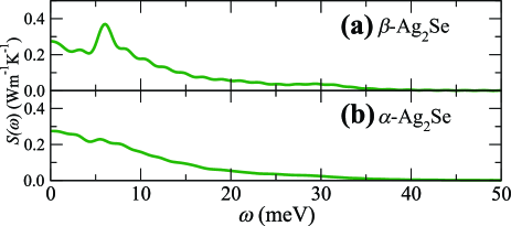
Figure 1: Power spectra of heat flux $S(\omega)$ obtained by the empirical interatomic potential (EIP) of Ag₂Se for (a) $\beta$- and (b) $\alpha$-Ag₂Se.

The power spectra $S(\omega)$ of $\beta$- and $\alpha$-Ag₂Se calculated using the EIP are displayed in Fig. 1. Although the obtained TCs are almost the same at $\sim$0.3 Wm^-1K^-1, the profiles are distinctly different. The power spectrum of the $\beta$ phase is characterized by a peak near 7 meV. This peak is due to the $S_{\rm Ag\mathchar 45\relax Ag}(\omega)$, as shown in Fig. S1 of the SM. The time variation of the corresponding HFACF and the cumulative TC $\kappa(t)$ defined in Eq. (III.1) are shown in Fig. S2 of the SM.

III.2 Results of ANN potentials trained with EIP-MD data

III.2.1 Power spectra of $\beta$-Ag₂Se and how to estimate the appropriate $p_{J}$

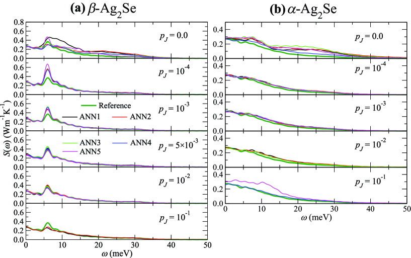
Figure 2: $S(\omega)$ obtained by the EIP of Ag₂Se (Reference, dark green) and trained ANN potentials with the heat flux regularization under each $p_{J}$ for (a) $\beta$- and (b) $\alpha$-Ag₂Se. ANN potentials (ANN1-ANN5) are trained with five different initial weight parameters (identified by colors in the figures above).

The dependence of the $\beta$-Ag₂Se power spectra on the regularization coefficient $p_{J}$ is shown in Fig. 2(a), where the results of five ANN potentials (ANN1-ANN5) with different initial weight parameters are included. The corresponding HFACFs and $\kappa(t)$ are shown in Figs. S3(a) and S3(c) of the SM. With $p_{J}$ = 0.0 (i.e., without the regularization), the values of the TCs are almost the same (at $\sim$0.3 Wm^-1K^-1) for the five ANN potentials, whereas the spectra differ. The profiles from 0 to 5 meV indicate that the power spectrum $S$($\omega$) of each of the ANN potentials lies close to the reference spectrum in this range; however, above 10 meV the match is poor. As mentioned in section I, this occurs because ${\bf{J}}^{\rm nPhys}_{Q}$ is different for each ANN potential. In contrast, with $p_{J}=10^{\mathchar 45\relax 4}$, $10^{\mathchar 45\relax 3}$, and $10^{\mathchar 45\relax 2}$, the power spectra show very similar profiles among all the ANN potentials, although the peak heights at 7 meV for 10^-4 and 10^-3 were not identical. The results with $p_{J}$ = 10^-2 were in good agreement with the reference spectrum for all five ANN potentials. This result implies that ${\bf{J}}^{\rm nPhys}_{Q}$ was successfully reduced by the heat flux regularization.

Training with a much stronger regularization (i.e., $p_{J}$ = $10^{\mathchar 45\relax 1}$) not only renders the power spectra incompatible with the reference spectrum (evidenced by the lower peak heights at 7 meV), but also makes it difficult to perform long-term MD simulations. Three of the five ANN potentials were unable to complete the 1,000,000-step $NVE$-MD simulations. Hence, the corresponding spectra derived from ANN3-ANN5 are not depicted in Fig. 2(a). The root mean square errors (RMSEs) for the total potential energy ($\Delta E$), atomic force ($\Delta F$), and virial stress from the contribution of the potential energy ($\Delta\varPi_{\rm pot}$), averaged over the five ANN potentials, are illustrated in Figs. 3(a)-3(c), as a function of $p_{J}$. The specific formulas for the RMSEs are provided in Section II C of the SM. The RMSEs for the Train and Test data are almost identical, suggesting that no overfitting occurs. In addition, the magnitude of the heat flux for regularization $\Delta J_{Q}$ obtained from the training is shown as a function of $p_{J}$ for $\beta$-Ag₂Se in Fig. 3(d). The averages and error bars (standard deviations) of the RMSEs for $p_{J}$ = $10^{\mathchar 45\relax 1}$ have much larger values compared to those for the other values of $p_{J}$, indicating that the accuracies of the ANN potentials worsened drastically as $p_{J}$ approached $10^{\mathchar 45\relax 1}$. Conversely, $\Delta J_{Q}$ was the smallest when $p_{J}$ = $10^{\mathchar 45\relax 1}$. We hypothesize that the effect of strong regularization on ${\bf{J}}^{\rm net}_{Q}$, the net heat flux part, reduced the robustness of the ANN potentials.

These results provide a foundation for finding the appropriate $p_{J}$ without resorting to reference data. $\Delta J_{Q}$ decreases monotonically as $p_{J}$ increases. This behavior was the opposite of trend displayed by the RMSEs. The optimal value of $p_{J}$ would achieve moderately low values for both $\Delta J_{Q}$ and the RMSEs. Note that stronger regularization results in a greater difference between the values of $\Delta J_{Q}$ obtained for the Train and Test data. This result may also be used to estimate the appropriate value of $p_{J}$ because the difference between the values of $\Delta J_{Q}$ for the Train and Test data is expected to increase when excessive regularization is imposed.

We sought an optimal value of $p_{J}$ for $\beta$-Ag₂Se as follows. As $\Delta E$ for the regularization with $p_{J}$ = 10^-2 is similar to that for $p_{J}$ = 10^-1 but relatively large compared to that of 10^-3, the optimum value for $p_{J}$ is inferred to lie below 10^-2. Therefore, we additionally trained ANN potentials with $p_{J}$ = 5$\times$10^-3. While $\Delta J_{Q}$ shows very little change for $p_{J}$ = 5$\times$10^-3 and 10^-2, the values of $\Delta E$, $\Delta F$, and $\Delta\varPi_{\rm pot}$ are all smaller for $p_{J}$ = 5$\times$10^-3 than for 10^-2; they also display power spectra close to the reference spectrum. In this way, we could determine an optimal value of $p_{J}$ by assessing the RMSEs and $\Delta J_{Q}$ as functions of $p_{J}$, even if there are no reference data. Although the RMSEs with $p_{J}$ = 5$\times$10^-3 were not minimal, we confirmed that the ANN potentials almost completely reproduced the atomic structure and ion dynamics, such as the radial distribution functions $g(r)$ and the mean squared displacements (MSDs) of the EIP of Ag₂Se, as shown in Figs. S4(a) and S5(a) of the SM.

III.2.2 Power spectra of $\alpha$-Ag₂Se

The power spectra of $\alpha$-Ag₂Se are shown in Fig. 2(b). The corresponding HFACFs and $\kappa(t)$ are shown in Figs. S3(b) and S3(d) of the SM. Qualitatively, the results are similar to those obtained for $\beta$-Ag₂Se as discussed in the previous section. With $p_{J}$ = 0.0, the power spectra for different ANN potentials were not consistent, as expected. All the spectra lay above the reference spectrum across the entire frequency range. Conversely, the training with $p_{J}$ = 10^-4 or 10^-3 generated improved spectra, in good agreement with the reference spectrum. With stronger regularization with $p_{J}$ = 10^-2 and 10^-1, $NVE$-MD simulations for 1,000,000 steps could be performed only with three (ANN1-ANN3) and two (ANN4 and ANN5) out of five ANN potentials, respectively. With reference to the RMSEs displayed in Figs. 3(e)-3(g), the accuracy of the ANN potentials became considerably poor from $p_{J}$ = 10^-3 to 10^-2. As shown in Fig. 3(h), the trend in $\Delta J_{Q}$ as a function of $p_{J}$ runs counter to that of the RMSEs. $\Delta J_{Q}$ for $p_{J}=$ 10^-2 shows a much larger deviation between the Train and Test data than for 10^-3, indicating that the strength of its regularization was excessive. The results discussed above imply that the optimal value for $\alpha$-Ag₂Se would be $p_{J}$ = 10^-3. The $g$($r$) and MSDs obtained from the ANN potentials are comparable to those of the EIP of Ag₂Se as shown in Figs. S4(b) and S5(b).

III.2.3 Improvement of robustness of ANN potential by heat flux regularization

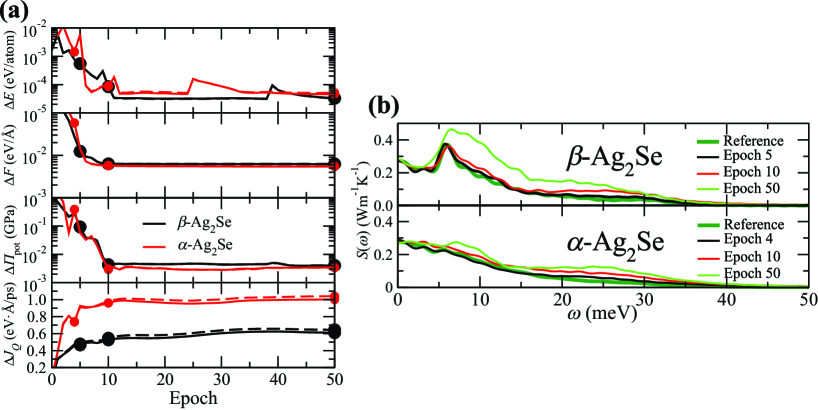
Figure 4: (a) The variation of $\Delta E$, $\Delta F$, $\Delta\varPi_{\rm pot}$, and $\Delta J_{Q}$ obtained during the training of an ANN potential for $\beta$- (black) and $\alpha$-Ag₂Se (red). The ANN potentials correspond to ANN1 for both phases in Fig. 2. The solid and dashed curves represent the RMSEs and $\Delta J_{Q}$ for the Train and Test data sets, respectively. (b) The corresponding $S(\omega)$ calculated using the ANN potentials at selected epochs marked with filled circles in (a), along with the results of the EIP of Ag₂Se (Reference). Epochs 4, 10, and 50 for $\beta$ and 5, 10, and 50 for $\alpha$ phases were selected.

Tracking the variation in the heat flux value of $\Delta J_{Q}$ during training reveals interesting behavior. The variations in $\Delta E$, $\Delta F$, $\Delta\varPi_{\rm pot}$, and $\Delta J_{Q}$ during training of one ANN potential (ANN1) without regularization for either $\beta$- or $\alpha$-Ag₂Se are illustrated in Fig. 4(a). Up to 10 epochs, for both phases, the RMSEs rapidly decrease whereas, conversely, the values of $\Delta J_{Q}$ increase. After 10 epochs, the values of $\Delta E$ and $\Delta\varPi_{\rm pot}$ tended to be slightly smaller but remain approximately constant, whereas the values of $\Delta J_{Q}$ display an increasing trend. The power spectra calculated using the ANN potentials at the selected three training epochs for each phase of Ag₂Se, i.e., 5, 10, and 50 epochs for the $\beta$ phase and 4, 10, and 50 epochs for the $\alpha$ phase are presented in Fig. 4(b). The power spectra for the $\beta$ and $\alpha$ phases at 5 and 4 epochs, respectively, were in good agreement with the reference spectra, but the deviation from the reference spectra increased with epoch number for both phases. The corresponding TC is almost unchanged (see the power spectra at $S(0)$). Therefore, it is considered that the small or nonexistent values of ${\bf{J}}^{\rm nPhys}_{Q}$ in the early epoch increased for subsequent epochs. The increasing trend of $\Delta J_{Q}$ seen in Fig. 4(a) would reflect the increase in the value of ${\bf{J}}^{\rm nPhys}_{Q}$. In addition, the RMSEs are higher at the epochs that give the agreement of the spectra with reference data. The robustness of the ANN potentials after 10 epochs, when the RMSEs are almost at their lowest, is expected to deteriorate because their heat fluxes include ${\bf{J}}^{\rm nPhys}_{Q}$.

The increase in ${\bf{J}}^{\rm nPhys}_{Q}$ is ascribed to the fact that $E^{\rm ANN}$, ${\bf F}^{\rm ANN}_{i}$, and W^ANN, that constitute the loss functions, are all sums of atomic components (i.e., $\varepsilon^{\rm ANN}_{i}$, ${\bf F}^{\rm ANN}_{ij}$, and W${}^{\rm ANN}_{i}$, respectively) and that there are no training constraints on these components. Because of the $atomic$ $gauge$ of $\varepsilon^{\rm ANN}_{i}$, Kim and Kang (2021) there are infinite sets of {$\varepsilon^{\rm ANN}_{i}$}, {${\bf F}^{\rm ANN}_{ij}$}, and {W${}^{\rm ANN}_{i}$} that produce the same values of $E^{\rm ANN}$, ${\bf F}^{\rm ANN}_{i}$, and W^ANN, respectively. During training, a set is sought for that will reduce the loss functions as much as possible, but the forcibly selected atomic components may have nonphysical values. It can be considered that either overfitting or underfitting of the atomic components occurred. Furthermore, the heat flux is also composed of these atomic components (see Eqs. (II.1) and (II.6)). ${\bf F}^{\rm ANN}_{ij}$, which contains the same derivatives of $\varepsilon^{\rm ANN}_{i}$ as W${}^{\rm ANN}_{i}$, would affect the heat flux indirectly through W${}^{\rm ANN}_{i}$ (see Eqs. (II.5) and (II.2)). Such a heat flux including nonphysical atomic components is considered to have a large ${\bf{J}}^{\rm nPhys}_{Q}$, which would be reflected in $\Delta J_{Q}$.

Therefore, it is expected that the heat flux regularization leads to converse behavior in the RMSEs and $\Delta J_{Q}$. In addition, since the regularization plays a role in suppressing the overfitting and underfitting of the atomic components, it improves the robustness of the ANN potentials. The above discussion also suggests that it is insufficient to measure the robustness of ANN potentials by the RMSEs alone. Minimizing the RMSEs does not necessarily mean constructing ANN potentials with high robustness because either overfitting or underfitting of the atomic components may have occurred. $\Delta J_{Q}$ should be used as an indicator of the robustness, in addition to the RMSEs.

III.3 Results of ANN potentials trained with FPMD data

The investigation using the EIP of Ag₂Se discussed in the previous section III.2 indicated the procedure for estimating an appropriate $p_{J}$ without reference data using the variations of the RMSEs and $\Delta J_{Q}$ with respect to $p_{J}$. This section applies the same approach to Ag₂S.

III.3.1 Power spectra of $\beta$- and $\alpha$-Ag₂S and the selection of appropriate $p_{J}$

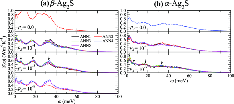
Figure 5: $S(\omega)$ obtained by the trained ANN potentials with heat flux regularization under each $p_{J}$ for (a) $\beta$- and (b) $\alpha$-Ag₂S. ANN potentials (ANN1-ANN5) are trained by five different initial weight parameters (identified by colors in the figures above). The black arrows in the power spectra for $p_{J}$ = 10^-3 indicate the peak positions of the $\beta$ phase, which are discussed in section III.3.2.

The power spectra for the ANN potentials for $\beta$- and $\alpha$-Ag₂S are shown in Figs. 5(a) and 5(b), respectively. The corresponding HFACFs and $\kappa(t)$ are shown in Fig. S6 of the SM. With $p_{J}$ = 0.0, only one ANN potential can perform stable $NVE$-MD simulations for 1,000,000 steps for each of $\beta$- and $\alpha$-Ag₂S. However, with $p_{J}$ = 10^-4 or 10^-3, stable simulations could be performed with almost all five ANN potentials. Only one ANN potential provided a failed simulation: ANN3 with $p_{J}=10^{\mathchar 45\relax 4}$ for $\alpha$ phase was failed. The different ANN potentials displayed very similar spectral profiles. These results show that heat flux regularization improved the robustness of the ANN potentials. However, with a larger $p_{J}$ = 10^-2, only three (ANN2, ANN4, and ANN5) and zero out of five ANN potentials provided stable MD simulations for $\beta$- and $\alpha$-Ag₂S, respectively.

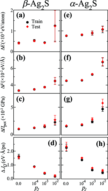
Figure 6: Averaged RMSEs and corresponding standard deviations (error bars) of $\Delta E$, $\Delta F$, and $\Delta\varPi_{\rm pot}$ over the five trained ANN potentials for (a-c) $\beta$- and (e-g) $\alpha$-Ag₂S. The values of $\Delta J_{Q}$ for (d) $\beta$- and (h) $\alpha$-Ag₂S are also shown. Black circles and red diamonds represent results obtained for the Train and Test data sets, respectively.

The RMSEs (i.e., $\Delta E$, $\Delta F$, and $\Delta\varPi_{\rm pot}$) of $\beta$- and $\alpha$-Ag₂S are shown in Figs. 6(a)-6(c) and 6(e)-6(g), respectively. In addition, the values of the magnitude of the heat flux for the regularization $\Delta J_{Q}$ for $\beta$ and $\alpha$ phases are shown in Figs. 6(d) and 6(h), respectively. In both phases, the averages and error bars of the RMSEs increased considerably as $p_{J}$ increased from 10^-3 to 10^-2. The values of $\Delta J_{Q}$ for $p_{J}$ = 10^-3 were substantially smaller than those for $p_{J}<10^{\mathchar 45\relax 3}$. $p_{J}$ = 10^-3 was therefore considered to be the most appropriate value for both phases. It was confirmed that the $g$($r$) and the MSDs obtained by the FPMD simulation and the ANN potentials trained with $p_{J}$ = 10^-3 coincided fairly well, as shown in Figs. S7 and S8 of the SM.

We hypothesize that the one reason of the difficulty of successfully performing long MD simulations of ANN potentials with $p_{J}$ = 0.0 for both $\beta$- and $\alpha$-Ag₂S is because of the large value of $\Delta J_{Q}$. The magnitudes with $p_{J}$ = 0.0 for both phases were much larger than those for the regularized trainings (i.e., $p_{J}$ > 0.0), suggesting that the ANN potentials provided larger values of ${\bf{J}}^{\rm nPhys}_{Q}$ as well. Therefore, the ANN potentials trained without regularization are considered to have undergone significant overfitting or underfitting of the atomic components (as explained in section III.2.3), making it difficult to predict accurate physical quantities; in particular, the atomic forces, thereby causing fatal computing errors to occur locally during MD simulations. Note that another reason could be attributed to the low diversity of training data. Because the FPMD training data were generated by a shorter simulation than the EIP-MD data, the diversity of atomic configurations included should be much lower. It was difficult to construct a robust ANN potential that could perform long-term MD simulations using such a low diversity data. Shimamura et al. (2019)

III.3.2 Power spectrum analysis for $\beta$ and $\alpha$ phases

We compared power spectra of $\beta$- and $\alpha$-Ag₂S for the most appropriate value $p_{J}=10^{\mathchar 45\relax 3}$, as shown in Fig. 5. The TCs of $\beta$- and $\alpha$-Ag₂S were 0.541 $\pm$ 0.030 and 0.516 $\pm$ 0.050 Wm^-1K^-1, respectively. These values are in close agreement with each other and with the experimental values. Hirata et al. (2020); Matsunaga et al. (2021)

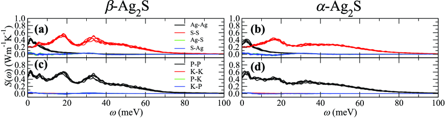
Figure 7: Decomposed $S(\omega)$ by (a-b) elemental contributions and (c-d) kinetic/potential parts obtained by the ANN potentials trained with the appropriate regularization for $\beta$- and $\alpha$-Ag₂S. The former is expressly $S$ = $S_{\rm Ag\mathchar 45\relax Ag}$ + $S_{\rm Se\mathchar 45\relax Se}$ + $S_{\rm Ag\mathchar 45\relax Se}$ + $S_{\rm Se\mathchar 45\relax Ag}$ and the latter $S$ = $S_{\rm P\mathchar 45\relax P}$ + $S_{\rm K\mathchar 45\relax K}$ + $S_{\rm P\mathchar 45\relax K}$ + $S_{\rm K\mathchar 45\relax P}$. For both $\beta$- and $\alpha$-Ag₂S, $p_{J}$ = 10^-3 is used for the regularization. For each decomposed $S(\omega)$, results obtained from the five ANN potentials trained with different initial weight parameters are shown.

However, the profiles of $S(\omega)$ show different features. The peaks at 6 and 34 meV present in the $\beta$-Ag₂S spectrum were no longer visible in the spectrum of $\alpha$-Ag₂S, and the height of the peak at 18 meV is lower in the latter spectrum. In contrast, $\alpha$-Ag₂S was found to have a heavier tailed distribution up to 90 meV. The components of the power spectra defined in section II.2.2 are displayed in Fig. 7. From the power spectra of the elemental contribution for $\beta$- and $\alpha$-Ag₂S shown in Figs. 7(a) and 7(b), respectively, the peaks at 6, 18, and 34 meV and the long tail of the spectra up to 90 meV are mainly attributed to $S_{\rm S\mathchar 45\relax S}(\omega)$. Conversely, the profiles of $S_{\rm Ag\mathchar 45\relax Ag}(\omega)$ and the cross terms ($S_{\rm Ag\mathchar 45\relax S}(\omega)$ and $S_{\rm S\mathchar 45\relax Ag}(\omega)$) did not display substantial variation between the $\beta$ and $\alpha$ phases. The peak at 3 meV resulted from $S_{\rm Ag\mathchar 45\relax Ag}(\omega)$ for both phases. From the power spectra of the kinetic/potential parts shown in Figs. 7(c) and  7(d), the potential part ($S_{\rm P\mathchar 45\relax P}(\omega)$) dominates the spectrum in both phases. The power spectrum describes the frequency distribution of phonons, and the intensity of its peak corresponds to the contribution of individual phonons. Mahdizadeh and Goharshadi (2014); Zhang and Jiang (2013) In addition, the phonon frequency analysis results for $\beta$-Ag₂S at 300 K using the Boltzmann transport equation Zhou et al. (2020) suggest that acoustic phonons predominantly contribute to the power spectrum up to $\sim$5 meV, while optical phonons predominantly contribute to the spectrum above that frequency. Considering these findings, our results for $\alpha$-Ag₂S suggest that instead of a decrease in optical phonons corresponding to the peaks at 6, 18, and 34 meV, high-frequency optical phonons with energies up to 90 meV appeared. The frequency ranges of the optical phonons due to the interactions between S atoms were different for $\beta$ and $\alpha$ phases. The heat flux regularization approach will allow us to access information about such phonon distributions that was previously unavailable in MLIPs.

IV Conclusion

In this paper, we proposed a data-driven approach to reduce the nonphysical heat flux (i.e., ${\bf{J}}^{\rm nPhys}_{Q}$) caused by the $atomic$ $gauge$ Kim and Kang (2021) by incorporating the regularization of the heat flux into the training of MLIPs. Because adjusting the strength of regularization is the key to achieving this reduction, we investigated the conditions for constructing MLIPs under which the power spectra of the heat flux of $\beta$- and $\alpha$-Ag₂Se calculated by the EIP of Ag₂Se could be reproduced. The EIP was composed of only pairwise functions where ${\bf{J}}^{\rm nPhys}_{Q}$ did not occur. The ANN potential was adopted as the MLIP in this study.

The strength of the effects could be controlled by the coefficient $p_{J}$. We found that the optimal value of $p_{J}$ could be estimated without access to reference spectra by clarifying the correlation of the RMSEs (i.e., $\Delta E$, $\Delta F$, and $\Delta\varPi_{\rm pot}$) and the magnitude of the heat flux for regularization (i.e., $\Delta J_{Q}$) with respect to $p_{J}$; that value of $p_{J}$ that minimizes both $\Delta J_{Q}$ and the RMSEs should be selected.

The heat flux regularization was applied to the ANN potentials trained with the FPMD data of $\beta$- and $\alpha$-Ag₂S. From their power spectra, the frequency ranges of optical phonons associated with due to the interactions between S atoms was found to be different in the two phases.

We also found that reducing ${\bf{J}}^{\rm nPhys}_{Q}$ through the regularization improved the robustness of the ANN potentials. This occurred because the regularization suppressed the overfitting and underfitting of the atomic components (i.e., $\varepsilon^{\rm ANN}_{i}$, ${\bf F}^{\rm ANN}_{ij}$, and W${}^{\rm ANN}_{i}$). We identified $\Delta J_{Q}$ as an useful indicator for measuring the robustness, in addition to the RMSEs.

With ANN potentials trained with the heat flux regularization, in future, we plan to investigate the composition dependence of the frequency distribution of phonons and the thermal conductivity of silver chalcogenide mixtures such as Ag₂S_1-xSe_x Matsunaga et al. (2021), using power spectrum analysis and effective analytical techniques Fujii et al. (2020, 2018); Zhou et al. (2015); Zhou and Hu (2015); Sääskilahti et al. (2014); Ouyang et al. (2014) based on the decomposition of heat flux.

Supplementary Material

See Supplemental Materials for detailed descriptions regarding the EIP of Ag₂Se (Section I), training of ANN potentials (Section II), and the definition of cumulative TC, $\kappa(t)$ (Section III). In Fig. S1, we show the decomposed power spectra according to their elemental contributions and kinetic/potential parts obtained by the EIP of Ag₂Se and ANN potentials trained with the appropriate regularization, for $\beta$- and $\alpha$-Ag₂Se. In Figs. S2, S3, S4, and S5, we show the HFACFs, $\kappa(t)$, $g(r)$, and MSDs obtained by the EIP of Ag₂Se and trained ANN potentials with the heat flux regularization under each $p_{J}$ for $\beta$- and $\alpha$-Ag₂Se. In Fig. S6, we show the HFACFs and $\kappa(t)$ obtained by trained ANN potentials with the regularization under each $p_{J}$, for $\beta$- and $\alpha$-Ag₂S. In addition, the $g(r)$ and the MSDs obtained by the FPMD simulation and the trained ANN potentials are shown in Figs. S7 and S8.

Data availavility

The data that support the findings of this study are available from the corresponding author upon reasonable request.

References

Figures

Figure 3: Averaged root mean square errors (RMSEs) and corresponding standard deviations (error bars) of the total potential energy ($\Delta E$), atomic force ($\Delta F$), and virial stress from the contribution of the potential energy ($\Delta\varPi_{\rm pot}$) over the five trained ANN potentials for (a-c) $\beta$- and (e-g) $\alpha$-Ag₂Se. The values of the magnitudes of heat flux for regularization ($\Delta J_{Q}$) for (d) $\beta$- and (h) $\alpha$-Ag₂Se are also shown. Black circles and red diamonds represent results obtained for the Train and Test data sets, respectively.

Supplementary Material for “Construction of Machine-Learning Interatomic Potential Under Heat Flux Regularization and Its Application to Power Spectrum Analysis for Silver Chalcogenides”

I Empirical Interatomic Potential of Ag₂Se and definition of its atomic potential, force, and virial tensor

The empirical interatomic potential $V^{\rm EIP}(r)$ for Ag₂Se proposed by Rino et al. Rino et al. (1988) is composed of three pairwise functions: repulsive, dielectric dipole interaction, and Coulomb interaction terms

$$V^{\rm EIP}\left(r\right)= \begin{cases}\frac{0.2408}{r^{11}}+\frac{0.2025}{r}&\left({\rm Ag\mathchar 45\relax Ag}\right)\\ \frac{86.6614}{r^{9}}-\frac{0.7088{\rm exp}(-r/4.43)}{r^{4}}-\frac{0.405}{r}&\left({\rm Ag\mathchar 45\relax Se}\right)\\ \frac{220.1905}{r^{7}}-\frac{5.67{\rm exp}(-r/4.43)}{r^{4}}+\frac{0.81}{r}&\left({\rm Se\mathchar 45\relax Se}\right)\end{cases},$$ ( I.1)

where the interatomic distance $r$ is measured in Å and the energies are given in units of ${e^{2}/}$Å = 14.389 eV. In addition, the functional form is defined for each component pair, i.e., Ag-Ag, Ag-Se, and Se-Se. For the empirical interatomic potential, atomic potential energy of the $i$th atom $\varepsilon^{\rm EIP}_{i}$ can be written as

$$\varepsilon^{\rm EIP}_{i}=\frac{1}{2}\sum_{j\neq i}V^{\rm EIP}(r_{ij}),$$ ( I.2)

where $r_{ij}$ $=$ $|{\bf{r}}_{ij}|$ $=$ $|{\bf{r}}_{j}-{\bf{r}}_{i}|$ denotes the interatomic distance between the $i$th and $j$th atoms. The summation $\sum^{N_{\rm atom}}_{i}\varepsilon^{\rm EIP}_{i}$ is equal to total potential energy $E^{\rm EIP}$. $N_{\rm atom}$ denotes the number of atoms in the system. Atomic virial tensor for the empirical interatomic potential ${\rm W}^{\rm EIP}_{i}$ is given by

$${\rm W}^{\rm EIP}_{i}=-\frac{1}{2}\sum_{j\neq i}{\bf{r}}_{ij}\otimes{\bf{F}}^{\rm EIP}_{ij},$$ ( I.3)

with ${\bf{F}}^{\rm EIP}_{ij}=\frac{\partial V^{\rm EIP}(r_{ij})}{\partial{\bf{r}}_{ij}}$, and the summation $\sum^{N_{\rm atom}}_{j}{\bf{F}}^{\rm EIP}_{ij}$ is equal to atomic force ${\bf{F}}^{\rm EIP}_{i}$. The sum of ${\rm W}^{\rm EIP}_{i}$ corresponds to the total virial tensor W^EIP.

$${\rm W}^{\rm EIP}=\sum^{N_{\rm atom}}_{i}{\rm W}^{\rm EIP}_{i}.$$ ( I.4)

II Training of ANN Potentials in this study

II.1 Training with Data Generated from Empirical Interatomic Potential of Ag₂Se

The total number of training data used for the cost function (Eq. (8) in the main text) reached $N_{I}\times(D_{\rm Energy}+D_{\rm Force}+D_{\rm Virial}+D_{\rm Velocity})=1000\times(1+3\times 384+6+3\times 384)=2311000$, where $N_{I}$ is the number of MD steps, and $D_{\rm Energy}$, $D_{\rm Force}$, $D_{\rm Virial}$, and $D_{\rm Velocity}$ are the dimensions of potential energy, atomic force, virial, and atomic velocity in one MD step data, respectively. Note that how to generate these data was explained in section II C in the main text.

The number of epochs was set to 50 for all training with data generated by the empirical interatomic potential (EIP) of Ag₂Se, and $p_{E}=p_{F}=1.0$ and $p_{W}=10^{\mathchar 45\relax 5}$ during the training. Please see section III B in the main text for the values of $p_{J}$ in each training.

II.2 Training with FPMD Data

The total number of training data used for the cost function (Eq. (8) in the main text) reached $N_{I}\times(D_{\rm Energy}+D_{\rm Force}+D_{\rm Virial}+D_{\rm Velocity})=1000\times(1+3\times 384+6+3\times 384)=2311000$. Note that how to generate these data was explained in section II D in the main text.

For all training with FPMD data, we took two-step scheme to train ANN potential efficiently by manipulating $p_{E}$, $p_{F}$, and $p_{W}$. $p_{F}$ was set to $1.0$ in both steps, while $p_{E}=10^{\mathchar 45\relax 3}$ and $p_{W}=10^{\mathchar 45\relax 6}$ in the first step and $p_{E}=10^{\mathchar 45\relax 1}$ and $p_{W}=10^{\mathchar 45\relax 1}$ in the second step. The number of epochs was set to 20 for each step. Adjusting the coefficients of the cost function during training in this way for efficiency has been actively carried out in previous studies Takeshita et al. (2022); Shimamura et al. (2021); Lee et al. (2020); Shimamura et al. (2019); Zhang et al. (2018). In addition, the two-step scheme adopted in this study above has been found to be capable of constructing highly accurate ANN potentials trained with Ag₂Se FPMD data Takeshita et al. (2022). Please see section III C in the main text for the values of $p_{J}$ in each training.

II.3 The formulas of root mean square errors

For total potential energy,

$$\Delta E = \sqrt{\frac{1}{N_{I}}\sum^{N_{I}}_{I}\left(\frac{E^{\rm ANN}_{I}-E^{\rm Ref}_{I}}{N_{{\rm atom},I}}\right)^{2}}.$$

For atomic force,

$$\Delta F = \sqrt{\frac{1}{N_{I}}\sum^{N_{I}}_{I}\frac{1}{3N_{{\rm atom},I}}\sum^{N_{{\rm atom},I}}_{i}\ \left({\bf{F}}^{\rm ANN}_{I,i}-{\bf{F}}^{\rm Ref}_{I,i}\right)^{2}}.$$

For virial stress from the contribution of the potential energy,

$$\Delta\varPi_{\rm pot} = \sqrt{\frac{1}{N_{I}}\sum^{N_{I}}_{I}\frac{1}{6\varOmega^{\rm Ref}_{I}}\sum^{6}_{j}\ \left({W}^{\rm ANN}_{I,j}-{W}^{\rm Ref}_{I,j}\right)^{2}}.$$

III Cumulative Thermal Conductivity

The cumulative thermal conductivity $\kappa(t)$ is calculated by

$$\kappa(t) = \frac{1}{3k_{\rm B}T^{2}\varOmega}\int^{t}_{0}\langle{\bf{J}}_{Q}(t^{\prime})\cdot{\bf{J}}_{Q}(0)\rangle dt^{\prime},$$ ( III.1)

where $k_{\rm B}$, $T$, $\varOmega$, and ${\bf{J}}_{Q}$ are Boltzmann constant, temperature, volume of supercell, and heat flux in Eq. (5) of the main text, respectively. In this study, $\kappa(t)$ were computed through Eq. (III.1) with the upper limit of integration of 2 ps. This is because $\kappa(t)$ converged well at 2 ps, as shown in Figs. S2, S3, and S6.

IV Supplementary Figures

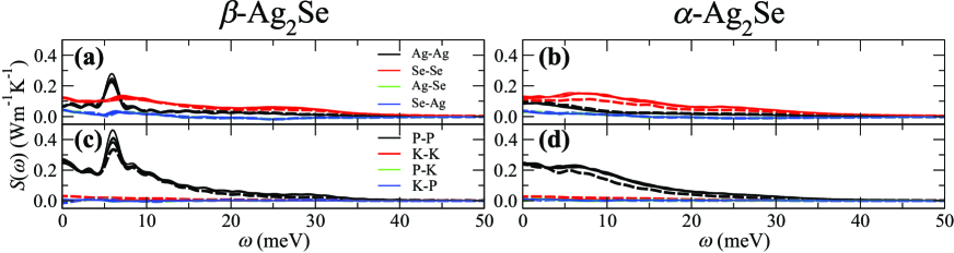
Figure S 1: Decomposed power spectra of heat flux $S(\omega)$ by (a-b) elemental contributions and (c-d) kinetic/potential parts obtained by the empirical interatomic potential (EIP) of Ag₂Se (dashed curves) and ANN potentials trained with regularization (solid curves) for $\beta$- and $\alpha$-Ag₂Se. The former is expressly $S$ = $S_{\rm Ag\mathchar 45\relax Ag}$ + $S_{\rm Se\mathchar 45\relax Se}$ + $S_{\rm Ag\mathchar 45\relax Se}$ + $S_{\rm Se\mathchar 45\relax Ag}$ and the latter $S$ = $S_{\rm P\mathchar 45\relax P}$ + $S_{\rm K\mathchar 45\relax K}$ + $S_{\rm P\mathchar 45\relax K}$ + $S_{\rm K\mathchar 45\relax P}$. For $\beta$- and $\alpha$-Ag₂Se, $p_{J}$ = 5$\times$10^-3 and 10^-3 are used for regularization, respectively. For each decomposed $S(\omega)$, results obtained from the five ANN potentials trained with different initial weight parameters are shown.

Figure S 2: (a-b) Autocorrelation functions of heat flux $\langle{\bf{J}}_{Q}(t)\cdot{\bf{J}}_{Q}(0)\rangle$ (atomic unit) and (c-d) cumulative thermal conductivities $\kappa(t)$ defined in Eq. (III.1) (Wm^-1K^-1) up to 2 ps obtained by the EIP of Ag₂Se for $\beta$- and $\alpha$-Ag₂Se.

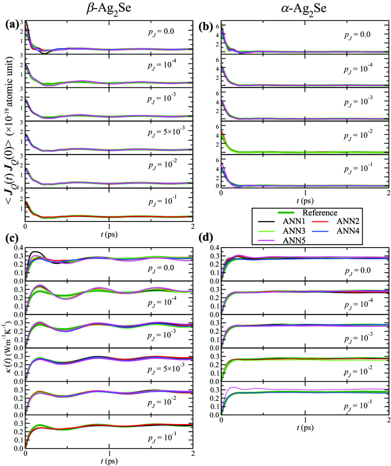
Figure S 3: (a-b) $\langle{\bf{J}}_{Q}(t)\cdot{\bf{J}}_{Q}(0)\rangle$ (atomic unit) and (c-d) $\kappa(t)$ (Wm^-1K^-1) obtained by the EIP of Ag₂Se (Reference, dark green) and trained ANN potentials with heat flux regularization under each $p_{J}$ for $\beta$- and $\alpha$-Ag₂Se. ANN potentials (ANN1-ANN5) are trained with five different initial weight parameters (identified by colors in the figures above).

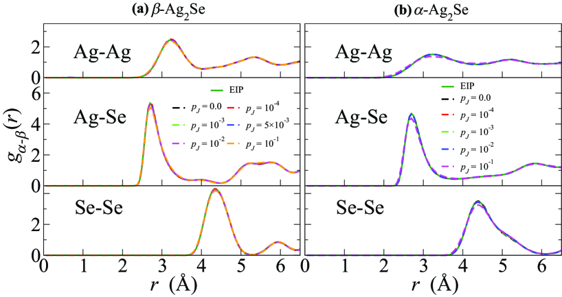
Figure S 4: Partial radial distribution functions $g_{\alpha\mathchar 45\relax\beta}$($r$) for atomic pairings Ag-Ag, Ag-Se, and Se-Se calculated by MD simulations with the EIP of Ag₂Se and ANN potentials with the regularization of each $p_{J}$ for (a) $\beta$- and (b) $\alpha$-Ag₂Se. For each $p_{J}$, the one giving the worst training accuracy for the atomic force was used from the ANN potentials for which the power spectrum could be calculated.

Figure S 5: Mean squared displacements (MSDs) (Ų) of Ag and Se atoms calculated by MD simulations using the EIP of Ag₂Se and ANN potentials with the regularization of each $p_{J}$ for (a) $\beta$- and (b) $\alpha$-Ag₂Se. For each $p_{J}$, the one giving the worst training accuracy for the atomic force was used from the ANN potentials for which the power spectrum could be calculated.

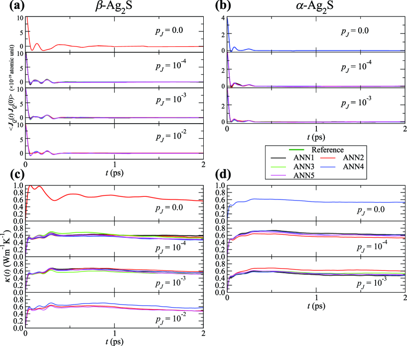
Figure S 6: (a-b) $\langle{\bf{J}}_{Q}(t)\cdot{\bf{J}}_{Q}(0)\rangle$ (atomic unit) and (c-d) $\kappa(t)$ (Wm^-1K^-1) obtained by the trained ANN potentials with heat flux regularization under each $p_{J}$ for $\beta$- and $\alpha$-Ag₂S. ANN potentials (ANN1-ANN5) are trained with five different initial weight parameters (identified by colors in the figures above).

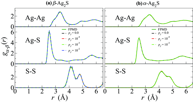
Figure S 7: $g_{\alpha\mathchar 45\relax\beta}$($r$) for atomic pairings Ag-Ag, Ag-S, and S-S calculated in the FPMD simulation and MD simulations with ANN potentials with the regularization of each $p_{J}$ for (a) $\beta$- and (b) $\alpha$-Ag₂S. For each $p_{J}$, the one giving the worst training accuracy for the atomic force was used from the ANN potentials for which the power spectrum could be calculated.

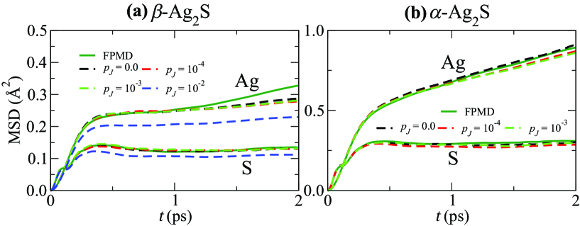
Figure S 8: MSDs (Ų) of Ag and S atoms calculated in the FPMD simulation and MD simulations using the ANN potentials with the regularization of each $p_{J}$ for (a) $\beta$- and (b) $\alpha$-Ag₂S. For each $p_{J}$, the one giving the worst training accuracy for the atomic force was used from the ANN potentials for which the power spectrum could be calculated.

References

References

- Volz and Chen (2000) S. G. Volz and G. Chen, Phys. Rev. B 61, 2651 (2000).
- Kubo (1957) R. Kubo, J. Phys. Soc. Jpn. 12, 570 (1957).
- Green (1952) M. S. Green, J. Chem. Phys. 20, 1281 (1952).
- Morawietz and Artrith (2021) T. Morawietz and N. Artrith, J. Comput. Aided Mol. Des. 35, 557 (2021).
- Tisi et al. (2021) D. Tisi, L. Zhang, R. Bertossa, H. Wang, R. Car, and S. Baroni, Phys. Rev. B 104, 224202 (2021).
- Fan et al. (2021) Z. Fan, Z. Zeng, C. Zhang, Y. Wang, K. Song, H. Dong, Y. Chen, and T. Ala-Nissila, Phys. Rev. B 104, 104309 (2021).
- Verdi et al. (2021) C. Verdi, F. Karsai, P. Liu, R. Jinnouchi, and G. Kresse, Npj Comput. Mater. 7, 156 (2021).
- Li et al. (2020) R. Li, Z. Liu, A. Rohskopf, K. Gordiz, A. Henry, E. Lee, and T. Luo, Appl. Phys. Lett. 117, 152102 (2020).
- Huang et al. (2019) Y. Huang, J. Kang, W. A. Goddard, and L.-W. Wang, Phys. Rev. B 99, 064103 (2019).
- Bosoni et al. (2019) E. Bosoni, D. Campi, D. Donadio, G. C. Sosso, J. Behler, and M. Bernasconi, J. Phys. D: Appl. Phys. 53, 054001 (2019).
- Kim and Kang (2021) S. Kim and J. Kang, Phys. Rev. B 103, 174209 (2021).
- Ercole et al. (2016) L. Ercole, A. Marcolongo, P. Umari, and S. Baroni, J. Low Temp. Phys. 185, 79 (2016).
- Fujii et al. (2020) S. Fujii, T. Yokoi, C. Fisher, H. Moriwake, and M. Yoshiya, Nat. Commun. 11, 1854 (2020).
- Ouyang et al. (2014) T. Ouyang, X. Zhang, and M. Hu, Nanotechnology 26, 025702 (2014).
- Fujii et al. (2018) S. Fujii, M. Yoshiya, and C. Fisher, Scientific Reports 8, 11152 (2018).
- Zhou et al. (2015) Y. Zhou, X. Zhang, and M. Hu, Phys. Rev. B 92, 195204 (2015).
- Zhou and Hu (2015) Y. Zhou and M. Hu, Phys. Rev. B 92, 195205 (2015).
- Sääskilahti et al. (2014) K. Sääskilahti, J. Oksanen, J. Tulkki, and S. Volz, Phys. Rev. B 90, 134312 (2014).
- Irie et al. (2021) A. Irie, S. Fukushima, A. Koura, K. Shimamura, and F. Shimojo, J. Phys. Soc. Jpn 90, 094603 (2021).
- Marques et al. (2019) M. R. G. Marques, J. Wolff, C. Steigemann, and M. A. L. Marques, Phys. Chem. Chem. Phys. 21, 6506 (2019).
- Zhang et al. (2018) L. Zhang, J. Han, H. Wang, R. Car, and W. E, Phys. Rev. Lett. 120, 143001 (2018).
- Novikov et al. (2021) I. S. Novikov, K. Gubaev, E. V. Podryabinkin, and A. V. Shapeev, Mach. Learn.: Sci. Technol. 2, 025002 (2021).
- Rino et al. (1988) J. P. Rino, Y. M. M. Hornos, G. A. Antonio, I. Ebbsjö, R. K. Kalia, and P. Vashishta, J. Chem. Phys. 89, 7542 (1988).
- Shimojo and Okazaki (1991) F. Shimojo and H. Okazaki, J. Phys. Soc. Jpn. 60, 3745 (1991).
- Mahdizadeh and Goharshadi (2014) S. Mahdizadeh and E. Goharshadi, J. Nanoparticle Res. 16, 2553 (2014).
- Zhang and Jiang (2013) X. Zhang and J. Jiang, J. Phys. Chem. C 117, 18441 (2013).
- Hirata et al. (2020) K. Hirata, T. Matsunaga, S. Saurabh, M. Matsunami, and T. Takeuchi, Mater. Trans. 61, 2402 (2020).
- Matsunaga et al. (2021) T. Matsunaga, K. Hirata, S. Singh, M. Matsunami, and T. Takeuchi, Mater. Trans. 62, 16 (2021).
- Artrith and Urban (2016) N. Artrith and A. Urban, Comput. Mater. Sci. 114, 135 (2016).
- Takeshita et al. (2022) Y. Takeshita, K. Shimamura, S. Fukushima, A. Koura, and F. Shimojo, J. Phys. Chem. Solids 163, 110580 (2022).
- Shimamura et al. (2021) K. Shimamura, Y. Takeshita, S. Fukushima, A. Koura, and F. Shimojo, Chem. Phys. Lett. 778, 138748 (2021).
- Shimamura et al. (2020) K. Shimamura, Y. Takeshita, S. Fukushima, A. Koura, and F. Shimojo, J. Chem. Phys. 153, 234301 (2020).
- Behler and Parrinello (2007) J. Behler and M. Parrinello, Phys. Rev. Lett. 98, 146401 (2007).
- Artrith et al. (2017) N. Artrith, A. Urban, and G. Ceder, Phys. Rev. B 96, 014112 (2017).
- Perronace et al. (2002) A. Perronace, G. Ciccotti, F. Leroy, A. H. Fuchs, and B. Rousseau, Phys. Rev. E 66, 031201 (2002).
- Shimojo et al. (2019) F. Shimojo, S. Fukushima, H. Kumazoe, M. Misawa, S. Ohmura, P. Rajak, K. Shimamura, L. Bassman, S. Tiwari, R. K. Kalia, A. Nakano, and P. Vashishta, SoftwareX 10, 100307 (2019).
- Nosé (1984) S. Nosé, Mol. Phys. 52, 255 (1984).
- Okazaki (1967) H. Okazaki, J. Phys. Soc. Jpn. 23, 355 (1967).
- Blöchl (1994) P. E. Blöchl, Phys. Rev. B 50, 17953 (1994).
- Kresse and Joubert (1999) G. Kresse and D. Joubert, Phys. Rev. B 59, 1758 (1999).
- Hohenberg and Kohn (1964) P. Hohenberg and W. Kohn, Phys. Rev. 136, B864 (1964).
- Kohn and Sham (1965) W. Kohn and L. J. Sham, Phys. Rev. 140, A1133 (1965).
- Perdew et al. (1996) J. P. Perdew, K. Burke, and M. Ernzerhof, Phys. Rev. Lett. 77, 3865 (1996).
- Anisimov et al. (1997) V. I. Anisimov, F. Aryasetiawan, and A. I. Lichtenstein, J. Phys. Condens. Matter 9, 767 (1997).
- Fukushima et al. (2019) S. Fukushima, M. Misawa, A. Koura, and F. Shimojo, J. Phys. Soc. Jpn. 88, 115002 (2019).
- Santamaría-Pérez et al. (2012) D. Santamaría-Pérez, M. Marqués, R. Chuliá-Jordán, J. Menendez, O. Gomis, J. Ruiz-Fuertes, J. Sans, D. Errandonea, and J. Recio, Inorg. Chem. 51, 5289 (2012).
- Grimme (2006) S. Grimme, J. Comput. Chem. 27, 1787 (2006).
- Shimojo et al. (2001) F. Shimojo, R. K. Kalia, A. Nakano, and P. Vashishta, Comput. Phys. Commun. 140, 303 (2001).
- Sadanaga and Sueno (1967) R. Sadanaga and S. Sueno, Mineralogical J., 5, 124 (1967).
- Sadovnikov et al. (2018) S. I. Sadovnikov, A. I. Gusev, A. V. Chukin, and A. A. Rempel, Phys. Chem. Chem. Phys. 20, 3847 (2018).
- Fan et al. (2015) Z. Fan, L. F. C. Pereira, H.-Q. Wang, J.-C. Zheng, D. Donadio, and A. Harju, Phys. Rev. B 92, 094301 (2015).
- Marcolongo et al. (2020) A. Marcolongo, L. Ercole, and S. Baroni, J. Chem. Theory Comput. 16, 3352 (2020).
- Shimamura et al. (2019) K. Shimamura, S. Fukushima, A. Koura, F. Shimojo, M. Misawa, R. K. Kalia, A. Nakano, P. Vashishta, T. Matsubara, and S. Tanaka, J. Chem. Phys. 151, 124303 (2019).
- Zhou et al. (2020) W.-X. Zhou, D. Wu, G. Xie, K.-Q. Chen, and G. Zhang, ACS Omega 5, 5796 (2020).

References

- Rino et al. (1988) J. P. Rino, Y. M. M. Hornos, G. A. Antonio, I. Ebbsjö, R. K. Kalia, and P. Vashishta, J. Chem. Phys. 89, 7542 (1988).
- Takeshita et al. (2022) Y. Takeshita, K. Shimamura, S. Fukushima, A. Koura, and F. Shimojo, J. Phys. Chem. Solids 163, 110580 (2022).
- Shimamura et al. (2021) K. Shimamura, Y. Takeshita, S. Fukushima, A. Koura, and F. Shimojo, Chem. Phys. Lett. 778, 138748 (2021).
- Lee et al. (2020) D. Lee, K. Lee, D. Yoo, W. Jeong, and S. Han, Comput. Mater. Sci. 181, 109725 (2020).
- Shimamura et al. (2019) K. Shimamura, S. Fukushima, A. Koura, F. Shimojo, M. Misawa, R. K. Kalia, A. Nakano, P. Vashishta, T. Matsubara, and S. Tanaka, J. Chem. Phys. 151, 124303 (2019).
- Zhang et al. (2018) L. Zhang, J. Han, H. Wang, R. Car, and W. E, Phys. Rev. Lett. 120, 143001 (2018).