Evidence of photosphere emission origin for gamma-ray burst prompt emission

Abstract

The physical origins of gamma-ray burst (GRB) prompt emission (photosphere or synchrotron) are still subject to debate, after more than five decades. Here, we find that many of the observed characteristics of 15 long GRBs, which have the highest prompt emission efficiency $\epsilon_{\gamma}$ ($\epsilon_{\gamma}\gtrsim 80\%$), strongly support photosphere (thermal) emission origin, in the following ways: (1) the relation between $E_{\text{p}}$ and $E_{\text{iso}}$ is almost $E_{\text{p}}\propto(E_{\text{iso}})^{1/4}$ and the dispersion is quite small; (2) the simple power-law shape of the X-ray afterglow light curves and the presence of significant reverse shock signals in the optical afterglow light curves; (3) the best fits using the cutoff power-law model for the time-integrated spectra; and (4) the consistent efficiency from observations (with $E_{\text{iso}}/E_{k}$) and the predictions from the photosphere emission model (with $\eta/\Gamma$). We then further investigate the characteristics of the long GRBs for two distinguished samples ($\epsilon_{\gamma}\gtrsim 50\%$ and $\epsilon_{\gamma}\lesssim 50\%$). It is found that the different distributions for $E_{\text{p}}$ and $E_{\text{iso}}$, and the similar observed efficiency (from the X-ray afterglow) and theoretically predicted efficiency (from the prompt emission or the optical afterglow), follow the predictions of the photosphere emission model well. Also, based on the same efficiency, we derive an excellent correlation of $\Gamma\propto E_{\text{iso}}^{1/8}E_{\text{p}}^{1/2}/(T_{90})^{1/4}$ to estimate $\Gamma$. Finally, we show that different distributions for $E_{\text{p}}$ and $E_{\text{iso}}$, and the consistent efficiency, exist for short GRBs. We also give a natural explanation of the extended emission ($\epsilon_{\gamma}\lesssim 50\%$) and the main pulse ($\epsilon_{\gamma}\gtrsim 50\%$).

1. INTRODUCTION

More than 50 yr after its discovery, the radiation mechanism of gamma-ray burst (GRB) prompt emission (photosphere emission or synchrotron emission) still remains unidentified (e.g., Mészáros, 2002; Zhang & Yan, 2011; Uhm & Zhang, 2014; Geng et al., 2018, 2019; Lin et al., 2018; Zhang et al., 2018a, b, 2021; Li et al., 2019b, 2021; Burgess et al., 2020; Yang et al., 2020; Zhang, 2020; Iyyani & Sharma, 2021; Vyas et al., 2021; Zhang et al., 2021b; Vereshchagin et al., 2022). The photospheric emission is the basic prediction of the classical fireball model (Goodman, 1986; Paczynski, 1986) for a GRB, because the optical depth $\tau$ at the jet base is much larger than unity (e.g. Piran, 1999). As the fireball expands, the optical depth drops down. The internally trapped thermal photons finally escape at the photosphere ($\tau=1$). Indeed, based on the spectral analysis, a quasi-thermal component has been found in several Swift GRBs (Ryde, 2004, 2005; Ryde & Pe’er, 2009) and Fermi GRBs (Guiriec et al., 2011, 2013; Axelsson et al., 2012; Ghirlanda et al., 2013; Larsson et al., 2015; Tang et al., 2021; Deng et al., 2022; Wang et al., 2022; Zhao et al., 2022), especially in GRB 090902B (Abdo et al., 2009; Ryde et al., 2010; Zhang, 2011). But whether the typically observed Band function (a smoothly joint broken power law; Band et al. 1993) or a cutoff power law (CPL) can be explained by the photosphere emission, namely the photospheric emission model, remains unknown (e.g., Abramowicz et al., 1991; Thompson, 1994; Mészáros & Rees, 2000; Rees & Mészáros, 2005; Pe’er & Ryde, 2011; Fan et al., 2012; Lazzati et al., 2013; Ruffini et al., 2013; Bégué & Pe’er, 2015; Gao et al., 2015; Pe’er et al., 2015; Ryde et al., 2017; Acuner & Ryde, 2018; Hou et al., 2018; Meng et al., 2018, 2019, 2022; Li, 2019a, c, 2020; Acuner et al., 2020; Dereli-Bégué et al., 2020; Vereshchagin & Siutsou, 2020; Wang et al., 2020; Parsotan & Lazzati, 2022; Song & Meng, 2022). If this scenario is true, the quasi-thermal spectrum should be broadened. Theoretically, two different broadening mechanisms have been proposed (see Appendix A): subphotospheric dissipation (namely, the dissipative photosphere model; Rees & Mészáros 2005; Giannios & Spruit 2007; Vurm & Beloborodov 2016; Beloborodov 2017; Bhattacharya et al. 2018; Bhattacharya & Kumar 2020) or geometric broadening (namely, the probability photosphere model; Pe’er 2008; Pe’er & Ryde 2011; Lundman et al. 2013; Deng & Zhang 2014; Meng et al. 2018, 2019, 2022).

Previously, some of the implications of the statistical properties of the spectral analysis results for a large GRB sample have appeared to support the photosphere emission model. First, lots of bursts have a low-energy spectral index $\alpha$ that is harder than the death line (or the maximum value, $\alpha$= $-$2/3) of the basic synchrotron model, especially for short GRBs and the peak-flux spectrum (Kaneko et al., 2006; Zhang et al., 2011; Burgess et al., 2017). Second, the spectral width is found to be quite narrow for a significant fraction of GRBs (Axelsson & Borgonovo, 2015; Yu et al., 2015). Third, for half or more of GRBs, the CPL is the best-fit empirical model (Goldstein et al., 2012; Gruber et al., 2014; Yu et al., 2016), indicating that the photosphere emission model can naturally interpret their high-energy spectra. Here, we find more convincing evidence for the photosphere emission origin (especially the probability photosphere model) of GRB prompt emission, by obtaining the prompt efficiency $\epsilon_{\gamma}$.

The paper is organized as follows. In Section 2, we state the data accumulation and the scaling relations predicted by the photosphere model. In Section 3, we describe the evidence from long GRBs with extremely high prompt efficiency $\epsilon_{\gamma}$ ($\epsilon_{\gamma}\gtrsim 80\%$). Then, in Section 4, the evidence from long GRBs with $\epsilon_{\gamma}\gtrsim 50\%$ and $\epsilon_{\gamma}\lesssim 50\%$ is shown. In Section 5, we illustrate the evidence from short GRBs. A brief summary is provided in Section 6.

2. DATA ACCUMULATION AND THE SCALING RELATIONS EXPECTED BY THE FIREBALL MODEL

2.1. Data Accumulation

Table 1The observed quantities for the bursts with extremely high efficiency   ($\epsilon_{\gamma}\gtrsim 80\%$).

GRB	z	$L_{\text{iso}}$	$E_{\text{iso}}$	$L_{\text{X,11}}$	Efficiency	$E_{p,z}$	$\alpha$	$\beta$	best-fitted
		(1052 erg s-1)	(1052 erg)	(1045 erg s-1)		(keV)			model
990705a	0.8424	1.61 $\pm$ 0.15c	21.8 $\pm$ 0.8	1.14	0.83 (0.99f)	551 $\pm$ 17	-0.72 $\pm$ 0.03	-2.68 $\pm$ 0.15e
000210a	0.8463	9.76 $\pm$ 0.5c	19.3 $\pm$ 0.5	1.67	0.74 (0.97f)	687 ${}_{-37}^{+39}$
060927b	5.47	10.8 $\pm$ 0.8	7.56 $\pm$ 0.46	0.28	0.96	459 $\pm$ 90	-0.81 $\pm$ 0.36
061007b	1.261	10.9 $\pm$ 0.9	101 $\pm$ 1.4	1.11	0.97	965 $\pm$ 27	-0.75 $\pm$ 0.02	-2.79 $\pm$ 0.09
080319Bb	0.9382	10.2 $\pm$ 0.9	142 $\pm$ 3	3.90	0.91	1307 $\pm$ 43	-0.86 $\pm$ 0.01	-3.59 $\pm$ 0.45
080607b	3.0363	225.9 $\pm$ 45.3	186 $\pm$ 10	3.46	0.97	1691 $\pm$ 169	-1.08 $\pm$ 0.06
081203Ab	2.05	2.82 $\pm$ 0.19	35.0 $\pm$ 12.8	1.52	0.90	1541 $\pm$ 756	-1.29 $\pm$ 0.14
110205Ab	2.22	2.51 $\pm$ 0.34	55.9 $\pm$ 5.3	2.12	0.92	715 $\pm$ 238	-1.52 $\pm$ 0.14
110818Ac	3.36	6.76 $\pm$ 0.76	21.7 $\pm$ 1.02	0.99	0.93	799.45 $\pm$ 371.90	-1.19 $\pm$ 0.08		CPLd
120729Aa	0.80		2.3 $\pm$ 1.5	0.034	0.94	559 $\pm$ 57
130606Aa	5.913		28.3 $\pm$ 5.2	1.26	0.95	2032 ${}_{-346}^{+622}$	-1.14 $\pm$ 0.15		CPLe
131108Aa	2.40	26.22 $\pm$ 0.6c	54 $\pm$ 2.4	1.98	0.93	1217 ${}_{-88}^{+105}$	-1.16 $\pm$ 0.07		CPLe
150821Aa	0.755	0.77 $\pm$ 0.03c	15.5 $\pm$ 1.2	1.05	0.78	765 ${}_{-126}^{+188}$	-1.52 $\pm$ 0.05		CPLe
160410Aa,s	1.717		9.3 $\pm$ 1.8	0.44	0.89	3853${}_{-973}^{+1429}$	-0.71 $\pm$ 0.20		CPLe
161014Ac	2.823	5.21 $\pm$ 0.52	9.49 $\pm$ 0.50	0.55	0.90	646.18 $\pm$ 55.13	-0.76 $\pm$ 0.08		CPLd
170214Aa	2.53	30.32 $\pm$ 0.85c	318.43 $\pm$ 0.21	1.94	0.99	1810 $\pm$ 34	-0.98 $\pm$ 0.01	-2.51 $\pm$ 0.10d
130606Aa	5.913		28.3 $\pm$ 5.2	1.26	0.95	2032 ${}_{-346}^{+622}$	-1.14 $\pm$ 0.15		CPLe

^a $E_{\text{iso}}$ and $E_{p,z}$ are taken from Minaev & Pozanenko (2020). ^b $E_{\text{iso}}$, $E_{p,z}$, $L_{\text{iso}}$, $\alpha$ and $\beta$ are taken from Nava et al. (2012). ^c $E_{\text{iso}}$,$E_{p,z}$ and $L_{\text{iso}}$ (or $L_{\text{iso}}$ alone) are taken from Xue et al. (2019). ^d The spectral analysis results are from the Fermi GBM Burst Catalog (von Kienlin et al., 2020). ^e The spectral analysis results are from the Konus/Wind Burst Catalog (Tsvetkova et al., 2017). ^f The extremely high efficiency claimed in Lloyd-Ronning & Zhang (2004). ^s The short GRB.

Generally, the radiation efficiency of the prompt emission $\epsilon_{\gamma}$ is defined as $E_{\gamma}/(E_{\gamma}+E_{k})$. Here, $E_{\gamma}$ is the radiated energy in the prompt phase and $E_{k}$ is the remaining kinetic energy in the afterglow phase.

To obtain $\epsilon_{\gamma}$, the isotropic energy $E_{\text{iso}}$ (namely $E_{\gamma}$) and the $L_{\text{X,11h}}$ (the late-time X-ray afterglow luminosity at 11 hr) data should be accumulated for the GRB sample with the redshift $z$. Because that, $L_{\text{X,11h}}$ is roughly proportional to the $E_{\text{k}}$ (see Appendix B.1).

(1) For 46 long bursts before GRB 110213A, we use the $L_{\text{X,11h}}$ data given in D’Avanzo et al. (2012). Also, $E_{\text{iso}}$, the isotropic luminosity $L_{\text{iso}}$, the peak spectral energy in the rest frame $E_{p,z}$ (or $E_{\text{p}}$), the low-energy spectral index $\alpha$, and the high-energy spectral index $\beta$ are taken from Nava et al. (2012).

(2) For 117 long bursts after GRB 110213A (see Tables 1–3, with $\epsilon_{\gamma}\gtrsim 80\%$, $\epsilon_{\gamma}\lesssim 50\%$, and $\epsilon_{\gamma}\gtrsim 50\%$, respectively), we calculate the $L_{\text{X,11h}}$ following the method (see Appendix B.1) in D’Avanzo et al. (2012). $E_{\text{iso}}$, $L_{\text{iso}}$, $E_{p,z}$, $T_{90,i}$ (the intrinsic duration in the rest frame, or $T_{90}$), and $z$ are mainly taken from Minaev & Pozanenko (2020) and Xue et al. (2019).

Our spectral fitting results for the $\epsilon_{\gamma}\gtrsim 80\%$ sample are given in Table 4. And for several bursts of the $\epsilon_{\gamma}\lesssim 50\%$ sample, the perfectly consistent observed efficiency (with $E_{\text{iso}}/E_{k}$) and the theoretically predicted efficiency of the photosphere model (from the prompt emission) are given in Table 5.

In Table 6, for the long-GRB sample with the detection of the peak time of the early optical afterglow (namely $T_{p}$ or $T_{p,op}$, to obtain the Lorentz factor of the outflow $\Gamma$ and then $(R_{\text{ph}}/R_{s})^{-2/3}$) in Ghirlanda et al. (2018), the consistent predicted efficiency (from the prompt emission and the optical afterglow) of the photosphere model is provided. Also, $E_{\text{iso}}$, $L_{\text{iso}}$, and $E_{p,z}$ are taken from Ghirlanda et al. (2018). In Table 7, its subsample (9 bursts) with the maximum $\Gamma$ (for fixed $L_{\text{iso}}$; according to the photosphere model, $\epsilon_{\gamma}=50\%$) is provided.

In Table 8, the short-GRB sample (with $L_{\text{X,11h}}$ derived in this work) is given, along with that possessing extended emission. $E_{\text{iso}}$ and $E_{p,z}$ are taken from Minaev & Pozanenko (2020).

$E_{\text{iso}}$ is generally estimated by $E_{\text{iso}}=4\pi D_{L}^{2}S_{\gamma}/(1+z)$, where $S_{\gamma}$ is the time-integral fluence in the $1-10^{4}$ keV energy range in the rest frame (in units of erg cm^-2) and $D_{L}$ is the luminosity distance. $L_{\text{iso}}$ is estimated as $L_{\text{iso}}=4\pi D_{L}^{2}F_{p}$, where $F_{p}$ is the peak flux (in units of erg cm^-2 s^-1). $T_{90,i}$ is calculated as $T_{90,i}=T_{90,\text{ob}}/(1+z)$, where $T_{90,\text{ob}}$ is determined by the time range between the epochs when the accumulated net photon counts reach the $5\%$ level and the $95\%$ level. And $E_{\text{p}}=(1+z)\cdot E_{\text{p},\text{ob}}$, where $E_{\text{p},\text{ob}}$ is determined by the peak energy in the $\nu F_{\nu}$ spectrum.

Typically, the afterglow peak time $T_{p}$ is estimated from the optical afterglow peak time $T_{p,op}$, since the early X-ray afterglow peak can be produced by “internal” mechanisms (such as the prolonged central engine activity) or bright flares. Also, the bursts with an early multipeaked optical light curve or an optical peak preceded by a decreasing light curve should be excluded (see Ghirlanda et al. 2018).

2.2. Scaling Relations Predicted by the Photosphere Model

For the photosphere emission model, $\epsilon_{\gamma}\gtrsim 50\%$ and $\epsilon_{\gamma}\lesssim 50\%$ should correspond to the unsaturated acceleration case ($\Gamma\lesssim\eta$; $R_{\text{ph}}<R_{s}$; $E_{\text{iso}}/E_{\text{k}}=\eta Mc^{2}/\Gamma Mc^{2}=\eta/\Gamma$ $\gtrsim 1$) and the saturated acceleration case ($\Gamma=\eta$; $R_{\text{ph}}>R_{s}$; $E_{\text{iso}}/E_{\text{k}}=[\eta Mc^{2}(R_{\text{ph}}/R_{s})^{-2/3}]/\Gamma Mc^{2}=(R_{\text{ph}}/R_{s})^{-2/3}$ $\lesssim 1$), respectively.

2.2.1 $E_{\text{iso}}/E_{\text{k}}=\eta/\Gamma$ for the unsaturated acceleration case, corresponding to $\epsilon_{\gamma}\gtrsim 50\%$

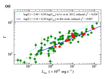
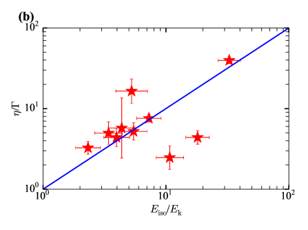
Figure 1.— The $L_{\text{iso}}-\Gamma$ correlation and the $E_{\text{iso}}/E_{\text{k}}$ $-$ $\eta/\Gamma$ correlation for the selected extremely high-efficiency GRBs. (a) The correlation of $L_{\text{iso}}$ and $\Gamma$. Obviously, the tight correlation of $\Gamma\propto(L_{\text{iso}})^{0.29}$ (the red stars, reduced $\chi^{2}=0.007$) is found, which is well consistent with the prediction of the neutrino annihilation from the hyperaccretion disk, $\Gamma\propto(L_{\text{iso}})^{7/27}=(L_{\text{iso}})^{0.26}$. Thus, the jet is likely to be thermal-dominated. The cyan dashed line shows the $L_{\text{iso}}-\Gamma$ correlation found in Lü et al. (2012) (reduced $\chi^{2}=0.038$, for the large $\Gamma$ sample of green circles (Xue et al., 2019)). (b) The correlation of $E_{\text{iso}}/E_{\text{k}}$ and $\eta/\Gamma$. A significant linear correlation is found, and they are almost the same when we take $E_{\text{k,52}}=5\ast L_{\text{X,45}}$ (reduced $\chi^{2}=0.138$). This is well consistent with the predicted $E_{\text{iso}}/E_{\text{k}}=\eta Mc^{2}/\Gamma Mc^{2}=\eta/\Gamma$ by the photosphere emission model in the unsaturated acceleration regime.

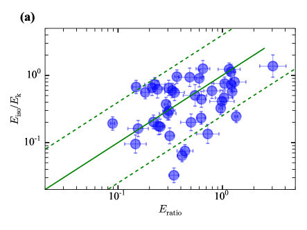
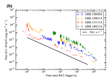
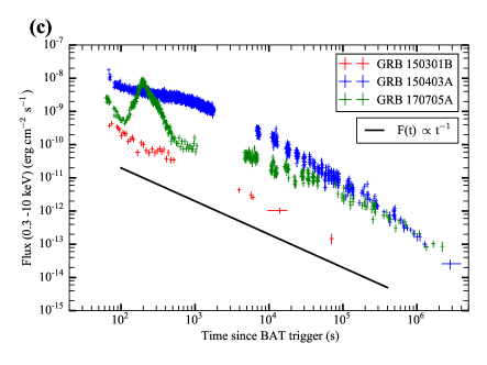
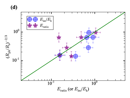
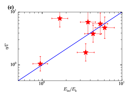
Figure 2.— The similar observed efficiency (with $E_{\text{iso}}/E_{\text{k}}$ from the X-ray afterglow) and theoretically predicted efficiency (from the prompt emission or the optical afterglow) by the photosphere emission model for the bursts after GRB 110213A. (a) The distribution of $E_{\text{ratio}}$ ($E_{\text{ratio}}=[(E_{\text{p}}/2.7k)^{4}\ast(4\pi r_{1}^{2}ac)/E_{\text{iso}}]^{1/3}$, from the prompt emission) and $E_{\text{iso}}/E_{\text{k}}$ for the $\epsilon_{\gamma}\lesssim 50\%$ sample (see Table 2). They are found to be well centered around the equal-value line, and have a linear correlation (reduced $\chi^{2}=0.172$). The dispersion is likely to be caused by the estimation error for $E_{\text{k}}$, since many X-ray afterglow light curves are not the power law with a slope of $-1$. (b) and (c) The X-ray afterglow light curves for the bursts (7 bursts) with almost same $E_{\text{ratio}}$ and $E_{\text{iso}}/E_{\text{k}}$ (see Table 5). We find all these light curves do have the power-law shape with a slope of $\sim$ $-1$. (d) The distribution of $E_{\text{ratio}}$, $E_{\text{iso}}/E_{\text{k}}$ and $(R_{\text{ph}}/R_{s})^{-2/3}$ for the sample (6 bursts, see Table 2) with detections of peak time of the optical afterglow (to estimate the $\Gamma$ and thus $(R_{\text{ph}}/R_{s})^{-2/3}$). It is found that 1 burst has the almost same values for these three quantities and the other 5 bursts have the almost same values for two quantities of them (reduced $\chi^{2}=0.089$ for all 12 markers). (e) The consistent efficiency from observation (with $E_{\text{iso}}/E_{k}$) and the prediction of photosphere emission model (with $\eta/\Gamma$) for the $\epsilon_{\gamma}\gtrsim 50\%$ sample with detections of peak time of the optical afterglow (7 bursts, see Table 3; reduced $\chi^{2}=0.120$).

When the outflow Lorentz factor $\Gamma$ at the photosphere radius $R_{\text{ph}}$ is less than the baryon loading $\eta$ ($\eta=E/Mc^{2}$, where $E$ and $M$ are the injected energy and the baryon mass at the outflow base, respectively), the photosphere emission is in the unsaturated acceleration case (or $R_{\text{ph}}<R_{s}$; where $R_{s}=\eta r_{0}$, and $r_{0}$ is the initial acceleration radius). In this case, $\Gamma=R_{\text{ph}}/r_{0}$.

For the unsaturated acceleration case, the observed temperature $T_{\text{ob}}$ $=$ $D\cdot$ $T_{\text{comoving}}=$ $\Gamma\cdot$ ($T_{0}/\Gamma)=T_{0}$. Here, $D$ is the Doppler factor, $T_{\text{comoving}}$ is the photon temperature in the outflow comoving frame, and $T_{0}$ is the temperature at the outflow base $r_{0}$. Thus, $E_{\text{iso}}=E=\eta Mc^{2}$. Also, because all the thermal energy is released at the photosphere radius (where there is no remaining energy to accelerate the jet), the Lorentz factor in the afterglow phase will remain as $\Gamma$, namely $E_{\text{k}}=\Gamma Mc^{2}$. So we should have $E_{\text{iso}}/E_{\text{k}}=\eta Mc^{2}/\Gamma Mc^{2}=\eta/\Gamma$ $\gtrsim 1$ (see Figure 1(b) and 2(e)), corresponding to $\epsilon_{\gamma}\gtrsim 50\%$.

2.2.2 $E_{\text{p}}\propto(E_{\text{iso}})^{1/4}$ for $\epsilon_{\gamma}\gtrsim 50\%$

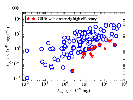
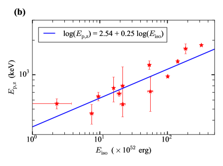
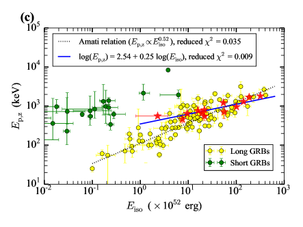
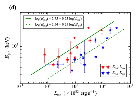
Figure 3.— The $E_{\text{p}}\propto(E_{\text{iso}})^{1/4}$ and $E_{\text{p}}\propto(L_{\text{iso}})^{1/4}$ relations for the GRBs with the highest prompt efficiency $\epsilon_{\gamma}$ ($\epsilon_{\gamma}\gtrsim 80\%$; see Table 1). (a) The $E_{\text{iso}}$ and calculated $L_{\text{X,11h}}$ (the late-time X-ray afterglow luminosity at 11 hours) distribution for the whole GRB sample used (117 bursts, after GRB 110213A) with redshift. The red stars with the smallest $L_{\text{X,11h}}$ represent the bursts with the highest prompt efficiency. (b) The $E_{\text{p}}$ and $E_{\text{iso}}$ distribution for the selected 15 long GRBs. The best-fit result is log ($E_{\text{p}}$) $=2.54+0.25\log$ ($E_{\text{iso}}$), quite consistent with the $E_{\text{p}}\propto(E_{\text{iso}})^{1/4}$ relation predicted by the photosphere (thermal) emission model. (c) Comparison of the $E_{\text{p}}$ and $E_{\text{iso}}$ distributions for the selected GRBs (red stars) and the large sample of long GRBs (see Figure 3 in Zhang et al. (2018b)) (yellow circles). Obviously, the dispersion for the selected GRBs is quite small (reduced $\chi^{2}=0.009$) relative to that for the large sample (reduced $\chi^{2}=0.035$). The black dotted line shows the Amati relation (Amati et al., 2002) for the large sample. (d) Comparison of the $E_{\text{p}}$ $-$ $L_{\text{iso}}$ distribution (red stars) and the $E_{\text{p}}$ $-$ $E_{\text{iso}}$ distribution (blue stars) for the selected GRBs. Likewise, the $E_{\text{p}}\propto(L_{\text{iso}})^{1/4}$ relation exists. The best-fit result is log ($E_{\text{p}}$) $=2.75+0.23\log$ ($L_{\text{iso}}$). And the dispersion (reduced $\chi^{2}=0.012$) is found to be similar to that of $E_{\text{p}}\propto(E_{\text{iso}})^{1/4}$.

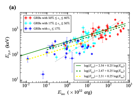
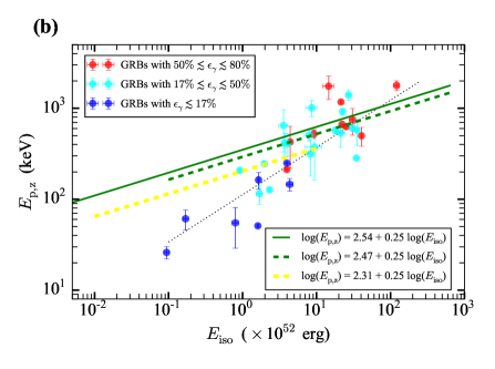
Figure 4.— The different distributions for $E_{\text{p}}$ and $E_{\text{iso}}$ of the two distinguished samples ($\epsilon_{\gamma}\gtrsim 50\%$ and $\epsilon_{\gamma}\lesssim 50\%$; see Tables 2 and 3) for the long GRBs. (a) The $E_{\text{p}}$ and $E_{\text{iso}}$ distribution for the bursts after GRB 110213A (117 bursts, with $L_{\text{X,11h}}$ derived in this work). For the $\epsilon_{\gamma}\gtrsim 50\%$ (red circles) sample, the best-fit result is log ($E_{\text{p}}$) $=2.47+0.25\log$ ($E_{\text{iso}}$) (reduced $\chi^{2}=0.039$; for the black dotted line of the typical Amati relation, reduced $\chi^{2}=0.079$), well consistent with the predicted $E_{\text{p}}\propto(E_{\text{iso}})^{1/4}$ by the photosphere emission model. For the $\epsilon_{\gamma}\lesssim 50\%$ (blue and cyan circles) sample, the up-most distribution is found well around $\log$ ($E_{\text{p}}$) $=2.54+0.25\log$ ($E_{\text{iso}}$), and the best-fit result is log ($E_{\text{p}}$) $=2.31+0.26\log$ ($E_{\text{iso}}$) (reduced $\chi^{2}=0.076$; for the typical Amati relation, reduced $\chi^{2}=0.113$), quite below that. (b) The $E_{\text{p}}$ and $E_{\text{iso}}$ distribution for the bursts before GRB 110213A (46 bursts, with $L_{\text{X,11h}}$ given in D’Avanzo et al. 2012). The different distributions for $E_{\text{p}}$ and $E_{\text{iso}}$ of the two distinguished samples ($\epsilon_{\gamma}\gtrsim 50\%$ and $\epsilon_{\gamma}\lesssim 50\%$) are also found, similar to the distributions for the bursts after GRB 110213A.

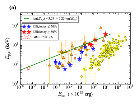
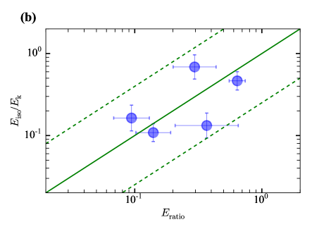
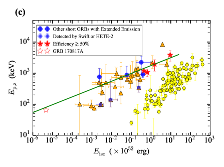
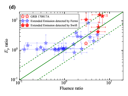
Figure 5.— Evidence from the short GRBs (see Table 8). (a) The different distributions of $E_{\text{p}}$ and $E_{\text{iso}}$ for the two distinguished samples: $\epsilon_{\gamma}\gtrsim 50\%$ (red stars) and $\epsilon_{\gamma}\lesssim 50\%$ (blue stars). (b) The distribution of $E_{\text{ratio}}$ and $E_{\text{iso}}/E_{\text{k}}$ for the $\epsilon_{\gamma}\lesssim 50\%$ sample (reduced $\chi^{2}=0.140$). (c) The $E_{\text{p}}$ and $E_{\text{iso}}$ distribution of the main pulse for other 7 bursts (blue circles and boxes), which have extended emission (see Minaev & Pozanenko 2020) and lack efficiency. Note that all the 5 bursts of the $\epsilon_{\gamma}\gtrsim 50\%$ sample (red stars) have extended emission, including GRB 170817A. (d) The comparison of the ratios of the $E_{\text{p}}$ and the fluence (or $E_{\text{iso}}$) for the main pulse and the extended emission of a large extended emission sample (reduced $\chi^{2}=0.196$), including the bursts without redshift (blue stars).

For the photosphere emission model, the peak energy of the observed spectrum $E_{\text{p}}$ corresponds to the temperature of the observed blackbody $T_{\text{ob}}$. In the unsaturated regime ($R_{\text{ph}}<R_{s}$, $\epsilon_{\gamma}\gtrsim 50\%$), $T_{\text{ob}}=T_{0}$. Since $T_{0}\propto E^{1/4}\propto(E_{\text{iso}})^{1/4}$, we should have $E_{\text{p}}\propto(E_{\text{iso}})^{1/4}$ (see Figures 3–5; for $\epsilon_{\gamma}\gtrsim 80\%$ and $\epsilon_{\gamma}\gtrsim 50\%$ of long GRBs, and short GRBs).

2.2.3 For $\epsilon_{\gamma}\lesssim 50\%$, $E_{\text{iso}}=E\cdot(R_{\text{ph}}/R_{s})^{-2/3}$ and $E_{\text{p}}\propto E^{1/4}\cdot(R_{\text{ph}}/R_{s})^{-2/3}$

For $\epsilon_{\gamma}\lesssim 50\%$ ($R_{\text{ph}}>R_{s}$), the outflow performs adiabatic expansion at $r>R_{s}$. Thus, the comoving temperature decreased as $T_{\text{comoving}}=(T_{0}/\Gamma)\cdot(r/R_{s})^{-2/3}$. The escaped photons at $R_{\text{ph}}$ have $E_{\text{iso}}=E\cdot(R_{\text{ph}}/R_{s})^{-2/3}$ and $E_{\text{p}}=2.7kT_{0}\cdot(R_{\text{ph}}/R_{s})^{-2/3}\propto E^{1/4}\cdot(R_{\text{ph}}/R_{s})^{-2/3}$. So, $E_{\text{iso}}$ and $E_{\text{p}}$ should both decrease by the same factor of $(R_{\text{ph}}/R_{s})^{-2/3}$, compared with the $E_{\text{p}}\propto(E_{\text{iso}})^{1/4}$ correlation for $\epsilon_{\gamma}\gtrsim 50\%$ (see Figures 4 and 5).

2.2.4 For $\epsilon_{\gamma}\lesssim 50\%$, $E_{\text{iso}}/E_{\text{k}}=(R_{\text{ph}}/R_{s})^{-2/3}=[(E_{\text{p}}/2.7k)^{4}\ast(4\pi r_{1}^{2}ac)/E_{\text{iso}}]^{1/3}$

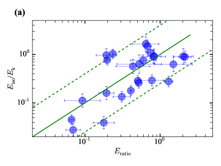
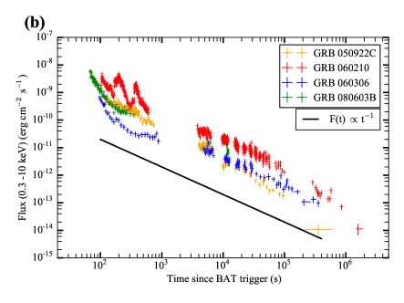
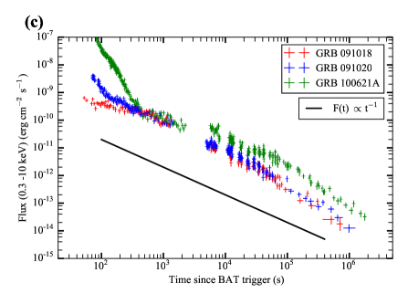
Figure 6.— The similar observed efficiency (with $E_{\text{iso}}/E_{\text{k}}$ from the X-ray afterglow) and theoretically predicted efficiency (from the prompt emission) for the bursts before GRB 110213A (with $L_{\text{X,11h}}$ given in D’Avanzo et al. 2012). (a) The distribution of $E_{\text{ratio}}$ and $E_{\text{iso}}/E_{\text{k}}$ for the $\epsilon_{\gamma}\lesssim 50\%$ sample, which is found to be well centered around the equal-value line and have a linear correlation (reduced $\chi^{2}=0.160$). (b), (c) The X-ray afterglow light curves for the bursts (7 bursts) with almost same $E_{\text{ratio}}$ and $E_{\text{iso}}/E_{\text{k}}$ (see Table 5). We find that all these light curves do have a power-law shape with a slope of $\sim$ $-1$.

For the $\epsilon_{\gamma}\lesssim 50\%$ sample (saturated acceleration, $E_{\text{k}}=E$), we should have

$$E_{\text{iso}}=E\cdot(R_{\text{ph}}/R_{s})^{-2/3}$$ (1)

and

$$E_{\text{p}} = 2.7kT_{0}\cdot(R_{\text{ph}}/R_{s})^{-2/3}$$ (2)

$$= 2.7k(L/4\pi r_{0}^{2}ac)^{1/4}\cdot(R_{\text{ph}}/R_{s})^{-2/3}$$

$$= 2.7k(E/4\pi r_{1}^{2}ac)^{1/4}\cdot(R_{\text{ph}}/R_{s})^{-2/3}$$

$$= 2.7k(4\pi r_{1}^{2}ac)^{-1/4}\cdot E^{1/4}\cdot(R_{\text{ph}}/R_{s})^{-2/3},$$

here $r_{1}^{2}\simeq r_{0}^{2}\ast T_{90\text{.}}$ From the relation of $\log$ ($E_{\text{p}}$) $=2.54+0.25\log$ ($E_{\text{iso}}$) in Figure 3(b), we obtain $r_{1}=8.45\times 10^{8}$ cm. Then, from Equation (1) and Equation (2), we get

$$(E_{\text{p}})^{4}/E_{\text{iso}}=(2.7k)^{4}\ast(4\pi r_{1}^{2}ac)^{-1}\cdot(R_{\text{ph}}/R_{s})^{-2}\text{,}$$ (3)

thus

$$\ (R_{\text{ph}}/R_{s})^{-2/3}=[(E_{\text{p}}/2.7k)^{4}\ast(4\pi r_{1}^{2}ac)/E_{\text{iso}}]^{1/3}.$$ (4)

Combined with the abovementioned $E_{\text{iso}}/E_{\text{k}}=(R_{\text{ph}}/R_{s})^{-2/3}$, $E_{\text{ratio}}=E_{\text{iso}}/E_{\text{k}}=(R_{\text{ph}}/R_{s})^{-2/3}$ is predicted ($E_{\text{ratio}}=[(E_{\text{p}}/2.7k)^{4}\ast(4\pi r_{1}^{2}ac)/E_{\text{iso}}]^{1/3}$; see Figures 2, and 5–7).

2.2.5 $\Gamma\propto E_{\text{iso}}^{1/8}E_{\text{p}}^{1/2}/(T_{90})^{1/4}$ correlation

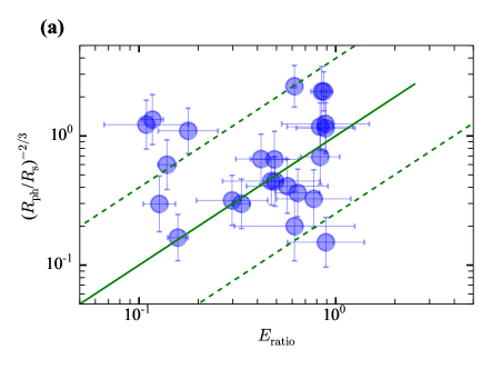
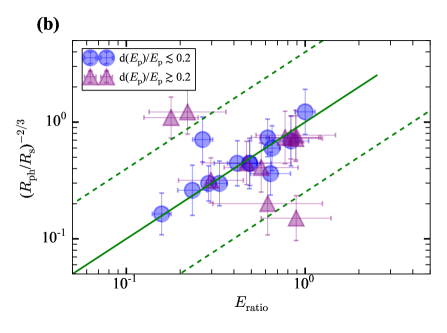
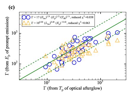
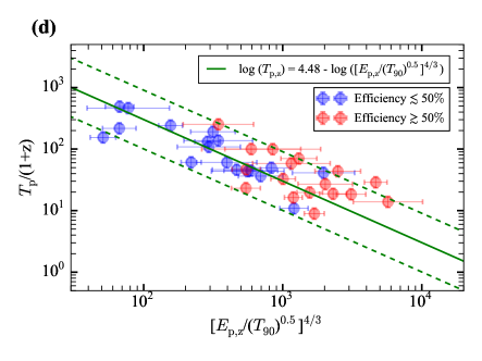
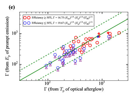
Figure 7.— The tight correlation of $\Gamma\propto E_{\text{iso}}^{1/8}E_{\text{p}}^{1/2}/(T_{90})^{1/4}$ to estimate $\Gamma$, we derived based on the same efficiency of $E_{\text{ratio}}$ and $(R_{\text{ph}}/R_{s})^{-2/3}$ in the $\epsilon_{\gamma}\lesssim 50\%$ case (see Table 6). (a) The distribution of $E_{\text{ratio}}$ and $(R_{\text{ph}}/R_{s})^{-2/3}$ for the selected $\epsilon_{\gamma}\lesssim 50\%$ sample (based on $E_{\text{ratio}}\leq 0.9$; 24 bursts; reduced $\chi^{2}=0.239$). (b) The distributions of $E_{\text{ratio}}$ and $(R_{\text{ph}}/R_{s})^{-2/3}$ for the two sub-samples with smaller $E_{\text{p}}$ errors ($dE_{\text{p}}/E_{\text{p}}\leq 0.2$; blue circles; reduced $\chi^{2}=0.025$) and larger $E_{\text{p}}$ errors ($dE_{\text{p}}/E_{\text{p}}\geq 0.2$; purple triangles; reduced $\chi^{2}=0.228$). (c) A comparison of the $\Gamma$ obtained from the optical afterglow (for 47 bursts in Ghirlanda et al. 2018) and the $\Gamma$ obtained from the prompt emission (orange triangles for $\Gamma=10^{3.33}L_{\text{iso}}^{0.46}E_{\text{p}}^{-0.43}$ and blue circles for $\Gamma=17\cdot E_{\text{iso}}^{1/8}E_{\text{p}}^{1/2}/(T_{90})^{1/4}$). (d) The distribution of $[E_{\text{p}}/(T_{90})^{1/2}]^{4/3}$ and $T_{p}/(1+z)$ for 35 bursts (reduced $\chi^{2}=0.100$). (e) The slightly different constants for the $\epsilon_{\gamma}\lesssim 50\%$ case (Const=19.67, reduced $\chi^{2}=0.034$; Const=16.75, purple triangles, reduced $\chi^{2}=0.048$) and the $\epsilon_{\gamma}\gtrsim 50\%$ case (Const = 16.75).

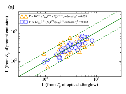
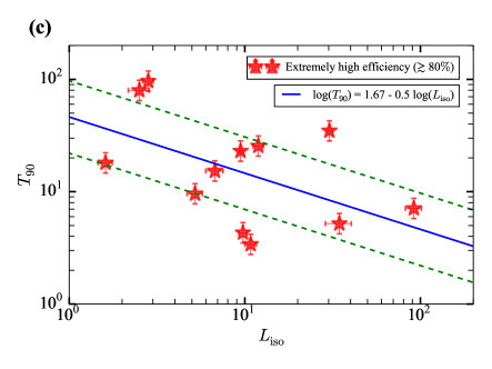
Figure 8.— Comparison of the $\Gamma$ obtained from $\Gamma\propto E_{\text{iso}}^{1/8}E_{\text{p}}^{1/2}/(T_{90})^{1/4}$ and $\Gamma=10^{3.33}L_{\text{iso}}^{0.46}E_{\text{p}}^{-0.43}$ (see Tables 6 and 1). (a) The comparison of the $\Gamma$ obtained from the optical afterglow and the $\Gamma$ obtained from the prompt emission (orange triangles for $\Gamma=10^{3.33}L_{\text{iso}}^{0.46}E_{\text{p}}^{-0.43}$ and blue circles for $\Gamma\propto E_{\text{iso}}^{1/8}E_{\text{p}}^{1/2}/(T_{90})^{1/4}$) for the better sample (35 bursts) in Figure 7(d). The different constants are used for the $\epsilon_{\gamma}\gtrsim 50\%$ and $\epsilon_{\gamma}\lesssim 50\%$ sub-samples. (b) Comparison of the $\Gamma$ obtained from $\Gamma=10^{3.33}L_{\text{iso}}^{0.46}E_{\text{p}}^{-0.43}$ and $\Gamma\propto E_{\text{iso}}^{1/8}E_{\text{p}}^{1/2}/(T_{90})^{1/4}$ for the $\epsilon_{\gamma}\lesssim 50\%$ (cyan triangles; reduced $\chi^{2}=0.043$), the $\epsilon_{\gamma}\gtrsim 50\%$ (orange circles; reduced $\chi^{2}=0.046$) and the high-efficiency ($\epsilon_{\gamma}\gtrsim 80\%$; red stars; reduced $\chi^{2}=0.017$) sub-samples. Obviously, these two estimations are consistent with each other, since they can be transferred with $E_{\text{p}}\propto(E_{\text{iso}})^{1/4}$. (c) The $T_{90}\propto(L_{\text{iso}})^{-0.5}$ correlation (reduced $\chi^{2}=0.174$), found for the high-efficiency sub-sample ($\epsilon_{\gamma}\gtrsim 80\%$).

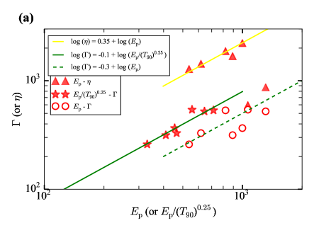
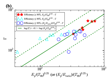
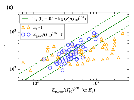
Figure 9.— The tight correlation of $\Gamma\propto$ $E_{\text{p}}/(T_{90})^{1/4}$, predicted by $\Gamma\propto E_{\text{iso}}^{1/8}E_{\text{p}}^{1/2}/(T_{90})^{1/4}$ and $E_{\text{p}}\propto(E_{\text{iso}})^{1/4}$. (a) The distributions of $E_{\text{p}}-\Gamma$ (red circles; reduced $\chi^{2}=0.013$), $E_{\text{p}}-\eta$ (red triangles; reduced $\chi^{2}=0.002$) and $E_{\text{p}}/(T_{90})^{1/4}-\Gamma$ (red stars; reduced $\chi^{2}=0.002$) for the selected $\epsilon_{\gamma}\gtrsim 50\%$ sample with $T_{p}$ detection (7 bursts in Figure 2(e); see Table 3). It is obvious that, the tight correlations of $\Gamma=10^{-0.1}\cdot E_{\text{p}}/(T_{90})^{1/4}$ and $E_{\text{p}}\propto\eta$ (for the 5 bursts with higher efficiency, thus $\eta\propto(E_{\text{iso}})^{1/4}$) are found. (b) The distributions of $(E_{\text{p}}/E_{\text{ratio}})/(T_{90})^{1/4}-\Gamma$ (blue circles; reduced $\chi^{2}=0.031$) and $E_{\text{p}}/(T_{90})^{1/4}-\Gamma$ (cyan triangles) for the selected $\epsilon_{\gamma}\lesssim 50\%$ sample with $T_{p}$ detection (6 bursts in Figure 2(d); see Table 2). The tight correlation of $(E_{\text{p}}/E_{\text{ratio}})/(T_{90})^{1/4}\propto\Gamma$ is found, which is in line with the $E_{\text{p}}/(T_{90})^{1/4}\propto\Gamma$ correlation for the $\epsilon_{\gamma}\gtrsim 50\%$ case. (c) The distribution of $\Gamma-$ $E_{\text{p}}/(T_{90})^{1/4}$ (blue circles; reduced $\chi^{2}=0.025$) for the large sample with $\Gamma$ (47 bursts; see Table 6) in Ghirlanda et al. (2018). For the $\epsilon_{\gamma}\gtrsim 50\%$ case the $E_{\text{p}}$ is re-derived from the $\log$ ($E_{\text{p}}$) $=2.54+0.25\log$ ($E_{\text{iso}}$) correlation (using the $E_{\text{iso}}$), and for the $\epsilon_{\gamma}\lesssim 50\%$ case the $E_{\text{p}}$ is re-derived from $E_{\text{p}}/E_{\text{ratio}}$. Obviously, we find the distribution of $\Gamma$ and $E_{\text{p}}/(T_{90})^{1/4}$ is well centered around $\Gamma=10^{-0.1}\cdot E_{\text{p}}/(T_{90})^{1/4}$ and have a linear correlation.

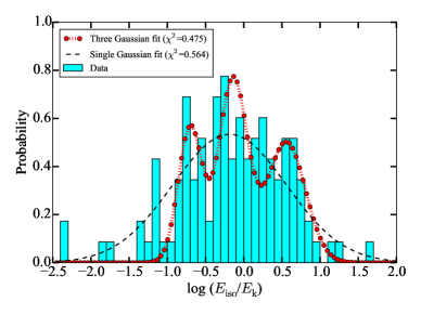
Figure 10.— The distribution of the $E_{\text{iso}}/E_{\text{k}}$ for our whole sample (117 bursts, after GRB 110213A; see Tables 1-3). The mean value is around $\sim$ $10^{-0.2}$ to $10^{-0.3}$, thus indicating the average efficiency of $\epsilon_{\gamma}$ $\sim$ $33\%$ to $40\%$. Also, the distribution seems to consist of three Gaussian distributions (smaller $\chi^{2}$ for $E_{\text{iso}}/E_{\text{k}}\gtrsim 10^{-1.0}$).

As in the previous statement and shown in Figure 7(b), for $\epsilon_{\gamma}\lesssim 50\%$, we have $E_{\text{ratio}}=(R_{\text{ph}}/R_{s})^{-2/3}$. Considering

$$R_{\text{ph}}=\frac{\sigma_{T}}{8\pi m_{p}c^{3}}\frac{L}{\Gamma^{3}},$$ (5)

and $R_{s}$ = $\Gamma\cdot r_{0}$, we have

$$\ [(E_{\text{p}}/2.7k)^{4}\ast(4\pi r_{1}^{2}ac)/E_{\text{iso}}]^{1/3}=(\frac{\sigma_{T}}{8\pi m_{p}c^{3}}\frac{E_{\text{iso}}/T_{90}}{\Gamma^{4}\cdot r_{0}})^{-2/3}.$$ (6)

Thus, we can use the quantities of the prompt emission ($E_{\text{iso}}$, $E_{\text{p}}$ and $T_{90}$) to estimate the Lorentz factor $\Gamma$, just as the obtained $\Gamma=10^{3.33}L_{\text{iso}}^{0.46}E_{\text{p}}^{-0.43}$ from the statistic fitting in Liang et al. (2015) (see Figures 7(c) and 8). Based on Equation (6), we derive

$$\Gamma\propto E_{\text{iso}}^{1/8}E_{\text{p}}^{1/2}/(T_{90})^{1/4}.$$ (7)

Considering the constants, we obtain

$$\Gamma=19.67\cdot E_{\text{iso}}^{1/8}E_{\text{p}}^{1/2}/(T_{90})^{1/4}\text{.}$$ (8)

For the $\epsilon_{\gamma}\gtrsim 50\%$ case, from

$$R_{\text{ph}}=\left[\frac{\sigma_{T}}{6m_{p}c}\frac{L_{\text{iso}}}{4\pi c^{2}\eta}r_{0}^{2}\right]^{1/3}\text{,}$$ (9)

we have

$$\Gamma = R_{\text{ph}}/r_{0}=\left[\frac{\sigma_{T}}{6m_{p}c}\frac{L_{\text{iso}}}{4\pi c^{2}\eta}r_{0}^{2}\right]^{1/3}/r_{0}$$ (10)

$$= \left[\frac{\sigma_{T}}{6m_{p}c}\frac{L_{\text{iso}}}{4\pi c^{2}\eta r_{0}}\right]^{1/3}\text{.}$$

Thus, $L_{\text{iso}}$ $\propto$ $E_{\text{iso}}/(T_{90})$ $\propto$ $\eta\cdot\Gamma^{3}$. Combined with $E_{\text{iso}}/E_{\text{k}}=\eta Mc^{2}/\Gamma Mc^{2}=\eta/\Gamma$, we have $1/T_{90}$ $\propto$ $(1/E_{\text{k}})\cdot\Gamma^{4}$, namely $E_{\text{k}}\propto$ $\Gamma^{4}\cdot T_{90}$. Putting this into $\Gamma\propto(E_{\text{k}})^{1/8}\cdot[T_{p}/(1+z)]^{-3/8}$, we obtain $\Gamma\propto\Gamma^{1/2}\cdot(T_{90})^{1/8}\cdot[T_{p}/(1+z)]^{-3/8}$, namely $\Gamma^{1/2}\cdot(T_{90})^{-1/8}\propto[T_{p}/(1+z)]^{-3/8}$. From Figure 9(a) (discussed in Section 2.2.7), we have $\Gamma\propto$ $E_{\text{p}}/(T_{90})^{1/4}$. So, as in the $\epsilon_{\gamma}\lesssim 50\%$ case, $E_{\text{p}}^{1/2}/(T_{90})^{1/4}\propto[T_{p}/(1+z)]^{-3/8}$ is obtained (as discussed in Section 2.2.6). This means that the Equation (7) is also available for the $\epsilon_{\gamma}\gtrsim 50\%$ case. After considering the constants, we get

$$\Gamma=16.75\cdot E_{\text{iso}}^{1/8}E_{\text{p}}^{1/2}/(T_{90})^{1/4}\text{.}$$ (11)

Note that different constants for the $\epsilon_{\gamma}\lesssim 50\%$ case and the $\epsilon_{\gamma}\gtrsim 50\%$ case are predicted (see Figure 7(d) and (e)). Also, the calculation of $\Gamma$ in Figure 9(a), using the optical afterglow, has assumed an efficiency of $\sim$ $20\%$ (namely, $E_{\text{k}}=5\cdot E_{\text{iso}}$). In fact, when calculating $\Gamma$, we should modify $E_{\text{k}}$ based on the real efficiency ($\eta/\Gamma$). For the $\epsilon_{\gamma}\gtrsim 50\%$ case, we typically have $\eta/\Gamma$ $\sim$ $3.5$ (see Figure 9(a) and Figure 10). Thus, the constant $\sim$ $16.75$ should be $\sim$ $1.4$ times smaller.

2.2.6 $T_{p}/(1+z)\propto[E_{\text{p}}/(T_{90})^{1/2}]^{-4/3}$ correlation

Note that when using the optical afterglow (the peak time $T_{p}$) to obtain $\Gamma$, we have

$$\Gamma \propto (E_{\text{k}})^{1/8}\cdot[T_{p}/(1+z)]^{-3/8}$$ (12)

$$\propto (E_{\text{iso}}/\epsilon_{\gamma})^{1/8}\cdot[T_{p}/(1+z)]^{-3/8}\text{,}$$

where $\epsilon_{\gamma}$ is normally taken as $0.2$. Then, if the Equation (7) is correct, combining Equation (7) and Equation (12) should give (see Figure 7(d))

$$T_{p}/(1+z)\propto[E_{\text{p}}/(T_{90})^{1/2}]^{-4/3}\text{.}$$ (13)

2.2.7 $\Gamma\propto E_{\text{p}}/(T_{90})^{1/4}$ correlation

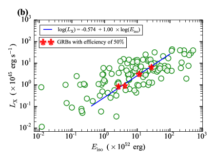
Figure 11.— The $L_{\text{iso}}-\Gamma$ and $E_{\text{iso}}-L_{\text{X,45}}$ distributions for the $\epsilon_{\gamma}=50\%$ sample (see Table 7). (a) The distribution of $L_{\text{iso}}$ and $\Gamma$ for the complete sample (62 bursts) with the detection of $T_{p}$. We select the sample (9 bursts, marked by the red plus) with the maximum $\Gamma$ (for fixed $L_{\text{iso}}$), to check whether their efficiency is $50\%$ as predicted by the photosphere emission model. (b) The distribution of $E_{\text{iso}}$ and $L_{\text{X,45}}$ for the selected sample with the maximum $\Gamma$ (4 bursts with $L_{\text{X,45}}$ detection, red stars). It is found that all these bursts have almost the same efficiency (with $E_{\text{iso}}\propto L_{\text{X}}\propto E_{\text{k}}$, reduced $\chi^{2}=0.008$). Thus, we think that the efficiency $\epsilon_{\gamma}$ for these bursts is likely to be $50\%$ ($E_{\text{iso,52}}=E_{\text{k,52}}\simeq 3.7\ast L_{\text{X,45}}$).

As shown in Figure 4(a), we have $E_{\text{p}}\propto(E_{\text{iso}})^{1/4}$ for both the $\epsilon_{\gamma}\gtrsim 50\%$ case (smaller dispersion) and the $\epsilon_{\gamma}\lesssim 50\%$ case (larger dispersion). Then, with the Equation (7), we should obtain $\Gamma\propto$ $E_{\text{p}}/(T_{90})^{1/4}$. On the other hand, from Figure 1(a) and Figure 11(a) we have approximately $\Gamma\propto(L_{\text{iso}})^{1/4}$, thus $\Gamma\propto$ $E_{\text{p}}/(T_{90})^{1/4}$ is also likely to be obtained (see Figure 9).

2.3. Tightness of the Scaling Relations and Data Errors

To quantitatively measure the tightness of the scaling relations, we calculate the statistical value

$$\chi^{2}=\sum_{i=1}^{N}(\lg y_{i}-a\lg x_{i}-b)^{2},$$ (14)

for each relation of $\lg y=a\lg x-b$ (for example, $\lg E_{\text{p}}=0.25\lg E_{\text{iso}}+2.54$). The reduced $\chi^{2}=\chi^{2}/$degrees of freedom (dof $=N-2$) for each relation is given in the caption for the corresponding figure. Note that $\sqrt{\chi^{2}/\text{dof}}$ is approximate to the typical dispersion measure $\sigma$ (both in units of dex). In Figure 10, for the Gaussian fit, $\chi^{2}=\sum(y_{i}-\bar{y}_{i,\text{model}})^{2}$ is adopted.

To show how well the data follows the predicted relations, the missing errors for the considered quantities are estimated. For the compound quantities (such as $E_{\text{iso}}/E_{\text{k}}$), the errors are estimated by error propagation: $\Delta[\lg(E_{\text{iso}}/E_{\text{k}})]=\Delta[\lg(E_{\text{iso}})-\lg(E_{\text{k}})]=\Delta[\lg(E_{\text{iso}})]+\Delta[\lg(E_{\text{k}})].$ For the $L_{\text{X,11h}}$ derived in this work, $T_{p,op}$, and $T_{90,i}$, the errors at the $90\%$ confidence level ($\sim$ $0.1$ dex) are taken, just as $\Delta(L_{\text{X,11h}})$ given in D’Avanzo et al. (2012).

3. EVIDENCE FROM LONG GRBS WITH EXTREMELY HIGH EFFICIENCY ($\epsilon_{\gamma}\gtrsim 80\%$)

There is much controversy about the spectral differences between the photosphere emission model and the synchrotron emission model, after considering the more natural and complicated physical conditions (jet structure, decaying magnetic field, and so on; Uhm & Zhang 2014; Geng et al. 2018; Meng et al. 2018, 2019, 2022). Nevertheless, a crucial difference between these two models is that the photosphere emission model predicts much higher radiation efficiency $\epsilon_{\gamma}$. The synchrotron emission models mainly include the internal shock model (for a matter-dominated fireball; Rees & Meszaros 1994) and the ICMART model (internal-collision-induced magnetic reconnection and turbulence, for a Poynting flux-dominated outflow; Zhang & Yan 2011). For the internal shock model, since only the relative kinetic energy between different shells can be released, the radiation efficiency is rather low ($\sim 10\%$; Kobayashi et al. 1997). For the ICMART model, the radiation efficiency can be much higher ($\sim 50\%$), and it reaches $\sim 80\%$ in the extreme case. However, the extremely high $\epsilon_{\gamma}$ ($\epsilon_{\gamma}\gtrsim 80\%$) is unlikely to be achieved, because the magnetic reconnection requires some conditions to be triggered, so much magnetic energy is left. For the photosphere emission model, if only the acceleration is in the unsaturated regime ($R_{\text{ph}}<R_{s}$), the radiation efficiency can be close to $100\%$. Thus, in this work, we select the GRBs with extremely high $\epsilon_{\gamma}$ ($\epsilon_{\gamma}\gtrsim 80\%$; see Figure 3(a) and Table 1). Note that the two bursts (GRB 990705 and GRB 000210) that are claimed to have extremely high $\epsilon_{\gamma}$ in Lloyd-Ronning & Zhang (2004) are also included. We then analyze the prompt and afterglow properties of these 15 long GRBs, to confirm the photosphere emission origin.

3.1. Characteristics of Prompt Emission

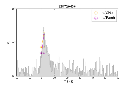
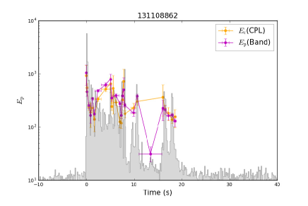
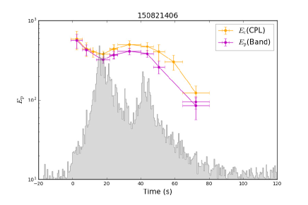
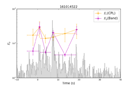
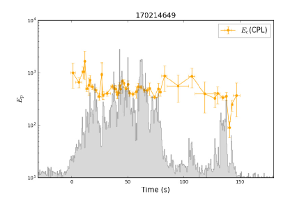
Figure 12.— The $E_{\text{p}}$ evolutions of the time-resolved spectra for 5 extremely high-efficiency GRBs ($\epsilon_{\gamma}\gtrsim 80\%$) detected by Fermi/GBM. The $E_{\text{p}}$ evolutions almost follow the evolution of the flux $F$, consistent with the predicted $E_{\text{p}}\propto F^{1/4}$ by the photosphere (thermal) emission in the unsaturated acceleration regime.

In Figure 3(b), we plot the $E_{\text{p}}$ and $E_{\text{iso}}$ distributions of the selected GRBs (omitting GRB 081203A and GRB 130606A, because of the large $E_{\text{p}}$ error), and we find that they follow the predicted $E_{\text{p}}\propto(E_{\text{iso}})^{1/4}$ relation (see Section 2.2.2) quite well. The best-fit result is log ($E_{\text{p}}$) $=2.54+0.25\log$ ($E_{\text{iso}}$). In Figure 3(c), we compare the $E_{\text{p}}$ and $E_{\text{iso}}$ distributions of the selected GRBs with those of the large sample of long GRBs, and find that the dispersion is quite small relative to that of the large sample.

In Figure 3(d), we plot the $E_{\text{p}}$ and $L_{\text{iso}}$ distributions of the selected GRBs, and find that they also follow the $E_{\text{p}}\propto(L_{\text{iso}})^{1/4}$ relation well. The best-fit result is log ($E_{\text{p}}$) $=2.75+0.23\log$ ($L_{\text{iso}}$). And the dispersion is found to be similar to that of $E_{\text{p}}\propto(E_{\text{iso}})^{1/4}$. Furthermore, based on the best-fit $E_{\text{p}}\sim 10^{2.75}\cdot(L_{\text{iso}})^{1/4}$ and $E_{\text{p}}=2.7kT_{0}=2.7k(L_{\text{iso}}/4\pi r_{0}^{2}ac)^{1/4}$, we obtain the initial acceleration radius $r_{0}\sim 3.21\times 10^{8}$ cm, well consistent with the quite high mean value $\left\langle r_{0}\right\rangle\sim 10^{8.5}$ cm deduced in Pe’er et al. (2015).

In Figure 12, we show the $E_{\text{p}}$ evolutions of the time-resolved spectra for 5 GRBs detected by Fermi/GBM. The $E_{\text{p}}$ evolutions are found to follow the evolution of the flux $F$ quite well (intensity tracking pattern; Liang & Kargatis 1996). This positive correlation is consistent with the abovementioned unsaturated acceleration condition of the photosphere emission. From Tables 1 and 4, we can see that the best-fit spectral model of the time-integrated spectra is the CPL model, or that the high-energy spectral index $\beta$ (using the BAND function to fit) is minimal. Thus, the photosphere emission model can better explain the high-energy spectra of these high-efficiency GRBs.

3.2. Characteristics of Afterglows

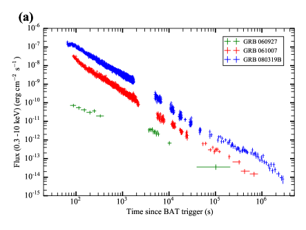
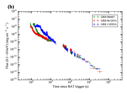
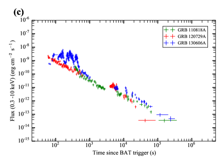
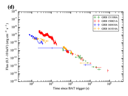
Figure 13.— The X-ray afterglow light curves for the selected extremely high-efficiency GRBs (except for GRB 990705 and GRB 000210). All these light curves appear as a simple power-law shape, without any plateau, steep decay, or significant flare (with weak flare in the early times).

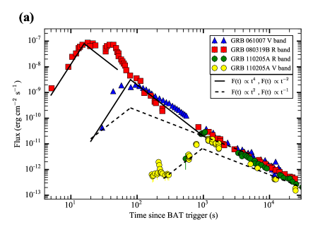
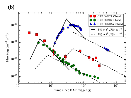
Figure 14.— The optical afterglow light curves for 6 extremely high-efficiency GRBs ($\epsilon_{\gamma}\gtrsim 80\%$) whose early peaks can be detected. All these light curves show significant reverse shock signals. (a) 3 GRBs considered also to have reverse shock signals (with detections of both the rapid rise $f$ $\gtrsim$ $t^{3}$ and fall $f$ $\sim$ $t^{-2}$) in other works (Gao et al. 2015; Yi et al. 2020). (b) 3 GRBs with detection of only the rapid rise $f$ $\gtrsim$ $t^{3}$ or the rapid fall $f$ $\sim$ $t^{-2}$.

Figure 13 shows the X-ray afterglow light curves of the selected GRBs (except for GRB 990705 and GRB 000210). We find that all the X-ray afterglow light curves appear as simple power-law shapes, without any plateau, steep decay (Zhang et al., 2006), or significant flare (with weak flares in the early times). In Figure 14, we show the optical afterglow light curves of 6 GRBs whose early peaks can be detected. All the optical afterglow light curves show significant reverse shock signals. The power-law shape of the X-ray afterglow and the reverse shock in the optical afterglow are the basic predictions (Paczynski & Rhoads, 1993; Mészáros & Rees, 1997; Sari & Piran, 1999) of the classical hot fireball model of GRBs (see Appendices B.2 and B.3). Thus, the jets of these high-efficiency GRBs are likely to be thermal-dominated, and the radiation mechanism of the prompt emission is unlikely to be the ICMART model (for Poynting flux-dominated outflow; Zhang & Yan 2011). Also, considering the high efficiency ($\epsilon_{\gamma}\gtrsim 80\%$), the internal shock model ($\epsilon_{\gamma}$ $\sim 10\%$; Rees & Meszaros 1994; Kobayashi et al. 1997) is unlikely. The prompt emission of these GRBs is likely to be produced by the photosphere emission, then.

In Figure 1(a), we show the correlation of $L_{\text{iso}}$ and $\Gamma$ for the selected GRBs. The $\Gamma$ is obtained by the tight $L_{\text{iso}}-E_{\text{p}}-\Gamma$ correlation (Liang et al. 2015; the values are taken from Xue et al. 2019). In Section 4.3, we find that this estimation is likely to be quite accurate for these high-efficiency GRBs with $E_{\text{p}}\propto(L_{\text{iso}})^{1/4}$. Though 4 GRBs have detections of the peak time of the optical afterglow, we do not use them to estimate the $\Gamma$, because of the significant reverse shock signals. We find that $\Gamma$ is tightly correlated with $L_{\text{iso}}$, $\Gamma\propto(L_{\text{iso}})^{0.29}$. This is well consistent with the prediction of the neutrino annihilation from the hyperaccretion disk (Lü et al., 2012), $\Gamma\propto(L_{\text{iso}})^{7/27}=(L_{\text{iso}})^{0.26}$. This therefore also supports the jets of these GRBs being thermal-dominated.

In Figure 1(b), we show the correlation of $E_{\text{iso}}/E_{\text{k}}$ and $\eta/\Gamma$ (see Section 2.2.1) for the selected GRBs. According to Equation (10), along with $r_{0}\sim 3.21\times 10^{8}$ cm, as derived above, and $L_{\text{iso}}$, we can use $\Gamma$ to obtain the $\eta$ for each burst. We find the obvious linear correlations for $E_{\text{iso}}/E_{\text{k}}$ and $\eta/\Gamma$, and they are almost the same (aside from 3 bursts: note that we obtain 4 bursts that are almost the same when we take $r_{0}=3.21\times 10^{8}$ cm, and then use the offset from the best-fit $E_{\text{p}}\propto(L_{\text{iso}})^{1/4}$ relation to slightly modify $r_{0}$ for the other bursts, to obtain 3 other bursts that are almost the same) when we take $E_{\text{k,52}}=5\ast L_{\text{X,45}}$ ($E_{\text{k,52}}=E_{\text{k}}/10^{52}$, $L_{\text{X,45}}=L_{\text{X}}/10^{45}$; this is quite close to the derivation of $E_{\text{k,52}}=3.7\ast L_{\text{X,45}}$ described in Section 4.1, and the slight difference is likely to result from the slight error of $\Gamma$ estimated by the $L_{\text{iso}}-E_{\text{p}}-\Gamma$ correlation). Again, this result strongly supports the photosphere emission origin in the unsaturated acceleration regime for these high-efficiency GRBs.

3.3. Discussion of the Probability Photosphere Model and the Dissipative Photosphere Model

According to the above statements, the prompt emission of the selected high-efficiency GRBs is likely to be produced by the photosphere emission in the unsaturated acceleration regime. But noteworthily, from Table 1, we can see that the low-energy spectral index $\alpha$ is quite typical (around $-1$), rather than very hard. This strongly supports that the photosphere emission model having the capacity to produce the observed typical soft low-energy spectrum. Theoretically, the probability photosphere model (with geometric broadening) and the dissipative photosphere model (with subphotospheric energy dissipation) can both achieve this. But for the dissipative photosphere model, the $E_{\text{p}}\propto(E_{\text{iso}})^{1/4}$ relation should be violated, since the inverse Compton scattering below the photosphere radius will change the photon energy (namely $T_{\text{ob}}$ $\neq T_{0}$; see Appendix A). Also, the high-energy spectrum for this model should be a power law, rather than the exponential cutoff. So the characteristics of the selected high-efficiency GRBs favor the probability photosphere model.

4. EVIDENCE FROM LONG GRBS WITH $\epsilon_{\gamma}\gtrsim 50\%$ AND $\epsilon_{\gamma}\lesssim 50\%$

4.1.
$\epsilon_{\gamma}=50\%$ and Maximum $\Gamma$

For the $\epsilon_{\gamma}=50\%$ ($R_{\text{ph}}=R_{s}$) case, with a fixed $L_{\text{iso}}$ the observed Lorentz factor $\Gamma$ in the afterglow phase should be the maximum, because of the following reason. To obtain $\epsilon_{\gamma}<50\%$ $(R_{\text{ph}}>R_{s}$, $R_{\text{ph}}\propto L_{\text{iso}}/\Gamma^{3}$ and $R_{s}=\Gamma\cdot r_{0}$), $\Gamma$ ($\Gamma=\eta$) should be smaller. Conversely, for $\epsilon_{\gamma}>50\%$, $\eta$ should be larger. And in this case, from Equation (10), we have $\Gamma$ $\propto(L_{\text{iso}}/\eta)^{1/3}$, thus $\Gamma$ should also be smaller. Note that this maximum $\Gamma$ exists for the hot fireball, while the corresponding $\epsilon_{\gamma}=50\%$ is the prediction of the photosphere emission origin for the prompt emission. The maximum $\Gamma$ is given as (see also Equation 16 in Ghirlanda et al. 2018)

$$\Gamma_{\max}=\left[\frac{L_{\text{iso}}\sigma_{T}}{8\pi m_{p}c^{3}r_{0}}\right]^{1/4}.$$ (15)

In Figure 11(a), we show the distribution of $L_{\text{iso}}$ and $\Gamma$ for the complete sample (62 bursts), with the detection of the peak time of the early optical afterglow (Ghirlanda et al. 2018; obtaining $\Gamma$). Obviously, with the exception of GRB 080319B (with a strong reverse shock signal) and 4 bursts (peak time is obtained from the Fermi/LAT light curve, and the decay slope of $\sim$ $1.5$ implies that it is likely to be produced by the radiative fireball and the $\Gamma$ should be smaller by a factor of $\sim$ $1.6$, see Ghisellini et al. (2010) and Appendix B.4), the distribution of the maximum $\Gamma$ well follows the predicted $L_{\text{iso}}^{1/4}$ correlation, and only has the difference of a constant $\sim$ $10^{0.1}$ ($1.27$) from the prediction of Equation (15) (the dashed line, $r_{0}\sim 3.21\times 10^{8}$ cm is used based on Figure 3). Note that though the equation for calculating $\Gamma$ is confirmed to act as $\Gamma\propto(E_{\text{k}})^{1/8}\cdot[T_{p}/(1+z)]^{-3/8}$, its constant is highly uncertain (see Table 2 in Ghirlanda et al. (2018)). The constant that is given in other works (with different methods) can be 1.7 (or 0.5) times that used in Ghirlanda et al. (2018). So the above difference ($1.27$) obtained by our work is reasonable, and may be more accurate (since it does not strongly depend on the model assumption; if $r_{0}$ is accurate, then it is likely to be accurate).

Then, we select the sample (9 bursts) with the maximum $\Gamma$ (see Table 7) to check their efficiency properties. In Figure 11(b), we show the distribution of $E_{\text{iso}}$ and $L_{\text{X,45}}$ for this sample (4 bursts with $L_{\text{X,45}}$ detection). Note that we exclude GRB 081007 due to the too small $E_{\text{iso}}$ and GRB 080310 due to the plateau in the early optical afterglow. As expected from the photosphere emission model, all these bursts have almost the same efficiency (with $E_{\text{iso}}\propto L_{\text{X}}\propto E_{\text{k}}$). Thus, we think that the efficiency $\epsilon_{\gamma}$ for these bursts is likely to be $50\%$ ($E_{\text{iso,52}}=E_{\text{k,52}}\simeq 3.7\ast L_{\text{X,45}}$). Note that, based on this, the average derived efficiency ($\epsilon_{\gamma}$ $\sim$ $33\%$ to $40\%$; see Figure 10) for the whole sample (117 bursts) is almost consistent with that given in other works (Lloyd-Ronning & Zhang, 2004; Fan & Piran, 2006; Zhang et al., 2007; D’Avanzo et al., 2012; Wygoda et al., 2016).

4.2. $E_{\text{p}}-E_{\text{iso}}$ Distributions and Consistent Efficiency

Based on the derivation of $E_{\text{k,52}}=3.7\ast L_{\text{X,45}}$ described above, and separated by $E_{\text{iso,52}}=E_{\text{k,52}}=3.7\ast L_{\text{X,45}}$ ($\epsilon_{\gamma}=50\%$) for the distribution of $E_{\text{iso,52}}$ and $L_{\text{X,45}}$ in Figure 11, we obtain two distinguished long-GRB samples ($\epsilon_{\gamma}\lesssim 50\%$, see Table 2; and $\epsilon_{\gamma}\gtrsim 50\%$, see Table 3). Note that we exclude the above high-efficiency sample ($\epsilon_{\gamma}\gtrsim 80\%$) and the sample with $\epsilon_{\gamma}=50\%$.

In Figure 4(a), we show that the best-fit result for the $\epsilon_{\gamma}\gtrsim 50\%$ sample is log ($E_{\text{p}}$) $=2.47+0.25\log$ ($E_{\text{iso}}$), which is consistent with the prediction of the photosphere emission model. Also, this result is almost the same as that for the above high-efficiency sample. The offset from the best-fit result is likely to be caused by a distribution of $r_{0}$ (as for the constrained results in Pe’er et al. 2015). For the $\epsilon_{\gamma}\lesssim 50\%$ sample, $E_{\text{iso}}$ and $E_{\text{p}}$ should both decrease by the same factor of $(R_{\text{ph}}/R_{s})^{-2/3}$ (see Section 2.2.3), compared with the distribution of $\log$ ($E_{\text{p}}$) $=2.54+0.25\log$ ($E_{\text{iso}}$) for the above high-efficiency sample. In Figure 4(a), we show that the upmost distribution for the $\epsilon_{\gamma}\lesssim 50\%$ sample is well around $\log$ ($E_{\text{p}}$) $=2.54+0.25\log$ ($E_{\text{iso}}$), and that the best-fit result (much smaller) is log ($E_{\text{p}}$) $=2.31+0.26\log$ ($E_{\text{iso}}$). The decreases of $E_{\text{iso}}$ and $E_{\text{p}}$ are more obvious when we divide the $\epsilon_{\gamma}\lesssim 50\%$ sample into two subsamples ($\epsilon_{\gamma}\lesssim 17\%$ and $\epsilon_{\gamma}\gtrsim 17\%$).

In Figure 2(a), we show the distributions of $E_{\text{ratio}}$ ($E_{\text{ratio}}=[(E_{\text{p}}/2.7k)^{4}\ast(4\pi r_{1}^{2}ac)/E_{\text{iso}}]^{1/3}$) and $E_{\text{iso}}/E_{\text{k}}$ (implicitly, $E_{\text{k,52}}=3.7\ast L_{\text{X,45}}/((1+z)/2)$ is adopted) for the $\epsilon_{\gamma}\lesssim 50\%$ sample. They are well centered around the equal-value line and have a linear correlation. This is well consistent with the prediction from the photosphere emission model (see Section 2.2.4). The dispersion is likely to be caused by the estimation error for $E_{\text{k}}$ (we have excluded the bursts with large $E_{\text{p}}$ errors of $dE_{\text{p}}/E_{\text{p}}\geq 0.2$), since many X-ray afterglow light curves are quite complex (with plateaus, steep decays, or significant flares). The method of using $L_{\text{X,11h}}$ to estimate $E_{\text{k}}$ should only be completely correct for X-ray afterglows with power-law shapes and slopes of $-1$. To check the origin of the dispersion, we select the bursts with almost the same $E_{\text{ratio}}$ and $E_{\text{iso}}/E_{\text{k}}$ (see Table 5). As expected, we find that all these bursts (7 bursts) have a power-law X-ray afterglow light curve with a slope of $\sim$ $-1$ (shown in Figures 2(b) and (c)).

Also, according to Section 2.2.4, for the $\epsilon_{\gamma}\lesssim 50\%$ sample, we should have $E_{\text{ratio}}=E_{\text{iso}}/E_{\text{k}}=(R_{\text{ph}}/R_{s})^{-2/3}$. To check this, we select the bursts with detections of the peak time of the optical afterglow (using them to estimate the $\Gamma$ and thus $(R_{\text{ph}}/R_{s})^{-2/3}$). Note that since $E_{\text{ratio}}$ and $E_{\text{iso}}/E_{\text{k}}$ are the average results for the whole duration, and $(R_{\text{ph}}/R_{s})^{-2/3}$ $\propto$ $L^{-2/3}$, we use $L=$ $E_{\text{iso}}/T_{90}$ (rather than $L_{\text{iso}}$). In Figure 2(d), we show the distributions of $E_{\text{ratio}}$, $E_{\text{iso}}/E_{\text{k}}$ and $(R_{\text{ph}}/R_{s})^{-2/3}$ for the selected sample (6 bursts). Similar to the above, they are well centered around the equal-value line and have a linear correlation. Also, 1 burst has almost the same values for these three quantities, and the other 5 bursts have almost the same values for two quantities. So the predicted $E_{\text{ratio}}=E_{\text{iso}}/E_{\text{k}}=(R_{\text{ph}}/R_{s})^{-2/3}$ from the photosphere emission model can be well reproduced.

For the $\epsilon_{\gamma}\gtrsim 50\%$ sample, similar to Figure 1(b) (for the high-efficiency GRBs), we should have $E_{\text{iso}}/E_{\text{k}}=\eta/\Gamma$. To check this, we also select the bursts with detections of the peak time of the optical afterglow (using them to estimate $\Gamma$ and thus $\eta$). Note that since $\Gamma$ $\propto$ $L^{1/3}$ and the derived $\Gamma$ is likely to correspond to $L_{\text{iso}}$ (the maximum $L$), we use $L=$ $L_{\text{iso}}$ when calculating $\eta$. In Figure 2(e), we show the distribution of $E_{\text{iso}}/E_{\text{k }}$and $\eta/\Gamma$ for the selected sample (7 bursts). As expected, they are well centered around the equal-value line and have a linear correlation.

The analysis results obtained above are for the sample with $L_{\text{X,11h}}$ as derived in this work (for GRBs after GRB 110213A). For another sample with $L_{\text{X,11h}}$ presented in D’Avanzo et al. (2012) (for GRBs before GRB 110213A), we perform a similar analysis and obtain similar results. For the $\epsilon_{\gamma}\gtrsim 50\%$ sub-sample, the $E_{\text{p}}$ and $E_{\text{iso}}$ distribution is also centered around log ($E_{\text{p}}$) $=2.47+0.25\log$ ($E_{\text{iso}}$) (see Figure 4(b)). For the $\epsilon_{\gamma}\lesssim 50\%$ sub-sample, the decreases of $E_{\text{iso}}$ and $E_{\text{p}}$ are also obvious. Also, the distributions of $E_{\text{ratio}}$ and $E_{\text{iso}}/E_{\text{k}}$ are well centered around the equal-value line, and have linear correlations (see Figure 6(a)). For the selected bursts with almost same $E_{\text{ratio}}$ and $E_{\text{iso}}/E_{\text{k}}$ (see Table 5), all (7 bursts) show a power-law X-ray afterglow light curve with a slope of $\sim$ $-1$ (see Figures 6(b) and (c)).

4.3. The Excellent Derived $\Gamma\propto E_{\text{iso}}^{1/8}E_{\text{p}}^{1/2}/(T_{90})^{1/4}$ Correlation

The small burst number in Figure 2(d) is a result of obtaining both the X-ray afterglow light curve and the detection of the peak time of the early optical afterglow. To further check $E_{\text{ratio}}=E_{\text{iso}}/E_{\text{k}}=(R_{\text{ph}}/R_{s})^{-2/3}$ for the $\epsilon_{\gamma}\lesssim 50\%$ case, we then analyze the complete sample with detections of the peak time of the early optical afterglow (obtaining $\Gamma$ and thus $(R_{\text{ph}}/R_{s})^{-2/3}$; Ghirlanda et al. 2018; see Table 6). Note that the used constant is $1.27$ times that given in Ghirlanda et al. (2018) (see Section 4.1). Though lacking of $E_{\text{iso}}/E_{\text{k}}$ for most bursts in the sample, considering the different distributions of $E_{\text{p}}$ and $E_{\text{iso}}$ for $\epsilon_{\gamma}\lesssim 50\%$ and $\epsilon_{\gamma}\gtrsim 50\%$, we can use the judgment of ($E_{\text{ratio}}\lesssim$ $0.9$) to roughly select the $\epsilon_{\gamma}\lesssim 50\%$ sub-sample. Note that we do not use the bursts without the $E_{\text{p}}$ value in Minaev & Pozanenko (2020) and Xue et al. (2019) due to the large $E_{\text{p}}$ errors, and we move 4 bursts to the $\epsilon_{\gamma}\gtrsim 50\%$ sub-sample based on their detections of $E_{\text{iso}}/E_{\text{k}}$. In Figure 7(a), we show the distribution of $E_{\text{ratio}}$ and $(R_{\text{ph}}/R_{s})^{-2/3}$ for the selected $\epsilon_{\gamma}\lesssim 50\%$ sub-sample (24 bursts). This distribution is roughly centered around the equal-value line, and has a linear correlation. After modifying the $\Gamma$ or $E_{\text{p}}$ based on Figure 2(d) (using $E_{\text{ratio}}=E_{\text{iso}}/E_{\text{k}}=(R_{\text{ph}}/R_{s})^{-2/3}$) for the 6 bursts there, in Figure 7(b), we show the distributions of $E_{\text{ratio}}$ and $(R_{\text{ph}}/R_{s})^{-2/3}$ for the two sub-samples with smaller $E_{\text{p}}$ errors ($dE_{\text{p}}/E_{\text{p}}\leq 0.2$) and larger $E_{\text{p}}$ errors ($dE_{\text{p}}/E_{\text{p}}\geq 0.2$). Obviously, for the sub-sample with smaller $E_{\text{p}}$ errors, the values of $E_{\text{ratio}}$ and $(R_{\text{ph}}/R_{s})^{-2/3}$ are almost the same. Note that we decrease the $\Gamma$ of GRB 090926A by a factor of 1.6, since its peak time is obtained from the LAT light curve and the decay slope of $\sim$ $1.5$ implies that it is likely to be produced by the radiative fireball (Ghisellini et al., 2010). And, for the large offset in Figure 7(b) (the upper offset), we check its (GRB 090618) optical afterglow light curve, and find that the reverse shock signal is significant, thus overestimating the $\Gamma$ and $(R_{\text{ph}}/R_{s})^{-2/3}$.

Based on $E_{\text{ratio}}=(R_{\text{ph}}/R_{s})^{-2/3}$, we derive $\Gamma\propto E_{\text{iso}}^{1/8}E_{\text{p}}^{1/2}/(T_{90})^{1/4}$ (see Equation $(\ref{e})$ and Equation (7) in Section 2.2.5). In Figure 7(c), we show a comparison of the $\Gamma$ obtained from the optical afterglow (for 47 bursts in Ghirlanda et al. 2018) and the $\Gamma$ obtained from the prompt emission (orange triangles for $\Gamma=10^{3.33}L_{\text{iso}}^{0.46}E_{\text{p}}^{-0.43}$ and blue circles for $\Gamma=17\cdot E_{\text{iso}}^{1/8}E_{\text{p}}^{1/2}/(T_{90})^{1/4}$). Obviously, using these two correlations, we can give an approximate estimation for $\Gamma$, both. Furthermore, the Equation (7) derived in our work from the photosphere emission model can give a better estimation for $\Gamma$ (with a smaller reduced $\chi^{2}$).

According to Equation (7), two correlations of $T_{p}/(1+z)\propto[E_{\text{p}}/(T_{90})^{1/2}]^{-4/3}$ (see Section 2.2.6) and $\Gamma\propto$ $E_{\text{p}}/(T_{90})^{1/4}$ (see Section 2.2.7) are predicted, which will be tested in the following section.

4.3.1 $T_{p}/(1+z)\propto[E_{\text{p}}/(T_{90})^{1/2}]^{-4/3}$ test

In Figure 7(d) we show the distribution of $E_{\text{p}}/(T_{90})^{1/2}$ and $T_{p}/(1+z)$ for 35 bursts (we delect 7 bursts with $dE_{\text{p}}/E_{\text{p}}\geq 0.2$ and 5 bursts with LAT light curves, and we modify the $E_{\text{p}}$ or $T_{p}$ for 5 bursts based on Figure 2(d)). Just as predicted, this distribution shows a linear correlation with a slope of $\sim-4/3$, and it is consistent with $T_{p}/(1+z)\propto(E_{\text{p}})^{-1.25}$ presented in Table 1 of Ghirlanda et al. (2018). So Equation (7) is likely to be correct.

Besides, from Figure 7(d), we can see that the $T_{p}$ for the sub-sample of $\epsilon_{\gamma}\gtrsim 50\%$ is a bit larger than that for $\epsilon_{\gamma}\lesssim 50\%$, though both satisfy the $T_{p}/(1+z)\propto[E_{\text{p}}/(T_{90})^{1/2}]^{-4/3}$ correlation. This is well consistent with the slightly different predicted constants of Equation (7) for the $\epsilon_{\gamma}\lesssim 50\%$ case (19.67, see Equation (8)) and the $\epsilon_{\gamma}\gtrsim 50\%$ case (16.75, see Equation (11)).

The smaller constant ($16.75$) for the $\epsilon_{\gamma}\gtrsim 50\%$ case is consistent with the larger $T_{p}$ in Figure 7(d). In Figure 7(e), we show the derived $\Gamma$ using the Equation (8) and the Equation (11), and find that the distribution for the $\epsilon_{\gamma}\lesssim 50\%$ case is better (more symmetric) than that in Figure 7(c).

4.3.2 $\Gamma=10^{-0.1}\cdot E_{\text{p}}/(T_{90})^{1/4}$ correlation

In Figure 9(a), we do find the tight correlation of

$$\Gamma=10^{-0.1}\cdot E_{\text{p}}/(T_{90})^{1/4}$$ (16)

for the $\epsilon_{\gamma}\gtrsim 50\%$ case (with $L_{\text{X,11h}}$ detection). Note that the $E_{\text{p}}$ here is re-derived from the $\log$ ($E_{\text{p}}$) $=2.54+0.25\log$ ($E_{\text{iso}}$) correlation (using the $E_{\text{iso}}$), since the observed $E_{\text{p}}$ with an offset from the above line is likely to arise from the different $r_{0}$ (actually $E_{\text{p}}\propto(E_{\text{iso}}/r_{0}^{2})^{1/4}$) or the error of $E_{\text{p}}$. Besides, we modify the $\Gamma$ (using $E_{\text{iso}}/E_{\text{k}}$, mainly for 3 bursts) based on Figure 2(e). In Figure 9(a), we also show the distributions for $E_{\text{p}}-\Gamma$ and $E_{\text{p}}-\eta$, here $\eta$ is obtained by $\eta/\Gamma=E_{\text{iso}}/E_{\text{k}}$. It is obvious that there is a tight correlation of $E_{\text{p}}\propto\eta$ for the sub-sample (5 bursts) with higher efficiency. This means that $\eta\propto(E_{\text{iso}})^{1/4}$, which is well consistent with the prediction of the neutrino annihilation from the hyperaccretion disk (for the hot fireball).

For the $\epsilon_{\gamma}\lesssim 50\%$ case, since $(E_{\text{p}}/E_{\text{ratio}})\propto(E_{\text{iso}}/E_{\text{ratio}})^{1/4}$ and $\Gamma\propto(L_{\text{iso}}/E_{\text{ratio}})^{1/4}$ we should have $\Gamma\propto$ $(E_{\text{p}}/E_{\text{ratio}})/(T_{90})^{1/4}$. From Figure 9(b) we do find this correlation, which is also in line with that for the $\epsilon_{\gamma}\gtrsim 50\%$ case. Note that we modify the $E_{\text{p}}$ or $\Gamma$ based on Figure 2(d). In Figure 9(c) we show the distribution of $\Gamma-$ $E_{\text{p}}/(T_{90})^{1/4}$ for the large $\Gamma$ sample (47 bursts) in Ghirlanda et al. (2018). Note that for the $\epsilon_{\gamma}\gtrsim 50\%$ case, the $E_{\text{p}}$ is re-derived from the $\log$ ($E_{\text{p}}$) $=2.54+0.25\log$ ($E_{\text{iso}}$) correlation (using the $E_{\text{iso}}$), and for the $\epsilon_{\gamma}\lesssim 50\%$ case, the $E_{\text{p}}$ is re-derived from $E_{\text{p}}/E_{\text{ratio}}$. For the $\epsilon_{\gamma}\gtrsim 50\%$ case, when calculating $\Gamma$, we modify the $E_{\text{k}}$ based on the original $\eta/\Gamma$. Obviously, we find that the distribution of $\Gamma$ and $E_{\text{p}}/(T_{90})^{1/4}$ is well centered around $\Gamma=10^{-0.1}\cdot E_{\text{p}}/(T_{90})^{1/4}$ and shows a linear correlation. Note that the $\Gamma-$ $E_{\text{p}}$ correlation is also found in Ghirlanda et al. (2012).

4.3.3 The consistency of our $\Gamma\propto E_{\text{iso}}^{1/8}E_{\text{p}}^{1/2}/(T_{90})^{1/4}$ correlation and the $\Gamma=10^{3.33}L_{\text{iso}}^{0.46}E_{\text{p}}^{-0.43}$ correlation

For the better sample (35 bursts) in Figure 7(d), in Figure 8(a), we replot the comparison of the $\Gamma$ obtained from the optical afterglow and the $\Gamma$ obtained from the prompt emission (orange triangles for $\Gamma=10^{3.33}L_{\text{iso}}^{0.46}E_{\text{p}}^{-0.43}$ and blue circles for $\Gamma\propto E_{\text{iso}}^{1/8}E_{\text{p}}^{1/2}/(T_{90})^{1/4}$). For the $\epsilon_{\gamma}\gtrsim 50\%$ sub-sample (17 bursts) and the $\epsilon_{\gamma}\lesssim 50\%$ sub-sample (18 bursts), we use the different derived constants. Obviously, the Equation (7) derived in our work gives a much better estimation of $\Gamma$ (with a much smaller reduced $\chi^{2}$, compared with Figure 7(c)). Noteworthily, the $\Gamma=10^{3.33}L_{\text{iso}}^{0.46}E_{\text{p}}^{-0.43}$ correlation obtained from the statistical fitting is actually consistent with our $\Gamma\propto E_{\text{iso}}^{1/8}E_{\text{p}}^{1/2}/(T_{90})^{1/4}$ correlation derived from the photosphere emission model. Because, along with $E_{\text{p}}\propto(E_{\text{iso}})^{1/4}$ (or $E_{\text{p}}\propto(L_{\text{iso}})^{1/4}$; see Figures 3 and 4), they can be transferred to each other, as shown in the following:

$$\Gamma \propto E_{\text{iso}}^{1/8}E_{\text{p}}^{1/2}/(T_{90})^{1/4}$$ (17)

$$\propto (E_{\text{iso}}/T_{90})^{1/8}\cdot E_{\text{p}}^{1/2}/(T_{90})^{1/8},\text{ with\ }E_{\text{p}}\propto(L_{\text{iso}})^{1/4}\text{\ }$$

$$\propto (L_{\text{iso}})^{1/8}\cdot(L_{\text{iso}}^{0.23}\cdot E_{\text{p}}^{-0.43})/(T_{90})^{1/8}$$

$$\propto L_{\text{iso}}^{0.36}\cdot E_{\text{p}}^{-0.43}/(T_{90})^{1/8},\text{ with }T_{90}\propto(L_{\text{iso}})^{-0.5}\text{ }$$

$$\propto L_{\text{iso}}^{0.36}\cdot E_{\text{p}}^{-0.43}/(L_{\text{iso}}^{-0.5})^{1/8}$$

$$\propto L_{\text{iso}}^{0.43}\cdot E_{\text{p}}^{-0.43}.$$

Here, the adopted $T_{90}\propto(L_{\text{iso}})^{-0.5}$ correlation is found from Figure 8(c) for the high-efficiency sub-sample ($\epsilon_{\gamma}\gtrsim 80\%$).

In Figure 8(b), we compare the $\Gamma$ obtained from $\Gamma=10^{3.33}L_{\text{iso}}^{0.46}E_{\text{p}}^{-0.43}$ and the $\Gamma$ obtained from $\Gamma\propto E_{\text{iso}}^{1/8}E_{\text{p}}^{1/2}/(T_{90})^{1/4}$ for the $\epsilon_{\gamma}\gtrsim 50\%$ sub-sample (17 bursts), the $\epsilon_{\gamma}\lesssim 50\%$ sub-sample (18 bursts) and the high-efficiency sub-sample ($\epsilon_{\gamma}\gtrsim 80\%$). Obviously, these two estimations are well centered around the equal-value line and have linear correlations. Furthermore, for the high-efficiency sub-sample, which has the tightest $E_{\text{p}}\propto(E_{\text{iso}})^{1/4}$ correlation (with very small dispersion; see Figure 3), these two estimations are almost identical. For the $\epsilon_{\gamma}\gtrsim 50\%$ sub-sample and the $\epsilon_{\gamma}\lesssim 50\%$ sub-sample, which have larger dispersions for the $E_{\text{p}}\propto(E_{\text{iso}})^{1/4}$ correlation, the above two estimations show larger dispersion, also.

4.4. The Distribution of the $E_{\text{iso}}/E_{\text{k}}$ for the Whole Sample

In Figure 10, we show the distribution of the $E_{\text{iso}}/E_{\text{k}}$ (indicating the efficiency $\epsilon_{\gamma}$) for the whole sample (117 bursts). The average value is around $\sim$ $10^{-0.2}$ to $10^{-0.3}$, thus indicating an average efficiency of $\epsilon_{\gamma}$ $\sim$ $33\%$ to $40\%$. From Figure 10, we also find that the distribution seems to consist of three Gaussian distributions. The high-efficiency peak ($\sim$ $10^{0.6}$) is almost consistent with the $\eta\propto 10^{0.35}\cdot E_{\text{p}}$ and $\Gamma\propto 10^{-0.3}\cdot E_{\text{p}}$ correlations (namely, $E_{\text{iso}}/E_{\text{k}}=\eta/\Gamma$ $\sim$ $10^{0.65}$) in Figure 9(a). Theoretically, for the $\epsilon_{\gamma}>50\%$ case, from Equation (10) and $\eta\propto(L_{\text{iso}})^{1/4}$, we should also have $\Gamma\propto$ $(L_{\text{iso}}/\eta)^{1/3}\propto$ $(L_{\text{iso}}/L_{\text{iso}}^{1/4})^{1/3}\propto(L_{\text{iso}})^{1/4}$. So the high-efficiency peak is predicted to exist. For the $\epsilon_{\gamma}<50\%$ case, $E_{\text{iso}}/E_{\text{k}}=(R_{\text{ph}}/R_{s})^{-2/3}\propto(L_{\text{iso}}/\Gamma^{4})^{-2/3}$. Thus, the low-efficiency peak ($\sim$ $10^{-0.7}$) is the natural result of $\Gamma\propto(L_{\text{iso}})^{1/4}$, where $\Gamma=\eta$.

5. EVIDENCE FROM SHORT GRBS WITH $\epsilon_{\gamma}\gtrsim 50\%$ AND $\epsilon_{\gamma}\lesssim 50\%$.

For the short GRBs, similar to the long GRBs, we use the judgment of $E_{\text{iso,52}}=E_{\text{k,52}}=3.7\ast L_{\text{X,45}}$ ($\epsilon_{\gamma}=50\%$) to obtain the $\epsilon_{\gamma}\gtrsim 50\%$ sample (4 bursts) and the $\epsilon_{\gamma}\lesssim 50\%$ sample (8 bursts; see Table 8). In Figure 5(a), we show the $E_{\text{p}}$ and $E_{\text{iso}}$ distributions for these two distinguished samples. Obviously, the $\epsilon_{\gamma}\gtrsim 50\%$ sample and the up-most distribution for the large sample of short GRBs (Zhang et al., 2018b) (without $L_{\text{X,45}}$ detections for most) do follow the $E_{\text{p}}\propto(E_{\text{iso}})^{1/4}$ correlation, well consistent with the prediction of the photosphere emission model. Noteworthily, the distribution for GRB 170817A well fits the above line (log ($E_{\text{p}}$) $=3.24+0.25\log$ ($E_{\text{iso}}$)), too. For the $\epsilon_{\gamma}\lesssim 50\%$ sample, as predicted, the distribution is below this line (since $E_{\text{p}}$ and $E_{\text{iso}}$ are smaller). Similar to Figure 2(a) (to test whether the $E_{\text{p}}$ and $E_{\text{iso}}$ are both smaller by a factor of $E_{\text{iso}}/E_{\text{k}}=(R_{\text{ph}}/R_{s})^{-2/3}$), in Figure 5(b) we show the distribution of $E_{\text{ratio}}$ ($E_{\text{ratio}}=[(E_{\text{p}}/2.7k)^{4}\ast(4\pi r_{1}^{2}ac)/E_{\text{iso}}]^{1/3}$) and $E_{\text{iso}}/E_{\text{k}}$ for this $\epsilon_{\gamma}\lesssim 50\%$ sample. Note that we exclude 3 bursts with $E_{\text{iso}}\leq 10^{50}$ erg and that we have $r_{1}=3.4\times 10^{7}$ cm here. Again as predicted, they are found to be almost centered around the equal-value line, and have a linear correlation.

Interestingly, we find that all the bursts of the $\epsilon_{\gamma}\gtrsim 50\%$ sample (5 bursts, including GRB 170817A) have extended emission, and the $E_{\text{p}}$ and $E_{\text{iso}}$ distribution in Figure 5(a) is for their main pulse. To further test this finding, in Figure 5(c) we show the $E_{\text{p}}$ and $E_{\text{iso}}$ distribution of the main pulse for 7 other bursts that have extended emission (Minaev & Pozanenko, 2020). It is found that, except for 3 bursts only detected by Swift or HETE-2 (lacking the detections in the high-energy band), other 4 bursts do follow the log ($E_{\text{p}}$) $=3.24+0.25\log$ ($E_{\text{iso}}$) correlation of the $\epsilon_{\gamma}\gtrsim 50\%$ sample, supporting the above finding again. The true $E_{\text{p}}$ values for these 3 outliers are likely to be much larger. According to the above, the main pulse for the short GRBs with extended emission is likely to be produced by the photosphere emission in the unsaturated acceleration regime. Then, considering the smaller values of both the $E_{\text{p}}$ and $E_{\text{iso }}$for their extended emission, we think that the extended emission may be produced by the transition from the unsaturated acceleration to the saturated acceleration ($E_{\text{p}}$ and $E_{\text{iso}}$ are both smaller by the same factor of $E_{\text{iso}}/E_{\text{k}}=(R_{\text{ph}}/R_{s})^{-2/3}$). To test this hypothesis, in Figure 5(d), we show the comparison of the ratios of the $E_{\text{p}}$ and the fluence of the main pulse and the extended emission for a large extended emission sample (including the Swift/BAT bursts with redshift; Gompertz et al. 2020; and the Fermi/GBM bursts without redshift; Lan et al. 2020). As predicted, these two ratios are found to be almost centered around the equal-value line and they have linear correlations.

6. Summary

In this work, after obtaining the prompt emission efficiency of a large GRB sample with redshift, we divide that GRB sample into three sub-samples ($\epsilon_{\gamma}\gtrsim 80\%$, $\epsilon_{\gamma}\gtrsim 50\%$, and $\epsilon_{\gamma}\lesssim 50\%$). Then, the well-known Amati relation (Amati et al., 2002) is well explained by the photosphere emission model. Furthermore, for each sub-sample, the X-ray and optical afterglow characteristics are well consistent with the predictions of the photosphere emission model. Ultimately, large amounts of convincing observational evidence for the photosphere emission model are revealed for the first time.

Appendix A: the probability photosphere model and the dissipative photosphere model

A.1. The probability photosphere model

For the traditional photosphere model, the photosphere emission is all emitted at the photospheric radius $R_{\text{ph}}$, where the optical depth for a photon propagating towards the observer is equal to unity ($\tau=1$). But, if only there is an electron at any position, the photon should have a probability to be scattered there. For an expanding fireball, the photons can be last scattered at any place in the fireball with a certain probability. Thus, the traditional spherical shell photosphere is changed to a probability photosphere, namely the probability photosphere model (Pe’er, 2008). Based on careful theoretical derivation, the probability function $P(r,\Omega)$, donating the probability for a photon to be last scattered at the radius $r$ and angular coordinate $\Omega$, can be given as (Pe’er 2008; Beloborodov 2011; Lundman et al. 2013)

$$P(r,\Omega)=(1+\beta)D^{2}\times\frac{R_{\text{ph}}}{r^{2}}\exp\left(-\frac{R_{\text{ph}}}{r}\right),$$ (18)

where $\beta$ is the jet velocity and $D$ $=[\Gamma(1-\beta\cdot\cos\theta)]^{-1}$ is the Doppler factor.

For the probability photosphere model, the observed photosphere spectrum is the overlapping of a series of blackbodies with different temperatures, thus its low-energy spectrum is broadened. After considering the jet with angular structure (e.g., Dai & Gou, 2001; Rossi et al., 2002; Zhang & Mészáros, 2002), the observed typical low-energy photon index $\alpha\sim-1.0$ (Kaneko et al., 2006; Zhang et al., 2011), spectral evolution and $E_{p}$ evolutions (hard-to-soft evolution or $E_{p}$-intensity tracking; Liang & Kargatis 1996; Lu et al. 2010, 2012) can be reproduced (Lundman et al., 2013; Meng et al., 2019, 2022).

A.2. The dissipative photosphere model

The dissipative photosphere model (or the sub-photosphere model) considers that there is an extra energy dissipation process in the area of moderate optical depth ($1<\tau<10$; the sub-photosphere). Different dissipative mechanisms have been proposed, such as shocks (Rees & Mészáros, 2005), magnetic reconnection (Giannios & Spruit, 2007) and proton–neutron nuclear collisions (Vurm & Beloborodov, 2016; Beloborodov, 2017). Then, relativistic electrons (with a higher temperature than that of the photons) are generated that upscatter the thermal photons to obtain the non-thermal (broadened) high-energy spectrum.

Appendix B: some theoretical descriptions for the afterglow

B.1. The remaining kinetic energy in the afterglow phase ($E_{\text{k}}$) and the isotropic X-ray afterglow luminosity at 11 hours ($L_{\text{X,11h}}$).

In the context of the standard afterglow model (Paczynski & Rhoads, 1993; Mészáros & Rees, 1997), since at a late afterglow epoch (11 hours) the X-ray band is above the cooling frequency $\nu_{c}$, the late-time X-ray afterglow luminosity ($L_{\text{X,11h}}$) only sensitively depends on $E_{\text{k}}$ and $\epsilon_{e}$ (the electron equipartition parameter). Furthermore, the fraction of energy in the electrons ($\epsilon_{e}$) is quite centered around $0.1$, based on the large-sample afterglow analysis. Thus, $E_{\text{k}}$ can be well estimated by the $L_{\text{X,11h}}$ as following (Lloyd-Ronning & Zhang, 2004):

$$E_{\text{k}} = 10^{52}\text{ ergs R}\left[\frac{L_{\text{X,10h}}}{10^{46}\text{ ergs s}^{-1}}\right]^{4/(2+p)}(\frac{1+z}{2})^{-1}$$

$$\times\epsilon_{e,-1}^{4(1-p)/(2+p)}\epsilon_{B,-2}^{(2-p)/(2+p)}t_{10h}^{(3p-2)/(2+p)}\nu_{18}^{2(p-2)/(2+p)}$$

$$\simeq 10^{52}\text{ ergs R}\left[\frac{1.1L_{\text{X,11h}}}{10^{46}\text{ ergs s}^{-1}}\right](\frac{1+z}{2})^{-1}$$

$$\times(\epsilon_{e,-1})^{-1},\text{ (}p\simeq 2\text{)}$$

where $R$ = [$t$(10 h)/$t$(prompt)]${}^{(17/16)\epsilon_{e}}$ $\sim$ $2.27$ is the radiative losses during the first 10 hours after the prompt phase. Note that the derived $E_{\text{k}}$ is $9.2$ times larger in Fan & Piran (2006), since the $\nu_{m}$ (the characteristic frequency corresponding to the minimum electron Lorentz factor) is about one and a half orders smaller. Previously, it had been hard to judge which constant was better. Here, using the method ($\epsilon_{\gamma}=50\%$ and the maximum $\Gamma$; see Section 4.1) in this work, our result ($E_{\text{k,52}}\simeq 3.7\ast L_{\text{X,45}}$) is quite consistent with $E_{\text{k,52}}\simeq 2.5\ast L_{\text{X,45}}$ (Fan & Piran 2006, without the inverse Compton effect).

The isotropic X-ray afterglow luminosity (in the 2-10 keV rest-frame common energy band) at 11 hours (rest frame), $L_{\text{X,11h}}$, is computed from the observed integral 0.3-10 keV unabsorbed fluxes at 11 hours ($F_{\text{X,11h}}$; estimated from the Swift/XRT light curves) and the measured spectral index $\Gamma_{1}$ (from the XRT spectra), along with the luminosity distance $D_{L}$. The equation is as follows (D’Avanzo et al. 2012):

$$L_{\text{X,11h}}(2-10\text{ keV}) = 4\pi D_{L}^{2}\cdot F_{\text{X,11h}}(0.3-10\text{ keV})\cdot$$ (20)

$$\frac{(\frac{10}{1+z})^{2-\Gamma_{1}}\text{ }-(\frac{2}{1+z})^{2-\Gamma_{1}}}{10^{2-\Gamma_{1}}\text{ }-\text{ }0.3^{2-\Gamma_{1}}}.$$

Here, $F_{\text{X,11h}}$ is obtained by interpolating (or extrapolating) the best-fit power law, for the XRT light curve within a selected time range including (or close to) 11 hours, to the 11 hours.

B.2. The power-law shape of the X-ray afterglow predicted by the classical hot fireball.

The “generic” afterglow model (relativistic blastwave theory) for GRB predicts a power-law decaying multi-wavelength afterglow (Paczynski & Rhoads, 1993; Mészáros & Rees, 1997), due to the self-similar nature of the blastwave solution. The observed specific flux is

$$f_{\nu} \propto E_{\text{k}}^{(p+2)/4}\epsilon_{e}^{p-1}\epsilon_{B}^{(p-2)/4}t_{\text{obs}}^{-(3p-2)/4}\nu^{-p/2}$$ (21)

$$\simeq \frac{(\epsilon_{e}E_{\text{k}})}{t_{\text{obs}}}\nu^{-1},(p\simeq 2).$$

This power-law behavior ($f$ $\sim$ $t_{\text{obs}}^{-1}$) is well consistent with the observations of the optical and radio afterglows. But several surprising emission components (the steep decay $f$ $\sim$ $t_{\text{obs}}^{-3}$ phase, the plateau $f$ $\sim$ $t_{\text{obs}}^{-0.5}$ phase, and the flare) in the early X-ray afterglow are revealed by the Swift observations (Zhang et al., 2006), which are not predicted by the above standard (hot fireball) model. These extra components imply that an extra energy injection (internal or external) may exist, which can be magnetic-dominated.

B.3. The reverse shock in the optical afterglow predicted by the classical hot fireball.

For the classical hot fireball (the magnetic field in the ejecta is dynamically unimportant, namely the magnetization parameter $\sigma\equiv B^{\prime^{2}}/(4\pi n_{p}^{\prime}m_{p}c^{2})\ll 1$), a strong reverse shock (propagating back across the GRB ejecta to decelerate it) is predicted in the early optical afterglow phase (Mészáros & Rees, 1997; Sari & Piran, 1999). This prediction is almost confirmed by the discovery of a very bright optical flash in GRB 990123 while the GRB is still active. Later on, many more reverse shock signals are found. The light curve of the reverse shock declines more rapidly ($f$ $\sim$ $t^{-2}$) than that of the forward shock ($f$ $\sim$ $t^{-1}$), and rises more rapidly ($f$ $\gtrsim$ $t^{3}$) than that of the forward shock ($f$ $\sim$ $t^{2}$) before the peak time.

B.4. The Fermi/LAT (GeV emission) light curve from the radiative fireball.

For the generic afterglow model, the total energy of the fireball remains constant (the adiabatic case) after the forward shock starts to decelerate (entering the self-similar phase). However, there could be another case that the total energy of the fireball decreases (the radiative case), since a large fraction of the dissipated energy is radiated away (by magnetic reconnection or electron-proton collisions) (Ghisellini et al., 2010). For this radiative fireball, the light curve (after the peak time) declines more rapidly ($f$ $\sim$ $t^{-10/7}$), $\Gamma$ $\propto$ $t^{-3/7}$ ($\Gamma$ $\propto$ $t^{-3/8}$ for the adiabatic case), and the peak time is much earlier ($t_{\text{peak}}=$ 0.44$t_{\text{dec}}$, $t_{\text{peak}}=$ 0.63$t_{\text{dec}}$ for the adiabatic case; $t_{\text{dec}}$ is the deceleration time).

Table 2The observed quantities and inferred efficiency for the $\epsilon_{\gamma}\lesssim 50\%$ sub-sample after GRB 110213A.

$\epsilon_{\gamma}\lesssim 50\%$ sub-sample (62 bursts)
GRB	z	$E_{p,z}$	$E_{\text{iso}}$	$L_{\text{X,11}}$	$E_{\text{iso}}/[\frac{3.7\ast L_{\text{X,11}}}{(1+z)/2}]$	$E_{\text{ratio}}$	$(R_{\text{ph}}/R_{s})^{-2/3}$	$\Gamma$	$T_{90,i}$
		(keV)	(1052 erg)	(1045 erg s-1)					s
110213A	1.46	183.83 $\pm$ 32.15	6.9	3.22	0.713	0.225	0.283	157	11.9
110213B	1.083	256 $\pm$ 40	7.04	3.66	0.541	0.348
110715A	0.82	216.58 $\pm$ 12.74	4.97	9.99	0.122	0.313
111209A	0.677	520 $\pm$ 89	5.2	2.95	0.399	0.991
111228A	0.7156	74 $\pm$ 53	1.65	3.24	0.118	0.056
120326A	1.798	115 $\pm$ 19	3.82	15.6	0.093	0.147
120804A	1.3	283 $\pm$ 62	0.657	1.09	0.187	0.877
120811C	2.671	203.98 $\pm$ 19.55	8.81	7.25	0.603	0.239
120907A	0.97	241.16 $\pm$ 67.27	0.18	1.02	0.047	1.09
121211A	1.023	202.76 $\pm$ 32.05	0.14	2.54	0.015	0.942
130420A	1.297	131.59 $\pm$ 7.2	6.29	2.99	0.653	0.149	0.644	149	45.7
130612A	2.006	186 $\pm$ 32	0.719	0.32	0.913	0.487	0.653	193	1.9
130701A	1.16	192.24 $\pm$ 8.64	2.62	1.32	0.580	0.33
130702A	0.145	17.2 $\pm$ 5.7	0.064	1.01	0.010	0.028
130831A	0.48	81.4 $\pm$ 13.32	0.805	1.02	0.157	0.156	0.154	73	11.9
130925A	0.347	110.94 $\pm$ 3.1	15.	14.6	0.187	0.089
131117A	4.042	222 $\pm$ 37	1.03	1.43	0.491	0.546
131231A	0.6439	292.52 $\pm$ 6.06	21.1	13.	0.361	0.288	0.142	145	17.7
140213A	1.2076	191.24 $\pm$ 7.85	8.88	13.4	0.197	0.218
140226A	1.98	1234 $\pm$ 235	5.68	1.71	1.340	3.05
140304A	5.283	775.06 $\pm$ 173.37	10.3	5.19	1.690	1.34
140506A	0.889	373.19 $\pm$ 61.49	1.4	5.88	0.060	0.986
140508A	1.027	533.46 $\pm$ 28.44	22.5	14.4	0.428	0.629
140512A	0.72	826 $\pm$ 201.24	7.25	6.98	0.241	2.64
140515A	6.32	376 $\pm$ 108	5.38	3.15	1.690	0.636
140606B	0.384	352 $\pm$ 46	0.25	1.	0.047	1.62
140620A	2.04	230.19 $\pm$ 33.87	7.28	11.4	0.263	0.299
140801A	1.32	250.6 $\pm$ 7.	5.55	1.87	0.930	0.366
140907A	1.21	313 $\pm$ 21	2.71	3.58	0.226	0.626
141109A	2.993	763 $\pm$ 303	33.1	10.	1.780	0.891
141221A	1.452	450.62 $\pm$ 87.15	2.46	1.11	0.734	1.05	0.965	202	9.7
141225A	0.915	342.71 $\pm$ 52.13	0.859	0.494	0.450	1.04
150206A	2.09	704.52 $\pm$ 71.07	61.9	21.1	1.220	0.651
150301B	1.5169	460.51 $\pm$ 90.95	1.99	0.567	1.190	1.16
150323A	0.59	151.05 $\pm$ 14.31	1.26	0.427	0.632	0.306
150403A	2.06	1311.74 $\pm$ 53.09	116.	43.9	1.100	1.21
150514A	0.807	116.72 $\pm$ 10.19	0.878	1.26	0.171	0.245
150727A	0.313	195.05 $\pm$ 25.18	0.2	0.062	0.575	0.794
150818A	0.282	128 $\pm$ 37	0.1	0.09	0.193	0.571
151027A	0.81	366.76 $\pm$ 61.78	3.3	6.17	0.131	0.724
151029A	1.423	82 $\pm$ 17	0.288	0.232	0.407	0.221
160227A	2.38	222 $\pm$ 55	5.56	14.6	0.174	0.311
160509A	1.17	770.74 $\pm$ 20.82	113.	37.8	0.877	0.6
160623A	0.37	756.24 $\pm$ 19.18	25.3	14.8	0.317	0.963
160804A	0.736	123.93 $\pm$ 7.25	2.7	1.16	0.543	0.182
161017A	2.013	718.83 $\pm$ 122.83	8.3	4.35	0.777	1.31
161117A	1.549	205.62 $\pm$ 7.76	13.	7.04	0.637	0.212
161219B	0.1475	71. $\pm$ 19.3	0.012	0.778	0.002	0.533
170113A	1.968	333.92 $\pm$ 174.49	0.924	6.	0.061	0.976
170604A	1.329	512 $\pm$ 168	4.7	4.61	0.321	1.
170607A	0.557	174.06 $\pm$ 14.06	0.915	3.1	0.062	0.411
170705A	2.01	294.61 $\pm$ 23.01	18.	25.3	0.289	0.307
170903A	0.886	180 $\pm$ 25	0.865	3.02	0.073	0.438
171205A	0.0368	125${}^{+141}_{-37}$	0.002	0.003	0.116	1.98
171222A	2.409	694 $\pm$ 12	8.94	5.83	0.706	1.22
180205A	1.409	205 $\pm$ 34	0.972	1.63	0.194	0.501
180620B	1.1175	372 $\pm$ 105	3.04	12.4	0.070	0.758
180720B	0.654	1052 $\pm$ 26	34.	32.	0.237	1.36
180728A	0.117	108 $\pm$ 8	0.233	1.11	0.032	0.343
181201A	0.45	220 $\pm$ 9	10.	11.7	0.168	0.253
190106A	1.859	489 $\pm$ 257	9.96	14.1	0.272	0.735
190114C	0.4245	929.3 $\pm$ 9.4	27.	9.3	0.560	1.24

Table 3The observed quantities and inferred efficiency for the $\epsilon_{\gamma}\gtrsim 50\%$ sub-sample after GRB 110213A.

$\epsilon_{\gamma}\gtrsim 50\%$ sub-sample (40 bursts)
GRB	z	$E_{p,z}$	$E_{\text{iso}}$	$L_{\text{X,11}}$	$E_{\text{iso}}/[\frac{3.7\ast L_{\text{X,11}}}{(1+z)/2}]$	$\eta/\Gamma$	$\Gamma$	$L_{\text{iso}}$
		(keV)	(1052 erg)	(1045 erg s-1)				(1052 erg s-1)
110422A	1.77	429.35 $\pm$ 8.31	74.700	5.450	5.140
110503A	1.61	574.2 $\pm$ 31.32	21.300	4.390	1.710
110731A	2.83	1223 $\pm$ 75.4	31.500	4.650	3.510	1.722	500	20.52
110918A	0.98	665.28 $\pm$ 79.2	271.000	39.100	1.850
111008A	5.	624 $\pm$ 186	41.400	9.390	3.580
120119A	1.728	499.91 $\pm$ 21.71	40.200	4.100	3.610
120711A	1.405	2552 $\pm$ 91	204.000	39.800	1.660	7.587	258	14.37
120712A	4.1745	642 $\pm$ 134.5	15.200	2.310	4.600
120909A	3.93	961.41 $\pm$ 125.42	69.000	7.570	6.070	5.060	288	14.88
121128A	2.2	244.19 $\pm$ 9.61	10.100	1.000	4.340	3.891	332	6.64
130408A	3.76	1289.96 $\pm$ 204.68	32.400	5.570	3.740
130427A	0.34	1105.4 $\pm$ 7.3	89.000	17.000	0.947	1.050	471	11.86
130505A	2.27	1939.11 $\pm$ 85.02	438.000	29.400	6.590
130514A	3.6	506 $\pm$ 193	49.500	5.730	5.370
130518A	2.488	1388.34 $\pm$ 55.23	216.000	6.000	17.000
130610A	2.092	840.81 $\pm$ 344.98	5.780	0.645	3.750	6.465	204	1.3
130907A	1.24	866.88 $\pm$ 35.84	385.000	23.900	4.870
131030A	1.29	448.84 $\pm$ 13.74	32.700	7.060	1.430
131105A	1.686	713.18 $\pm$ 46.18	15.300	3.340	1.660
140206A	2.73	1780.44 $\pm$ 119.77	278.000	26.800	5.220
140419A	3.96	1398.72 $\pm$ 188.48	228.000	10.800	14.200
140423A	3.26	516.74 $\pm$ 64.73	43.800	4.720	5.350	6.019	303	6.05
140629A	2.275	282 $\pm$ 56	4.400	0.575	3.390
140703A	3.14	861.25 $\pm$ 148.3	18.400	3.280	3.130
141004A	0.573	231 $\pm$ 44	0.210	0.051	0.877
141028A	2.33	979.59 $\pm$ 53.39	51.000	7.460	3.070
141220A	1.3195	418.8 $\pm$ 24.17	2.290	0.322	2.230
150314A	1.758	957.28 $\pm$ 19.06	76.800	5.090	5.620
151021A	2.33	566.1 $\pm$ 43.29	113.000	4.470	11.400
160131A	0.97	1282.47 $\pm$ 453.1	87.000	6.990	3.310
160625B	1.406	1134.34 $\pm$ 15.51	510.000	39.200	4.230
161023A	2.708	604.4 $\pm$ 137.2	68.000	5.900	5.780
161129A	0.645	240.84 $\pm$ 70.09	0.783	0.059	2.970
170202A	3.645	1147 $\pm$ 771	17.000	4.420	2.410
171010A	0.3285	227.17 $\pm$ 9.3	18.000	2.880	1.123
180325A	2.248	993.89 $\pm$ 162.4	23.000	1.300	7.770
180329B	1.998	146 $\pm$ 28	4.690	0.995	1.910
180914B	1.096	977 $\pm$ 61	370.000	7.600	13.800
181020A	2.938	1461 $\pm$ 225	82.800	4.560	9.660
181110A	1.505	120 $\pm$ 68	11.000	0.937	3.970

Table 4Fitting results of the time-integrated spectrum for the bursts with extremely high efficiency (detected by Fermi)

GRB	$\alpha$	$E_{\mathrm{c}}$	$F$	$\alpha$	$\beta$	$E_{\mathrm{p}}$	$F$	$\Delta$DIC	$p_{\mathrm{DIC}}$	$p_{\mathrm{DIC}}$
	(CPL)	(CPL)	(CPL)	(Band)	(Band)	(Band)	(Band)	(Band-CPL)	(CPL)	(Band)
110818A	-1.18${}^{+0.15}_{-0.15}$	352${}^{+169}_{-161}$	0.18${}^{+0.12}_{-0.06}$$\times$10-6	0.48${}^{+0.50}_{-0.56}$	-1.70${}^{+0.07}_{-0.07}$	42${}^{+7}_{-7}$	0.46${}^{+1.54}_{-0.35}$$\times$10-6	-141.4	-2.9	-151.3
120729A	-0.55${}^{+0.04}_{-0.04}$	163${}^{+23}_{-24}$	0.17${}^{+0.05}_{-0.04}$$\times$10-6	-0.55${}^{+0.04}_{-0.04}$	-4.93${}^{+2.44}_{-2.66}$	229${}^{+30}_{-29}$	0.19${}^{+0.07}_{-0.04}$$\times$10-6	-1.3	1.9	1.4
131108A	-0.93${}^{+0.02}_{-0.02}$	380${}^{+25}_{-26}$	1.36${}^{+0.12}_{-0.10}$$\times$10-6	0.66${}^{+0.08}_{-0.08}$	-1.60${}^{+0.01}_{-0.01}$	61${}^{+0}_{-0}$	3.54${}^{+0.69}_{-0.61}$$\times$10-6	599.9	2.9	1.7
150821A	-1.19${}^{+0.02}_{-0.02}$	419${}^{+35}_{-35}$	0.64${}^{+0.05}_{-0.05}$$\times$10-6	-1.18${}^{+0.03}_{-0.03}$	-3.87${}^{+1.71}_{-3.16}$	313${}^{+31}_{-32}$	0.76${}^{+0.19}_{-0.15}$$\times$10-6	-8.0	2.9	-1.5
161014A	-0.74${}^{+0.10}_{-0.10}$	144${}^{+24}_{-24}$	0.22${}^{+0.07}_{-0.05}$$\times$10-6	1.52${}^{+0.34}_{-0.34}$	-1.74${}^{+0.04}_{-0.04}$	48${}^{+2}_{-2}$	0.63${}^{+0.82}_{-0.37}$$\times$10-6	3.0	1.6	-40.0
170214A	-1.06${}^{+0.01}_{-0.01}$	570${}^{+26}_{-26}$	1.53${}^{+0.08}_{-0.06}$$\times$10-6	-1.05${}^{+0.01}_{-0.01}$	-2.77${}^{+0.36}_{-0.12}$	510${}^{+22}_{-22}$	1.81${}^{+0.15}_{-0.14}$$\times$10-6	-10.6	3.0	2.7

Note—For 120729A, 150821A and 170214A, the high-energy spectral indices for BAND function are very small (-4.93, -3.87 and -2.77), while the low-energy spectral indices and peak energy for BAND function and CPL model are very similar. For 110818A, 131108A and 161014A, the low-energy spectral indices for BAND function are extremely hard (0.48, 0.66, 1.52), and the peak energy is extremely small (42, 61, 48). Thus, the CPL model is surely the best-fit model.

Table 5The bursts with almost same $E_{\text{ratio}}$ and $E_{\text{iso}}/E_{\text{k}}$ ($\epsilon_{\gamma}\lesssim 50\%$) and their power-law slope of the X-ray afterglow light curve.

Bursts after GRB 110213A				Bursts before GRB 110213A
GRB	$E_{\text{iso}}/[\frac{3.7\ast L_{\text{X,11}}}{(1+z)/2}]$	$E_{\text{ratio}}$	X-ray slope	GRB	$E_{\text{iso}}/[\frac{3.7\ast L_{\text{X,11}}}{(1+z)/2}]$	$E_{\text{ratio}}$	X-ray slope
130420A	0.653	0.644a	$-$0.900	050922C	0.898	0.821	$-$1.200
130831A	0.157	0.156	$-$0.959	060210	0.751	0.597	$-$0.970
131117A	0.491	0.546	$-$0.998	060306	0.567	0.435	$-$1.047
140213A	0.197	0.218	$-$1.070	080603B	0.629	0.528	$-$0.850
150301B	1.190	1.16	$-$1.179	091018	0.112	0.092	$-$1.160
150403A	1.100	1.21	$-$1.140	091020	0.912	0.831	$-$1.090
170705A	0.289	0.307	$-$0.969	100621A	0.159	0.193	$-$0.987

^a $E_{\text{iso}}/E_{\text{k}}=(R_{\text{ph}}/R_{s})^{-2/3}$

Table 6The observed quantities, inferred efficiency ($E_{\text{ratio}}$ and $(R_{\text{ph}}/R_{s})^{-2/3}$) and inferred $\Gamma$ (from $T_{p,op}$ and prompt emission) for the bursts with $T_{p,op}$ detection.

$\epsilon_{\gamma}\lesssim 50\%$ sub-sample (24 bursts)
GRB	z	$dE_{p,z}$/$E_{p,z}$	$E_{p,z}$	$E_{\text{iso}}$	$E_{\text{ratio}}$	$(R_{\text{ph}}/R_{s})^{-2/3}$	$T_{90,i}$	$T_{p,op}$	$\Gamma_{op}$	$\Gamma_{E}$	$\Gamma_{L}$	$L_{\text{iso}}$
			(keV)	(1052 erg)			s	s				(1052 erg s-1)
$dE_{p,z}$/$E_{p,z}\lesssim 0.2$
060124	2.3	0.176	635.0 $\pm$ 112.0	43.000	0.640	0.362	72.2	631.0	220.0	272.0	451.0	14.200
090618	0.54	0.059	156.0 $\pm$ 9.2	25.300	0.267	0.710	67.7	91.2	319.0	128.0	340.0	2.050
090926A	2.11	0.028	908.0 $\pm$ 25.0	200.000	0.617	0.732	4.3	8.1	851.0	798.0	828.0	74.000
091020	1.71	0.037	507.0 $\pm$ 19.0	7.910	0.833	0.689	10.8	135.0	295.0	316.0	254.0	3.300
100728B	2.11	0.116	404.0 $\pm$ 47.0	7.240	0.716	1.230	3.9	33.9	462.0	360.0	216.0	1.860
100814A	1.44	0.093	344.0 $\pm$ 32.0	8.200	0.491	0.444	60.8	589.0	164.0	170.0	167.0	0.920
110213A	1.46	0.087	241.0 $\pm$ 21.0	6.400	0.332	0.299	11.9	324.0	199.0	207.0	284.0	2.090
120922A	3.1	0.167	156.0 $\pm$ 26.0	20.000	0.234	0.261	44.5	891.0	190.0	138.0	398.0	2.900
130420A	1.3	0.054	331.0 $\pm$ 18.0	7.190	0.653	0.599	45.7	356.0	190.0	176.0	109.0	0.350
130612A	2.01	0.172	186.0 $\pm$ 32.0	0.716	0.488	0.443	1.9	110.0	246.0	219.0	212.0	0.875
130831A	0.48	0.164	80.9 $\pm$ 13.3	0.757	0.158	0.163	11.9	724.0	93.3	92.0	185.0	0.296
131231A	0.64	0.042	288.0 $\pm$ 12.0	20.000	0.288	0.299	17.7	100.0	240.0	237.0	239.0	1.700
140629A	2.28	0.199	282.0 $\pm$ 56.0	6.000	0.418	0.444	7.9	151.0	293.0	246.0	298.0	2.700
$dE_{p,z}$/$E_{p,z}\gtrsim 0.2$
050922C	2.2	0.266	417.0 $\pm$ 111.0	4.530	0.773	0.739	2.	132.0	401.0	408.0	619.0	19.000
060210	3.91	0.323	575.0 $\pm$ 186.0	41.500	0.568	0.408	51.9	676.0	248.0	280.0	316.0	5.960
060418	1.49	0.250	571.0 $\pm$ 143.0	12.800	0.832	0.738	41.4	151.0	244.0	255.0	187.0	1.890
060607A	3.08	0.348	575.0 $\pm$ 200.0	10.900	0.886	0.774	25.	178.0	271.0	284.0	191.0	2.000
070110	2.35	0.460	370.0 $\pm$ 170.0	5.500	0.618	0.200	26.4	1170.0	135.0	207.0	117.0	0.451
081007	0.53	0.246	61.0 $\pm$ 15.0	0.170	0.178	1.090	6.5	123.0	152.0	77.1	85.8	0.043
091029	2.75	0.287	230.0 $\pm$ 66.0	7.400	0.297	0.317	10.5	407.0	218.0	213.0	234.0	1.320
100906A	1.73	0.348	158.0 $\pm$ 55.0	33.400	0.220	1.220	33.1	100.0	396.0	160.0	366.0	2.450
130215A	0.6	0.408	248.0 $\pm$ 101.0	2.500	0.471	0.447	90.	741.0	111.0	113.0	63.9	0.084
141109A	2.93	0.404	750.0 $\pm$ 303.0	31.000	0.891	0.150	23.5	955.0	193.0	376.0	240.0	4.200
141221A	1.45	0.228	372.0 $\pm$ 85.0	1.900	0.888	0.723	9.7	110.0	216.0	233.0	142.0	0.700
$\epsilon_{\gamma}\gtrsim 50\%$ sub-sample (23 bursts)
GRB	z	$dE_{p,z}$/$E_{p,z}$	$E_{p,z}$	$E_{\text{iso}}$	$E_{\text{ratio}}$	$\eta/\Gamma$	$T_{90,i}$	$T_{p,op}$	$\Gamma_{op}$	$\Gamma_{E}$	$\Gamma_{L}$	$L_{\text{iso}}$
			(keV)	(1052 erg)			s	s				(1052 erg s-1)
990123	1.6	0.043	2030.0 $\pm$ 88.0	239.000	1.700	1.150	23.9	47.9	656.0	677.0	417.0	35.300
060605	3.78	0.512	490.0 $\pm$ 251.0	2.830	1.120	3.610	16.6	479.0	200.0	209.0	146.0	0.951
061121	1.31	0.093	1290.0 $\pm$ 120.0	26.100	1.940	10.300	7.7	162.0	301.0	543.0	332.0	14.100
071112C	0.82	0.546	597.0 $\pm$ 326.0	1.600	1.760	1.950	2.9	178.0	187.0	333.0	89.8	0.400
080319B	0.94	0.013	1260.0 $\pm$ 17.0	150.000	1.050	0.134	23.	17.4	810.0	508.0	281.0	9.590
080804	2.2	0.056	809.0 $\pm$ 45.0	11.500	1.370	0.443	10.6	63.1	437.0	358.0	189.0	2.690
080810	3.35	0.121	1490.0 $\pm$ 180.0	39.100	2.060	1.330	24.4	117.0	453.0	460.0	257.0	9.270
080916C	4.35	0.089	2760.0 $\pm$ 246.0	560.000	1.930	0.035	11.5	6.2	2060.0	1050.0	600.0	104.000
081203A	2.1	1.200	1540.0 $\pm$ 1854.0	35.000	2.240	3.020	96.4	309.0	274.0	327.0	146.0	2.810
090323	3.57	0.108	1900.0 $\pm$ 206.0	390.000	1.320	3.580	29.1	200.0	504.0	663.0	446.0	38.500
090812	2.45	0.449	2020.0 $\pm$ 908.0	40.300	3.060	0.496	9.5	47.9	583.0	681.0	229.0	9.550
090902B	1.82	0.015	2020.0 $\pm$ 31.0	440.000	1.380	0.094	6.9	8.5	1390.0	994.0	529.0	58.900
100414A	1.39	0.020	1490.0 $\pm$ 29.0	76.900	1.640	0.281	9.2	34.7	622.0	638.0	226.0	7.000
110731	2.83	0.057	1210.0 $\pm$ 69.0	40.000	1.550	0.041	1.75	5.0	1410.0	805.0	459.0	27.000
120711A	1.4	0.039	2340.0 $\pm$ 91.0	150.000	2.400	7.910	17.2	240.0	328.0	744.0	266.0	15.200
120909A	3.93	0.067	1820.0 $\pm$ 123.0	72.900	2.190	2.400	23.3	288.0	366.0	557.0	210.0	7.190
130427A	0.34	0.009	1380.0 $\pm$ 13.0	80.900	1.450	1.260	46.1	21.9	599.0	413.0	435.0	27.000
130610A	2.09	0.419	912.0 $\pm$ 382.0	6.810	1.920	3.150	7.	204.0	260.0	395.0	171.0	2.400
160629A	3.33	0.074	1280.0 $\pm$ 95.0	47.000	1.580	0.688	14.9	81.3	531.0	494.0	272.0	9.100
061007	1.26	0.030	902.0 $\pm$ 27.0	88.100	0.804a	2.220	25.5	74.1	466.0	392.0	427.0	17.400
110205A	2.22	0.335	714.0 $\pm$ 239.0	56.000	0.685a	8.540	79.8	813.0	205.0	248.0	193.0	2.500
121128A	2.2	0.050	198.0 $\pm$ 10.0	14.000	0.197a	1.220	3.1	74.1	422.0	247.0	516.0	6.400
140423A	3.26	0.122	533.0 $\pm$ 65.0	56.000	0.464a	1.550	22.3	200.0	385.0	294.0	319.0	5.660

^a $\epsilon_{\gamma}\gtrsim 50\%$ judged from $E_{\text{iso}}/E_{\text{k}}$.

Table 7The observed quantities and the properties of $E_{\text{iso}}/L_{\text{X,11}}$ for the bursts with maximum $\Gamma$.

GRB	z	$T_{90,i}$	$dE_{p,z}$/$E_{p,z}$	$E_{\text{ratio}}$	$E_{p,z}$	$E_{\text{iso}}$	$L_{\text{X,11}}$	$E_{\text{iso}}/L_{\text{X,11}}$	$T_{p,op}$	$\Gamma_{op}$	$\Gamma_{op}/\Gamma_{\max}$	$L_{\text{iso}}$
		s			(keV)	(1052 erg)	(1045 erg s-1)		s			(1052 erg s-1)
100414A	1.39	9.2	0.020	1.640	1490.0 $\pm$ 29.0	76.900			34.7	622.0	1.040	7.000
090812	2.45	9.5	0.449	3.060	2020.0 $\pm$ 908.0	27.18	6.525	4.166	47.9	583.0	0.902	9.550
160629A	3.33	14.9	0.074	1.580	1280.0 $\pm$ 95.0	47.000			81.3	531.0	0.832	9.100
100728B	2.11	3.9	0.116	1.000	404.0 $\pm$ 47.0	2.66	0.841	3.163	33.9	462.0	1.076	1.860
050502A	3.79			1.025	498.9	3.981			57.5	461.4	0.989	2.600
080804	2.2	10.6	0.056	1.370	809.0 $\pm$ 45.0	11.500	3.181	3.615	63.1	437.0	0.928	2.690
081008	1.97			0.438	267.3	4.19	0.915	4.579	162.2	261.5	0.961	0.300
080310	2.42			0.087	75.0	3.25	1.78		182.0	255.8	0.881	0.390
									(2000)	(104)	(0.352)
081007	0.53	6.5	0.246	0.178	61.0 $\pm$ 15.0	0.170			123.0	152.0	0.908	0.043

Table 8The observed quantities, inferred efficiency, and the properties of extended emission for the short GRBs.

$\epsilon_{\gamma}\lesssim 50\%$ sub-sample (8 bursts)
GRB	z	$E_{p,z}$	$E_{\text{iso}}$	$L_{\text{X,11}}$	$E_{\text{iso}}/[\frac{3.7\ast L_{\text{X,11}}}{(1+z)/2}]$	$E_{\text{ratio}}$	$T_{90,i}$
		(keV)	(1052 erg)	(1045 erg s-1)			s
051221A	0.5465	677.0${}_{-141.0}^{+200.0}$	0.91	0.277	0.687	0.296	0.14
070724A	0.457	119.5 $\pm$ 7.3	0.0016	0.0271	0.0116	0.243	0.27
070809	2.187	464.0 $\pm$ 223.0	0.104	0.338	0.133	0.368	0.44
130603B	0.356	823.0${}_{-71.0}^{+83.0}$	0.196	0.0773	0.465	0.64	0.16
131004A	0.71	202.0 $\pm$ 51.0	0.068	0.145	0.109	0.14	0.9
140903A	0.351	60.0 $\pm$ 22.0	0.0044	0.285	0.00281	0.0691	0.22
150423A	0.22	146.0 $\pm$ 43.0	0.00075	0.0701	0.00176	0.408	1.14
160821B	0.16	97.4 $\pm$ 22.0	0.012	0.0115	0.164	0.0944	0.41
$\epsilon_{\gamma}\gtrsim 50\%$ sub-sample (4 bursts)
GRB	z	$T_{90,i}$	$L_{\text{X,11}}$	$E_{\text{iso}}/[\frac{3.7\ast L_{\text{X,11}}}{(1+z)/2}]$	$E_{\text{iso}}$	$E_{p,z}$	$E_{\text{iso}}^{\text{Ext}}$	$E_{p,z}^{\text{Ext}}$	$E_{\text{iso}}/E_{\text{iso}}^{\text{Ext}}$	$E_{p,z}/E_{p,z}^{\text{Ext}}$
		s	(1045 erg s-1)		(1052 erg)	(keV)	(1052 erg)	(keV)
070714B	0.923	0.65	0.040	4.127	0.640	1060${}_{-215}^{+285}$	0.116	164.87 $\pm$ 73.13	5.517	6,429
110402A	0.805	2.8	0.255	1.454	1.520	1924${}_{-451}^{+767}$	0.642
150424A	0.30	0.21	0.177	0.431	0.434	1191${}_{-61}^{+64}$	0.0625	82.3 $\pm$ 82.1	6.944	14.349
160410A	1.717	0.58	0.441	7.749	9.300	3853${}_{-973}^{+1429}$	1.55	495.3 $\pm$ 232.9	6.000	7.779
170817A	0.00968	0.50			(4.7 $\pm$ 0.7) $\times$ 10-6	65.6${}_{-14.1}^{+35.3}$	(1.6 $\pm$ 0.2) $\times$ 10-6	38.4 $\pm$ 4.2	3	1.708
061006A	0.4377	0.26			0.382	909${}_{-191}^{+260}$	0.0674	150	5.668	6.060
071227A	0.384	1.30			0.0591	875${}_{-287}^{+790}$	0.0196	80	3.015	10.938
080123A	0.495	0.27			0.32	2228${}_{-1308}^{+1272}$	0.0398	53	8.040	42.038
061210A	0.4095	0.07			0.0024	761${}_{-264}^{+648}$	0.0422
060614A	0.1254	4.4			0.24	340${}_{-96}^{+241}$ a	0.0765
050709A	0.1606	0.06			0.0027	96.3${}_{-13.9}^{+20.9}$ a
050724A	0.2576	2.4			0.009	138${}_{-57}^{+503}$ a

^a Only detected by Swift or HETE-2 (lacking detections in the high-energy band).

References

- Abdo et al. (2009) Abdo, A. A., Ackermann, M., Ajello, M., et al. 2009, ApJ, 706, L138
- Abramowicz et al. (1991) Abramowicz, M. A., Novikov, I. D., & Paczynski, B. 1991, ApJ, 369, 175
- Acuner & Ryde (2018) Acuner, Z., & Ryde, F. 2018, MNRAS, 475, 1708
- Acuner et al. (2020) Acuner, Z., Ryde, F., Pe’er, A., et al. 2020, ApJ, 893, 128
- Amati et al. (2002) Amati, L., Frontera, F., Tavani, M., et al. 2002, A&A, 390, 81
- Axelsson et al. (2012) Axelsson, M., Baldini, L., Barbiellini, G., et al. 2012, ApJ, 757, L31
- Axelsson & Borgonovo (2015) Axelsson, M., & Borgonovo, L. 2015, MNRAS, 447, 3150
- Band et al. (1993) Band, D., Matteson, J., Ford, L., et al. 1993, ApJ, 413, 281
- Bégué & Pe’er (2015) Bégué, D., & Pe’er, A. 2015, ApJ, 802, 134
- Beloborodov (2011) Beloborodov, A. M. 2011, ApJ, 737, 68
- Beloborodov (2017) Beloborodov, A. M. 2017, ApJ, 838, 125
- Bhattacharya et al. (2018) Bhattacharya, M., Lu, W., Kumar, P., et al. 2018, ApJ, 852, 24
- Bhattacharya & Kumar (2020) Bhattacharya, M. & Kumar, P. 2020, MNRAS, 491, 4656
- Burgess et al. (2017) Burgess, J. M., Greiner, J., Bégué, D., & Berlato, F. 2017, arXiv:1710.08362
- Burgess et al. (2020) Burgess, J. M., Bégué, D., Greiner, J., et al. 2020, Nature Astronomy, 4, 174
- Dai & Gou (2001) Dai, Z. G., & Gou, L. J. 2001, ApJ, 552, 72
- D’Avanzo et al. (2012) D’Avanzo, P., Salvaterra, R., Sbarufatti, B., et al. 2012, MNRAS, 425, 506
- Deng et al. (2022) Deng, L.-T., Lin, D.-B., Zhou, L., et al. 2022, ApJ, 934, L22
- Deng & Zhang (2014) Deng, W., & Zhang, B. 2014, ApJ, 785, 112
- Dereli-Bégué et al. (2020) Dereli-Bégué, H., Pe’er, A., & Ryde, F. 2020, ApJ, 897, 145
- Fan & Piran (2006) Fan, Y., & Piran, T. 2006, MNRAS, 369, 197
- Fan et al. (2012) Fan, Y.-Z., Wei, D.-M., Zhang, F.-W., & Zhang, B.-B. 2012, ApJ, 755, L6
- Gao et al. (2015) Gao, H., Wang, X.-G., Mészáros, P., et al. 2015, ApJ, 810, 160
- Geng et al. (2018) Geng, J.-J., Huang, Y.-F., Wu, X.-F., Zhang, B., & Zong, H.-S. 2018, ApJS, 234, 3
- Geng et al. (2019) Geng, J.-J., Zhang, B., Kölligan, A., Kuiper, R., & Huang, Y.-F. 2019, ApJ, 877, L40
- Ghirlanda et al. (2012) Ghirlanda, G., Nava, L., Ghisellini, G., et al. 2012, MNRAS, 420, 483
- Ghirlanda et al. (2013) Ghirlanda, G., Pescalli, A., & Ghisellini, G. 2013, MNRAS, 432, 3237
- Ghirlanda et al. (2018) Ghirlanda, G., Nappo, F., Ghisellini, G., et al. 2018, A&A, 609, A112
- Ghisellini et al. (2010) Ghisellini, G., Ghirlanda, G., Nava, L., et al. 2010, MNRAS, 403, 926
- Giannios & Spruit (2007) Giannios, D. & Spruit, H. C. 2007, A&A, 469, 1
- Goldstein et al. (2012) Goldstein, A., Burgess, J. M., Preece, R. D., et al. 2012, ApJS, 199, 19
- Gompertz et al. (2020) Gompertz, B. P., Levan, A. J., & Tanvir, N. R. 2020, ApJ, 895, 58
- Goodman (1986) Goodman, J. 1986, ApJ, 308, L47
- Gruber et al. (2014) Gruber, D., Goldstein, A., Weller von Ahlefeld, V., et al. 2014, ApJS, 211, 12
- Guiriec et al. (2011) Guiriec, S., Connaughton, V., Briggs, M. S., et al. 2011, ApJ, 727, L33
- Guiriec et al. (2013) Guiriec, S., Daigne, F., Hascoët, R., et al. 2013, ApJ, 770, 32
- Hou et al. (2018) Hou, S.-J., Zhang, B.-B., Meng, Y.-Z., et al. 2018, ApJ, 866, 13
- Iyyani & Sharma (2021) Iyyani, S. & Sharma, V. 2021, ApJS, 255, 25
- Kaneko et al. (2006) Kaneko, Y., Preece, R. D., Briggs, M. S., et al. 2006, ApJS, 166, 298
- Kobayashi et al. (1997) Kobayashi, S., Piran, T., & Sari, R. 1997, ApJ, 490, 92
- Lan et al. (2020) Lan, L., Lu, R.-J., Lü, H.-J., et al. 2020, MNRAS, 492, 3622
- Larsson et al. (2015) Larsson, J., Racusin, J. L., & Burgess, J. M. 2015, ApJ, 800, L34
- Lazzati et al. (2013) Lazzati, D., Morsony, B. J., Margutti, R., & Begelman, M. C. 2013, ApJ, 765, 103
- Li et al. (2012) Li, L., Liang, E.-W., Tang, Q.-W., et al. 2012, ApJ, 758, 27
- Li et al. (2018) Li, L., Wang, Y., Shao, L., et al. 2018, ApJS, 234, 26
- Li (2019a) Li, L. 2019a, ApJS, 242, 16
- Li et al. (2019b) Li, L., Geng, J.-J., Meng, Y.-Z., et al. 2019b, ApJ, 884, 109
- Li (2019c) Li, L. 2019c, ApJS, 245, 7
- Li (2020) Li, L. 2020, ApJ, 894, 100
- Li et al. (2021) Li, L., Ryde, F., Pe’er, A., et al. 2021, ApJS, 254, 35
- Liang & Kargatis (1996) Liang, E., & Kargatis, V. 1996, Nature, 381, 49
- Liang et al. (2013) Liang, E.-W., Li, L., Gao, H., et al. 2013, ApJ, 774, 13
- Liang et al. (2015) Liang, E.-W., Lin, T.-T., Lü, J., et al. 2015, ApJ, 813, 116
- Lin et al. (2018) Lin, D.-B., Liu, T., Lin, J., et al. 2018, ApJ, 856, 90
- Lloyd-Ronning & Zhang (2004) Lloyd-Ronning, N. M., & Zhang, B. 2004, ApJ, 613, 477
- Lu et al. (2010) Lu, R.-J., Hou, S.-J., & Liang, E.-W. 2010, ApJ, 720, 1146
- Lu et al. (2012) Lu, R.-J., Wei, J.-J., Liang, E.-W., et al. 2012, ApJ, 756, 112
- Lundman et al. (2013) Lundman, C., Pe’er, A., & Ryde, F. 2013, MNRAS, 428, 2430
- Lü et al. (2012) Lü, J., Zou, Y.-C., Lei, W.-H., et al. 2012, ApJ, 751, 49
- Meng et al. (2018) Meng, Y.-Z., Geng, J.-J., Zhang, B.-B., et al. 2018, ApJ, 860, 72
- Meng et al. (2019) Meng, Y.-Z., Liu, L.-D., Wei, J.-J., Wu, X.-F., & Zhang, B.-B. 2019, ApJ, 882, 26
- Meng et al. (2022) Meng, Y.-Z., Geng, J.-J., & Wu, X.-F. 2022, MNRAS, 509, 6047
- Mészáros & Rees (1997) Mészáros, P. & Rees, M. J. 1997, ApJ, 476, 232
- Mészáros & Rees (2000) Mészáros, P., & Rees, M. J. 2000, ApJ, 530, 292
- Mészáros (2002) Mészáros, P. 2002, ARA&A, 40, 137
- Minaev & Pozanenko (2020) Minaev, P. Y. & Pozanenko, A. S. 2020, MNRAS, 492, 1919
- Nava et al. (2012) Nava, L., Salvaterra, R., Ghirlanda, G., et al. 2012, MNRAS, 421, 1256
- Paczynski (1986) Paczynski, B. 1986, ApJ, 308, L43
- Paczynski & Rhoads (1993) Paczynski, B. & Rhoads, J. E. 1993, ApJ, 418, L5
- Parsotan & Lazzati (2022) Parsotan, T. & Lazzati, D. 2022, ApJ, 926, 104
- Pe’er (2008) Pe’er, A. 2008, ApJ, 682, 463
- Pe’er & Ryde (2011) Pe’er, A., & Ryde, F. 2011, ApJ, 732, 49
- Pe’er et al. (2015) Pe’er, A., Barlow, H., O’Mahony, S., et al. 2015, ApJ, 813, 127
- Piran (1999) Piran, T. 1999, Phys. Rep., 314, 575
- Rees & Meszaros (1994) Rees, M. J., & Meszaros, P. 1994, ApJ, 430, L93
- Rees & Mészáros (2005) Rees, M. J., & Mészáros, P. 2005, ApJ, 628, 847
- Rossi et al. (2002) Rossi, E., Lazzati, D., & Rees, M. J. 2002, MNRAS, 332, 945
- Ruffini et al. (2013) Ruffini, R., Siutsou, I. A., & Vereshchagin, G. V. 2013, ApJ, 772, 11
- Ryde (2004) Ryde, F. 2004, ApJ, 614, 827
- Ryde (2005) Ryde, F. 2005, ApJ, 625, L95
- Ryde & Pe’er (2009) Ryde, F., & Pe’er, A. 2009, ApJ, 702, 1211
- Ryde et al. (2010) Ryde, F., Axelsson, M., Zhang, B. B., et al. 2010, ApJ, 709, L172
- Ryde et al. (2017) Ryde, F., Lundman, C., & Acuner, Z. 2017, MNRAS, 472, 1897
- Sari & Piran (1999) Sari, R. & Piran, T. 1999, ApJ, 520, 641
- Song & Meng (2022) Song, X.-Y. & Meng, Y.-Z. 2022, MNRAS, 512, 5693
- Tang et al. (2021) Tang, Q.-W., Wang, K., Li, L., et al. 2021, ApJ, 922, 255
- Thompson (1994) Thompson, C. 1994, MNRAS, 270, 480
- Tsvetkova et al. (2017) Tsvetkova, A., Frederiks, D., Golenetskii, S., et al. 2017, ApJ, 850, 161
- Uhm & Zhang (2014) Uhm, Z. L. & Zhang, B. 2014, Nature Physics, 10, 351
- Vereshchagin & Siutsou (2020) Vereshchagin, G. V. & Siutsou, I. A. 2020, MNRAS, 494, 1463
- Vereshchagin et al. (2022) Vereshchagin, G., Li, L., & Bégué, D. 2022, MNRAS, 512, 4846
- von Kienlin et al. (2020) von Kienlin, A., Meegan, C. A., Paciesas, W. S., et al. 2020, ApJ, 893, 46
- Vurm & Beloborodov (2016) Vurm, I., & Beloborodov, A. M. 2016, ApJ, 831, 175
- Vyas et al. (2021) Vyas, M. K., Pe’er, A., & Eichler, D. 2021, ApJ, 908, 9
- Wang et al. (2020) Wang, K., Lin, D.-B., Wang, Y., et al. 2020, ApJ, 899, 111
- Wang et al. (2022) Wang, Y., Zheng, T.-C., & Jin, Z.-P. 2022, arXiv:2205.08427
- Wygoda et al. (2016) Wygoda, N., Guetta, D., Mandich, M. A., & Waxman, E. 2016, ApJ, 824, 127
- Xue et al. (2019) Xue, L., Zhang, F.-W., & Zhu, S.-Y. 2019, ApJ, 876, 77
- Yamazaki et al. (2020) Yamazaki, R., Sato, Y., Sakamoto, T., et al. 2020, MNRAS, 494, 5259
- Yang et al. (2020) Yang, J., Chand, V., Zhang, B.-B., et al. 2020, ApJ, 899, 106
- Yi et al. (2020) Yi, S.-X., Wu, X.-F., Zou, Y.-C., et al. 2020, ApJ, 895, 94
- Yu et al. (2015) Yu, H.-F., van Eerten, H. J., Greiner, J., et al. 2015, A&A, 583, A129
- Yu et al. (2016) Yu, H.-F., Preece, R. D., Greiner, J., et al. 2016, A&A, 588, A135
- Zhang & Mészáros (2002) Zhang, B., & Mészáros, P. 2002a, ApJ, 571, 876
- Zhang et al. (2006) Zhang, B., Fan, Y. Z., Dyks, J., et al. 2006, ApJ, 642, 354
- Zhang et al. (2007) Zhang, B., Liang, E., Page, K. L., et al. 2007, ApJ, 655, 989
- Zhang (2011) Zhang, B. 2011, Comptes Rendus Physique, 12, 206
- Zhang & Yan (2011) Zhang, B., & Yan, H. 2011, ApJ, 726, 90
- Zhang (2020) Zhang, B. 2020, Nature Astronomy, 4, 210
- Zhang et al. (2011) Zhang, B.-B., Zhang, B., Liang, E.-W., et al. 2011, ApJ, 730, 141
- Zhang et al. (2018a) Zhang, B.-B., Zhang, B., Castro-Tirado, A. J., et al. 2018a, Nature Astronomy, 2, 69
- Zhang et al. (2018b) Zhang, B.-B., Zhang, B., Sun, H., et al. 2018b, Nature Communications, 9, 447
- Zhang et al. (2021) Zhang, B.-B., Liu, Z.-K., Peng, Z.-K., et al. 2021, Nature Astronomy, 5, 91
- Zhang et al. (2021b) Zhang, Z. J., Zhang, B.-B., & Meng, Y.-Z. 2021, arXiv:2109.14252
- Zhao et al. (2022) Zhao, P.-W., Tang, Q.-W., Zou, Y.-C., et al. 2022, ApJ, 929, 179