A Bootstrap-Assisted Self-Normalization Approach to Inference in Cointegrating Regressions

Abstract

Traditional inference in cointegrating regressions requires tuning parameter choices to estimate a long-run variance parameter. Even in case these choices are “optimal”, the tests are severely size distorted. We propose a novel self-normalization approach, which leads to a nuisance parameter free limiting distribution without estimating the long-run variance parameter directly. This makes our self-normalized test tuning parameter free and considerably less prone to size distortions at the cost of only small power losses. In combination with an asymptotically justified vector autoregressive sieve bootstrap to construct critical values, the self-normalization approach shows further improvement in small to medium samples when the level of error serial correlation or regressor endogeneity is large. We illustrate the usefulness of the bootstrap-assisted self-normalized test in empirical applications by analyzing the validity of the Fisher effect in Germany and the United States.

Keywords: Sieve bootstrap, Size distortions, Tuning Parameters

JEL classification: C12, C13, C32

1 Introduction

Tuning parameter choices complicate statistical inference in cointegrating regressions and affect finite sample distributions of test statistics. Even in case these choices are “optimal”, hypothesis tests are often severely size distorted. In this paper we address this issue by proposing a novel self-normalized test statistic for general linear hypotheses, that itself is completely tuning parameter free. Its limiting distribution is non-standard but simulating asymptotically valid critical values is straightforward. In addition, we provide a resampling procedure to construct bootstrap critical values and justify their use by proving a bootstrap invariance principle that may be of independent interest.

Cointegration methods have been and are widely used to analyze long-run relationships between stochastically trending variables in many areas such as macroeconomics, environmental economics and finance, see, e. g., BLNW20, Wa15 and RLF16 for recent examples. In addition to these classical fields of application, cointegration methods have recently proven to be useful to describe phenomena also in other contexts. For instance, DKN18 describe the close connection between cointegration and the theory of phase synchronization in physics and PLS20 apply cointegration-based methods to estimate Earth’s climate sensitivity.

Although the OLS estimator is consistent in cointegrating regressions, its limiting distribution is usually contaminated by second order bias terms, reflecting the correlation structure between regressors and errors. This makes the OLS estimator infeasible for conducting inference based on (simulated) quantile tables of (non)standard distributions. The literature provides several estimators which overcome this difficulty at the cost of tuning parameter choices: the number of leads and lags for the dynamic OLS (D-OLS) estimator of PhLo91, Sa91 and StWa93, kernel and bandwidth choices for the fully modified OLS (FM-OLS) estimator of PhHa90 and the canonical cointegrating regression (CCR) estimator of Pa92, or type and number of basis functions for the trend instrument variable (TIV) estimator of Ph14. In addition, traditional hypothesis tests based on these estimators require kernel and bandwidth choices to estimate a long-run variance parameter. Such tuning parameters are often difficult to choose in practice and the finite sample performance of the estimators and tests based upon them often reacts sensitively to their choices. In particular, corresponding tests often suffer from severe size distortions.

In contrast to the aforementioned approaches, the integrated modified OLS (IM-OLS) estimator of VoWa14 avoids the choice of tuning parameters. However, standard asymptotic inference based on the IM-OLS estimator still involves estimating a long-run variance parameter. To capture the effects of the required kernel and bandwidth choices in finite samples, VoWa14 propose fixed-$b$ theory for obtaining critical values. However, their simulation results reveal that when endogeneity and/or error serial correlation is strong, a large sample size is needed for the procedure to yield reasonable sizes. Moreover, for small to medium samples, test performance still seems to be sensitive to the choice of $b$. Similarly, HwSu18 develop “partial” fixed-$K$ theory for the TIV estimator, which captures the choice of the number of basis functions but ignores the impact of the basis functions itself.

Instead of trying to capture finite sample effects of tuning parameter choices, we propose a novel IM-OLS based test statistic for general linear hypotheses, which is completely tuning parameter free. The test statistic is based on a self-normalization approach that is similar in spirit to but different from the approach of KVB00 for stationary data. The limiting null distribution of the self-normalized test statistic is nonstandard but simulating asymptotic critical values is straightforward. The idea of inference based on self-normalized test statistics has been proven to be widely applicable in stationary time series analysis, see Sh15 for a detailed review.

To further improve the performance of the self-normalized test in small to medium samples, we combine the self-normalization approach with a residual-based vector autoregressive (VAR) sieve resampling procedure to construct critical values. The VAR sieve bootstrap captures the second-order dependence structure of the original process in a simple manner. In particular, it only requires the selection of the order of the VAR, which is a straightforward and well understood task in practice.

To show consistency of the VAR sieve bootstrap in our context, we establish a bootstrap invariance principle result under relatively general conditions that may be of independent interest. Our framework allows for so-called weak white noises that are uncorrelated, but not necessarily independent, and also for various concepts to quantify such weak forms of dependence of the innovation process. In particular, we do not impose the assumption of a causal linear process with i.i.d. innovations as used in, e. g., Pa02.

The theoretical analysis is complemented by a simulation study to assess the performance of the proposed methods benchmarked against competing approaches, including the traditional D-OLS and FM-OLS based Wald-type tests. The main result is that the traditional tests show severe size distortions, whereas our novel approach, which combines the concepts of self normalization and bootstrapping, proves to hold the prescribed level approximately at the expense of only small power losses. Given that large size distortions of hypothesis tests are the rule rather than the exception in the cointegrating literature, the small power losses may be accepted by the applied researcher.

We illustrate the usefulness of the bootstrap-assisted self-normalized test in empirical applications by analyzing the validity of the Fisher effect in Germany and the United States. The Fisher effect is backed by several theoretical models, but many empirical studies reject the hypothesis that inflation and the short-term nominal interest rate cointegrate with the slope of inflation being equal to one. The errors in this regression are likely to be highly persistent even in case cointegration between the two variables prevails. As a consequence, the Fisher effect might be rejected solely due to the adverse effects of highly persistent errors on the performance of the estimators and tests chosen by the applied researcher, see, e. g., CaPi04 and We08 for a detailed discussion. The bootstrap-assisted self-normalized test remedies these shortcomings, as it leads to reliable inference even in the presence of highly persistent errors.

The rest of the paper is organized as follows: Section 2 introduces the model and its underlying assumptions. Section 3 constructs the self-normalized test statistic and derives its limiting null distribution. Section 4 presents the bootstrap procedure and derives its asymptotic validity. Section 5 assesses the finite sample performance of the proposed methods and Section 6 illustrates the usefulness of the bootstrap-assisted self-normalized test in empirical applications. Section 7 concludes. The Online Appendix contains additional theoretical and finite sample results, tabulated critical values and proofs.

We use the following notation. The integer part of a real number $x$ is denoted by $\lfloor x\rfloor$. For a real matrix $A$ we denote its transpose by $A^{\prime}$ and its Frobenius norm by $|A|_{F}=(\text{tr}(A^{\prime}A))^{1/2}$, where $\text{tr}(\cdot)$ denotes the trace and for a vector the Frobenius norm becomes the Euclidean norm. The $k$-dimensional identity matrix is denoted by $I_{k}$ and $0_{j\times k}$ (or simply $0$) denotes a ($j\times k$)-dimensional matrix of zeros. With $\text{diag}(\cdot)$ we denote a (block) diagonal matrix with diagonal elements specified throughout. Equality in distribution is signified by $\overset{d}{=}$. With $\overset{w}{\longrightarrow}$ and $\overset{p}{\longrightarrow}$ we denote weak convergence and convergence in probability, respectively. Adding the superscript “$*$” signifies convergence in the bootstrap probability space. The corresponding probability measure is denoted by ${\mathbb{P}}^{*}$ and ${\mathbb{E}}^{*}(\cdot)$ denotes the expectation with respect to ${\mathbb{P}}^{*}$. For notational simplicity, a Brownian motion $\{M(r),\ 0\leq r\leq 1\}$ is denoted by $M(r)$.

2 The Model and Assumptions

We consider the cointegrating regression model

$$y_{t} =x_{t}^{\prime}\beta+u_{t},$$ (2.1)

$$x_{t} =x_{t-1}+v_{t},$$ (2.2)

$t=1,\ldots,T$, where $(y_{t})_{t=1,\ldots,T}$ is a scalar time series and $(x_{t})_{t=1,\ldots,T}$ is an $m\times 1$ vector of time series. For brevity we set $x_{0}=0$. For $\{w_{t}\}_{t\in{\mathbb{Z}}}\coloneqq\{[u_{t},v_{t}^{\prime}]^{\prime}\}_{t\in{\mathbb{Z}}}$ we assume the following:

Assumption 1.

Let $\{w_{t}\}_{t\in{\mathbb{Z}}}$ be an ${\mathbb{R}}^{1+m}$-valued, strictly stationary and purely nondeterministic stochastic process of full rank with ${\mathbb{E}}(w_{t})=0$ and${\mathbb{E}}(|w_{t}|_{F}^{a})<\infty$, for some $a>2$. The autocovariance matrix function $\Gamma(\cdot)$ of $\{w_{t}\}_{t\in{\mathbb{Z}}}$ fulfills $\sum_{h=-\infty}^{\infty}(1+|h|)^{k}|\Gamma(h)|_{F}<\infty$ for some $k\geq 3/2$. For the spectral density matrix $f(\cdot)$ of $\{w_{t}\}_{t\in{\mathbb{Z}}}$ we assume that there exists a constant $c>0$ such that $\min\sigma(f(\lambda))\geq c$ for all frequencies $\lambda\in(-\pi,\pi]$, where $\sigma(f(\lambda))$ denotes the spectrum of $f(\cdot)$ at frequency $\lambda$.

The short memory condition $\sum_{h=-\infty}^{\infty}(1+|h|)^{k}|\Gamma(h)|_{F}<\infty$ for some $k\geq 3/2$ in Assumption 1 implies a continuously differentiable spectral density $f$, which is particularly bounded from below and from above, uniformly for all frequencies $\lambda\in(-\pi,\pi]$. As shown in MeKr15, a process fulfilling Assumption 1 does always possess the one-sided representations

$$\Phi(L)w_{t} =\varepsilon_{t},$$ (2.3)

$$w_{t} =\Psi(L)\varepsilon_{t},$$ (2.4)

where $\{\varepsilon_{t}\}_{t\in{\mathbb{Z}}}$ is a strictly stationary uncorrelated – but not necessarily independent – white noise process with positive definite covariance matrix $\Sigma$, $\Phi(z)\coloneqq I_{m+1}-\sum_{j=1}^{\infty}\Phi_{j}z^{j}$ and $\Psi(z)\coloneqq I_{m+1}+\sum_{j=1}^{\infty}\Psi_{j}z^{j}$, with $\sum_{j=1}^{\infty}(1+j)^{k}|\Phi_{j}|_{F}<\infty$ and $\sum_{j=1}^{\infty}(1+j)^{k}|\Psi_{j}|_{F}<\infty$ for the $k\geq 3/2$ from Assumption 1. Moreover, it holds that $\text{det}(\Phi(z))\neq 0$ and $\text{det}(\Psi(z))\neq 0$ for all $|z|\leq 1$.

Assumption 2.

The process $\{w_{t}\}_{t\in{\mathbb{Z}}}$ has absolutely summable cumulants up to order four. More precisely, we have for all $j=2,\ldots,4$ and $\mathbf{a}=[a_{1},\ldots,a_{j}]^{\prime}$, with $a_{1},\ldots,a_{j}\in\{1,\ldots,m+1\}$, that

$$\sum_{h_{2},\ldots,h_{j}=-\infty}^{\infty}|\text{cum}_{\mathbf{a}}(0,h_{2},\ldots,h_{j})|<\infty,$$

where $\text{cum}_{\mathbf{a}}(0,h_{2},\ldots,h_{j})$ denotes the $j$-th joint cumulant of $w_{0,a_{1}},w_{h_{2},a_{2}},\ldots,w_{h_{j},a_{j}}$ and $w_{t,i}$ denotes the $i$-th element of $w_{t}$.

Let $\Omega$ denote the long-run covariance matrix of $\{w_{t}\}_{t\in{\mathbb{Z}}}$, i. e.,

$$\Omega=\begin{bmatrix}\Omega_{uu}&\Omega_{uv}\\ \Omega_{vu}&\Omega_{vv}\end{bmatrix}=2\pi f(0)=\sum_{h=-\infty}^{\infty}\Gamma(h)=\Psi(1)\Sigma\Psi(1)^{\prime}.$$

From $\Sigma>0$ and $\text{det}(\Psi(1))\neq 0$ it follows that $\Omega>0$. In particular, positive definiteness of $\Omega_{vv}$ rules out cointegration among the elements of $\{x_{t}\}_{t\in{\mathbb{Z}}}$. As typical in the cointegration literature, we assume that $\{w_{t}\}_{t\in{\mathbb{Z}}}$ fulfills an invariance principle.

Assumption 3.

Let $\{w_{t}\}_{t\in{\mathbb{Z}}}$ fulfill

$$B_{T}(r)\coloneqq T^{-1/2}\sum_{t=1}^{\lfloor rT\rfloor}w_{t}\overset{w}{\longrightarrow}B(r)=\Omega^{1/2}W(r),\quad 0\leq r\leq 1,$$ (2.5)

as $T\rightarrow\infty$, where $W(r)=[W_{u\cdot v}(r),W_{v}(r)^{\prime}]^{\prime}$ is an $(1+m)$-dimensional vector of independent standard Brownian motions and

$$\Omega^{1/2}=\begin{bmatrix}\Omega_{u\cdot v}^{1/2}&\Omega_{uv}(\Omega_{vv}^{-1/2})^{\prime}\\ 0&\Omega_{vv}^{1/2}\end{bmatrix},$$

where $\Omega_{u\cdot v}\coloneqq\Omega_{uu}-\Omega_{uv}\Omega_{vv}^{-1}\Omega_{vu}$, such that $\Omega^{1/2}(\Omega^{1/2})^{\prime}=\Omega$. For later usage note that $\Omega_{u\cdot v}$ is a scalar and partition $B(r)=[B_{u}(r),B_{v}(r)^{\prime}]^{\prime}$.

We emphasize that Assumption 1 does explicitly not ask for invertibility or causality of the process $\{w_{t}\}_{t\in{\mathbb{Z}}}$ with respect to an independent white noise process, in contrast to the assumptions in related literature, compare, e. g., Pa02, CPS06 and PSU10. In particular, in this paper, the innovation process $\{\varepsilon_{t}\}_{t\in{\mathbb{Z}}}$ resulting from the representations in (2.3) and (2.4) will generally be uncorrelated but not necessarily independent. Assumption 2 is of technical nature and satisfied if, e. g., $\{w_{t}\}_{t\in{\mathbb{Z}}}$ is $\alpha$-mixing with strong-mixing coefficients $\alpha(j)$ such that $E(|w_{t}|_{F}^{4+\delta})<\infty$ and $\sum_{j=1}^{\infty}j^{2}\alpha(j)^{\delta/(4+\delta)}<\infty$ for some $\delta>0$, see, e. g., [p. 221]Sh10. In particular, Assumption 2 requires the existence of fourth moments of $\{w_{t}\}_{t\in{\mathbb{Z}}}$. To establish meaningful asymptotic theory, Assumptions 1 and 2 have to be complemented by an invariance principle in Assumption 3. This general formulation of an invariance principle allows for various concepts of choice to quantify weak forms of dependence of the innovation process $\{w_{t}\}_{t\in{\mathbb{Z}}}$. These include classical approaches sufficing to prove invariance principles, e. g., several variants of mixing properties, mixingale-type sequences, linear processes including all-pass filters and their multivariate extensions, or (Bernoulli) shift processes, see MPU06 for an overview. In addition, the general formulation also allows for more modern approaches that cover the general notion of weakly dependent stationary time series discussed in DoWi07 or physical dependence proposed by Wu05 and employed in Wu07 to prove (strong) invariance principles. Finally, note that Assumption 3 suffices to derive the limiting distribution of the self-normalized test statistic defined in Section 3. Assumptions 1 and 2 are required only to show bootstrap consistency in Section 4.

3 Testing General Linear Hypotheses

In cointegrating regressions the OLS estimator is consistent, but its limiting distribution is contaminated by second order bias terms. The bias terms reflect the correlation structure between the regressors and the errors and make the OLS estimator unsuitable for conducting asymptotic inference using (simulated) quantile tables of (non)standard distributions. The literature provides several modified estimators that allow for standard asymptotic inference, compare the discussion in the introduction. For our purposes, we choose the tuning parameter free and easy to implement IM-OLS approach of VoWa14.

3.1 The IM-OLS Estimator Revisited

VoWa14 propose to compute the partial sum of both sides of (2.1), then to add $x_{t}$ as a regressor to the partial sum regression and finally to estimate the regression coefficients by OLS. That is, by computing the OLS estimator in the augmented partial sums regression

$$S_{t}^{y}=S_{t}^{x\prime}\beta+x_{t}^{\prime}\gamma+S_{t}^{u}=Z_{t}^{\prime}\theta+S_{t}^{u},$$ (3.1)

with $S_{t}^{y}\coloneqq\sum_{s=1}^{t}y_{s}$, $S_{t}^{x}\coloneqq\sum_{s=1}^{t}x_{s}$, $S_{t}^{u}\coloneqq\sum_{s=1}^{t}u_{s}$ and the $2m$-dimensional vector $Z_{t}\coloneqq[S_{t}^{x\prime},x_{t}^{\prime}]^{\prime}$, the IM-OLS estimator $\hat{\theta}_{\scriptstyle\text{IM}}\coloneqq[\hat{\beta}_{\scriptstyle\text{IM}}^{\prime},\hat{\gamma}_{\scriptstyle\text{IM}}^{\prime}]^{\prime}$ for $\theta\coloneqq[\beta^{\prime},\gamma^{\prime}]^{\prime}$ in (3.1) is obtained. As shown in [Theorem 2]VoWa14 it holds under Assumption 3 that the limiting distribution of $\hat{\theta}_{\scriptstyle\text{IM}}$ is given by

$$\begin{bmatrix}T\left(\hat{\beta}_{\scriptstyle\text{IM}}-\beta\right)\\ \hat{\gamma}_{\scriptstyle\text{IM}}-\Omega_{vv}^{-1}\Omega_{vu}\end{bmatrix}\overset{w}{\longrightarrow}\Omega_{u\cdot v}^{1/2}\left(\Pi^{\prime}\right)^{-1}\mathcal{Z},$$ (3.2)

as $T\rightarrow\infty$, where $\Pi\coloneqq\text{diag}\left(\Omega_{vv}^{1/2},\Omega_{vv}^{1/2}\right)$ and

$$\mathcal{Z}\coloneqq\left(\int_{0}^{1}g(r)g(r)^{\prime}dr\right)^{-1}\int_{0}^{1}\left[G(1)-G(r)\right]dW_{u\cdot v}(r),$$ (3.3)

with $g(r)\coloneqq[\int_{0}^{r}W_{v}(s)^{\prime}ds,W_{v}(r)^{\prime}]^{\prime}$ and $G(r)\coloneqq\int_{0}^{r}g(s)ds$. Conditional upon $W_{v}(r)$, the asymptotic distribution in (3.2) is normal with zero-mean and covariance matrix $\Omega_{u\cdot v}V$, where

$$V \coloneqq\left(\Pi^{\prime}\right)^{-1}\left(\int_{0}^{1}g(r)g(r)^{\prime}dr\right)^{-1}\left(\int_{0}^{1}\left[G(1)-G(r)\right]\left[G(1)-G(r)\right]^{\prime}dr\right)$$

$$\ \times\left(\int_{0}^{1}g(r)g(r)^{\prime}dr\right)^{-1}\Pi^{-1}$$ (3.4)

$$=\left(\Pi^{\prime}\right)^{-1}\tilde{V}\Pi^{-1},$$ (3.5)

with $\tilde{V}$ implicitly defined by the last equality. Let $A_{T}\coloneqq\text{diag}\left(T^{-1}I_{m},I_{m}\right)$ and define

$$\hat{V}_{T} \coloneqq\left(\sum_{t=1}^{T}Z_{t}Z_{t}^{\prime}\right)^{-1}\left(\sum_{t=1}^{T}c_{t}c_{t}^{\prime}\right)\left(\sum_{t=1}^{T}Z_{t}Z_{t}^{\prime}\right)^{-1},$$ (3.6)

where $c_{1}\coloneqq S_{T}^{Z}$ and $c_{t}\coloneqq S_{T}^{Z}-S_{t-1}^{Z}$, with $S_{t}^{Z}\coloneqq\sum_{j=1}^{t}Z_{j}$, for $t=2,\ldots,T$. Then,

$$A_{T}^{-1}\hat{V}_{T}A_{T}^{-1}\overset{w}{\longrightarrow}V,$$ (3.7)

as $T\rightarrow\infty$, compare [Proof of Theorem 3]VoWa14.

Remark 1.

The IM-OLS estimator is rate-$T$ consistent, but its conditional asymptotic covariance matrix is always larger than (or equal to) the conditional asymptotic covariance matrix of the rate-$T$ consistent D- and FM-OLS estimators [Proposition 2]VoWa14see. This stems from the fact that the error in the augmented partial sum regression is integrated rather than stationary. However, this comparison may be misleading, as the asymptotic covariance matrix of the D- and FM-OLS estimators does not account for the finite sample effects of tuning parameter choices required for the D- and FM-OLS estimators but not for the IM-OLS estimator. Simulation results in VoWa14 and in Section C.1 in Online Appendix C demonstrate that the IM-OLS estimator performs well relative to the two competitors. The IM-OLS estimator thus serves as a useful starting point for developing a self-normalized test statistic.

3.2 The Self-Normalized Test Statistic

The zero mean Gaussian mixture limiting distribution of the IM-OLS estimator in conjunction with (3.7) forms the basis for standard asymptotic inference based on the traditional Wald-type hypothesis test. To be more precise, for testing $s\leq m$ linearly independent restrictions on $\beta\in{\mathbb{R}}^{m}$ in (2.1), we consider the hypotheses

$$\text{H}_{0}:R_{1}\beta=r_{0}\quad\text{versus}\quad\text{H}_{1}:R_{1}\beta\neq r_{0},$$ (3.8)

where $R_{1}\in{\mathbb{R}}^{s\times m}$ has full row rank $s$ and $r_{0}\in{\mathbb{R}}^{s}$. For deriving the limiting null distribution of the corresponding Wald-type test statistic, it is convenient to rewrite the null hypothesis in terms of the correct centering parameter for $\hat{\theta}_{\scriptstyle\text{IM}}$, given by $[\beta^{\prime},\left(\Omega_{vv}^{-1}\Omega_{vu}\right)^{\prime}]^{\prime}$. To this end, we define $R_{2}\coloneqq[R_{1},0_{s\times m}]\in{\mathbb{R}}^{s\times 2m}$ such that the null hypothesis in (3.8) reads as $R_{1}\beta=R_{2}[\beta^{\prime},\left(\Omega_{vv}^{-1}\Omega_{vu}\right)^{\prime}]^{\prime}=r_{0}$.

Under Assumption 3 it follows from [Theorem 3]VoWa14 that the limiting distribution of the Wald-type test statistic

$$\tau_{\scriptstyle\text{IM}}\coloneqq\left(R_{2}\hat{\theta}_{\scriptstyle\text{IM}}-r_{0}\right)^{\prime}\left[R_{2}\hat{V}_{T}R_{2}^{\prime}\right]^{-1}\left(R_{2}\hat{\theta}_{\scriptstyle\text{IM}}-r_{0}\right)$$

converges under the null hypothesis in distribution to

$$\mathcal{G}_{\Omega}\coloneqq\left(R_{2}\Omega_{u\cdot v}^{1/2}\left(\Pi^{\prime}\right)^{-1}\mathcal{Z}\right)^{\prime}\left(R_{2}VR_{2}^{\prime}\right)^{-1}\left(R_{2}\Omega_{u\cdot v}^{1/2}\left(\Pi^{\prime}\right)^{-1}\mathcal{Z}\right)\overset{d}{=}\Omega_{u\cdot v}\chi_{s}^{2},$$ (3.9)

as $T\rightarrow\infty$, where $\mathcal{Z}$ is defined in (3.3) and $\chi_{s}^{2}$ denotes a chi-square distribution with $s$ degrees of freedom. The limiting null distribution of $\tau_{\scriptstyle\text{IM}}$ is contaminated by a nuisance parameter, $\Omega_{u\cdot v}$. The presence of the long-run variance parameter makes the limiting distribution highly case dependent and thus infeasible for inference based on tabulated critical values. To remedy this problem, the literature suggests to plug-in a consistent estimator of $\Omega_{u\cdot v}$, $\hat{\Omega}_{u\cdot v}$ say, such that the nuisance parameter is scaled out in the limit. For this purpose, we denote

$$\tau_{\scriptstyle\text{IM}}(\kappa)\coloneqq\left(R_{2}\hat{\theta}_{\scriptstyle\text{IM}}-r_{0}\right)^{\prime}\left[R_{2}\kappa\hat{V}_{T}R_{2}^{\prime}\right]^{-1}\left(R_{2}\hat{\theta}_{\scriptstyle\text{IM}}-r_{0}\right),$$ (3.10)

with $\kappa$ denoting a one-dimensional quantity. For $\kappa=1$ we thus have $\tau_{\scriptstyle\text{IM}}(1)=\tau_{\scriptstyle\text{IM}}$. Hence, the literature typically considers Wald-type test statistics of the form

$$\tau_{\scriptstyle\text{IM}}(\hat{\Omega}_{u\cdot v})=\left(R_{2}\hat{\theta}_{\scriptstyle\text{IM}}-r_{0}\right)^{\prime}\left[R_{2}\hat{\Omega}_{u\cdot v}\hat{V}_{T}R_{2}^{\prime}\right]^{-1}\left(R_{2}\hat{\theta}_{\scriptstyle\text{IM}}-r_{0}\right),$$ (3.11)

which converge under the null hypothesis in distribution to

$$\mathcal{G} \coloneqq\left(R_{2}\left(\Pi^{\prime}\right)^{-1}\mathcal{Z}\right)^{\prime}\left(R_{2}VR_{2}^{\prime}\right)^{-1}\left(R_{2}\left(\Pi^{\prime}\right)^{-1}\mathcal{Z}\right)\overset{d}{=}\chi_{s}^{2},$$

as $T\rightarrow\infty$. As $\mathcal{G}$ is nuisance parameter free, it allows for standard asymptotic inference based on tabulated critical values. However, estimation of $\Omega_{u\cdot v}$ is cumbersome, as it is typically based on non-parametric kernel estimators of the form

$$\hat{\Omega}_{u\cdot v}=\hat{\Omega}_{u\cdot v}\left(\mathcal{K},b_{T}\right)\coloneqq\hat{\Omega}_{uu}\left(\mathcal{K},b_{T}\right)-\hat{\Omega}_{uv}\left(\mathcal{K},b_{T}\right)\hat{\Omega}_{vv}^{-1}\left(\mathcal{K},b_{T}\right)\hat{\Omega}_{vu}\left(\mathcal{K},b_{T}\right),$$ (3.12)

where

$$\begin{bmatrix}\hat{\Omega}_{uu}\left(\mathcal{K},b_{T}\right)&\hat{\Omega}_{uv}\left(\mathcal{K},b_{T}\right)\\ \hat{\Omega}_{vu}\left(\mathcal{K},b_{T}\right)&\hat{\Omega}_{vv}\left(\mathcal{K},b_{T}\right)\end{bmatrix} \coloneqq T^{-1}\sum_{i=1}^{T}\sum_{j=1}^{T}\mathcal{K}\left(\frac{|i-j|}{b_{T}}\right)\begin{bmatrix}\hat{u}_{i}^{\text{\tiny OLS}}\\ v_{i}\end{bmatrix}\begin{bmatrix}\hat{u}_{j}^{\text{\tiny OLS}}\\ v_{j}\end{bmatrix}^{\prime},$$ (3.13)

with $\hat{u}_{t}^{\text{\tiny OLS}}$ and $v_{t}$ denoting the OLS residuals in (2.1) and the first differences of $x_{t}$, respectively. The kernel function $\mathcal{K}\left(\cdot\right)$ and the bandwidth parameter $b_{T}$ have to fulfill some common technical assumptions to ensure consistency of $\hat{\Omega}_{u\cdot v}$, see, e. g., An91, NeWe94 and Ja02 for details. As these kernel and bandwidth choices affect the finite sample distribution of $\tau_{\scriptstyle\text{IM}}(\hat{\Omega}_{u\cdot v})$, but are completely ignored in the conventional asymptotic framework, corresponding tests are usually prone to large size distortions. This is in particular the case, when the level of endogeneity and/or error serial correlation is large or the sample size is small.

To avoid any tuning parameter choices, we propose a novel test statistic based on self-normalization. Instead of plugging-in a consistent estimator $\hat{\Omega}_{u\cdot v}$ of $\Omega_{u\cdot v}$ in (3.10), we insert a quantity that is asymptotically proportional to $\Omega_{u\cdot v}$ but does not rely on any tuning parameters and can be directly computed from the data. To this end, we define the OLS residuals in the augmented partial sum regression given in (3.1) as $\hat{S}_{t}^{u}\coloneqq S_{t}^{y}-Z_{t}^{\prime}\hat{\theta}_{\scriptstyle\text{IM}}$, $t=1,\ldots,T$. For $t=2,\ldots,T$ let $\Delta\hat{S}_{t}^{u}\coloneqq\hat{S}_{t}^{u}-\hat{S}_{t-1}^{u}$ and define the self-normalizer as

$$\hat{\eta}_{T}\coloneqq T^{-2}\sum_{t=2}^{T}\left(\sum_{s=2}^{t}\Delta\hat{S}_{s}^{u}\right)^{2}.$$ (3.14)

The proof of Theorem 1 below reveals that under the null hypothesis the self-normalizer converges weakly to $\Omega_{u\cdot v}\int_{0}^{1}\left(W_{u\cdot v}(r)-g(r)^{\prime}\mathcal{Z}\right)^{2}dr$, i. e., its limiting distribution is scale dependent on $\Omega_{u\cdot v}$. Choosing $\kappa=\hat{\eta}_{T}$ thus removes the nuisance parameter $\Omega_{u\cdot v}$ asymptotically, without estimating it directly. Therefore, we introduce our self-normalized test statistic as

$$\tau_{\scriptstyle\text{IM}}(\hat{\eta}_{T})=\left(R_{2}\hat{\theta}_{\scriptstyle\text{IM}}-r_{0}\right)^{\prime}\left[R_{2}\hat{\eta}_{T}\hat{V}_{T}R_{2}^{\prime}\right]^{-1}\left(R_{2}\hat{\theta}_{\scriptstyle\text{IM}}-r_{0}\right).$$ (3.15)

Its limiting null distribution is given in the following theorem.

Theorem 1.

Let $(y_{t})_{t=1}^{T}$ and $(x_{t})_{t=1}^{T}$ be generated by (2.1) and (2.2), respectively and let $\{w_{t}\}_{t\in{\mathbb{Z}}}$ satisfy Assumption 3. Then it holds under the null hypothesis given in (3.8) that

$$\tau_{\scriptstyle\text{IM}}(\hat{\eta}_{T})\overset{w}{\longrightarrow}\mathcal{G}_{\scriptstyle\text{SN}}\coloneqq \frac{\left(R_{2}\left(\Pi^{\prime}\right)^{-1}\mathcal{Z}\right)^{\prime}\left(R_{2}VR_{2}^{\prime}\right)^{-1}\left(R_{2}\left(\Pi^{\prime}\right)^{-1}\mathcal{Z}\right)}{\int_{0}^{1}\left(W_{u\cdot v}(r)-g(r)^{\prime}\mathcal{Z}\right)^{2}dr}$$

$$= \frac{\chi_{s}^{2}}{\int_{0}^{1}\left(W_{u\cdot v}(r)-g(r)^{\prime}\mathcal{Z}\right)^{2}dr},$$ (3.16)

as $T\rightarrow\infty$.

The limiting null distribution of $\tau_{\scriptstyle\text{IM}}(\hat{\eta}_{T})$ is nonstandard but free of any nuisance parameters and only depends on the number of restrictions under the null hypothesis and the number of integrated regressors. Although the $\chi_{s}^{2}$ distributed random variable in the numerator is correlated with the denominator (as both are driven by $W_{u\cdot v}(r)$ and $W_{v}(r)$), simulating critical values is straightforward. Table D.4 in Online Appendix D provides critical values for various choices of $m$ and $s$ as well as for different deterministic regressors in (2.1).

Remark 2.

We have already mentioned in the introduction that our self-normalization approach is similar in spirit to but different from the approach of KVB00 in the stationary time series literature. As KiVo02 show that the approach of KVB00 is exactly equivalent to using HAC standard errors based on the Bartlett kernel with bandwidth equal to sample size, it is tempting to assume that the traditional kernel estimator of $\Omega_{u\cdot v}$ defined in (3.12) with the Bartlett kernel ($\mathcal{K}_{\text{\scriptsize Bartlett}}$) and $b_{T}=T$ could also serve as a self-normalizer in our context. However, as $\hat{\Omega}_{u\cdot v}\left(\mathcal{K}_{\text{\scriptsize Bartlett}},T\right)$ depends on the OLS residuals in (2.1), several nuisance parameters other than $\Omega_{u\cdot v}$ enter the limiting distribution of $\hat{\Omega}_{u\cdot v}\left(\mathcal{K}_{\text{\scriptsize Bartlett}},T\right)$. Thus, the resulting test statistic is not nuisance parameter free. One way around this problem is to replace the OLS residuals in the construction of $\hat{\Omega}_{u\cdot v}\left(\mathcal{K}_{\text{\scriptsize Bartlett}},T\right)$ with FM-OLS residuals JPS06see. However, the tuning parameter choices required for FM-OLS estimation may have adverse effects on the performance of the corresponding test in finite samples. Moreover, this approach does not fit to the tuning parameter free flavor of self-normalization. The discussion in Online Appendix A reveals some other possible choices of $\kappa$ leading to a nuisance parameter free limiting distribution of $\tau_{\scriptstyle\text{IM}}(\kappa)$. A large scale simulation study comparing all mentioned approaches might be interesting but beyond the scope of this paper.

Remark 3.

In the stationary time series literature local asymptotic power of self-normalized tests is often slightly smaller than local asymptotic power of traditional tests, see, e. g., KVB00 and Sh15. Focusing on the single regressor case, we derive local asymptotic power of the self-normalized test $\tau_{\scriptstyle\text{IM}}(\hat{\eta}_{T})$ and compare it with local asymptotic power of the traditional test $\tau_{\scriptstyle\text{IM}}(\hat{\Omega}_{u\cdot v})$ in Online Appendix B. We find that local asymptotic power of the self-normalized test is similar to, but slightly below, local asymptotic power of the traditional test. Interestingly, the corresponding largest relative local asymptotic power loss is smaller than the largest relative local asymptotic power loss of a classical self-normalized test for a restriction on the mean of a stationary time series relative to the corresponding $t$-type test [p. 1800]Sh15compare.

4 Bootstrap Inference

In small to medium samples asymptotic critical values might not serve as good approximations of the quantiles of the self-normalized test statistic’s finite sample distribution. In this section, we combine our self normalization approach with a VAR sieve based resampling procedure to obtain more suitable critical values. We first describe the bootstrap scheme in detail in Section 4.1 and then show its consistency in Section 4.2.

4.1 Bootstrap Method

The representation given in (2.3) suggests to approximate $\{w_{t}\}_{t\in{\mathbb{Z}}}=\{[u_{t},v_{t}^{\prime}]^{\prime}\}_{t\in{\mathbb{Z}}}$ by a sequence of VAR processes with increasing order $q=q_{T}\rightarrow\infty$ as $T\rightarrow\infty$. These VAR approximations can be bootstrapped using the vector autoregressive sieve bootstrap. Applying the VAR sieve bootstrap in our context requires to fit a finite order VAR to $w_{t}=[u_{t},v_{t}^{\prime}]^{\prime}$, $t=1,\ldots,T$. However, while $v_{t}=x_{t}-x_{t-1}$ is simply given by the first difference of $x_{t}$, the regression error in (2.1), $u_{t}$, is unknown. We therefore fit a finite order VAR to $\hat{w}_{t}\coloneqq[\hat{u}_{t},v_{t}^{\prime}]^{\prime}$, $t=1,\ldots,T$, instead, where $\hat{u}_{t}\coloneqq y_{t}-x_{t}^{\prime}\hat{\beta}_{\scriptstyle\text{IM}}$ denotes the IM-OLS residual in (2.1). In the following, let $\hat{\Phi}_{1}(q),\ldots,\hat{\Phi}_{q}(q)$ denote the solution of the sample Yule-Walker equations in the regression of $\hat{w}_{t}$ on $\hat{w}_{t-1},\ldots,\hat{w}_{t-q}$, $t=q+1,\ldots,T$, and denote the corresponding residuals by $\hat{}\varepsilon_{t}(q)\coloneqq\hat{w}_{t}-\sum_{j=1}^{q}\hat{\Phi}_{j}(q)\hat{w}_{t-j}$, $t=q+1,\ldots,T$.

Bootstrap Scheme:

1. Obtain the bootstrap sample $\left(\varepsilon_{t}^{*}\right)_{t=1}^{T}$ by randomly drawing $T$ times with replacement from the centered residuals $\left(\hat{}\varepsilon_{t}(q)-\bar{\hat{\varepsilon}}_{T}(q)\right)_{t=q+1}^{T}$, where $\bar{\hat{\varepsilon}}_{T}(q)\coloneqq(T-q)^{-1}\sum_{t=q+1}^{T}\hat{\varepsilon}_{t}(q)$, and construct $\left(w_{t}^{*}\right)_{t=1}^{T}$ recursively as $w_{t}^{*}=\hat{\Phi}_{1}(q)w_{t-1}^{*}+\ldots+\hat{\Phi}_{q}(q)w_{t-q}^{*}+\varepsilon_{t}^{*}$, given initial values $w_{1-q}^{*},\ldots,w_{0}^{*}$. Partition $w_{t}^{*}=[u_{t}^{*},v_{t}^{*\prime}]^{\prime}$ analogously to $w_{t}$ and define $x_{t}^{*}\coloneqq\sum_{s=1}^{t}v_{s}^{*}$.

2. To generate data under the null hypothesis given in (3.8), define $y_{t}^{*}\coloneqq x_{t}^{*\prime}\hat{\beta}_{\scriptstyle\text{IM}}^{r}+u_{t}^{*}$, where the restricted IM-OLS estimator of $\beta$ is given by

   $$\hat{\beta}_{\scriptstyle\text{IM}}^{r}\coloneqq J\left(\hat{\theta}_{\scriptstyle\text{IM}}-\left(\sum_{t=1}^{T}Z_{t}Z_{t}^{\prime}\right)^{-1}R_{2}^{\prime}\left[R_{2}\left(\sum_{t=1}^{T}Z_{t}Z_{t}^{\prime}\right)^{-1}R_{2}^{\prime}\right]^{-1}\left(R_{2}\hat{\theta}_{\scriptstyle\text{IM}}-r_{0}\right)\right),$$ (4.1)

   with $J\coloneqq[I_{m},0_{m\times m}]$, such that $R_{1}\hat{\beta}_{\scriptstyle\text{IM}}^{r}=r_{0}$.

3. Compute the OLS estimator in the bootstrap augmented partial sum regression

   $$S_{t}^{y^{*}}=S_{t}^{x^{*}\prime}\beta+x_{t}^{*\prime}\gamma+S_{t}^{u^{*}}=Z_{t}^{*\prime}\theta+S_{t}^{u^{*}},$$ (4.2)

   where $S_{t}^{y^{*}}\coloneqq\sum_{s=1}^{t}y_{s}^{*}$, $S_{t}^{x^{*}}\coloneqq\sum_{s=1}^{t}x_{s}^{*}$, $S_{t}^{u^{*}}\coloneqq\sum_{s=1}^{t}u_{s}^{*}$ and $Z_{t}^{*}\coloneqq[S_{t}^{x^{*}\prime},x_{t}^{*\prime}]^{\prime}$, to obtain the bootstrap IM-OLS estimator $\hat{\theta}_{\scriptstyle\text{IM}}^{*}\coloneqq[\hat{\beta}_{\scriptstyle\text{IM}}^{*\prime},\hat{\gamma}_{\scriptstyle\text{IM}}^{*\prime}]^{\prime}$ of $\theta$ in (4.2). Define the corresponding residuals $\hat{S}_{t}^{u^{*}}\coloneqq S_{t}^{y^{*}}-Z_{t}^{*\prime}\hat{\theta}_{\scriptstyle\text{IM}}^{*}$, $t=1,\ldots,T$, and let $\Delta\hat{S}_{t}^{u^{*}}\coloneqq\hat{S}_{t}^{u^{*}}-\hat{S}_{t-1}^{u^{*}}$, $t=2,\ldots,T$, denote their first differences. Define

   $$\hat{V}_{T}^{*}\coloneqq\left(\sum_{t=1}^{T}Z_{t}^{*}Z_{t}^{*\prime}\right)^{-1}\left(\sum_{t=1}^{T}c_{t}^{*}c_{t}^{*\prime}\right)\left(\sum_{t=1}^{T}Z_{t}^{*}Z_{t}^{*\prime}\right)^{-1},$$

   where $c_{1}^{*}\coloneqq S_{T}^{Z^{*}}$ and $c_{t}^{*}\coloneqq S_{T}^{Z^{*}}-S_{t-1}^{Z^{*}}$, with $S_{t}^{Z^{*}}\coloneqq\sum_{j=1}^{t}Z_{j}^{*}$, for $t=2,\ldots,T$.

4. Define the bootstrap version of the test statistic $\tau_{\scriptstyle\text{IM}}(\hat{\eta}_{T})$ as

   $$\tau_{\scriptstyle\text{IM}}^{*}(\hat{\eta}_{T}^{*})\coloneqq\left(R_{2}\hat{\theta}_{\scriptstyle\text{IM}}^{*}-r_{0}\right)^{\prime}\left[R_{2}\hat{\eta}_{T}^{*}\hat{V}_{T}^{*}R_{2}^{\prime}\right]^{-1}\left(R_{2}\hat{\theta}_{\scriptstyle\text{IM}}^{*}-r_{0}\right),$$

   where

   $$\hat{\eta}_{T}^{*}\coloneqq T^{-2}\sum_{t=2}^{T}\left(\sum_{s=2}^{t}\Delta\hat{S}_{s}^{u^{*}}\right)^{2}.$$

5. Let $\alpha$ denote the desired nominal size of the test. Repeat $\text{Steps}\left.1\right)\text{to}\left.4\right)$ $B$ times, where $B$ is large and $(B+1)(1-\alpha)$ is an integer, to obtain $B$ realizations of the bootstrap test statistic $\tau_{\scriptstyle\text{IM}}^{*}(\hat{\eta}_{T}^{*})$. Reject the null hypothesis in (3.8) if the test statistic based on the original observations, $\tau_{\scriptstyle\text{IM}}(\hat{\eta}_{T})$, is greater than the $(B+1)(1-\alpha)$-th largest realization of the bootstrap test statistic.

Note that we impose the null hypothesis when generating the bootstrap sample $(y_{t}^{*})_{t=1}^{T}$ by using the restricted IM-OLS estimator, $\hat{\beta}_{\scriptstyle\text{IM}}^{r}$, instead of the unrestricted IM-OLS estimator, $\hat{\beta}_{\scriptstyle\text{IM}}$. However, we use the unrestricted residuals, $\hat{u}_{t}=y_{t}-x_{t}^{\prime}\hat{\beta}_{\scriptstyle\text{IM}}$, instead of the restricted residuals, $y_{t}-x_{t}^{\prime}\hat{\beta}_{\scriptstyle\text{IM}}^{r}$, in the definition of $\hat{w}_{t}$. It is advantageous to use the restricted residuals in the definition of $\hat{w}_{t}$ when the null hypothesis is true. However, the empirical distribution function of the restricted residuals will generally fail to mimic the population distribution under the alternative. This leads to a loss of power of the test relative to the case where $\hat{w}_{t}$ is based on the unrestricted residuals, see, e. g., GiKi02 and PaPo05 for a detailed discussion.

4.2 Bootstrap Consistency

We now show the asymptotic validity of the testing approach proposed in the previous subsection. To this end, we first prove an invariance principle result to hold for the bootstrap innovations $\{\varepsilon_{t}^{*}\}_{t\in{\mathbb{Z}}}$, which then enables us to show that an invariance principle result also holds for $\{w_{t}^{*}\}_{t\in{\mathbb{Z}}}$. To derive asymptotic results, the rate at which $q_{T}$ goes to infinity needs to fulfill a technical assumption.

Assumption 4.

Let $q_{T}\rightarrow\infty$ and $q_{T}=O((T/\ln(T))^{1/3})$ as $T\rightarrow\infty$.

For notational brevity, we suppress, as before, the dependence of $q_{T}$ on $T$ also in the following. We are now in the position to prove the following invariance principle for the bootstrap innovations.

Proposition 1.

It holds under Assumptions 1, 2 and 4 that

$$W_{T}^{*}(r)\coloneqq T^{-1/2}\sum_{t=1}^{\lfloor rT\rfloor}\varepsilon_{t}^{*}\overset{w^{*}}{\longrightarrow}\Sigma^{1/2}W(r),\quad 0\leq r\leq 1,\quad\text{in ${\mathbb{P}}$},$$

as $T\rightarrow\infty$, with $\Sigma^{1/2}(\Sigma^{1/2})^{\prime}=\Sigma$.

The preceding result together with the Beveridge-Nelson decomposition [PhSo92] allows us to prove an invariance principle for $\{w_{t}^{*}\}_{t\in{\mathbb{Z}}}$ that may be of independent interest.

Theorem 2.

It holds under Assumptions 1, 2 and 4 that

$$B_{T}^{*}(r)\coloneqq T^{-1/2}\sum_{t=1}^{\lfloor rT\rfloor}w_{t}^{*}\overset{w^{*}}{\longrightarrow}\Psi(1)\Sigma^{1/2}W(r),\quad 0\leq r\leq 1,\quad\text{in ${\mathbb{P}}$},$$

as $T\rightarrow\infty$. If, in addition, Assumption 3 is fulfilled, it holds that $\Psi(1)\Sigma^{1/2}W(r)\overset{d}{=}B(r)$, with $B(r)$ introduced in (2.5). In particular, $\Psi(1)\Sigma^{1/2}W(r)$ has covariance matrix $\Omega$.

Theorem 2 extends the bootstrap invariance principle of [Theorem 3.3]Pa02 in the sense that the innovations $\{\varepsilon_{t}\}_{t\in{\mathbb{Z}}}$ in (2.3) and (2.4) have to be uncorrelated but not necessarily independent. Nevertheless, generating the bootstrap quantities $\left(\varepsilon_{t}^{*}\right)_{t=1}^{T}$ by drawing independently with replacement from the centered residuals $\left(\hat{}\varepsilon_{t}(q)-\bar{\hat{\varepsilon}}_{T}(q)\right)_{t=q+1}^{T}$ still allows to capture the entire second order dependence structure of $\{w_{t}\}_{t\in{\mathbb{Z}}}$, which is in our context both necessary and sufficient for the bootstrap to be consistent. This stems from the fact that the dependence structure in the limiting null distribution of $\tau_{\scriptstyle\text{IM}}(\hat{\eta}_{T})$ depends only on the second moments of $\{w_{t}\}_{t\in{\mathbb{Z}}}$ and, with respect to second moments, independence and uncorrelatedness are indistinguishable.

The invariance principle for $\{w_{t}^{*}\}_{t\in{\mathbb{Z}}}$ is the key ingredient in showing that the bootstrap IM-OLS estimator $\hat{\theta}_{\scriptstyle\text{IM}}^{*}$ in (4.2) has, conditional upon the original sample, the same limiting distribution as the IM-OLS estimator $\hat{\theta}_{\scriptstyle\text{IM}}$ in (3.1).

Theorem 3.

Let the bootstrap quantities be generated as described in Section 4.1. Then it holds under Assumptions 1, 2, 3 and 4 that

$$\begin{bmatrix}T\left(\hat{\beta}_{\scriptstyle\text{IM}}^{*}-\hat{\beta}_{\scriptstyle\text{IM}}^{r}\right)\\ \hat{\gamma}_{\scriptstyle\text{IM}}^{*}-\Omega_{vv}^{-1}\Omega_{vu}\end{bmatrix}\overset{w^{*}}{\longrightarrow}\Omega_{u\cdot v}^{1/2}\left(\Pi^{\prime}\right)^{-1}\mathcal{Z}\quad\text{in ${\mathbb{P}}$},$$ (4.3)

as $T\rightarrow\infty$, with $\mathcal{Z}$ as defined in (3.3). Moreover, it holds under the null hypothesis given in (3.8) that

$$\tau_{\scriptstyle\text{IM}}^{*}(\hat{\eta}_{T}^{*}) \overset{w^{*}}{\longrightarrow}\mathcal{G}_{\scriptstyle\text{SN}}\quad\text{in ${\mathbb{P}}$},$$

as $T\rightarrow\infty$, with $\mathcal{G}_{\scriptstyle\text{SN}}$ as defined in (1).

Theorem 3 shows that the VAR sieve bootstrap described in Section 4.1 is consistent for the limiting distributions of the IM-OLS estimator and the self-normalized test statistic based upon it under the null hypothesis. Moreover, by construction, the bootstrap is consistent for the limiting null distribution of the self-normalized test statistic even under deviations from the null hypothesis. In particular, this implies that local asymptotic power of the bootstrap-assisted self-normalized test coincides with local asymptotic power of the asymptotic-version of the self-normalized test, compare the discussion in Remark 6 in Online Appendix B.

Remark 4.

The VAR sieve bootstrap scheme allows to capture the second-order dependence structure of $\{w_{t}\}_{t\in{\mathbb{Z}}}$ in a simple manner. In particular, it only requires the selection of the order of the VAR, which is a straightforward and well understood task in practice. In contrast, choosing the block size for the residual-based block bootstrap proposed in PaPo03 for unit root testing seems to be difficult in applications. The dependent wild bootstrap (DWB), originally proposed in Sh10 in a stationary setting and recently extended in RhSh19 to univariate unit root testing, might serve as a more non-parametric alternative to the VAR sieve bootstrap. However, it requires the choice of a kernel and a bandwidth parameter to capture dependencies across time. Extending the DWB to our setting and providing a – possibly data-driven – rule for selecting the bandwidth parameter for a given kernel seems to be non-trivial. We leave these interesting questions for future research.

5 Finite Sample Performance

We generate data according to (2.1) and (2.2) with $m=2$ regressors, i. e.,

$$y_{t} =x_{1t}\beta_{1}+x_{2t}\beta_{2}+u_{t},$$ (5.1)

$$x_{it} =x_{i,t-1}+v_{it},\quad x_{i0}=0,\quad i=1,2,$$ (5.2)

for $t=1,\ldots,T$. The regression errors $u_{t}$ and the first differences of the stochastic regressors $v_{it}$ are generated as

$$u_{t} =\rho_{1}u_{t-1}+e_{t}+\phi e_{t-1}+\rho_{2}(\nu_{1t}+\nu_{2t}),\quad u_{-100}=0,$$

$$v_{it} =\nu_{it}+0.5\nu_{i,t-1},\quad\nu_{i,-100}=0,\quad i=1,2,$$

for $t=-99,\ldots,0,1,\ldots,T$. The period $t=-99,\ldots,0$ serves as a burn-in period to ensure stationarity of $u_{t}$ and $v_{it}$. The parameters $\rho_{1}$ and $\rho_{2}$ control the level of serial correlation in the regression errors and the extent of endogeneity, respectively. For $\phi\neq 0$ the error process contains a first order moving average component. To construct $e_{t}$, $\nu_{1t}$ and $\nu_{2t}$ we first generate three independent univariate stationary GARCH(1,1) processes

$$\xi_{jt} =\sigma_{jt}\varepsilon_{jt},$$

$$\sigma_{jt}^{2} =a_{0}+a_{1}\xi_{j,t-1}^{2}+b_{1}\sigma_{j,t-1}^{2},\quad\xi_{j,-100}^{2}=1,\quad\sigma_{j,-100}^{2}=1,$$

$j=1,2,3$, where $[\varepsilon_{1t},\varepsilon_{2t},\varepsilon_{3t}]^{\prime}\sim\mathcal{N}\left(0,I_{3}\right)$ i.i.d. across $t$, with $a_{1},b_{1}\geq 0$, $a_{1}+b_{1}<1$ and $a_{0}\coloneqq 1-a_{1}-b_{1}$, such that ${\mathbb{E}}(\xi_{jt})=0$ and ${\mathbb{E}}(\xi_{jt}^{2})={\mathbb{E}}(\sigma_{jt}^{2})=1$. We then set $[e_{t},\nu_{1t},\nu_{2t}]^{\prime}=L[\xi_{1t},\xi_{2t},\xi_{3t}]^{\prime}$, where $L$ is the lower triangular matrix of the Cholesky decomposition of

$$P\coloneqq\begin{bmatrix}1&\rho_{3}&\rho_{3}\\ \rho_{3}&1&\rho_{3}\\ \rho_{3}&\rho_{3}&1\end{bmatrix},$$

such that $LL^{\prime}=P$. The parameter $\rho_{3}$ thus controls the level of correlation between the univariate GARCH(1,1) processes $e_{t}$, $\nu_{1t}$ and $\nu_{2t}$. In the following we set $\rho_{3}=0.2$ to impose weak correlation between the three process. We set $\beta_{1}=\beta_{2}=1$ and choose the order $1\leq q\leq\lfloor T^{1/3}\rfloor=:q_{\max}$ of the VAR sieve as the one that minimizes the Akaike information criterion (AIC) computed on the evaluation period $t=q_{\max}+1,\ldots,T$, as suggested by [p. 56]KiLu17. We consider results for $T\in\{75,100,250,500\}$, $\rho_{1}=\rho_{2}\in\{0,0.3,0.6,0.9\}$ and $\phi\in\{0,0.3,0.9\}$. To mimic typical empirical GARCH patterns, we set $a_{1}=0.05$ and $b_{1}=0.94$ [p. 77]BJT16compare. In all cases, the number of Monte Carlo and bootstrap replications is $3{,}000$ and $1{,}499$, respectively.

We present simulation results under the null hypothesis in Section 5.1 and under deviations from the null hypothesis in Section 5.2. Section C.1 in Online Appendix C compares the estimation performance of the IM-OLS estimator with the performance of the D- and FM-OLS estimators. Finally, Section C.3 in Online Appendix C compares the performance of the non-parametric (bootstrap-assisted) self-normalized test with the performance of Jo95’s Jo95 parametric likelihood ratio test.

5.1 Test Performance Under the Null Hypothesis

We start with the performance of the (bootstrap-assisted) self-normalized test under the null hypothesis $\text{H}_{0}:\beta_{1}=1,\ \beta_{2}=1$. The results are benchmarked against the traditional Wald-type tests based on the D-, FM- and IM-OLS estimators, in the following denoted by $\tau_{\scriptstyle\text{D}}(\hat{\Omega}_{u\cdot v}),\tau_{\scriptstyle\text{FM}}(\hat{\Omega}_{u\cdot v})$ and $\tau_{\scriptstyle\text{IM}}(\hat{\Omega}_{u\cdot v})$, respectively. The traditional tests rely on a kernel estimator of the long-run variance parameter $\Omega_{u\cdot v}$ as defined in (3.12). We analyze results for the Bartlett kernel and the QS kernel together with the corresponding data-dependent bandwidth selection rules of An91. In addition, we analyze the performance of the IM-OLS based test statistic that is neither divided by $\hat{\Omega}_{u\cdot v}$ nor by $\hat{\eta}_{T}$, given by $\tau_{\scriptstyle\text{IM}}(1)$. In conjunction with corresponding bootstrap critical values the test is in the following denoted by $\tau_{\scriptstyle\text{IM}}^{*}(1)$. We analyze the performance of $\tau_{\scriptstyle\text{IM}}^{*}(1)$ to assess whether the bootstrap is able to approximate the limiting distribution $\Omega_{u\cdot v}\chi_{s}^{2}$ of the tuning parameter free test statistic $\tau_{\scriptstyle\text{IM}}(1)$ adequately. Moreover, we also present results of the IM-OLS based Wald-type test that relies on bootstrap rather than asymptotically valid chi-square critical values. We denote this test in the following as $\tau_{\scriptstyle\text{IM}}^{*}(\hat{\Omega}_{u\cdot v})$ and refer to it as the IM-OLS based Wald-type bootstrap test. Table 1 displays the empirical null rejection probabilities – in the following referred to as (empirical) sizes – of the tests.

Overall, size distortions of the tests are the larger the larger $\rho_{1},\rho_{2}$ or $\phi$ and decrease as $T$ increases. In line with VoWa14, we find that the traditional Wald-type test based on the IM-OLS estimator performs better than the Wald-type tests based on the D- and FM-OLS estimators, but is still severely size distorted. In addition, the following three key observations emerge: First, the self-normalized test $\tau_{\scriptstyle\text{IM}}(\hat{\eta}_{T})$ performs much better than the traditional Wald-type tests for all sample sizes considered. The performance advantage of self-normalization over the traditional approach is the more pronounced the larger $\rho_{1},\rho_{2}$ or $\phi$. Second, the self-normalized test $\tau_{\scriptstyle\text{IM}}(\hat{\eta}_{T})$ has only minor size-distortions for $\rho_{1},\rho_{2}\in\{0,0.3,0.6\}$ even for small sample sizes. However, for $\rho_{1},\rho_{2}=0.9$ size distortions of $\tau_{\scriptstyle\text{IM}}(\hat{\eta}_{T})$ – although considerably smaller than size distortions of the traditional tests – are less satisfactory in small to medium samples. In these cases, bootstrapping reduces the size distortions considerably. Third, for $\rho_{1},\rho_{2}\in\{0,0.3,0.6\}$ the bootstrap-assisted self-normalized test $\tau_{\scriptstyle\text{IM}}^{*}(\hat{\eta}_{T})$ and the IM-OLS based Wald-type bootstrap test $\tau_{\scriptstyle\text{IM}}^{*}(\hat{\Omega}_{u\cdot v})$ perform similarly. In case $\rho_{1},\rho_{2}=0.9$, however, $\tau_{\scriptstyle\text{IM}}^{*}(\hat{\eta}_{T})$ outperforms $\tau_{\scriptstyle\text{IM}}^{*}(\hat{\Omega}_{u\cdot v})$, with the performance advantage being the more pronounced the larger $\phi$ and the smaller $T$.

It is worth emphasizing that for $\rho_{1},\rho_{2}\in\{0,0.3,0.6\}$ the non-bootstrapped self-normalized test $\tau_{\scriptstyle\text{IM}}(\hat{\eta}_{T})$ outperforms the IM-OLS based Wald-type bootstrap $\tau_{\scriptstyle\text{IM}}^{*}(\hat{\Omega}_{u\cdot v})$. In case $\rho_{1},\rho_{2}=0.9$, however, $\tau_{\scriptstyle\text{IM}}^{*}(\hat{\Omega}_{u\cdot v})$ has smaller size distortions than $\tau_{\scriptstyle\text{IM}}(\hat{\eta}_{T})$, but the difference decreases considerably as $T$ or $\phi$ increase. This demonstrates that self-normalization itself, i. e., without bootstrap assistance, is already a useful tool to reduce size distortions observed for the traditional Wald-type tests in cointegrating regression. It is also interesting to note that for $T\in\{75,100\}$ and $\rho_{1},\rho_{2}=0.9$ the bootstrap version of the traditional IM-OLS Wald-type test based on the QS kernel has larger size distortions than the version based on the Bartlett kernel. This indicates that the bootstrap is unable to capture the effects of tuning parameter choices on the performance of the traditional tests in small to medium samples. Finally, we note that both the self-normalized test and the bootstrap-assisted self-normalized test outperform $\tau_{\scriptstyle\text{IM}}^{*}(1)$. The performance advantage of self-normalization over the traditional Wald-type tests based on $\hat{\Omega}_{u\cdot v}$ thus seems to result from the ability of the self-normalizer to converge in distribution to a limit that is scale dependent on the true long-run variance parameter rather than from avoiding estimating $\Omega_{u\cdot v}$ completely.

Traditional Wald-type tests Self-normalized tests Bartlett kernel QS kernel $\phi$ $\rho_{1},\rho_{2}$ $\tau_{\tiny\text{IM}}^{*}(1)$ $\tau_{\scriptstyle\text{IM}}(\hat{\eta}_{T})$ $\tau_{\scriptstyle\text{IM}}^{*}(\hat{\eta}_{T})$ $\tau_{\scriptstyle\text{D}}(\hat{\Omega}_{u\cdot v})$ $\tau_{\scriptstyle\text{FM}}(\hat{\Omega}_{u\cdot v})$ $\tau_{\scriptstyle\text{IM}}(\hat{\Omega}_{u\cdot v})$ $\tau_{\tiny\text{IM}}^{*}(\hat{\Omega}_{u\cdot v})$ $\tau_{\scriptstyle\text{D}}(\hat{\Omega}_{u\cdot v})$ $\tau_{\scriptstyle\text{FM}}(\hat{\Omega}_{u\cdot v})$ $\tau_{\scriptstyle\text{IM}}(\hat{\Omega}_{u\cdot v})$ $\tau_{\tiny\text{IM}}^{*}(\hat{\Omega}_{u\cdot v})$ Panel A: $T=75$ $0$ 0 0.10 0.03 0.07 0.16 0.15 0.11 0.07 0.19 0.20 0.14 0.07 0.3 0.12 0.05 0.08 0.18 0.21 0.14 0.08 0.19 0.23 0.14 0.08 0.6 0.16 0.08 0.08 0.34 0.40 0.19 0.09 0.33 0.43 0.18 0.09 0.9 0.53 0.36 0.19 0.69 0.83 0.69 0.25 0.77 0.88 0.77 0.28 $0.3$ 0 0.11 0.04 0.07 0.18 0.18 0.13 0.07 0.20 0.21 0.15 0.07 0.3 0.13 0.06 0.07 0.22 0.23 0.15 0.08 0.22 0.25 0.15 0.08 0.6 0.18 0.09 0.09 0.39 0.41 0.22 0.10 0.40 0.44 0.23 0.09 0.9 0.54 0.35 0.20 0.72 0.81 0.69 0.25 0.82 0.89 0.80 0.29 $0.9$ 0 0.16 0.05 0.09 0.23 0.19 0.15 0.10 0.24 0.23 0.16 0.08 0.3 0.19 0.07 0.10 0.29 0.26 0.18 0.11 0.31 0.30 0.19 0.09 0.6 0.24 0.10 0.11 0.46 0.41 0.26 0.13 0.50 0.49 0.31 0.11 0.9 0.55 0.33 0.20 0.77 0.79 0.70 0.27 0.88 0.90 0.83 0.31 Panel B: $T=100$ $0$ 0 0.08 0.04 0.07 0.13 0.13 0.10 0.07 0.15 0.17 0.12 0.06 0.3 0.10 0.05 0.07 0.14 0.18 0.13 0.08 0.14 0.20 0.13 0.07 0.6 0.13 0.07 0.07 0.26 0.35 0.16 0.09 0.25 0.35 0.16 0.08 0.9 0.44 0.29 0.15 0.61 0.77 0.59 0.19 0.68 0.82 0.65 0.21 $0.3$ 0 0.09 0.04 0.06 0.14 0.16 0.12 0.07 0.15 0.18 0.13 0.06 0.3 0.11 0.06 0.07 0.16 0.20 0.14 0.08 0.16 0.21 0.14 0.07 0.6 0.15 0.08 0.08 0.29 0.35 0.19 0.10 0.29 0.38 0.19 0.09 0.9 0.44 0.29 0.16 0.64 0.76 0.59 0.20 0.73 0.84 0.69 0.22 $0.9$ 0 0.13 0.05 0.08 0.16 0.18 0.13 0.09 0.17 0.19 0.14 0.08 0.3 0.16 0.06 0.09 0.19 0.23 0.16 0.10 0.20 0.25 0.17 0.09 0.6 0.20 0.08 0.10 0.33 0.36 0.22 0.11 0.35 0.42 0.25 0.11 0.9 0.47 0.27 0.17 0.69 0.74 0.60 0.22 0.81 0.86 0.74 0.24 Panel C: $T=250$ $0$ 0 0.06 0.04 0.06 0.09 0.09 0.07 0.06 0.09 0.10 0.08 0.06 0.3 0.07 0.05 0.06 0.10 0.12 0.09 0.06 0.09 0.11 0.08 0.06 0.6 0.08 0.06 0.06 0.14 0.21 0.10 0.07 0.13 0.19 0.10 0.06 0.9 0.19 0.12 0.08 0.30 0.58 0.26 0.09 0.34 0.60 0.29 0.10 $0.3$ 0 0.06 0.05 0.06 0.10 0.10 0.08 0.06 0.09 0.10 0.08 0.06 0.3 0.07 0.06 0.06 0.11 0.13 0.10 0.06 0.10 0.12 0.09 0.06 0.6 0.09 0.06 0.06 0.15 0.21 0.11 0.07 0.14 0.21 0.11 0.07 0.9 0.20 0.13 0.08 0.35 0.56 0.29 0.10 0.40 0.60 0.34 0.10 $0.9$ 0 0.08 0.05 0.07 0.11 0.12 0.09 0.07 0.10 0.11 0.09 0.07 0.3 0.10 0.06 0.07 0.12 0.15 0.11 0.07 0.12 0.14 0.10 0.07 0.6 0.12 0.07 0.07 0.18 0.22 0.13 0.08 0.17 0.23 0.13 0.07 0.9 0.25 0.14 0.10 0.41 0.54 0.32 0.11 0.48 0.62 0.41 0.12 Panel D: $T=500$ $0$ 0 0.05 0.04 0.05 0.07 0.07 0.07 0.05 0.07 0.07 0.07 0.05 0.3 0.06 0.05 0.05 0.08 0.09 0.08 0.06 0.07 0.08 0.07 0.06 0.6 0.06 0.05 0.05 0.10 0.14 0.08 0.06 0.09 0.13 0.07 0.05 0.9 0.09 0.05 0.05 0.15 0.38 0.11 0.05 0.15 0.38 0.12 0.06 $0.3$ 0 0.06 0.04 0.05 0.08 0.08 0.08 0.06 0.07 0.08 0.07 0.06 0.3 0.06 0.05 0.05 0.09 0.10 0.09 0.06 0.08 0.09 0.08 0.05 0.6 0.06 0.05 0.05 0.11 0.14 0.09 0.06 0.10 0.13 0.08 0.06 0.9 0.10 0.06 0.05 0.18 0.37 0.13 0.06 0.20 0.39 0.15 0.06 $0.9$ 0 0.06 0.04 0.05 0.08 0.09 0.08 0.06 0.07 0.08 0.07 0.06 0.3 0.07 0.05 0.05 0.09 0.11 0.09 0.06 0.09 0.10 0.08 0.06 0.6 0.07 0.05 0.05 0.12 0.15 0.10 0.06 0.11 0.14 0.09 0.06 0.9 0.13 0.08 0.06 0.23 0.36 0.17 0.07 0.26 0.40 0.20 0.07 • Notes: Superscript “$*$” signifies the use of bootstrap critical values. The asymptotic critical value for the self-normalized test $\tau_{\scriptstyle\text{IM}}(\hat{\eta}_{T})$ is given in Table D.4 in Online Appendix D ($167.23$; Panel A, $m=2$, $s=2$).

Table 1: Empirical sizes of the tests for $\text{H}_{0}:\beta_{1}=1,\ \beta_{2}=1$ at $5\%$ level

5.2 Size-Adjusted Power

To analyze the properties of the tests under deviations from the null hypothesis, we generate data for $\beta_{1}=\beta_{2}\in\left(1,1.2\right]$ using $20$ values on a grid with mesh size $0.01$. The large differences in sizes (i. e., under the null hypothesis), however, make a meaningful comparison of the performances under the alternative difficult. To enable a “fair” comparison, we follow [p. 826]CNR15 and first simulate under the null hypothesis and record for each test the nominal size $\tilde{\alpha}$ that yields an empirical size equal to the desired $\alpha=0.05$. We then use critical values corresponding to $\tilde{\alpha}$ in the simulations under deviations from the null hypothesis.

Figure 1 displays illustrative results for $T\in\{100,250\}$, $\rho_{1},\rho_{2}=0.6$ and $\phi\in\{0,0.9\}$, where, whenever necessary, we use the Bartlett kernel to estimate long-run variance parameters. Results for the QS kernel and other choices of $T$, $\rho_{1},\rho_{2}$ and $\phi$ are qualitatively similar. In general, we find that size-adjusted power of the tests increases with sample size, but larger values of $\rho_{1},\rho_{2}$ and $\phi$ lead to smaller size-adjusted power. In line with VoWa14 we find that the traditional Wald-type test based on the IM-OLS estimator has slightly smaller size-adjusted power than the tests based on the D- and FM-OLS estimators, with the difference vanishing as the sample size increases. Moreover, size-adjusted power of $\tau_{\tiny\text{IM}}^{*}(1)$ is similar to size-adjusted power of $\tau_{\scriptstyle\text{IM}}(\hat{\Omega}_{u\cdot v})$. With respect to self-normalization, we observe that size-adjusted power of $\tau_{\scriptstyle\text{IM}}(\hat{\eta}_{T})$ is very similar to size-adjusted power of the traditional tests for small deviations from the null hypothesis, but then becomes slightly lower for larger deviations from the null. This finding is in line with the power properties of self-normalized tests in the stationary time series literature Sh15see, e. g., and with the local asymptotic power properties of the self-normalized test analyzed in detail in Online Appendix B. However, given the enormous size improvement of the self-normalized test with respect to the traditional tests under the null hypothesis, the observed loss in power is difficult to deem relevant. The bootstrap versions of the self-normalized test and the traditional Wald-type test have slightly smaller power than the versions based on asymptotic critical values. In this respect, we note that size-adjusted power of the IM-OLS based Wald-type bootstrap test seems to be slightly larger than size-adjusted power of the bootstrap-assisted self-normalized test. However, there are some exceptions, e. g., for $T=100$ and $\rho_{1},\rho_{2}=0.9$, compare Figure C.4 in Online Appendix C.3. Thus, in this case, the bootstrap-assisted self-normalized test performs better than the IM-OLS based Wald-type bootstrap test both under the null hypothesis and in terms of size-adjusted power.

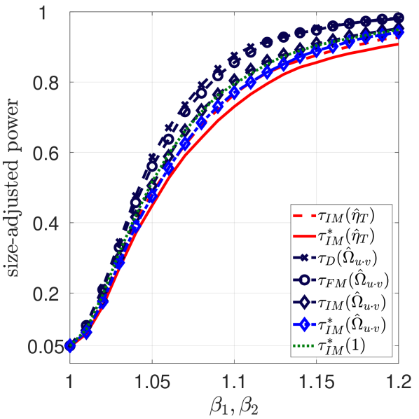
$T=100$, $\phi=0$

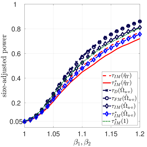
$T=100$, $\phi=0.9$

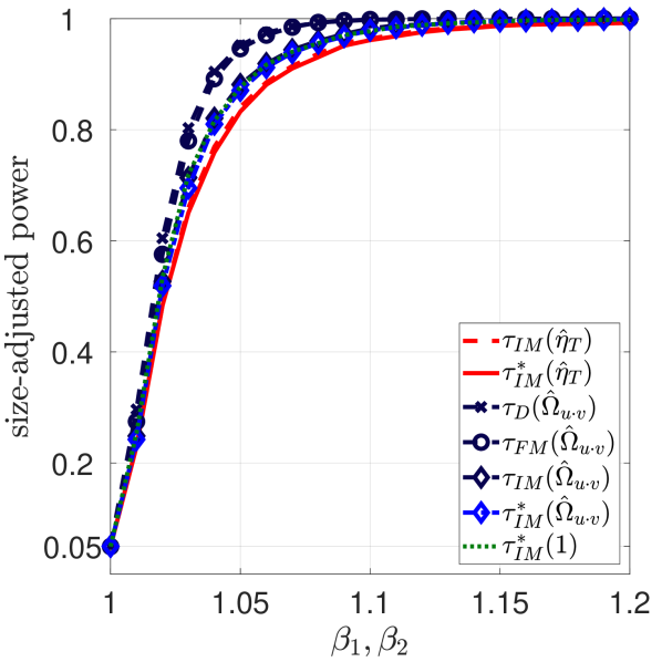
$T=250$, $\phi=0$

$T=250$, $\phi=0.9$

Figure 1: Size-adjusted power of the tests for $\text{H}_{0}:\beta_{1}=1,\ \beta_{2}=1$ at 5% level for $\rho_{1},\rho_{2}=0.6$. Notes: Superscript “$*$” signifies the use of bootstrap critical values. Whenever necessary, we use the Bartlett kernel to estimate long-run variance parameters.

6 Empirical Illustration: The Fisher Effect

In this section we briefly illustrate the usefulness of the self-normalized test developed in this paper in applications. Many empirical studies suggest that inflation and the short-term nominal interest rate do not cointegrate with the slope of inflation being equal to one, a finding at odds with the so-called Fisher effect that is backed by many theoretical models. The errors $u_{t}$ in the Fisher equation

$$i_{t}=\alpha+\beta\pi_{t}+u_{t},$$ (6.1)

$t=1,\ldots,T$, are likely to be highly persistent even in case cointegration between inflation $\pi_{t}$ and the short-term nominal interest rate $i_{t}$ prevails, [pp. 217]We08see, e. g.,. As demonstrated in our simulation study (and in many simulation studies before), highly persistent errors are well known to have adverse effects on the performance of estimators and tests in cointegrating regressions. Consequently, the Fisher effect might be rejected, even if it exists, solely due to the poor performance of the methods chosen by the applied researcher [for a detailed analysis of this phenomenon]CaPi04see. We08 shows that this problem can be tackled by using suitable panel methods, i. e., at the cost of including a large number of additional countries into the analysis. This may be undesirable for the applied researcher originally interested in analyzing the existence of the Fisher effect for a particular country only. Given its superior finite sample performance demonstrated in Section 5 compared to the traditional tests, the bootstrap-assisted self-normalized test developed in this paper seems to be useful to address this problem in the time series setting.

We investigate the validity of the Fisher effect for Germany and the United States between 1965Q1 and 2021Q1, using quarterly data ($T=225$) obtained from the OECD databases Economic Outlook and Main Economic Indicators. Before estimating (6.1) for both countries separately, we first assess whether the short-term interest rate and inflation are indeed non-stationary and cointegrated. To this end, we employ Br02’s Br02 self-normalized variance ratio unit root test and a Shin-type cointegration test based on the IM-OLS residuals allowing for a potentially non-zero mean. To estimate the long-run variance parameter required for the cointegration test, we use the Bartlett kernel and the corresponding data-dependent bandwidth selection rule of An91. All tests in this section are carried out at the nominal $10\%$ level. For both countries, the unit root test fails to reject the null hypothesis of non-stationarity of the interest rate and inflation and the cointegration test fails to reject the null hypothesis of cointegration between the two variables.

These preliminary results justify to estimate (6.1) on the individual country level using the IM-OLS estimator and to test whether $\beta$ is indeed equal to one using the bootstrap-assisted self-normalized test developed in this paper. We set the number of bootstrap replications to $1{,}499$ and determine the order of the VAR sieve as described in Section 5. For comparison, we also estimate (6.1) using the FM-OLS estimator and test unity of $\beta$ using the corresponding traditional Wald-type test. For the FM-OLS estimator and the test statistic based upon it we use the Bartlett kernel and the corresponding data-dependent bandwidth selection rule of An91 to estimate the long-run parameters. The results are reported in Table 2, which also presents the OLS estimates as a benchmark.

Estimates of $\beta$ Test statistics for $\text{H}_{0}:\beta=1$ Persistence Country OLS IM-OLS FM-OLS $\tau_{\scriptstyle\text{IM}}^{*}(\hat{\eta}_{T})$ $\tau_{\scriptstyle\text{FM}}(\hat{\Omega}_{u\cdot v})$ $\hat{\rho}_{1}$ Germany 1.36 1.68 1.53 26.72 (102.57) 2.85 (2.71) 0.92 United States 0.99 1.39 1.14 24.29 (102.32) 0.47 (2.71) 0.91 • Notes: All tests are carried out at the nominal $10\%$ level and reject the null hypothesis if the test statistic is larger than the corresponding critical value. Bootstrap critical values for the bootstrap-assisted self-normalized test $\tau_{\scriptstyle\text{IM}}^{*}(\hat{\eta}_{T})$ and chi-square critical values for the traditional test $\tau_{\scriptstyle\text{FM}}(\hat{\Omega}_{u\cdot v})$ in parenthesis. The measure of persistence $\hat{\rho}_{1}$ in the regression errors in (6.1) is obtained by regressing the OLS residuals on their first lag.

Table 2: Country specific results

The OLS estimate of $\beta$ is given by $1.36$ for Germany and $0.99$ for the United States, with the modified estimators yielding slightly larger estimates. The estimated values of $\beta$ compare well with the estimates obtained in [Table VII]We08 for the subperiod 1980Q1–2004Q4. To assess the persistence of the errors in (6.1), we regress the OLS residuals on their first lag. The resulting estimates of the AR(1) parameter are $0.92$ for Germany and $0.91$ for the United States, showing that the regression errors are indeed highly persistent. With respect to testing unity of $\beta$, Table 2 shows that the traditional FM-OLS based test accepts the hypothesized value of one for $\beta$ for the United States, but rejects the null hypothesis for Germany. In contrast, the bootstrap-assisted self-normalized test does not reject the hypothesis that $\beta$ is equal to one for both countries. Interestingly, the realizations of the self-normalized test statistic and the corresponding bootstrap critical values are very similar for Germany and the United States. This indicates that the validity of the Fisher effect is equally likely in both countries, although the estimates of $\beta$ are slightly closer to one for the United States. The traditional test thus gives misleading results.

Although our results show the importance of accounting for highly persistent regression errors, a more careful analysis is needed to assess the validity of the Fisher effect for the full period, as the link between inflation and the short-term interest rate might have weakened in the aftermath of the global financial crisis.

7 Conclusion

We propose a novel self-normalized test statistic for general linear restrictions in cointegrating regressions avoiding direct estimation of a long-run variance parameter. Its limiting null distribution is nonstandard, but we provide asymptotic critical values. Combining the self-normalization approach with a VAR sieve bootstrap to construct critical values further improves the performance of the self-normalized test in small to medium samples when the level of error serial correlation or regressor endogeneity is large. Constructing bootstrap critical values requires the choice of a single tuning parameter, the order of a VAR, which is a straightforward and well understood task in practice.

Simulation results and local asymptotic power analyses demonstrate that the bootstrap-assisted self-normalized test is considerably less prone to size distortions than the traditional tests at the cost of only small power losses. From a practical point of view, these small power losses are difficult to deem relevant in cointegrating regressions, given the enormous size improvements under the null hypothesis. An empirical application analyzing the validity of the Fisher effect in Germany and the United States exemplifies the advantage of the bootstrap-assisted self-normalized test over the traditional tests. Given that the bootstrap-assisted self-normalized test is easy to implement, we conclude that it should become a serious competitor to the traditional tests in practice.

Bootstrap-assisted self-normalized inference may also be a promising approach to address the enormous size distortions of hypothesis tests often observed in, e. g., cointegrated panels, cointegrating polynomial regressions and non-linear cointegrating regressions. We leave these interesting extensions for future research.

A Other Possible Choices for $\kappa$

Our particular choice for $\kappa$ in (3.10), the self-normalizer $\hat{\eta}_{T}$, is closely related to a seemingly natural kernel estimator of $\Omega_{u\cdot v}$ defined as

$$\widetilde{\Omega}_{u\cdot v}\left(\mathcal{K},b_{T}\right)\coloneqq T^{-1}\sum_{i=2}^{T}\sum_{j=2}^{T}\mathcal{K}\left(\frac{|i-j|}{b_{T}}\right)\Delta\hat{S}_{i}^{u}\Delta\hat{S}_{j}^{u},$$

where, as before, $\mathcal{K}(\cdot)$ is a kernel function and $b_{T}$ is a bandwidth parameter. In contrast to the traditional estimator $\hat{\Omega}_{u\cdot v}\left(\mathcal{K},b_{T}\right)$ defined in (3.12), $\widetilde{\Omega}_{u\cdot v}\left(\mathcal{K},b_{T}\right)$ is inconsistent for $\Omega_{u\cdot v}$ under common kernel and bandwidth assumptions. Nevertheless, $\widetilde{\Omega}_{u\cdot v}\left(\mathcal{K},b_{T}\right)$ serves as a useful starting point to motivate our choice of $\hat{\eta}_{T}$ as the self-normalizer.

We first note that under traditional kernel and bandwidth assumptions $\widetilde{\Omega}_{u\cdot v}\left(\mathcal{K},b_{T}\right)\overset{w}{\longrightarrow}\Omega_{u\cdot v}\left(1+\mathcal{Z}(2)^{\prime}\mathcal{Z}(2)\right)$, as $T\rightarrow\infty$, where $\mathcal{Z}(2)$ denotes the vector of the last $m$ components of the $2m$-dimensional vector $\mathcal{Z}$ defined in (3.3), see [Proof of Theorem 3]VoWa14. That is, the limiting distribution of $\widetilde{\Omega}_{u\cdot v}\left(\mathcal{K},b_{T}\right)$ is nuisance parameter free up to its scale-dependence on $\Omega_{u\cdot v}$, which leads to a nuisance parameter free limiting distribution of the test statistic $\tau_{\scriptstyle\text{IM}}(\widetilde{\Omega}_{u\cdot v}\left(\mathcal{K},b_{T}\right))$. However, $\widetilde{\Omega}_{u\cdot v}\left(\mathcal{K},b_{T}\right)$ is not a self-normalizer in the original sense, as its construction requires tuning parameter choices, which may have adverse effects on the performance of $\tau_{\scriptstyle\text{IM}}(\widetilde{\Omega}_{u\cdot v}\left(\mathcal{K},b_{T}\right))$ in finite samples. In particular, unreported preliminary simulation results indicate that $\widetilde{\Omega}_{u\cdot v}\left(\mathcal{K},b_{T}\right)$ is less successful in reducing the size distortions of the traditional test relative to $\hat{\eta}_{T}$.

In the special case where $\mathcal{K}\left(\cdot\right)$ is the Bartlett kernel ($\mathcal{K}_{\text{\scriptsize Bartlett}}$) and $b_{T}=T$, it follows from algebraic arguments used in [Proof of Lemma 1]CaSh06 in combination with similar arguments as used in the proof of Theorem 1 that

$$\widetilde{\Omega}_{u\cdot v}\left(\mathcal{K}_{\text{\scriptsize Bartlett}},T\right)=\hat{\eta}_{T}+T^{-2}\sum_{t=2}^{T}\left(\sum_{s=2}^{t}\Delta\hat{S}_{s}^{u}-\sum_{s=2}^{T}\Delta\hat{S}_{s}^{u}\right)^{2}$$

$$\overset{w}{\longrightarrow}\Omega_{u\cdot v}\left(\int_{0}^{1}\left(W_{u\cdot v}(r)-g(r)^{\prime}\mathcal{Z}\right)^{2}dr\right.$$

$$\hskip 56.9055pt\left.+\int_{0}^{1}\left([W_{u\cdot v}(r)-g(r)^{\prime}\mathcal{Z}]-[W_{u\cdot v}(1)-g(1)^{\prime}\mathcal{Z}]\right)^{2}dr\right),$$

as $T\rightarrow\infty$. The quantity $\widetilde{\Omega}_{u\cdot v}\left(\mathcal{K}_{\text{\scriptsize Bartlett}},T\right)$ is thus closely related to $\hat{\eta}_{T}$ and its limiting distribution is again nuisance parameter free up to its scale-dependence on $\Omega_{u\cdot v}$. Unreported preliminary simulation results show that $\tau_{\scriptstyle\text{IM}}(\widetilde{\Omega}_{u\cdot v}\left(\mathcal{K}_{\text{\scriptsize Bartlett}},T\right))$ performs similarly to $\tau_{\scriptstyle\text{IM}}(\hat{\eta}_{T})$ under the null hypothesis. However, $\tau_{\scriptstyle\text{IM}}(\widetilde{\Omega}_{u\cdot v}\left(\mathcal{K}_{\text{\scriptsize Bartlett}},T\right))$ has smaller (local asymptotic) power than $\tau_{\scriptstyle\text{IM}}(\hat{\eta}_{T})$ under the alternative.

Remark 5.

There is another interesting relation we want to highlight. If we assume for a moment that $\sum_{s=2}^{T}\Delta\hat{S}_{s}^{u}=\hat{S}_{T}^{u}-\hat{S}_{1}^{u}=0$, which does not hold in general, we obtain $\widetilde{\Omega}_{u\cdot v}\left(\mathcal{K}_{\text{\scriptsize Bartlett}},T\right)=2\hat{\eta}_{T}$. This relation fits well to the finding of KiVo02 in the stationary time series literature. The authors show that the self-normalization approach of KVB00 is exactly equivalent to using HAC standard errors based on the Bartlett kernel with bandwidth equal to sample size. From this perspective, choosing $\hat{\eta}_{T}$ as the self-normalizer seems to be the natural extension of the approach of KVB00 from the stationary time series literature to cointegrating regressions.

B Local Asymptotic Power

In this section we compare the asymptotic power properties of the self-normalized test $\tau_{\scriptstyle\text{IM}}(\hat{\eta}_{T})$ and the traditional test $\tau_{\scriptstyle\text{IM}}(\hat{\Omega}_{u\cdot v})$ under local alternatives. The results hold under Assumption 3, with $(y_{t})_{t=1}^{T}$ and $(x_{t})_{t=1}^{T}$ generated by (2.1) and (2.2), respectively. To ease exposition of the main arguments, we restrict attention to the single regressor case ($m=1$), which suffices to illustrate the main similarities and differences between the two tests. For $m=1$ the regression model becomes $y_{t}=x_{t}\beta+u_{t}$, with $\beta$ being a one-dimensional parameter. We are interested in testing the null hypothesis $\text{H}_{0}:\beta=\beta_{0}$. In this case, $\tau_{\scriptstyle\text{IM}}(\kappa)$ defined in (3.10) simplifies to

$$\tau_{\scriptstyle\text{IM}}(\kappa)=\left(\frac{\left(\hat{\beta}_{\scriptstyle\text{IM}}-\beta_{0}\right)}{\sqrt{\kappa\hat{V}_{T}(1,1)}}\right)^{2},$$ (B.1)

where $\hat{V}_{T}(1,1)$ denotes the upper-left element of the ($2\times 2$)-dimensional matrix $\hat{V}_{T}$ defined in (3.6). Straightforward calculations reveal that under the local alternative $\text{H}_{1}:\beta=\beta_{0}+c\,T^{-1}$, with $c\in{\mathbb{R}}$, the limiting distribution of $\tau_{\scriptstyle\text{IM}}(\hat{\Omega}_{u\cdot v})$ is given by

$$\tau_{\scriptstyle\text{IM}}(\hat{\Omega}_{u\cdot v})\overset{w}{\longrightarrow}\mathcal{G}_{c}\coloneqq\left(\frac{c\,\Omega_{vv}^{1/2}}{\Omega_{u\cdot v}^{1/2}\sqrt{\tilde{V}(1,1)}}+\frac{\mathcal{Z}(1)}{\sqrt{\tilde{V}(1,1)}}\right)^{2},$$ (B.2)

where $\tilde{V}(1,1)$ denotes the upper-left element of the nuisance parameter free ($2\times 2$)-dimensional matrix $\tilde{V}$ defined in (3.1) and $\mathcal{Z}(1)$ denotes the first element in the two-dimensional vector $\mathcal{Z}$ defined in (3.3). Analogously, the limiting distribution of $\tau_{\scriptstyle\text{IM}}(\hat{\eta}_{T})$ under the local alternative is given by

$$\tau_{\scriptstyle\text{IM}}(\hat{\eta}_{T}) \overset{w}{\longrightarrow}\mathcal{G}_{\scriptstyle\text{SN},c}\coloneqq\left(\frac{c\,\Omega_{vv}^{1/2}}{\Omega_{u\cdot v}^{1/2}\sqrt{\int_{0}^{1}\left(W_{u\cdot v}(r)-g(r)^{\prime}\mathcal{Z}\right)^{2}dr}\sqrt{\tilde{V}(1,1)}}\right.$$

$$\left.\hskip 85.35826pt+\frac{\mathcal{Z}(1)}{\sqrt{\int_{0}^{1}\left(W_{u\cdot v}(r)-g(r)^{\prime}\mathcal{Z}\right)^{2}dr}\sqrt{\tilde{V}(1,1)}}\right)^{2}.$$ (B.3)

Naturally, for $c=0$ the limiting distributions in (B.2) and (B) coincide with the chi-square distribution with one degree of freedom and the distribution $\mathcal{G}_{\scriptstyle\text{SN}}$ defined in (1), respectively. It follows that local asymptotic power of $\tau_{\scriptstyle\text{IM}}(\hat{\Omega}_{u\cdot v})$ at the nominal $5\%$ level is given by ${\mathbb{P}}\left(\mathcal{G}_{c}>\chi^{2}_{1,0.95}\right)$, where $\chi^{2}_{1,0.95}$ denotes the $0.95$-quantile of the chi-square distribution with one degree of freedom. Analogously, local asymptotic power of $\tau_{\scriptstyle\text{IM}}(\hat{\eta}_{T})$ at the nominal $5\%$ level is given by ${\mathbb{P}}\left(\mathcal{G}_{\scriptstyle\text{SN},c}>q_{1,1,0.95}\right)$, where $q_{1,1,0.95}$ denotes the corresponding $0.95$-quantile for the self-normalized test statistic given in Table D.4 in Online Appendix D ($56.58$; Panel A, $m=1$, $s=1$). Local asymptotic power of both tests depends on $c\,\Omega_{vv}^{1/2}\Omega_{u\cdot v}^{-1/2}$. For a given $c\neq 0$, local asymptotic power of the tests thus depends on both the long-run variance $\Omega_{vv}$ of the first differences $v_{t}=\Delta x_{t}$ of the regressor $x_{t}$ and the long-run variance $\Omega_{u\cdot v}$ of the regression error $u_{t}$ corrected for its conditional long-run mean given $v_{t}$. In particular, it follows from the definition of $\Omega_{u\cdot v}$ that local asymptotic power of the tests decreases as the variability in the regression errors increases. To assess the effect of the location parameter $c$, we plot the two power curves as a function of $c$ in Figure B.1 for fixed $\Omega_{vv}$ and $\Omega_{u\cdot v}$ using simulations. In particular, we set $\Omega_{vv}^{1/2}\Omega_{u\cdot v}^{-1/2}=1$ and approximate the stochastic terms using similar methods to those used to generate the critical values in Online Appendix D.

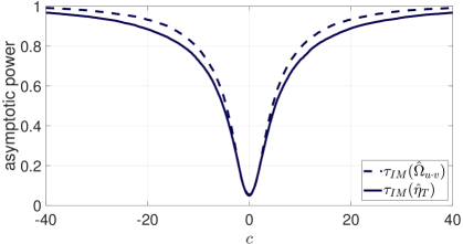
Figure B.1: Asymptotic power of the traditional test and the self-normalized test for $\text{H}_{0}:\beta=\beta_{0}$ under the local alternative $\beta=\beta_{0}+c\,T^{-1}$. Both tests are carried out at the nominal $5\%$ level.

Figure B.1 shows that both tests have asymptotic power against local alternatives, with local asymptotic power increasing symmetrically as $c$ moves away from zero. Local asymptotic power of the self-normalized test is similar to, but slightly below, local asymptotic power of the traditional Wald-type test. To quantify the local power loss, we consider two measures: the absolute local power loss, i. e., the difference in local power between the traditional test and the self-normalized test, and the relative local power loss, i. e., the absolute local power loss divided by local power of the traditional test. The largest absolute local power loss is about $0.06$ and occurs at around $c=\pm 10.6$, whereas the largest relative local power loss is about $10.3\%$ and occurs at around $c=\pm 5.1$. The results are consistent with the findings in the stationary time series literature, where local asymptotic power of self-normalized tests is well known to be often slightly below that of traditional tests, see, e. g., KVB00 and Sh15.

Remark 6.

Given the results in Theorem 3, it follows from consistency of the IM-OLS estimator of $\beta$ and imposing the null hypothesis when constructing the bootstrap data $y_{t}^{*}$ that the VAR sieve bootstrap is consistent for the limiting null distribution of the self-normalized test statistic even when the null hypothesis is incorrect. In the limit, the bootstrap critical value for the self-normalized test statistic thus coincides with the asymptotic critical value even under deviations from the null hypothesis. Consequently, local asymptotic power of the bootstrap-assisted self-normalized test coincides with local asymptotic power of the asymptotic version of the self-normalized test.

C Additional Finite Sample Results

C.1 Estimator Performance

We briefly compare the IM-OLS estimator with the D- and FM-OLS estimators in terms of bias and root mean squared error (RMSE). Implementing the D-OLS estimator requires choosing the numbers of leads and lags of the first differences of the integrated regressors. To this end, we use the Bayesian information criterion (BIC) analyzed in ChKu12, as it appears to be the most successful criterion – among those considered by the authors – in reducing the mean squared error of the D-OLS estimator. The FM-OLS estimator is based on an estimator of the long-run covariance matrix of $\{[u_{t},v_{t}^{\prime}]^{\prime}\}_{t\in{\mathbb{Z}}}$ as defined in (3.13). We analyze the results for the Bartlett kernel and the Quadratic Spectral (QS) kernel, together with the corresponding data-dependent bandwidth selection rules of An91. Table C.1 displays results for $\beta_{1}$. Although asymptotically unbiased, the D-, FM- and IM-OLS estimators are biased in finite samples. Generally, bias and RMSE increase in $\rho_{1},\rho_{2}$ and $\phi$ and decrease in $T$. In terms of bias the IM-OLS estimator performs similar to the D-OLS estimator and clearly outperforms the FM-OLS estimator. In terms of RMSE the results show that overall the D-OLS estimator performs best, followed by the FM-OLS estimator based on the Bartlett kernel. RMSE of the IM-OLS estimator is comparable to the RMSE of the FM-OLS estimator based on the QS kernel, which is often slightly larger than RMSE of the FM-OLS estimator based on the Bartlett kernel. We conclude that the IM-OLS estimator performs relatively well and serves as a good starting point for self-normalized inference in cointegrating regressions.

$\text{Bias}\times 100$ $\text{RMSE}\times 100$ FM-OLS FM-OLS $\phi$ $\rho_{1},\rho_{2}$ IM-OLS D-OLS Bartlett QS QML IM-OLS D-OLS Bartlett QS QML Panel A: $T=75$ $0$ 0 $-$0.25 $-$0.27 0.04 0.11 $-$0.05 5.15 3.52 3.28 3.42 15.31 0.3 $-$0.25 $-$0.08 0.66 0.79 $-$0.45 7.29 4.91 5.02 5.38 19.79 0.6 0.88 1.65 3.64 3.70 $-$6.82 12.72 11.68 11.12 11.97 374.48 0.9 19.63 12.69 24.93 25.00 $-$606.33 58.08 46.22 48.09 55.54 31796.03 $0.3$ 0 $-$0.28 $-$0.18 0.13 0.19 0.39 6.67 4.46 4.24 4.42 20.65 0.3 $-$0.28 0.10 0.87 1.00 0.42 9.46 7.43 6.50 6.93 23.56 0.6 0.91 1.52 4.16 4.30 1.25 16.45 16.59 13.63 14.75 77.59 0.9 20.44 12.89 26.44 26.37 75.50 68.99 58.15 54.10 88.03 6141.08 $0.9$ 0 $-$0.35 0.09 0.34 0.41 $-$0.66 9.74 8.06 6.27 6.56 20.00 0.3 $-$0.33 0.35 1.37 1.51 $-$0.95 13.83 12.87 9.56 10.16 76.13 0.6 0.96 1.60 5.14 5.59 $-$3.55 23.95 26.29 18.48 19.82 354.12 0.9 22.08 13.54 29.43 29.69 $-$31.68 92.30 83.42 66.97 122.62 4171.58 Panel B: $T=100$ $0$ 0 $-$0.07 $-$0.15 0.05 0.09 0.13 3.91 2.37 2.38 2.46 6.22 0.3 $-$0.03 0.03 0.45 0.51 $-$0.14 5.55 3.25 3.55 3.72 9.96 0.6 0.74 1.53 2.48 2.44 $-$2.05 9.71 6.63 7.76 8.25 115.53 0.9 14.76 11.97 20.06 20.35 $-$54.65 45.30 33.92 39.03 42.27 3497.87 $0.3$ 0 $-$0.07 $-$0.07 0.12 0.15 0.02 5.07 2.97 3.09 3.18 3.97 0.3 $-$0.01 0.19 0.60 0.65 0.09 7.20 4.21 4.62 4.84 11.40 0.6 0.83 1.71 2.92 2.94 $-$5.09 12.56 8.85 9.67 10.28 289.60 0.9 15.60 12.88 21.49 22.36 12.16 53.98 42.04 44.37 50.19 903.93 $0.9$ 0 $-$0.06 0.12 0.30 0.31 0.24 7.39 4.42 4.56 4.71 9.54 0.3 0.03 0.49 1.00 1.05 0.06 10.51 6.40 6.84 7.18 21.90 0.6 1.01 2.04 3.72 3.86 $-$1.24 18.27 13.33 13.42 14.37 168.09 0.9 17.27 14.19 24.28 25.81 123.50 72.40 58.58 55.89 66.60 4255.25 Panel C: $T=250$ $0$ 0 0.01 $-$0.06 0.02 0.02 0.01 1.59 0.91 0.91 0.92 0.95 0.3 0.03 0.02 0.12 0.12 0.01 2.27 1.25 1.33 1.35 1.38 0.6 0.21 0.46 0.79 0.69 0.04 3.96 2.38 2.80 2.84 2.50 0.9 5.01 4.25 8.83 8.67 $-$0.17 17.71 11.78 17.39 18.36 15.07 $0.3$ 0 0.02 $-$0.03 0.04 0.04 0.01 2.07 1.14 1.18 1.19 1.25 0.3 0.05 0.10 0.17 0.16 $-$0.00 2.95 1.61 1.74 1.77 1.83 0.6 0.24 0.55 0.93 0.84 0.01 5.14 3.06 3.54 3.63 3.33 0.9 5.32 4.98 9.64 9.82 $-$1.37 21.88 14.73 19.96 21.40 36.14 $0.9$ 0 0.04 0.08 0.09 0.09 0.02 3.02 1.67 1.74 1.77 1.91 0.3 0.07 0.25 0.30 0.29 0.07 4.30 2.41 2.58 2.65 2.87 0.6 0.31 0.75 1.21 1.15 0.03 7.50 4.44 5.01 5.19 6.09 0.9 5.95 6.43 11.20 11.85 5.25 30.54 20.66 25.18 27.23 290.19 Panel D: $T=500$ $0$ 0 0.01 $-$0.01 0.01 0.01 0.01 0.77 0.45 0.45 0.46 0.46 0.3 0.02 0.02 0.05 0.05 0.01 1.10 0.63 0.66 0.67 0.66 0.6 0.08 0.21 0.30 0.25 0.03 1.93 1.16 1.33 1.33 1.17 0.9 1.59 1.72 3.77 3.45 0.02 8.22 5.38 8.33 8.54 5.14 $0.3$ 0 0.02 $-$0.00 0.02 0.02 0.01 1.00 0.58 0.59 0.59 0.60 0.3 0.03 0.06 0.07 0.06 0.02 1.43 0.82 0.86 0.87 0.86 0.6 0.09 0.24 0.35 0.28 0.02 2.50 1.50 1.70 1.72 1.54 0.9 1.71 2.05 4.11 3.92 $-$0.07 10.41 6.82 9.64 10.07 6.86 $0.9$ 0 0.03 0.05 0.04 0.04 0.02 1.46 0.84 0.87 0.87 0.91 0.3 0.04 0.13 0.12 0.10 $-$0.01 2.09 1.21 1.28 1.29 1.33 0.6 0.12 0.31 0.45 0.39 $-$0.01 3.65 2.18 2.43 2.47 2.34 0.9 1.96 2.73 4.82 4.82 0.08 14.87 9.69 12.35 13.12 10.14 • Notes: The terms “Bartlett” and “QS” signify the kernel used to apply the FM-OLS estimator. QML denotes the quasi maximum likelihood estimator of Jo95, as described in Section C.3.

Table C.1: Bias and RMSE of various estimators of $\beta_{1}$

C.2 Results in the i.i.d. Innovations Case ($a_{1}=b_{1}=\rho_{3}=0$)

Traditional Wald-type tests Self-normalized tests Bartlett kernel QS kernel $\phi$ $\rho_{1},\rho_{2}$ $\tau_{\tiny\text{IM}}^{*}(1)$ $\tau_{\scriptstyle\text{IM}}(\hat{\eta}_{T})$ $\tau_{\scriptstyle\text{IM}}^{*}(\hat{\eta}_{T})$ $\tau_{\scriptstyle\text{D}}(\hat{\Omega}_{u\cdot v})$ $\tau_{\scriptstyle\text{FM}}(\hat{\Omega}_{u\cdot v})$ $\tau_{\scriptstyle\text{IM}}(\hat{\Omega}_{u\cdot v})$ $\tau_{\tiny\text{IM}}^{*}(\hat{\Omega}_{u\cdot v})$ $\tau_{\scriptstyle\text{D}}(\hat{\Omega}_{u\cdot v})$ $\tau_{\scriptstyle\text{FM}}(\hat{\Omega}_{u\cdot v})$ $\tau_{\scriptstyle\text{IM}}(\hat{\Omega}_{u\cdot v})$ $\tau_{\tiny\text{IM}}^{*}(\hat{\Omega}_{u\cdot v})$ Panel A: $T=75$ $0$ 0 0.09 0.03 0.07 0.16 0.16 0.11 0.07 0.19 0.20 0.14 0.06 0.3 0.11 0.05 0.07 0.20 0.20 0.14 0.07 0.20 0.23 0.15 0.06 0.6 0.15 0.09 0.08 0.34 0.35 0.23 0.09 0.34 0.37 0.22 0.08 0.9 0.48 0.35 0.19 0.72 0.79 0.66 0.25 0.79 0.84 0.73 0.26 $0.3$ 0 0.09 0.04 0.07 0.18 0.18 0.13 0.06 0.20 0.21 0.15 0.06 0.3 0.12 0.06 0.07 0.23 0.22 0.17 0.07 0.23 0.24 0.17 0.06 0.6 0.18 0.09 0.09 0.40 0.36 0.25 0.09 0.41 0.40 0.27 0.08 0.9 0.48 0.32 0.19 0.75 0.77 0.66 0.24 0.83 0.85 0.76 0.28 $0.9$ 0 0.16 0.05 0.10 0.23 0.20 0.15 0.09 0.24 0.22 0.16 0.08 0.3 0.19 0.06 0.10 0.32 0.26 0.19 0.11 0.33 0.29 0.21 0.09 0.6 0.26 0.10 0.12 0.48 0.38 0.29 0.13 0.53 0.45 0.34 0.11 0.9 0.51 0.30 0.19 0.78 0.74 0.68 0.25 0.88 0.87 0.82 0.28 Panel B: $T=100$ $0$ 0 0.08 0.03 0.07 0.13 0.14 0.10 0.06 0.15 0.17 0.12 0.06 0.3 0.09 0.05 0.07 0.16 0.18 0.14 0.07 0.15 0.18 0.13 0.06 0.6 0.13 0.08 0.07 0.27 0.31 0.19 0.08 0.26 0.31 0.18 0.07 0.9 0.39 0.27 0.14 0.66 0.73 0.57 0.18 0.72 0.79 0.64 0.20 $0.3$ 0 0.08 0.05 0.07 0.15 0.15 0.12 0.06 0.15 0.17 0.13 0.06 0.3 0.10 0.06 0.07 0.18 0.19 0.15 0.07 0.17 0.20 0.14 0.07 0.6 0.14 0.09 0.08 0.29 0.32 0.22 0.09 0.29 0.33 0.22 0.08 0.9 0.40 0.27 0.15 0.68 0.71 0.58 0.19 0.77 0.81 0.69 0.22 $0.9$ 0 0.13 0.05 0.08 0.17 0.17 0.13 0.08 0.16 0.18 0.14 0.07 0.3 0.15 0.06 0.09 0.21 0.22 0.17 0.09 0.21 0.24 0.17 0.09 0.6 0.21 0.09 0.10 0.32 0.33 0.25 0.11 0.35 0.37 0.28 0.09 0.9 0.43 0.25 0.16 0.69 0.69 0.59 0.21 0.81 0.84 0.74 0.23 Panel C: $T=250$ $0$ 0 0.06 0.04 0.06 0.08 0.09 0.07 0.06 0.09 0.10 0.08 0.05 0.3 0.07 0.05 0.06 0.10 0.12 0.09 0.06 0.09 0.11 0.09 0.06 0.6 0.07 0.06 0.06 0.17 0.19 0.11 0.06 0.15 0.17 0.10 0.06 0.9 0.18 0.13 0.07 0.38 0.52 0.28 0.09 0.40 0.55 0.31 0.09 $0.3$ 0 0.07 0.05 0.06 0.09 0.11 0.09 0.06 0.09 0.10 0.08 0.06 0.3 0.07 0.05 0.06 0.11 0.13 0.10 0.06 0.10 0.12 0.09 0.06 0.6 0.08 0.06 0.06 0.17 0.20 0.13 0.06 0.16 0.19 0.12 0.06 0.9 0.19 0.13 0.07 0.41 0.50 0.31 0.09 0.45 0.54 0.36 0.09 $0.9$ 0 0.08 0.05 0.06 0.10 0.12 0.09 0.07 0.09 0.11 0.09 0.07 0.3 0.10 0.05 0.07 0.12 0.15 0.11 0.07 0.11 0.14 0.10 0.07 0.6 0.12 0.07 0.07 0.17 0.21 0.15 0.07 0.17 0.21 0.14 0.07 0.9 0.23 0.14 0.09 0.43 0.48 0.35 0.11 0.50 0.57 0.42 0.11 Panel D: $T=500$ $0$ 0 0.05 0.04 0.05 0.07 0.07 0.07 0.05 0.07 0.07 0.07 0.05 0.3 0.05 0.05 0.05 0.08 0.08 0.08 0.05 0.07 0.08 0.07 0.05 0.6 0.06 0.05 0.05 0.11 0.13 0.09 0.05 0.10 0.11 0.08 0.05 0.9 0.08 0.06 0.05 0.20 0.34 0.13 0.05 0.20 0.35 0.14 0.05 $0.3$ 0 0.06 0.04 0.05 0.08 0.08 0.07 0.05 0.07 0.07 0.07 0.05 0.3 0.06 0.05 0.05 0.09 0.09 0.08 0.05 0.08 0.08 0.07 0.05 0.6 0.06 0.05 0.05 0.12 0.13 0.10 0.05 0.11 0.12 0.09 0.05 0.9 0.09 0.07 0.05 0.24 0.34 0.16 0.05 0.24 0.36 0.17 0.06 $0.9$ 0 0.07 0.04 0.05 0.08 0.08 0.08 0.06 0.07 0.08 0.07 0.06 0.3 0.07 0.05 0.05 0.09 0.10 0.09 0.06 0.08 0.10 0.08 0.05 0.6 0.08 0.05 0.05 0.13 0.14 0.11 0.06 0.12 0.13 0.10 0.06 0.9 0.12 0.08 0.06 0.28 0.33 0.20 0.06 0.30 0.36 0.21 0.06 • Notes: Superscript “$*$” signifies the use of bootstrap critical values. The asymptotic critical value for the self-normalized test $\tau_{\scriptstyle\text{IM}}(\hat{\eta}_{T})$ is given in Table D.4 in Online Appendix D ($167.23$; Panel A, $m=2$, $s=2$).

Table C.2: Empirical sizes of the tests for $\text{H}_{0}:\beta_{1}=1,\ \beta_{2}=1$ at $5\%$ level in the i.i.d. innovations case ($a_{1}=b_{1}=\rho_{3}=0$)

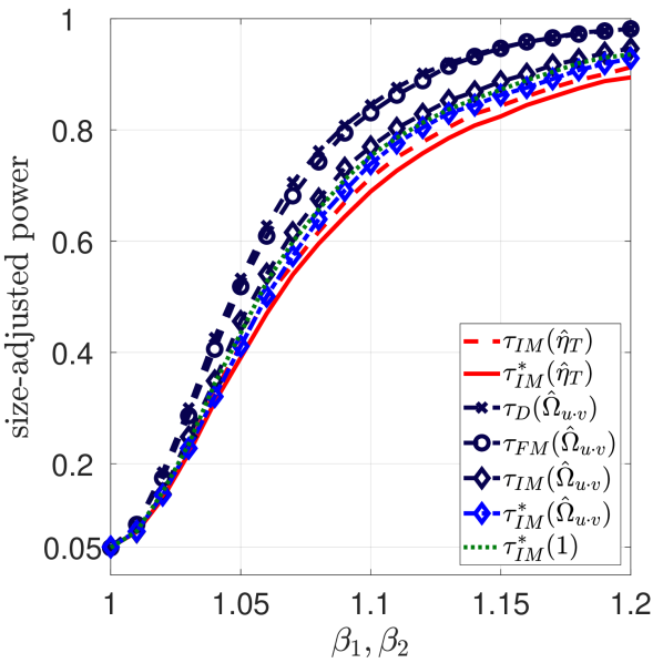
$T=100$, $\phi=0$

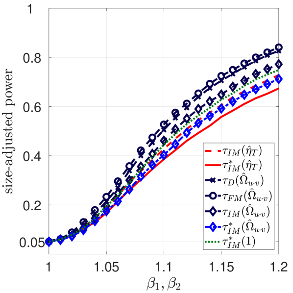
$T=100$, $\phi=0.9$

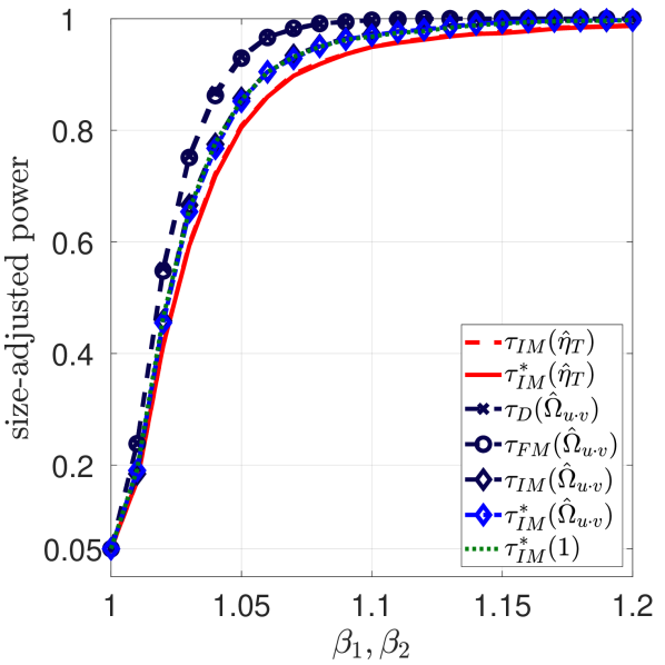
$T=250$, $\phi=0$

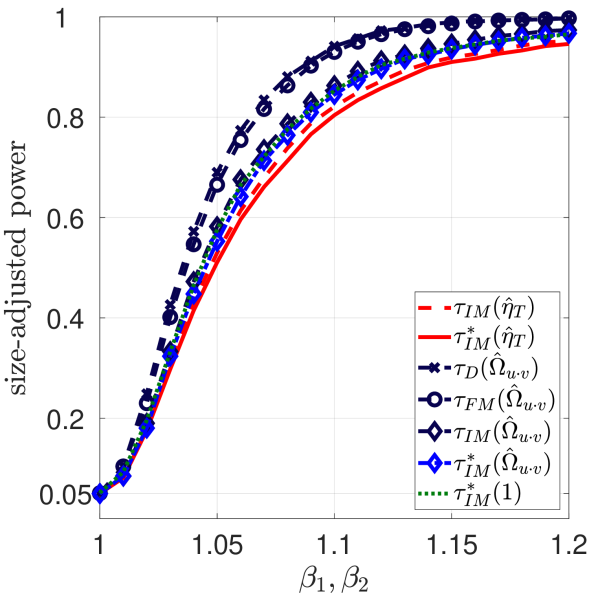
$T=250$, $\phi=0.9$

Figure C.2: Size-adjusted power of the tests for $\text{H}_{0}:\beta_{1}=1,\ \beta_{2}=1$ at 5% level for $\rho_{1},\rho_{2}=0.6$ in the i.i.d. innovations case ($a_{1}=b_{1}=\rho_{3}=0$). Notes: Superscript “$*$” signifies the use of bootstrap critical values. Whenever necessary, we use the Bartlett kernel to estimate long-run variance parameters.

C.3 Comparison with Johansen’s Likelihood Ratio Test

We can rewrite the data generating process (DGP) given in (5.1) and (5.2) as

$$\underbrace{\begin{bmatrix}1&-\beta_{1}&-\beta_{2}\\ 0&1&0\\ 0&0&1\end{bmatrix}}_{=:A_{0}}\begin{bmatrix}y_{t}\\ x_{1t}\\ x_{2t}\end{bmatrix}=\underbrace{\begin{bmatrix}0&0&0\\ 0&1&0\\ 0&0&1\end{bmatrix}}_{=:A_{1}}\begin{bmatrix}y_{t-1}\\ x_{1,t-1}\\ x_{2,t-1}\end{bmatrix}+\begin{bmatrix}u_{t}\\ v_{1t}\\ v_{2t}\end{bmatrix}\Leftrightarrow X_{t}=\Pi_{1}X_{t-1}+\epsilon_{t},$$

where $X_{t}\coloneqq[y_{t},x_{1t},x_{2t}]^{\prime}$, $\epsilon_{t}\coloneqq A_{0}^{-1}[u_{t},v_{1t},v_{2t}]^{\prime}$ and $\Pi_{1}\coloneqq A_{0}^{-1}A_{1}$. While the estimators and tests discussed so far ignore the exact characteristics of the DGP, the reduced rank quasi maximum likelihood (QML) estimator of Jo95 and the likelihood ratio (LR) test based upon it are tailor-made for this particular class of DGPs. Under this DGP, the performance of the parametric LR test thus serves as a natural benchmark for the performance of the non-parametric self-normalized test developed in this paper. To fix ideas, we consider the error correction model of order $k\geq 1$ with one cointegrated relation, i. e.,

$$\Delta X_{t}=ab^{\prime}X_{t-1}+\sum_{l=1}^{k-1}\Gamma_{l}\Delta X_{t-l}+\epsilon_{t},$$ (C.1)

where $\Delta X_{s}\coloneqq X_{s}-X_{s-1}$, $a=[-1,0,0]^{\prime}$ and $b=[1,-\beta_{1},-\beta_{2}]^{\prime}$. To test general linear hypotheses on the cointegration vector $b$, we first determine the order $k$ in (C.1) similarly as described in the beginning of Section 5 for the order of the VAR sieve. We then estimate the vector $b$ using the reduced rank QML estimator of Jo95. Testing the null hypothesis $\text{H}_{0}:\beta_{1}=1,\ \beta_{2}=1$ in (5.1) corresponds to testing the null hypothesis $\text{H}_{0}:b=[1,-1,-1]^{\prime}$ in (C.1). Under the null hypothesis, the LR test statistic of Jo95 is asymptotically chi-squared distributed with two degrees of freedom. CNR15 show how to replace the asymptotic chi-square critical values with bootstrap critical values to reduce the size distortions of the LR test in finite samples.

Before we compare the finite sample performance of the self-normalized test based on asymptotic critical values with the LR test based on asymptotic critical values and the bootstrap-assisted self-normalized test with the LR test based on bootstrap critical values generated as described in [p. 817]CNR15, we should mention one particular drawback of the reduced rank QML estimator. Table C.1 in Online Appendix C.1 shows that the QML estimator of $\beta_{1}$ has a very large bias for $\rho_{1},\rho_{2}=0.9$ and an extremely large RMSE for $\rho_{1},\rho_{2}\in\{0.6,0.9\}$ in small to medium samples. These results are in line with the findings in related literature, where the QML estimator is observed to occasionally produce estimates that are far away from the true parameter values, see, e. g., BrLu05 and references therein.

We now turn to the performance of the tests. Table C.3 displays the empirical sizes of both the LR test and the LR test based on bootstrap critical values ($\text{LR}^{*}$). Comparing empirical sizes of the LR test with those of the self-normalized test in Table 1, we note that that the self-normalized test based on asymptotic critical values clearly outperforms the LR test for almost all combinations of $T$, $\rho_{1},\rho_{2}$ and $\phi$. However, in case $\rho_{1},\rho_{2}=0.9$ and $\phi$ is smaller than $0.9$ size distortions of the self-normalized test are slightly larger than those of the LR test. In terms of size-adjusted power we note that the self-normalized test outperforms the LR test in small to medium samples or in case $\rho_{1},\rho_{2}=0.9$, see Figures C.3 and C.4.

Replacing asymptotic critical values with bootstrap critical values improves the performance of the LR test in small to medium samples considerably. Comparing the empirical sizes of $\text{LR}^{*}$ in Table C.3 with those of the bootstrap-assisted self-normalized test in Table 1 reveals that the two bootstrap tests perform similarly for all sample sizes considered, but $\text{LR}^{*}$ has slight performance advantages over the bootstrap-assisted self-normalized test in small to medium samples in case $\rho_{1},\rho_{2}=0.9$. However, this performance advantage of $\text{LR}^{*}$ over the bootstrap-assisted self-normalized test under the null hypothesis comes at the cost of some losses in size-adjusted power, as Figure C.4 reveals. In case $\rho_{1},\rho_{2}$ is large relative to the sample size, we observe that size-adjusted power of $\text{LR}^{*}$ is considerably smaller than size-adjusted power of the bootstrap-assisted self-normalized test. We also observe that the power difference between these tests can be much larger than the power difference between the bootstrap-assisted self-normalized test and the IM-OLS based Wald-type bootstrap test, compare Figure C.3 in case $T=100$, $\phi=0.9$ and $\rho_{1},\rho_{2}=0.6$ and Figure C.4 in case $T=75$, $\phi\in\{0,0.9\}$ and $\rho_{1},\rho_{2}=0.9$. For larger sample sizes, however, $\text{LR}^{*}$ has slightly larger size-adjusted power than the bootstrap-assisted self-normalized test and the IM-OLS based Wald-type bootstrap test, compare Figure C.3 in case $T=250$.

We conclude that the (bootstrap-assisted) self-normalized test performs well both under the null hypothesis and under the alternative even when compared to the parametric likelihood-ratio (bootstrap) test tailor made for the DGP under consideration. Therefore, in applications focusing on a particular cointegrating relation between the variables, the IM-OLS estimator and the (bootstrap-assisted) self-normalized test are a good alternative to the QML estimator and the likelihood-ration (bootstrap) test, especially when the QML estimator yields implausible estimates of the cointegrating vector.

$T=75$ $T=100$ $T=250$ $T=500$ $\phi$ $\rho_{1},\rho_{2}$ LR $\text{LR}^{*}$ LR $\text{LR}^{*}$ LR $\text{LR}^{*}$ LR $\text{LR}^{*}$ $0$ 0 0.13 0.06 0.10 0.06 0.07 0.06 0.07 0.06 0.3 0.14 0.06 0.11 0.06 0.08 0.06 0.07 0.06 0.6 0.16 0.07 0.13 0.06 0.09 0.06 0.07 0.06 0.9 0.27 0.08 0.20 0.07 0.11 0.07 0.08 0.06 $0.3$ 0 0.14 0.07 0.11 0.06 0.08 0.05 0.07 0.06 0.3 0.15 0.06 0.12 0.07 0.09 0.07 0.07 0.06 0.6 0.19 0.07 0.15 0.08 0.09 0.07 0.07 0.05 0.9 0.32 0.10 0.25 0.09 0.12 0.07 0.08 0.06 $0.9$ 0 0.18 0.09 0.14 0.08 0.09 0.07 0.07 0.06 0.3 0.20 0.08 0.15 0.08 0.10 0.06 0.07 0.06 0.6 0.23 0.09 0.18 0.07 0.10 0.06 0.09 0.07 0.9 0.39 0.09 0.31 0.09 0.14 0.07 0.12 0.08 • Note: Superscript “$*$” signifies the use of bootstrap critical values.

Table C.3: Empirical sizes of the LR test and the LR bootstrap test for $\text{H}_{0}:\beta_{1}=1,\ \beta_{2}=1$ at $5\%$ level

$T=100$, $\phi=0$

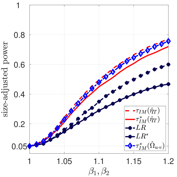
$T=100$, $\phi=0.9$

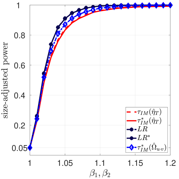
$T=250$, $\phi=0$

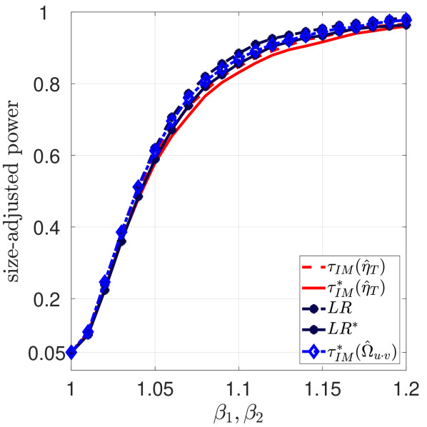
$T=250$, $\phi=0.9$

Figure C.3: Size-adjusted power of the tests for $\text{H}_{0}:\beta_{1}=1,\ \beta_{2}=1$ at 5% level for $\rho_{1},\rho_{2}=0.6$. Notes: Superscript “$*$” signifies the use of bootstrap critical values. Results for the (bootstrap-assisted) self-normalized test and the IM-OLS Wald-type bootstrap tests coincide with those in Figure 1.

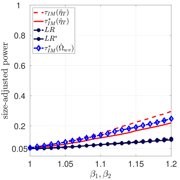
$T=75$, $\phi=0$

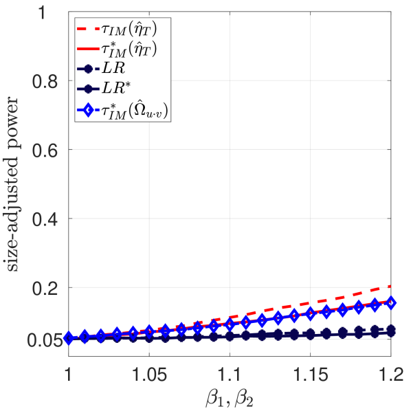
$T=75$, $\phi=0.9$

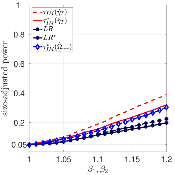
$T=100$, $\phi=0$

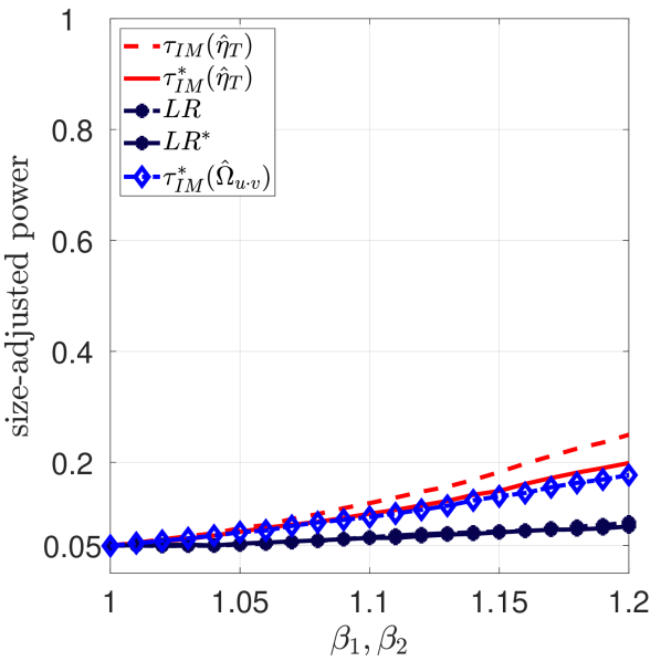
$T=100$, $\phi=0.9$

Figure C.4: Size-adjusted power of the tests for $\text{H}_{0}:\beta_{1}=1,\ \beta_{2}=1$ at 5% level for $\rho_{1},\rho_{2}=0.9$. Note: Superscript “$*$” signifies the use of bootstrap critical values. Results for the IM-OLS based Wald-type bootstrap test are based on the Bartlett kernel.

D Asymptotic Critical Values

To simulate asymptotically valid critical values, we approximate standard Brownian motions with normalized sums of $10{,}000$ i.i.d. standard normal random variables and approximate the corresponding integrals accordingly. The fact that the numerator of the limiting null distribution of the self-normalized test statistic given in (1) is invariant to $\Pi$ and only depends on the number of linearly independent restrictions under the null hypothesis justifies to set $\Pi=I_{2m}$ and $R_{2}=[I_{s},0_{s\times(2m-s)}]$. We tabulate critical values based on $10{,}000$ replications for various choices of $m$ and $s$ and different deterministic regressors in (2.1) in Table D.4.

$m=1$ $m=2$ $m=3$ $m=4$ $\%$ $s=1$ $s=1$ $s=2$ $s=1$ $s=2$ $s=3$ $s=1$ $s=2$ $s=3$ $s=4$ Panel A: No deterministic regressors 90.0 36.63 66.33 122.32 94.04 172.00 240.58 131.68 232.77 318.25 402.61 95.0 56.58 96.51 167.23 140.69 231.79 313.46 189.15 309.06 407.17 510.60 97.5 79.24 131.79 216.99 191.68 290.47 390.38 256.38 390.07 504.08 630.19 99.0 120.10 189.69 286.97 266.16 375.30 494.00 355.25 505.21 645.89 767.61 Panel B: Intercept ($d_{t}=1$) 90.0 64.13 94.15 168.58 126.65 221.45 305.36 162.08 278.05 382.30 481.15 95.0 95.81 140.55 233.15 187.03 297.11 396.56 236.54 372.79 487.71 596.15 97.5 136.10 190.23 292.64 245.93 375.55 488.35 325.56 458.37 587.85 720.31 99.0 187.13 263.92 381.78 338.59 474.31 602.27 421.68 582.89 719.98 872.07 Panel C: Intercept and linear time trend ($d_{t}=[1,t]^{\prime}$) 90.0 90.44 122.19 209.54 152.66 261.47 363.17 180.25 311.22 434.29 545.37 95.0 134.19 171.46 283.33 219.51 354.08 460.37 258.75 423.39 546.31 688.21 97.5 183.51 231.09 357.66 294.26 433.33 569.84 342.56 524.25 686.44 810.09 99.0 243.72 304.08 460.98 409.03 556.42 713.24 478.05 680.76 821.12 977.09 Panel D: Intercept, linear and square time trend ($d_{t}=[1,t,t^{2}]^{\prime}$) 90.0 115.13 138.49 245.91 175.40 302.95 418.77 205.72 352.96 479.57 608.35 95.0 166.35 200.65 331.26 255.74 402.90 530.94 303.58 465.28 621.70 764.20 97.5 217.42 268.86 401.63 348.51 509.51 637.29 390.59 589.05 762.57 902.89 99.0 290.63 357.58 513.85 472.49 646.48 800.81 527.20 754.26 923.59 1070.32 Panel E: Intercept, linear, square and cubic time trend ($d_{t}=[1,t,t^{2},t^{3}]^{\prime}$) 90.0 137.70 166.87 292.13 197.84 340.61 465.58 229.38 392.80 533.60 680.84 95.0 198.48 237.82 379.15 288.65 446.27 590.05 334.55 509.11 684.33 858.04 97.5 263.30 308.64 467.71 391.70 565.65 720.19 438.56 645.41 853.07 1004.50 99.0 352.56 406.48 587.03 539.71 726.07 903.53 592.44 846.82 1052.20 1222.78 • Notes: $s$ is the number of linearly independent restrictions under the null hypothesis on the coefficients corresponding to the $m\geq s$ integrated regressors.

Table D.4: Asymptotic critical values for $\tau_{\scriptstyle\text{IM}}(\hat{\eta}_{T})$

E Proofs of Main Results

Proof of Theorem 1. [Lemma 2]VoWa14 show that

$$T^{-1/2}\sum_{t=2}^{\lfloor rT\rfloor}\Delta\hat{S}_{t}^{u}\overset{w}{\longrightarrow}\Omega_{u\cdot v}^{1/2}\left(W_{u\cdot v}(r)-g(r)^{\prime}\mathcal{Z}\right),\quad 0\leq r\leq 1,$$

as $T\rightarrow\infty$. The continuous mapping theorem thus yields

$$\hat{\eta}_{T}=T^{-1}\sum_{t=2}^{T}\left(T^{-1/2}\sum_{s=2}^{t}\Delta\hat{S}_{s}^{u}\right)^{2}\overset{w}{\longrightarrow}\Omega_{u\cdot v}\int_{0}^{1}\left(W_{u\cdot v}(r)-g(r)^{\prime}\mathcal{Z}\right)^{2}dr,$$

as $T\rightarrow\infty$. The final result now follows with standard arguments from (3.9). $\square$

The proof of the remaining results relies on the following lemma.

Lemma 1.

Under Assumptions 1, 2 and 4, it holds that

$$\max_{q+1\leq t\leq T}|\hat{w}_{t}-w_{t}|_{F}=O_{\mathbb{P}}(T^{-1/2})$$ (E.1)

and

$$q^{1/2}\sum_{j=1}^{q}|\hat{\Phi}_{j}(q)-\tilde{\Phi}_{j}(q)|_{F}=O_{\mathbb{P}}(q^{3}/T)=o_{\mathbb{P}}(1),$$ (E.2)

where $\tilde{\Phi}_{1}(q),\ldots,\tilde{\Phi}_{q}(q)$ denote the solution of the sample Yule-Walker equations in the regression of $w_{t}$ on $w_{t-1},\ldots,w_{t-q}$, $t=q+1,\ldots,T$.

Proof.

We provide a proof in Online Appendix F. ∎

Two key ingredients in the proof of Lemma 1, which are also useful hereafter, are the following: First, it holds under Assumptions 1 and 4 that

$$q^{3/2}\sup_{1\leq j\leq q}|\tilde{\Phi}_{j}(q)-\Phi_{j}(q)|_{F}=q^{3/2}O_{\mathbb{P}}((\ln(T)/T)^{1/2})=O_{\mathbb{P}}(1),$$ (E.3)

compare [Remark 3.3.]MeKr15, where $\Phi_{1}(q),\ldots,\Phi_{q}(q)$ denote the finite predictor coefficients, i. e., the solution of the population Yule-Walker equations based on the true moments. Second, under Assumption 1 with $k\geq 3/2$, there exist constants $q_{0}\in{\mathbb{N}}$ and $c<\infty$ such that

$$\sum_{j=1}^{q}(1+j)^{k}|\Phi_{j}(q)-\Phi_{j}|_{F}\leq c\sum_{j=q+1}^{\infty}(1+j)^{k}|\Phi_{j}|_{F},$$ (E.4)

for all $q\geq q_{0}$ and the right-hand side converges to zero as $q\rightarrow\infty$, see [Lemma 3.1]MeKr15.

We use Lemma 1 to prove the following two lemmas. Subsequently, we use the following two lemmas to prove Proposition 1.

Lemma 2.

It holds under Assumptions 1 and 4 that

$${\mathbb{E}}^{*}\left(|\varepsilon_{t}^{*}|_{F}^{a}\right)=(T-q)^{-1}\sum_{t=q+1}^{T}|\hat{}\varepsilon_{t}(q)-\bar{\hat{\varepsilon}}_{T}(q)|_{F}^{a}=O_{\mathbb{P}}(1),$$

in ${\mathbb{P}}$, for the $a>2$ from Assumption 1.

Proof.

We provide a proof in Online Appendix F. ∎

Lemma 3.

It holds under Assumptions 1, 2 and 4 that

$${\mathbb{E}}^{*}\left(\varepsilon_{t}^{*}\varepsilon_{t}^{*\prime}\right)=(T-q)^{-1}\sum_{t=q+1}^{T}\left(\hat{}\varepsilon_{t}(q)-\bar{\hat{\varepsilon}}_{T}(q)\right)\left(\hat{}\varepsilon_{t}(q)-\bar{\hat{\varepsilon}}_{T}(q)\right)^{\prime}=\Sigma+o_{\mathbb{P}}(1),$$

in ${\mathbb{P}}$.

Proof.

We provide a proof in Online Appendix F. ∎

Proof of Proposition 1. Given Lemma 2 and Lemma 3, the result follows immediately from Ei87, as in [p. 714]CPS06. $\square$

Proof of Theorem 2. Using similar arguments as [p. 670]PSU10, it follows that

$$B_{T}^{*}(r)=T^{-1/2}\sum_{t=1}^{\lfloor rT\rfloor}w_{t}^{*}=\left(I-\sum_{j=1}^{q}\hat{\Phi}_{j}(q)\right)^{-1}W_{T}^{*}(r)+T^{-1/2}(\bar{w}_{0}^{*}-\bar{w}_{\lfloor rT\rfloor}^{*}),$$

where $\bar{w}_{t-1}^{*}\coloneqq\left(I-\sum_{j=1}^{q}\hat{\Phi}_{j}(q)\right)^{-1}\sum_{i=1}^{q}\left(\sum_{j=i}^{q}\hat{\Phi}_{j}(q)\right)w_{t-i}^{*}$. It thus remains to show that

$$I-\sum_{j=1}^{q}\hat{\Phi}_{j}(q)\overset{p}{\longrightarrow}\Phi(1)$$ (E.5)

and

$${\mathbb{P}}^{*}\left(\max_{0\leq t\leq T}|T^{-1/2}\bar{w}_{t}^{*}|_{F}>\delta\right)=o_{\mathbb{P}}(1).$$ (E.6)

We first show (E.5). From Lemma 1, (E.3) and (E.4), we obtain

$$|I-\sum_{j=1}^{q}\hat{\Phi}_{j}(q)-\Phi(1)|_{F} \leq\sum_{j=1}^{q}|\hat{\Phi}_{j}(q)-\tilde{\Phi}_{j}(q)|_{F}+\sum_{j=1}^{q}|\tilde{\Phi}_{j}(q)-\Phi_{j}(q)|_{F}$$

$$\quad+\sum_{j=1}^{q}|\Phi_{j}(q)-\Phi_{j}|_{F}+\sum_{j=q+1}^{\infty}|\Phi_{j}|_{F}$$

$$\leq\sum_{j=1}^{q}|\hat{\Phi}_{j}(q)-\tilde{\Phi}_{j}(q)|_{F}+q\sup_{1\leq j\leq q}|\tilde{\Phi}_{j}(q)-\Phi_{j}(q)|_{F}$$

$$\quad+c\sum_{j=q+1}^{\infty}|\Phi_{j}|_{F}+\sum_{j=q+1}^{\infty}|\Phi_{j}|_{F}$$

$$=o_{\mathbb{P}}(1)+o_{\mathbb{P}}(1)+o(1)+o(1)=o_{\mathbb{P}}(1).$$

To prove (E.6), we note that it follows from strict stationarity of $\{\bar{w}_{t}^{*}\}_{t\in{\mathbb{Z}}}$ and Markov’s inequality, that

$${\mathbb{P}}^{*}\left(\max_{0\leq t\leq T}|T^{-1/2}\bar{w}_{t}^{*}|_{F}>\delta\right) \leq\sum_{t=0}^{T}{\mathbb{P}}^{*}\left(|T^{-1/2}\bar{w}_{t}^{*}|_{F}>\delta\right)$$

$$\leq(T+1){\mathbb{P}}^{*}\left(|T^{-1/2}\bar{w}_{t}^{*}|_{F}>\delta\right)$$

$$\leq\delta^{-a}(T^{1-a/2}+T^{-a/2}){\mathbb{E}}^{*}\left(|\bar{w}_{t}^{*}|_{F}^{a}\right),$$

with the $a>2$ from Assumption 1, compare [p. 486]Pa02. Similarly as in [p. 671]PSU10, we obtain

$${\mathbb{E}}^{*}\left(|\bar{w}_{t}^{*}|_{F}^{a}\right)\leq c\left(m+1\right)^{a/2-1}\left(\sum_{j=0}^{\infty}|\bar{\hat{\Psi}}_{j}(q)|_{F}^{2}\right)^{a/2}{\mathbb{E}}^{*}\left(|\varepsilon_{t}^{*}|_{F}^{a}\right),$$

for some constant $c$ and $\bar{\hat{\Psi}}_{j}(q)\coloneqq\sum_{i=j+1}^{\infty}\hat{\Psi}_{i}(q)$, where the matrices $\hat{\Psi}_{j}$ are determined by the power series expansion of the inverse of $I-\sum_{j=1}^{q}\hat{\Phi}_{j}(q)z^{j}$. As discussed in [p. 671]PSU10 it follows that $\sum_{j=0}^{\infty}|\bar{\hat{\Psi}}_{j}(q)|_{F}^{2}=O_{\mathbb{P}}(1)$ if we can show that $\sum_{j=1}^{q}j^{1/2}|\hat{\Psi}_{j}(q)|_{F}=O_{\mathbb{P}}(1)$, which in turn holds if $\sum_{j=1}^{q}j^{1/2}|\hat{\Phi}_{j}(q)|_{F}=O_{\mathbb{P}}(1)$. Using again Lemma 1, (E.3) and (E.4), we obtain

$$\sum_{j=1}^{q}j^{1/2}|\hat{\Phi}_{j}(q)|_{F} \leq\sum_{j=1}^{q}j^{1/2}|\hat{\Phi}_{j}(q)-\tilde{\Phi}_{j}(q)|_{F}+\sum_{j=1}^{q}j^{1/2}|\tilde{\Phi}_{j}(q)-\Phi_{j}(q)|_{F}$$

$$\quad+\sum_{j=1}^{q}j^{1/2}|\Phi_{j}(q)-\Phi_{j}|_{F}+\sum_{j=1}^{q}j^{1/2}|\Phi_{j}|_{F}$$

$$\leq q^{1/2}\sum_{j=1}^{q}|\hat{\Phi}_{j}(q)-\tilde{\Phi}_{j}(q)|_{F}+q^{1/2}\sum_{j=1}^{q}|\tilde{\Phi}_{j}(q)-\Phi_{j}(q)|_{F}$$

$$\quad+\sum_{j=1}^{q}(1+j)|\Phi_{j}(q)-\Phi_{j}|_{F}+\sum_{j=1}^{q}j^{1/2}|\Phi_{j}|_{F}$$

$$\leq q^{1/2}\sum_{j=1}^{q}|\hat{\Phi}_{j}(q)-\tilde{\Phi}_{j}(q)|_{F}+q^{3/2}\sup_{1\leq j\leq q}|\tilde{\Phi}_{j}(q)-\Phi_{j}(q)|_{F}$$

$$\quad+\sum_{j=1}^{q}(1+j)|\Phi_{j}(q)-\Phi_{j}|_{F}+\sum_{j=1}^{q}j^{1/2}|\Phi_{j}|_{F}$$

$$=o_{\mathbb{P}}(1)+O_{\mathbb{P}}(1)+o(1)+O(1)=O_{\mathbb{P}}(1).$$

This completes the proof, since ${\mathbb{E}}^{*}\left(|\varepsilon_{t}^{*}|_{F}^{a}\right)=O_{\mathbb{P}}(1)$ by Lemma 2 for the $a>2$ from Assumption 1.  $\square$

Proof of Theorem 3. The first result in Theorem 3 follows from the bootstrap invariance principle result in Theorem 2 and similar arguments as used in [Proof of Theorem 2]VoWa14. The second result then follows from the bootstrap invariance principle and similar arguments as used in the proof of Theorem 1.  $\square$

F Proofs of Auxiliary Results

Proof of Lemma 1. The solution of the sample Yule-Walker equations in the regression of $w_{t}$ on $w_{t-1},\ldots,w_{t-q}$, $t=q+1,\ldots,T$, can be written in compact form as a ($(m+1)\times q(m+1)$)-dimensional matrix

$$\boldsymbol{\tilde{\Phi}}(q)\coloneqq[\tilde{\Phi}_{1}(q),\ldots,\tilde{\Phi}_{q}(q)]=\tilde{\Gamma}\tilde{G}^{-1},$$

with the ($(m+1)\times q(m+1)$)-dimensional matrix $\tilde{\Gamma}\coloneqq\left[\tilde{\Gamma}(1),\ldots,\tilde{\Gamma}(q)\right]$, the ($q(m+1)\times q(m+1)$)-dimensional matrix $\tilde{G}\coloneqq\left(\tilde{\Gamma}(s-r)\right)_{r,s=1,\ldots,q}$ and the ($(m+1)\times(m+1)$)-dimensional empirical autocovariance matrix of $w_{1},\ldots,w_{T}$ at lag $-q+1\leq h\leq q$, given by

$$\tilde{\Gamma}(h)\coloneqq T^{-1}\sum_{t=\max\{1,1-h\}}^{\min\{T,T-h\}}(w_{t+h}-\bar{w}_{T})(w_{t}-\bar{w}_{T})^{\prime},$$

where $\bar{w}_{T}\coloneqq T^{-1}\sum_{t=1}^{T}w_{t}$. Analogously, the solution of the sample Yule-Walker equations in the regression of $\hat{w}_{t}$ on $\hat{w}_{t-1},\ldots,\hat{w}_{t-q}$, $t=q+1,\ldots,T$, can be written in compact form as

$$\boldsymbol{\hat{\Phi}}(q)\coloneqq[\hat{\Phi}_{1}(q),\ldots,\hat{\Phi}_{q}(q)]=\hat{\Gamma}\hat{G}^{-1},$$

with $\hat{\Gamma}\coloneqq\left[\hat{\Gamma}(1),\ldots,\hat{\Gamma}(q)\right]$, $\hat{G}\coloneqq\left(\hat{\Gamma}(s-r)\right)_{r,s=1,\ldots,q}$ and $\hat{\Gamma}(h)$ the empirical autocovariance matrix of $\hat{w}_{1},\ldots,\hat{w}_{T}$ at lag $-q+1\leq h\leq q$. Taking the difference of $\boldsymbol{\tilde{\Phi}}(q)$ and $\boldsymbol{\hat{\Phi}}(q)$, adding and subtracting $\hat{\Gamma}\tilde{G}^{-1}$ and using

$$\tilde{G}^{-1}-\hat{G}^{-1}=\tilde{G}^{-1}(\hat{G}-\tilde{G})\hat{G}^{-1}$$

leads to

$$\boldsymbol{\hat{\Phi}}(q)-\boldsymbol{\tilde{\Phi}}(q)=\hat{\Gamma}\tilde{G}^{-1}(\tilde{G}-\hat{G})\hat{G}^{-1}-(\tilde{\Gamma}-\hat{\Gamma})\tilde{G}^{-1}$$

Hence, we have to consider $\tilde{G}-\hat{G}$ in more detail ($\tilde{\Gamma}-\hat{\Gamma}$ works similarly). A typical block element of $\tilde{G}-\hat{G}$ is

$$\tilde{\Gamma}(h)-\hat{\Gamma}(h) =T^{-1}\sum_{t=\max\{1,1-h\}}^{\min\{T,T-h\}}(w_{t+h}-\bar{w}_{T})(w_{t}-\bar{w}_{T})^{\prime}$$

$$\quad-T^{-1}\sum_{t=\max\{1,1-h\}}^{\min\{T,T-h\}}(\hat{w}_{t+h}-\bar{\hat{w}}_{T})(\hat{w}_{t}-\bar{\hat{w}}_{T})^{\prime}$$

$$=T^{-1}\sum_{t=\max\{1,1-h\}}^{\min\{T,T-h\}}(w_{t+h}-\bar{w}_{T})(w_{t}-\hat{w}_{t}-(\bar{w}_{T}-\bar{\hat{w}}_{T}))^{\prime}$$

$$\quad-T^{-1}\sum_{t=\max\{1,1-h\}}^{\min\{T,T-h\}}(\hat{w}_{t+h}-w_{t+h}-(\bar{\hat{w}}_{T}-\bar{w}_{T}))(\hat{w}_{t}-\bar{\hat{w}}_{T})^{\prime}$$

$$=A_{1}(h)-A_{2}(h),$$

with an obvious definition for $A_{1}(h)$ and $A_{2}(h)$. Let us consider $A_{1}(h)$ in more detail ($A_{2}(h)$ works similarly). Using $\hat{w}_{t}=[\hat{u}_{t},v_{t}^{\prime}]^{\prime}$ and $\hat{u}_{t}=y_{t}-x_{t}^{\prime}\hat{\beta}_{\scriptstyle\text{IM}}$ together with the model equations (2.1) and (2.2), we get

$$w_{t}-\hat{w}_{t}=\begin{bmatrix}u_{t}-\hat{u}_{t}\\ 0_{m\times 1}\end{bmatrix}=\begin{bmatrix}y_{t}-x_{t}^{\prime}\beta-(y_{t}-x_{t}^{\prime}\hat{\beta}_{\scriptstyle\text{IM}})\\ 0_{m\times 1}\end{bmatrix}=\begin{bmatrix}x_{t}^{\prime}(\hat{\beta}_{\scriptstyle\text{IM}}-\beta)\\ 0_{m\times 1}\end{bmatrix}.$$ (F.1)

Before we continue, note that the last equality implies

$$\max_{1\leq t\leq T}|\hat{w}_{t}-w_{t}|_{F}\leq T^{-1/2}\max_{1\leq t\leq T}|T^{-1/2}x_{t}|_{F}|T\left(\hat{\beta}_{\scriptstyle\text{IM}}-\beta\right)|_{F}=O_{\mathbb{P}}(T^{-1/2}),$$

since $\max_{1\leq t\leq T}|T^{-1/2}x_{t}|_{F}=\sup_{0\leq r\leq 1}|T^{-1/2}x_{\lfloor rT\rfloor}|_{F}$ converges by Assumption 3 and the continuous mapping theorem to $\sup_{0\leq r\leq 1}|B_{v}(r)|_{F}=O_{\mathbb{P}}(1)$ and $\hat{\beta}_{\scriptstyle\text{IM}}$ is rate-$T$ consistent. This proves (E.1).

We now proceed with the proof of (E.2). From (F.1) we obtain

$$A_{1}(h) =T^{-1}\sum_{t=\max\{1,1-h\}}^{\min\{T,T-h\}}(w_{t+h}-\bar{w}_{T})\begin{bmatrix}(x_{t}-\bar{x}_{T})^{\prime}(\hat{\beta}_{\scriptstyle\text{IM}}-\beta)\\ 0_{m\times 1}\end{bmatrix}^{\prime}$$

$$=T^{-1}\sum_{t=\max\{1,1-h\}}^{\min\{T,T-h\}}(w_{t+h}-\bar{w}_{T})[(x_{t}-\bar{x}_{T})^{\prime}(\hat{\beta}_{\scriptstyle\text{IM}}-\beta),0_{1\times m}]$$

$$=\tilde{\Gamma}_{w,x}(h)(\hat{\beta}_{\scriptstyle\text{IM}}-\beta)e_{1}^{\prime},$$

where $\tilde{\Gamma}_{w,x}(h)\coloneqq T^{-1}\sum_{t=\max\{1,1-h\}}^{\min\{T,T-h\}}(w_{t+h}-\bar{w}_{T})(x_{t}-\bar{x}_{T})^{\prime}$ is ($(m+1)\times m$)-dimensional and $e_{1}\coloneqq(1,0_{1\times m})^{\prime}$ is the first $(m+1)$-dimensional unit vector. Denoting the part of $\tilde{G}-\hat{G}$ that consists of block-entries $A_{1}(h)$ by $\tilde{G}_{1}-\hat{G}_{1}$, we get

$$\tilde{G}_{1}-\hat{G}_{1}=\begin{bmatrix}\tilde{\Gamma}_{w,x}(s-r)(\hat{\beta}_{\scriptstyle\text{IM}}-\beta)e_{1}^{\prime}\end{bmatrix}_{r,s=1,\ldots,q}=\tilde{\Gamma}_{w,x}(I_{q}\otimes((\hat{\beta}_{\scriptstyle\text{IM}}-\beta)e_{1}^{\prime})),$$

where $\tilde{\Gamma}_{w,x}\coloneqq(\tilde{\Gamma}_{w,x}(s-r))_{r,s=1,\ldots,q}$ is ($q(m+1)\times qm$)-dimensional. For the second factor we have

$$|I_{q}\otimes((\hat{\beta}_{\scriptstyle\text{IM}}-\beta)e_{1}^{\prime})|_{F} =\sqrt{\text{tr}\left((I_{q}\otimes((\hat{\beta}_{\scriptstyle\text{IM}}-\beta)e_{1}^{\prime}))^{\prime}I_{q}\otimes((\hat{\beta}_{\scriptstyle\text{IM}}-\beta)e_{1}^{\prime})\right)}$$

$$=\sqrt{\text{tr}\left(I_{q}\otimes(e_{1}(\hat{\beta}_{\scriptstyle\text{IM}}-\beta)^{\prime}(\hat{\beta}_{\scriptstyle\text{IM}}-\beta)e_{1}^{\prime}\right))}$$

$$=\sqrt{\text{tr}\left(I_{q}\otimes\text{diag}\left(\sum_{i=1}^{m}(\hat{\beta}_{\scriptstyle\text{IM},i}-\beta_{i})^{2},0,\ldots,0\right)\right)}$$

$$=\sqrt{q\sum_{i=1}^{m}(\hat{\beta}_{\scriptstyle\text{IM},i}-\beta_{i})^{2}}$$

$$=q^{1/2}T^{-1}|T(\hat{\beta}_{\scriptstyle\text{IM}}-\beta)|_{F}$$

$$=O_{P}(q^{1/2}T^{-1}).$$

Next, let us consider $\tilde{\Gamma}_{w,x}$ in more detail. Recall that $w_{t}=(u_{t},v_{t}^{\prime})^{\prime}$ and $x_{t}=\sum_{k=1}^{t}v_{k}$. To avoid lengthy index notation, w.l.o.g. we can assume that $m=1$ and consider the second element of $w_{t}$ only (the first element works similarly). We thus consider the scalar quantity

$$\tilde{\Gamma}_{w,x}(h)=T^{-1}\sum_{t=\max\{1,1-h\}}^{\min\{T,T-h\}}(v_{t+h}-\bar{v}_{T})(\sum_{k=1}^{t}v_{k}-T^{-1}\sum_{i=1}^{T}\sum_{j=1}^{i}v_{j}).$$

Taking the expectation of the squared Frobenius norm of the corresponding ($q\times q$)-dimensional matrix $\tilde{\Gamma}_{w,x}$ and combining the sums over $r$ and $s$, leads to

$${\mathbb{E}}(|\tilde{\Gamma}_{w,x}|_{F}^{2})$$

$$=\sum_{r,s=1}^{q}T^{-2}\sum_{t_{1},t_{2}=\max\{1,1-(s-r)\}}^{\min\{T,T-(s-r)\}}{\mathbb{E}}\left[(v_{t_{1}+s-r}-\bar{v}_{T})(\sum_{k_{1}=1}^{t_{1}}v_{k_{1}}-T^{-1}\sum_{i_{1}=1}^{T}\sum_{j_{1}=1}^{i_{1}}v_{j_{1}})\right.$$

$$\qquad\qquad\qquad\qquad\qquad\times\left.(v_{t_{2}+s-r}-\bar{v}_{T})(\sum_{k_{2}=1}^{t_{2}}v_{k_{2}}-T^{-1}\sum_{i_{2}=1}^{T}\sum_{j_{2}=1}^{i_{2}}v_{j_{2}})\right]$$

$$=T^{-2}\sum_{h=-q+1}^{q-1}(q-|h|)\sum_{t_{1},t_{2}=\max\{1,1-h\}}^{\min\{T,T-h\}}{\mathbb{E}}\left[(v_{t_{1}+h}-\bar{v}_{T})(\sum_{k_{1}=1}^{t_{1}}v_{k_{1}}-T^{-1}\sum_{i_{1}=1}^{T}\sum_{j_{1}=1}^{i_{1}}v_{j_{1}})\right.$$

$$\qquad\qquad\qquad\qquad\qquad\times\left.(v_{t_{2}+h}-\bar{v}_{T})(\sum_{k_{2}=1}^{t_{2}}v_{k_{2}}-T^{-1}\sum_{i_{2}=1}^{T}\sum_{j_{2}=1}^{i_{2}}v_{j_{2}})\right].$$

Note that the last expectation is of the form ${\mathbb{E}}(ABCD)$ with ${\mathbb{E}}(A)={\mathbb{E}}(B)={\mathbb{E}}(C)={\mathbb{E}}(D)=0$. Hence, by using common rules for joint cumulants of centered random variables Br81see, e. g.,, we get

$${\mathbb{E}}(ABCD)$$

$$=\text{cum}(A,B,C,D)+{\mathbb{E}}(AB){\mathbb{E}}(CD)+{\mathbb{E}}(AC){\mathbb{E}}(BD)+{\mathbb{E}}(AD){\mathbb{E}}(BC)$$

$$=\text{cum}(A,B,C,D)+\text{Cov}(A,B)\text{Cov}(C,D)+\text{Cov}(A,C)\text{Cov}(B,D)$$

$$\quad+\text{Cov}(A,D)\text{Cov}(B,C),$$

where $\text{Cov}(\cdot,\cdot)$ denotes the covariance of two random variables. Hence, the first term corresponding to the fourth-order cumulant becomes

$$T^{-2}\sum_{h=-q+1}^{q-1}(q-|h|)\sum_{t_{1},t_{2}=\max\{1,1-h\}}^{\min\{T,T-h\}}\text{cum}\left(v_{t_{1}+h}-\bar{v}_{T},\sum_{k_{1}=1}^{t_{1}}v_{k_{1}}-T^{-1}\sum_{i_{1}=1}^{T}\sum_{j_{1}=1}^{i_{1}}v_{j_{1}},\right.$$

$$\qquad\qquad\qquad\qquad\qquad\left.v_{t_{2}+h}-\bar{v}_{T},\sum_{k_{2}=1}^{t_{2}}v_{k_{2}}-T^{-1}\sum_{i_{2}=1}^{T}\sum_{j_{2}=1}^{i_{2}}v_{j_{2}}\right)$$

leading to $2^{4}=16$ terms when exapnding the cumulant. Exemplarily, for the absolute value of the first one (the others work similarly), we get from the common calculation rules for cumulants

$$|T^{-2}\sum_{h=-q+1}^{q-1}(q-|h|)\sum_{t_{1},t_{2}=\max\{1,1-h\}}^{\min\{T,T-h\}}\text{cum}\left(v_{t_{1}+h},\sum_{k_{1}=1}^{t_{1}}v_{k_{1}},v_{t_{2}+h},\sum_{k_{2}=1}^{t_{2}}v_{k_{2}}\right)|$$

$$\leq T^{-2}\sum_{h=-q+1}^{q-1}|q-|h||\sum_{t_{1},t_{2}=\max\{1,1-h\}}^{\min\{T,T-h\}}\sum_{k_{1}=1}^{t_{1}}\sum_{k_{2}=1}^{t_{2}}|\text{cum}\left(v_{t_{1}+h},v_{k_{1}},v_{t_{2}+h},v_{k_{2}}\right)|$$

$$\leq\frac{q}{T^{2}}\sum_{h=-q+1}^{q-1}\sum_{t_{1},t_{2}=1}^{T}\sum_{k_{1},k_{2}=1}^{T}|\text{cum}\left(v_{t_{1}+h},v_{k_{1}},v_{t_{2}+h},v_{k_{2}}\right)|.$$

By combining the sums over $t_{1}$ and $t_{2}$ and those over $k_{1}$ and $k_{2}$, respectively, the above term becomes

$$\frac{q}{T^{2}}\sum_{h=-q+1}^{q-1}\sum_{l=-(T-1)}^{T-1}\sum_{s=\max\{1,1-l\}}^{\min\{T,T-l\}}\sum_{i=-(T-1)}^{T-1}\sum_{j=\max\{1,1-i\}}^{\min\{T,T-i\}}|\text{cum}\left(v_{s+l+h},v_{j+i},v_{s+h},v_{j}\right)|$$

$$\leq\frac{q}{T^{2}}\sum_{h=-q+1}^{q-1}\sum_{i,l=-(T-1)}^{T-1}\sum_{s,j=1}^{T}|\text{cum}\left(v_{s+l+h},v_{j+i},v_{s+h},v_{j}\right)|$$

$$\leq\frac{q}{T^{2}}\sum_{h=-q+1}^{q-1}\sum_{i,l=-(T-1)}^{T-1}\sum_{k=-(T-1)}^{T-1}\sum_{r=\max\{1,1-k\}}^{\min\{T,T-k\}}|\text{cum}\left(v_{r+k+l+h},v_{r+i},v_{r+k+h},v_{r}\right)|$$

$$\leq\frac{q}{T}\sum_{h=-q+1}^{q-1}\sum_{i,l=-(T-1)}^{T-1}\sum_{k=-(T-1)}^{T-1}|\text{cum}\left(v_{k+l+h},v_{i},v_{k+h},v_{0}\right)|,$$

where we also combined the sums over $s$ and $j$ and made use of the (strict) stationarity of $\{v_{t}\}_{t\in\mathbb{Z}}$. Finally, combining the sums over $h$ and $k$, we get the bound

$$\frac{q}{T}\sum_{r=-(T+q-2)}^{T+q-2}(2q-1)\sum_{i,l=-(T-1)}^{T-1}|\text{cum}\left(v_{r+l},v_{i},v_{r},v_{0}\right)|$$

$$\leq 2\frac{q^{2}}{T}\sum_{j=-(2T+q-3)}^{2T+q-3}\sum_{r=-(T+q-2)}^{T+q-2}\sum_{i=-(T-1)}^{T-1}|\text{cum}\left(v_{j},v_{i},v_{r},v_{0}\right)|$$

$$\leq 2\frac{q^{2}}{T}\sum_{j,i,r=-\infty}^{\infty}|\text{cum}\left(v_{j},v_{i},v_{r},v_{0}\right)|=O(q^{2}T^{-1})$$

due to the summability condition imposed on the fourth order cumulants in Assumption 2 and, hence, vanishes for $T\rightarrow\infty$. However, the leading term is the term corresponding to $\text{Cov}(A,B)\text{Cov}(C,D)$. That is, we have to consider

$$T^{-2}\sum_{h=-q+1}^{q-1}(q-|h|)\sum_{t_{1},t_{2}=\max\{1,1-h\}}^{\min\{T,T-h\}}\text{Cov}(v_{t_{1}+h}-\bar{v}_{T},\sum_{k_{1}=1}^{t_{1}}v_{k_{1}}-T^{-1}\sum_{i_{1}=1}^{T}\sum_{j_{1}=1}^{i_{1}}v_{j_{1}})$$

$$\qquad\qquad\qquad\qquad\qquad\times\text{Cov}(v_{t_{2}+h}-\bar{v}_{T},\sum_{k_{2}=1}^{t_{2}}v_{k_{2}}-T^{-1}\sum_{i_{2}=1}^{T}\sum_{j_{2}=1}^{i_{2}}v_{j_{2}})$$

$$=\sum_{h=-q+1}^{q-1}(q-|h|)\left(T^{-1}\sum_{t=\max\{1,1-h\}}^{\min\{T,T-h\}}\text{Cov}(v_{t+h}-\bar{v}_{T},\sum_{k=1}^{t}v_{k}-T^{-1}\sum_{i=1}^{T}\sum_{j=1}^{i}v_{j})\right)^{2}.$$

Hence, we have to compute

$$T^{-1}\sum_{t=\max\{1,1-h\}}^{\min\{T,T-h\}}\text{Cov}(v_{t+h}-\bar{v}_{T},\sum_{k=1}^{t}v_{k}-T^{-1}\sum_{i=1}^{T}\sum_{j=1}^{i}v_{j}).$$

This leads to four terms to consider, which can be treated with similar arguments. For the first term we get

$$T^{-1}\sum_{t=\max\{1,1-h\}}^{\min\{T,T-h\}}\text{Cov}(v_{t+h},\sum_{k=1}^{t}v_{k})=T^{-1}\sum_{t=\max\{1,1-h\}}^{\min\{T,T-h\}}\sum_{k=1}^{t}\gamma_{v}(t+h-k),$$

where $\gamma_{v}(h)$ is the covariance of the one-dimensional process (still assumed for notational brevity) $\{v_{t}\}_{t\in{\mathbb{Z}}}$ at lag $h$. E. g., for $h\geq 0$, this can be exactly computed to equal

$$T^{-1}\sum_{t=1}^{T-h}\sum_{k=1}^{t}\gamma_{v}(t+h-k)=T^{-1}\sum_{j=h}^{T-1}(T-j)\gamma_{v}(j)\leq\sum_{j=h}^{T-1}\gamma_{v}(j)$$

and its absolute vale can be bounded by $\sum_{j=-\infty}^{\infty}|\gamma_{v}(j)|<\infty$ due to the second-order cumulant condition imposed in Assumption 2. Similar arguments yield the same bound for $h<0$ and for the other three terms. Hence, the term of ${\mathbb{E}}(|\tilde{\Gamma}_{w,x}|_{F}^{2})$ that corresponds to $\text{Cov}(A,B)\text{Cov}(C,D)$ is of order $O(q^{2})$.

In total we thus have ${\mathbb{E}}(|\tilde{\Gamma}_{w,x}|_{F}^{2})=O(q^{2})$. Note that we have proven this result for $m=1$. However, as $m$ is fixed, the result also holds for $m>1$. Therefore, we obtain for the ($q(m+1)\times qm$)-dimensional matrix $\tilde{\Gamma}_{w,x}$ that $|\tilde{\Gamma}_{w,x}|_{F}=O_{\mathbb{P}}(q)$. It follows that $|\tilde{G}_{1}-\hat{G}_{1}|_{F}=O_{\mathbb{P}}(q)O_{P}(q^{1/2}T^{-1})=O_{\mathbb{P}}(q^{3/2}T^{-1})$ and similarly also $|\tilde{G}-\hat{G}|_{F}=O_{\mathbb{P}}(q)O_{\mathbb{P}}(q^{1/2}T^{-1})=O_{\mathbb{P}}(q^{3/2}T^{-1})$.

Further, we have to consider $\tilde{G}^{-1}$. In the following, let $\mu_{\min}(A)$ and $\mu_{\max}(A)$ denote the smallest and largest eigenvalue of a matrix $A$, respectively and define $G\coloneqq\left(\Gamma(s-r)\right)_{r,s=1,\ldots,q}\in{\mathbb{R}}^{q(m+1)\times q(m+1)}$. Similar to the above, using the fourth-order cumulant condition from Assumption 2, we can show that $|\tilde{G}-G|_{F}=O_{\mathbb{P}}(qT^{-1/2})=o_{\mathbb{P}}(1)$. Then, to show boundedness in probability of $\tilde{G}^{-1}$ (similar for $\hat{G}^{-1}$), for all $\epsilon>0$, we have to find a $K<\infty$ and a $T_{0}<\infty$ both large enough such that for all $T>T_{0}$, it holds that

$${\mathbb{P}}(|\tilde{G}^{-1}|_{2}>K)<\epsilon,$$

where $|A|_{2}$ denotes the spectral norm of a matrix $A$. Let $\epsilon>0$. Then, due to positive semi-definiteness of $\tilde{G}$ by construction and invertibility, see [Lemma 3.4 and Remark 3.2]MeKr15, we have positive definiteness of $\tilde{G}$ and, consequently, of $\tilde{G}^{-1}$. Hence, we get

$${\mathbb{P}}(|\tilde{G}^{-1}|_{2}>K)= {\mathbb{P}}(\mu_{\max}(\tilde{G}^{-1})>K)={\mathbb{P}}(\mu_{\min}^{-1}(\tilde{G})>K)$$

$$= {\mathbb{P}}(\mu_{\min}(\tilde{G})<\frac{1}{K},|\tilde{G}-G|_{2}\geq\delta)$$

$$+{\mathbb{P}}(\mu_{\min}(\tilde{G})<\frac{1}{K},|\tilde{G}-G|_{2}<\delta).$$

Further, as $|\tilde{G}-G|_{2}\leq|\tilde{G}-G|_{F}=o_{\mathbb{P}}(1)$, for any $\delta>0$, we can choose $T_{0}$ large enough to have ${\mathbb{P}}(|\tilde{G}-G|_{2}\geq\delta)\leq\epsilon$. Then the first term on the last right-hand side can be bounded by ${\mathbb{P}}(|\tilde{G}-G|_{2}\geq\delta)\leq\epsilon$. For the second term, as $\tilde{G}$, $G$ and hence also $\tilde{G}-G$ are symmetric with real-valued entries, these matrices are Hermitian such that Weyl’s theorem HoJo12see, e. g., Theorem 4.3.1 in applies, leading to the inequality $\mu_{\min}(G)+\mu_{\min}(\tilde{G}-G)\leq\mu_{\min}(\tilde{G})$. It follows that

$${\mathbb{P}}(\mu_{\min}(\tilde{G})<\frac{1}{K},|\tilde{G}-G|_{2}<\delta)$$

$$\leq{\mathbb{P}}(\mu_{\min}(G)+\mu_{\min}(\tilde{G}-G)<\frac{1}{K},|\tilde{G}-G|_{2}<\delta)$$

$$={\mathbb{P}}(\mu_{\min}(G)<\frac{1}{K}-\mu_{\min}(\tilde{G}-G),|\tilde{G}-G|_{2}<\delta).$$

From symmetry of $\tilde{G}-G$ we get that the eigenvalues of $(\tilde{G}-G)^{\prime}(\tilde{G}-G)$ are exactly the squared eigenvalues of $\tilde{G}-G$. Hence, the bound

$$|\tilde{G}-G|_{2}=\sqrt{\mu_{\max}((\tilde{G}-G)^{\prime}(\tilde{G}-G))}<\delta$$

implies also $\mu_{\min}(\tilde{G}-G)\geq-\delta$ such that the last right-hand side can be bounded by

$${\mathbb{P}}(\mu_{\min}(G)<\frac{1}{K}+\delta,|\tilde{G}-G|_{2}<\delta)\leq{\mathbb{P}}(\mu_{\min}(G)<\frac{1}{K}+\delta).$$ (F.2)

Next, note that $\mu_{\min}(G)\geq\tilde{c}$ for some constant $\tilde{c}>0$ by Assumption 1. Therefore, the right-hand side in (F.2) becomes zero if we choose $\delta<\tilde{c}/2$ small enough and $K>2/\tilde{c}$ large enough, such that $\frac{1}{K}+\delta<\tilde{c}$. This completes the proof of $|\tilde{G}^{-1}|_{2}=O_{\mathbb{P}}(1)$. Furthermore, from Assumption 1 we also get $|\tilde{G}|_{2}=O_{\mathbb{P}}(1)$ and similarly $|\hat{G}|_{2}=O_{\mathbb{P}}(1)$ and $|\hat{G}|_{2}=O_{\mathbb{P}}(1)$. Altogether, we get

$$|\boldsymbol{\tilde{\Phi}}(q)-\boldsymbol{\hat{\Phi}}(q)|_{2}\leq|\tilde{\Gamma}-\hat{\Gamma}|_{2}|\tilde{G}^{-1}|_{2}+|\hat{\Gamma}|_{2}|\tilde{G}^{-1}|_{2}|\tilde{G}-\hat{G}|_{2}|\hat{G}^{-1}|_{2}$$

$$\leq|\tilde{G}-\hat{G}|_{2}\left(|\tilde{G}^{-1}|_{2}+|\hat{G}|_{2}|\tilde{G}^{-1}|_{2}|\hat{G}^{-1}|_{2}\right)$$

$$\leq|\tilde{G}-\hat{G}|_{F}\left(|\tilde{G}^{-1}|_{2}+|\hat{G}|_{2}|\tilde{G}^{-1}|_{2}|\hat{G}^{-1}|_{2}\right)$$

$$=O_{\mathbb{P}}(q^{3/2}T^{-1})\left(O_{\mathbb{P}}(1)+O_{\mathbb{P}}(1)O_{\mathbb{P}}(1)O_{\mathbb{P}}(1)\right)$$

$$=O_{\mathbb{P}}(q^{3/2}T^{-1}).$$

Since $\boldsymbol{\tilde{\Phi}}(q)-\boldsymbol{\hat{\Phi}}(q)$ is ($(m+1)\times q(m+1)$)-dimensional and $m$ is fixed, it holds that Ge07see, e. g.

$$|\boldsymbol{\tilde{\Phi}}(q)-\boldsymbol{\hat{\Phi}}(q)|_{F}\leq\sqrt{m+1}\ |\boldsymbol{\tilde{\Phi}}(q)-\boldsymbol{\hat{\Phi}}(q)|_{2}=O_{\mathbb{P}}(q^{3/2}T^{-1}).$$

This implies that

$$q^{1/2}\sum_{j=1}^{q}|\hat{\Phi}_{j}(q)-\tilde{\Phi}_{j}(q)|_{F}\leq q^{3/2}|\boldsymbol{\tilde{\Phi}}(q)-\boldsymbol{\hat{\Phi}}(q)|_{F}=O_{\mathbb{P}}(q^{3}T^{-1}),$$

which is $o_{\mathbb{P}}(1)$ since $q^{3}T^{-1}=o(1)$ by Assumption 4.   $\square$

In the proofs of Lemma 2 and 3 we repeatedly use the fact that by convexity, $|\sum_{i=1}^{k}z_{i}|^{a}\leq k^{a-1}\sum_{i=1}^{k}|z_{i}|^{a}$, for all $a,k\geq 1$.

Proof of Lemma 2. Let $\tilde{}\varepsilon_{t}(q)\coloneqq w_{t}-\sum_{j=1}^{q}\tilde{\Phi}_{j}(q)w_{t-j}$, $t=q+1,\ldots,T$, denote the Yule-Walker residuals in the regression of $w_{t}$ on $w_{t-1},\ldots,w_{t-q}$, $t=q+1,\ldots,T$ and define $\bar{\tilde{\varepsilon}}_{T}(q)\coloneqq(T-q)^{-1}\sum_{t=q+1}^{T}\tilde{\varepsilon}_{t}(q)$. For $q+1\leq t\leq T$ we have

$$|\hat{}\varepsilon_{t}(q)-\bar{\hat{\varepsilon}}_{T}(q)|_{F}^{a}$$

$$\leq\left(|\hat{}\varepsilon_{t}(q)-\tilde{}\varepsilon_{t}(q)|_{F}+|\tilde{}\varepsilon_{t}(q)-\bar{\tilde{\varepsilon}}_{T}(q)|_{F}+|\bar{\hat{\varepsilon}}_{T}(q)-\bar{\tilde{\varepsilon}}_{T}(q)|_{F}\right)^{a}$$

$$\leq\left(|\hat{}\varepsilon_{t}(q)-\tilde{}\varepsilon_{t}(q)|_{F}+|\tilde{}\varepsilon_{t}(q)-\bar{\tilde{\varepsilon}}_{T}(q)|_{F}+(T-q)^{-1}\sum_{t=q+1}^{T}|\hat{}\varepsilon_{t}(q)-\tilde{}\varepsilon_{t}(q)|_{F}\right)^{a}$$

$$\leq 3^{a-1}\left(|\hat{}\varepsilon_{t}(q)-\tilde{}\varepsilon_{t}(q)|_{F}^{a}+|\tilde{}\varepsilon_{t}(q)-\bar{\tilde{\varepsilon}}_{T}(q)|_{F}^{a}+\left((T-q)^{-1}\sum_{t=q+1}^{T}|\hat{}\varepsilon_{t}(q)-\tilde{}\varepsilon_{t}(q)|_{F}\right)^{a}\right).$$

Hence,

$$(T-q)^{-1}\sum_{t=q+1}^{T}|\hat{}\varepsilon_{t}(q)-\bar{\hat{\varepsilon}}_{T}(q)|_{F}^{a}$$

$$\leq 3^{a-1}\left((T-q)^{-1}\sum_{t=q+1}^{T}|\hat{}\varepsilon_{t}(q)-\tilde{}\varepsilon_{t}(q)|_{F}^{a}+(T-q)^{-1}\sum_{t=q+1}^{T}|\tilde{}\varepsilon_{t}(q)-\bar{\tilde{\varepsilon}}_{T}(q)|_{F}^{a}\right.$$

$$\hskip 56.9055pt+\left.\left((T-q)^{-1}\sum_{t=q+1}^{T}|\hat{}\varepsilon_{t}(q)-\tilde{}\varepsilon_{t}(q)|_{F}\right)^{a}\right)$$

$$=3^{a-1}\left(F_{T,a}+(T-q)^{-1}\sum_{t=q+1}^{T}|\tilde{}\varepsilon_{t}(q)-\bar{\tilde{\varepsilon}}_{T}(q)|_{F}^{a}+(F_{T,1})^{a}\right),$$

where $F_{T,a}\coloneqq(T-q)^{-1}\sum_{t=q+1}^{T}|\hat{}\varepsilon_{t}(q)-\tilde{}\varepsilon_{t}(q)|_{F}^{a}$.

We now consider $F_{T,a}$ in more detail. For $q+1\leq t\leq T$ we have

$$|\hat{}\varepsilon_{t}(q)-\tilde{}\varepsilon_{t}(q)|_{F}$$

$$=|\hat{w}_{t}-\sum_{j=1}^{q}\hat{\Phi}_{j}(q)\hat{w}_{t-j}-(w_{t}-\sum_{j=1}^{q}\tilde{\Phi}_{j}(q)w_{t-j})|_{F}$$

$$=|\hat{w}_{t}-w_{t}-\sum_{j=1}^{q}\left(\hat{\Phi}_{j}(q)-\tilde{\Phi}_{j}(q)+\tilde{\Phi}_{j}(q)\right)\left(\hat{w}_{t-j}-w_{t-j}+w_{t-j}\right)+\sum_{j=1}^{q}\tilde{\Phi}_{j}(q)w_{t-j}|_{F}$$

$$=|\hat{w}_{t}-w_{t}-\sum_{j=1}^{q}\left(\hat{\Phi}_{j}(q)-\tilde{\Phi}_{j}(q)\right)\left(\hat{w}_{t-j}-w_{t-j}+w_{t-j}\right)-\sum_{j=1}^{q}\tilde{\Phi}_{j}(q)\left(\hat{w}_{t-j}-w_{t-j}\right)|_{F}$$

$$\leq\max_{1\leq t\leq T}|\hat{w}_{t}-w_{t}|_{F}+\sum_{j=1}^{q}|\hat{\Phi}_{j}(q)-\tilde{\Phi}_{j}(q)|_{F}|\hat{w}_{t-j}-w_{t-j}|_{F}$$

$$\hskip 14.22636pt+\sum_{j=1}^{q}|\tilde{\Phi}_{j}(q)|_{F}|\hat{w}_{t-j}-w_{t-j}|_{F}+\sum_{j=1}^{q}|\hat{\Phi}_{j}(q)-\tilde{\Phi}_{j}(q)|_{F}|w_{t-j}|_{F}$$

$$\leq\max_{1\leq t\leq T}|\hat{w}_{t}-w_{t}|_{F}+\max_{1\leq t\leq T}|\hat{w}_{t}-w_{t}|_{F}\sum_{j=1}^{q}|\hat{\Phi}_{j}(q)-\tilde{\Phi}_{j}(q)|_{F}$$

$$\hskip 14.22636pt+\max_{1\leq t\leq T}|\hat{w}_{t}-w_{t}|_{F}\sum_{j=1}^{q}|\tilde{\Phi}_{j}(q)|_{F}+\sqrt{m+1}q|\boldsymbol{\hat{\Phi}}(q)-\boldsymbol{\tilde{\Phi}}(q)|_{F}\ q^{-1}\sum_{j=1}^{q}|w_{t-j}|_{F},$$

where we have used that

$$|\hat{\Phi}_{j}(q)-\tilde{\Phi}_{j}(q)|_{F} \leq|\boldsymbol{\hat{\Phi}}(q)-\boldsymbol{\tilde{\Phi}}(q)|_{F}|[0,I_{m+1},0]^{\prime}|_{F}$$

$$=\sqrt{m+1}|\boldsymbol{\hat{\Phi}}(q)-\boldsymbol{\tilde{\Phi}}(q)|_{F}.$$

Therefore,

$$|\hat{}\varepsilon_{t}(q)-\tilde{}\varepsilon_{t}(q)|_{F}^{a}$$

$$\leq 4^{a-1}\left(\left(\max_{1\leq t\leq T}|\hat{w}_{t}-w_{t}|_{F}\right)^{a}+\left(\max_{1\leq t\leq T}|\hat{w}_{t}-w_{t}|_{F}\right)^{a}\left(\sum_{j=1}^{q}|\hat{\Phi}_{j}(q)-\tilde{\Phi}_{j}(q)|_{F}\right)^{a}\right.$$

$$\hskip 14.22636pt\left.+\left(\max_{1\leq t\leq T}|\hat{w}_{t}-w_{t}|_{F}\right)^{a}\left(\sum_{j=1}^{q}|\tilde{\Phi}_{j}(q)|_{F}\right)^{a}\right.$$

$$\hskip 14.22636pt\left.+\left(\sqrt{m+1}q|\boldsymbol{\hat{\Phi}}(q)-\boldsymbol{\tilde{\Phi}}(q)|_{F}\right)^{a}\left(q^{-1}\sum_{j=1}^{q}|w_{t-j}|_{F}\right)^{a}\right).$$

It follows that

$$F_{T,a} \leq 4^{a-1}\left(\left(\max_{1\leq t\leq T}|\hat{w}_{t}-w_{t}|_{F}\right)^{a}+\left(\max_{1\leq t\leq T}|\hat{w}_{t}-w_{t}|_{F}\right)^{a}\left(\sum_{j=1}^{q}|\hat{\Phi}_{j}(q)-\tilde{\Phi}_{j}(q)|_{F}\right)^{a}\right.$$

$$\hskip 56.9055pt\left.+\left(\max_{1\leq t\leq T}|\hat{w}_{t}-w_{t}|_{F}\right)^{a}\left(\sum_{j=1}^{q}|\tilde{\Phi}_{j}(q)|_{F}\right)^{a}\right.$$

$$\hskip 56.9055pt\left.+\left(\sqrt{m+1}q|\boldsymbol{\hat{\Phi}}(q)-\boldsymbol{\tilde{\Phi}}(q)|_{F}\right)^{a}(T-q)^{-1}\sum_{t=q+1}^{T}\left(q^{-1}\sum_{j=1}^{q}|w_{t-j}|_{F}\right)^{a}\right).$$

From Lemma 1 we have $\max_{1\leq t\leq T}|\hat{w}_{t}-w_{t}|_{F}=O_{\mathbb{P}}(T^{-1/2})$ and $\sum_{j=1}^{q}|\hat{\Phi}_{j}(q)-\tilde{\Phi}_{j}(q)|_{F}=O_{\mathbb{P}}(q^{5/2}T^{-1})$. Moreover, the proof of Lemma 1 shows that $q|\boldsymbol{\hat{\Phi}}(q)-\boldsymbol{\tilde{\Phi}}(q)|_{F}=O_{\mathbb{P}}(q^{5/2}T^{-1})$. Further, by (E.3), (E.4) and Assumption 1 we have

$$\sum_{j=1}^{q}|\tilde{\Phi}_{j}(q)|_{F} \leq\sum_{j=1}^{q}|\tilde{\Phi}_{j}(q)-\Phi_{j}(q)|_{F}+\sum_{j=1}^{q}|\Phi_{j}(q)-\Phi_{j}|_{F}+\sum_{j=1}^{q}|\Phi_{j}|_{F}$$

$$\leq q\sup_{1\leq j\leq q}|\tilde{\Phi}_{j}(q)-\Phi_{j}(q)|_{F}+c\sum_{j=q+1}^{\infty}|\Phi_{j}|_{F}+\sum_{j=1}^{\infty}|\Phi_{j}|_{F}$$

$$=O_{\mathbb{P}}(1).$$

Finally, note that

$$(T-q)^{-1}\sum_{t=q+1}^{T}\left(q^{-1}\sum_{j=1}^{q}|w_{t-j}|_{F}\right)^{a} \leq(T-q)^{-1}\sum_{t=q+1}^{T}q^{-a}q^{a-1}\sum_{j=1}^{q}|w_{t-j}|_{F}^{a}$$

$$=(T-q)^{-1}q^{-1}\sum_{t=q+1}^{T}\sum_{j=1}^{q}|w_{t-j}|_{F}^{a}$$

$$\leq(T-q)^{-1}\sum_{t=1}^{T-1}|w_{t}|_{F}^{a},$$

where the last inequality follows from the fact that each element in the double sum occurs at most $q$ times, i. e., $\sum_{t=q+1}^{T}\sum_{j=1}^{q}|w_{t-j}|_{F}^{a}\leq q\sum_{t=1}^{T-1}|w_{t}|_{F}^{a}$. From $\sup_{t\in{\mathbb{Z}}}{\mathbb{E}}\left(|w_{t}|_{F}^{a}\right)<\infty$ (by stationarity of $\{w_{t}\}_{t\in{\mathbb{Z}}}$) and Markov’s inequality, it follows that $(T-q)^{-1}\sum_{t=1}^{T-1}|w_{t}|_{F}^{a}=O_{\mathbb{P}}(1)$. In total, we thus have $F_{T,a}=O_{{\mathbb{P}}}((q^{5/2}T^{-1})^{a})=o_{{\mathbb{P}}}(1)$. Therefore,

$$(T-q)^{-1}\sum_{t=q+1}^{T}|\hat{}\varepsilon_{t}(q)-\bar{\hat{\varepsilon}}_{T}(q)|_{F}^{a}\leq 3^{a-1}\left((T-q)^{-1}\sum_{t=q+1}^{T}|\tilde{}\varepsilon_{t}(q)-\bar{\tilde{\varepsilon}}_{T}(q)|_{F}^{a}+o_{\mathbb{P}}(1)\right).$$

It thus remains to show that $(T-q)^{-1}\sum_{t=q+1}^{T}|\tilde{}\varepsilon_{t}(q)-\bar{\tilde{\varepsilon}}_{T}(q)|_{F}^{a}=O_{\mathbb{P}}(1)$. We now follow [Proof of Lemma 3.2]Pa02 and [Proof of Lemma 2]PSU10. Define $\varepsilon_{t}(q)\coloneqq\varepsilon_{t}+\sum_{j=q+1}^{\infty}\Phi_{j}w_{t-j}$ and note that

$$(T-q)^{-1}\sum_{t=q+1}^{T}|\tilde{}\varepsilon_{t}(q)-\bar{\tilde{\varepsilon}}_{T}(q)|_{F}^{a}$$

$$=(T-q)^{-1}\sum_{t=q+1}^{T}|\tilde{}\varepsilon_{t}(q)-\varepsilon_{t}(q)+\varepsilon_{t}(q)-\varepsilon_{t}+\varepsilon_{t}-\bar{\tilde{\varepsilon}}_{T}(q)|_{F}^{a}$$

$$\leq 4^{a-1}\left(A_{T,a}+B_{T,a}+C_{T,a}+D_{T,a}\right),$$

where

$$A_{T,a} \coloneqq(T-q)^{-1}\sum_{t=q+1}^{T}|\varepsilon_{t}|_{F}^{a},$$

$$B_{T,a} \coloneqq(T-q)^{-1}\sum_{t=q+1}^{T}|\varepsilon_{t}(q)-\varepsilon_{t}|_{F}^{a}=(T-q)^{-1}\sum_{t=q+1}^{T}|\sum_{j=q+1}^{\infty}\Phi_{j}w_{t-j}|_{F}^{a},$$

$$C_{T,a} \coloneqq(T-q)^{-1}\sum_{t=q+1}^{T}|\tilde{}\varepsilon_{t}(q)-\varepsilon_{t}(q)|_{F}^{a},$$

$$D_{T,a} \coloneqq(T-q)^{-1}\sum_{t=q+1}^{T}|\bar{\tilde{\varepsilon}}_{T}(q)|_{F}^{a}=|\bar{\tilde{\varepsilon}}_{T}(q)|_{F}^{a}=|(T-q)^{-1}\sum_{t=q+1}^{T}\tilde{}\varepsilon_{t}(q)|_{F}^{a}.$$

We first consider $B_{T,a}$. Note that ${\mathbb{E}}\left(|B_{T,a}|_{F}\right)\leq\sup_{t\in{\mathbb{Z}}}{\mathbb{E}}\left(|\varepsilon_{t}(q)-\varepsilon_{t}|_{F}^{a}\right)$. Using Minkowski’s inequality, we have

$${\mathbb{E}}\left(|\varepsilon_{t}(q)-\varepsilon_{t}|_{F}^{a}\right) ={\mathbb{E}}\left(|\sum_{j=q+1}^{\infty}\Phi_{j}w_{t-j}|_{F}^{a}\right)=\left(\left[{\mathbb{E}}\left(|\sum_{j=q+1}^{\infty}\Phi_{j}w_{t-j}|_{F}^{a}\right)\right]^{1/a}\right)^{a}$$

$$\leq\left(\sum_{j=q+1}^{\infty}\left[{\mathbb{E}}\left(|\Phi_{j}w_{t-j}|_{F}^{a}\right)\right]^{1/a}\right)^{a}\leq\left(\sum_{j=q+1}^{\infty}\left[{\mathbb{E}}\left(|\Phi_{j}|_{F}^{a}|w_{t-j}|_{F}^{a}\right)\right]^{1/a}\right)^{a}$$

$$\leq\left(\sum_{j=q+1}^{\infty}|\Phi_{j}|_{F}\left[{\mathbb{E}}\left(|w_{t-j}|_{F}^{a}\right)\right]^{1/a}\right)^{a}\leq\left(\sum_{j=q+1}^{\infty}|\Phi_{j}|_{F}\left[\sup_{t\in{\mathbb{Z}}}{\mathbb{E}}\left(|w_{t}|_{F}^{a}\right)\right]^{1/a}\right)^{a}$$

$$\leq\sup_{t\in{\mathbb{Z}}}{\mathbb{E}}\left(|w_{t}|_{F}^{a}\right)\left(\sum_{j=q+1}^{\infty}|\Phi_{j}|_{F}\right)^{a}.$$

From Assumption 1 we have $\sup_{t\in{\mathbb{Z}}}{\mathbb{E}}\left(|w_{t}|_{F}^{a}\right)<\infty$ and $\sum_{j=q+1}^{\infty}|\Phi_{j}|_{F}=o(1)$. Markov’s inequality thus yields $B_{T,a}=o_{\mathbb{P}}(1)$. Analogously, ${\mathbb{E}}\left(|A_{T,a}|_{F}\right)\leq\sup_{t\in{\mathbb{Z}}}{\mathbb{E}}\left(|\varepsilon_{t}|_{F}^{a}\right)$. Using Minkowski’s inequality, we have as above

$${\mathbb{E}}\left(|\varepsilon_{t}|_{F}^{a}\right) ={\mathbb{E}}\left(|w_{t}-\sum_{j=1}^{\infty}\Phi_{j}w_{t-j}|_{F}^{a}\right)\leq 2^{a-1}\left({\mathbb{E}}\left(|w_{t}|_{F}^{a}\right)+{\mathbb{E}}\left(|\sum_{j=1}^{\infty}\Phi_{j}w_{t-j}|_{F}^{a}\right)\right)$$

$$\leq 2^{a-1}\left(\sup_{t\in{\mathbb{Z}}}{\mathbb{E}}\left(|w_{t}|_{F}^{a}\right)+{\mathbb{E}}\left(|\sum_{j=1}^{\infty}\Phi_{j}w_{t-j}|_{F}^{a}\right)\right)$$

$$\leq 2^{a-1}\sup_{t\in{\mathbb{Z}}}{\mathbb{E}}\left(|w_{t}|_{F}^{a}\right)\left(1+\left(\sum_{j=1}^{\infty}|\Phi_{j}|_{F}\right)^{a}\right)<\infty.$$

Using Markov’s inequality we conclude that $A_{T,a}=O_{\mathbb{P}}(1)$. We now turn to $C_{T,a}$. By definition,

$$\tilde{}\varepsilon_{t}(q) =w_{t}-\sum_{j=1}^{q}\tilde{\Phi}_{j}(q)w_{t-j}=\varepsilon_{t}(q)-\sum_{j=1}^{q}\left(\tilde{\Phi}_{j}(q)-\Phi_{j}\right)w_{t-j}$$

$$=\varepsilon_{t}(q)-\sum_{j=1}^{q}\left(\tilde{\Phi}_{j}(q)-\Phi_{j}(q)\right)w_{t-j}-\sum_{j=1}^{q}\left(\Phi_{j}(q)-\Phi_{j}\right)w_{t-j}.$$

Hence,

$$|\tilde{}\varepsilon_{t}(q)-\varepsilon_{t}(q)|_{F}^{a}\leq 2^{a-1}\left(|\sum_{j=1}^{q}\left(\tilde{\Phi}_{j}(q)-\Phi_{j}(q)\right)w_{t-j}|_{F}^{a}+|\sum_{j=1}^{q}\left(\Phi_{j}(q)-\Phi_{j}\right)w_{t-j}|_{F}^{a}\right).$$

It follows that $C_{T,a}=2^{a-1}\left(C_{1T,a}+C_{2T,a}\right)$, where

$$C_{1T,a} \coloneqq(T-q)^{-1}\sum_{t=q+1}^{T}|\sum_{j=1}^{q}\left(\tilde{\Phi}_{j}(q)-\Phi_{j}(q)\right)w_{t-j}|_{F}^{a},$$

$$C_{2T,a} \coloneqq(T-q)^{-1}\sum_{t=q+1}^{T}|\sum_{j=1}^{q}\left(\Phi_{j}(q)-\Phi_{j}\right)w_{t-j}|_{F}^{a}.$$

We consider both terms separately. First note that

$$C_{1T,a} \leq q^{a-1}(T-q)^{-1}\sum_{t=q+1}^{T}\sum_{j=1}^{q}|\tilde{\Phi}_{j}(q)-\Phi_{j}(q)|_{F}^{a}|w_{t-j}|_{F}^{a}$$

$$\leq q^{a-1}\left(\sup_{1\leq j\leq q}|\tilde{\Phi}_{j}(q)-\Phi_{j}(q)|_{F}\right)^{a}(T-q)^{-1}\sum_{t=q+1}^{T}\sum_{j=1}^{q}|w_{t-j}|_{F}^{a}$$

$$\leq\left(q\sup_{1\leq j\leq q}|\tilde{\Phi}_{j}(q)-\Phi_{j}(q)|_{F}\right)^{a}(T-q)^{-1}\sum_{t=1}^{T-1}|w_{t}|_{F}^{a},$$

where the third inequality follows again from the fact that $\sum_{t=q+1}^{T}\sum_{j=1}^{q}|w_{t-j}|_{F}^{a}\leq q\sum_{t=1}^{T-1}|w_{t}|_{F}^{a}$. As $(T-q)^{-1}\sum_{t=1}^{T-1}|w_{t}|_{F}^{a}=O_{\mathbb{P}}(1)$ it follows from (E.3) that $C_{1T,a}=o_{\mathbb{P}}(1)$. Moreover, using Minkowski’s inequality, we obtain

$${\mathbb{E}}\left(|C_{2T,a}|_{F}\right) =(T-q)^{-1}\sum_{t=q+1}^{T}{\mathbb{E}}\left(|\sum_{j=1}^{q}\left(\Phi_{j}(q)-\Phi_{j}\right)w_{t-j}|_{F}^{a}\right)$$

$$=(T-q)^{-1}\sum_{t=q+1}^{T}\left(\left[{\mathbb{E}}\left(|\sum_{j=1}^{q}\left(\Phi_{j}(q)-\Phi_{j}\right)w_{t-j}|_{F}^{a}\right)\right]^{1/a}\right)^{a}$$

$$\leq(T-q)^{-1}\sum_{t=q+1}^{T}\left(\sum_{j=1}^{q}\left[{\mathbb{E}}\left(|\left(\Phi_{j}(q)-\Phi_{j}\right)w_{t-j}|_{F}^{a}\right)\right]^{1/a}\right)^{a}$$

$$\leq(T-q)^{-1}\sum_{t=q+1}^{T}\sup_{t\in{\mathbb{Z}}}{\mathbb{E}}\left(|w_{t}|_{F}^{a}\right)\left(\sum_{j=1}^{q}|\Phi_{j}(q)-\Phi_{j}|_{F}\right)^{a}$$

$$=\sup_{t\in{\mathbb{Z}}}{\mathbb{E}}\left(|w_{t}|_{F}^{a}\right)\left(\sum_{j=1}^{q}|\Phi_{j}(q)-\Phi_{j}|_{F}\right)^{a}.$$

From (E.4) and Markov’s inequality it follows that $C_{2T,a}=o_{\mathbb{P}}(1)$. In total we thus have $C_{T,a}=o_{\mathbb{P}}(1)$. Finally, we consider $D_{T,a}$. It holds that $(T-q)^{-1}\sum_{t=q+1}^{T}\tilde{}\varepsilon_{t}(q)=D_{1T}+D_{2T}+D_{3T}$, where

$$D_{1T} \coloneqq(T-q)^{-1}\sum_{t=q+1}^{T}\varepsilon_{t},$$

$$D_{2T} \coloneqq(T-q)^{-1}\sum_{t=q+1}^{T}(\varepsilon_{t}(q)-\varepsilon_{t}),$$

$$D_{3T} \coloneqq(T-q)^{-1}\sum_{t=q+1}^{T}(\tilde{}\varepsilon_{t}(q)-\varepsilon_{t}(q)).$$

By Chebyshev’s weak law of large numbers [Wh01, p. 25], $D_{1T}\overset{p}{\longrightarrow}{\mathbb{E}}\left(\varepsilon_{t}\right)=0$, i. e., $D_{1T}=o_{\mathbb{P}}(1)$. Moreover, $|D_{2T}|_{F}\leq B_{T,1}=o_{\mathbb{P}}(1)$ and $|D_{3T}|_{F}\leq C_{T,1}=o_{{\mathbb{P}}}(1)$. By the continuous mapping theorem we thus have $D_{T}=o_{\mathbb{P}}(1)$. This completes the proof.   $\square$

Proof of Lemma 3. It follows from Assumption 2 that

$$|(T-q)^{-1}\sum_{t=q+1}^{T}\varepsilon_{t}\varepsilon_{t}^{\prime}-\Sigma|_{F}=o_{\mathbb{P}}(1).$$

Therefore,

$$|{\mathbb{E}}^{*}\left(\varepsilon_{t}^{*}\varepsilon_{t}^{*\prime}\right)-\Sigma|_{F}\leq|{\mathbb{E}}^{*}\left(\varepsilon_{t}^{*}\varepsilon_{t}^{*\prime}\right)-(T-q)^{-1}\sum_{t=q+1}^{T}\varepsilon_{t}\varepsilon_{t}^{\prime}|_{F}+o_{\mathbb{P}}(1).$$

Moreover,

$$|{\mathbb{E}}^{*}\left(\varepsilon_{t}^{*}\varepsilon_{t}^{*\prime}\right)-(T-q)^{-1}\sum_{t=q+1}^{T}\varepsilon_{t}\varepsilon_{t}^{\prime}|_{F}$$

$$=|(T-q)^{-1}\sum_{t=q+1}^{T}\left(\hat{}\varepsilon_{t}(q)-\bar{\hat{\varepsilon}}_{T}(q)\right)\left(\hat{}\varepsilon_{t}(q)-\bar{\hat{\varepsilon}}_{T}(q)\right)^{\prime}-\varepsilon_{t}\varepsilon_{t}^{\prime}|_{F}$$

$$=|(T-q)^{-1}\sum_{t=q+1}^{T}\left(\left[\left(\hat{}\varepsilon_{t}(q)-\bar{\hat{\varepsilon}}_{T}(q)\right)-\varepsilon_{t}\right]\left(\hat{}\varepsilon_{t}(q)-\bar{\hat{\varepsilon}}_{T}(q)\right)^{\prime}\right.$$

$$\hskip 113.81102pt\left.+\varepsilon_{t}\left[\left(\hat{}\varepsilon_{t}(q)-\bar{\hat{\varepsilon}}_{T}(q)\right)-\varepsilon_{t}\right]^{\prime}\right)|_{F}$$

$$\leq E_{1T}+E_{2T},$$

where

$$E_{1T} =(T-q)^{-1}\sum_{t=q+1}^{T}|\hat{}\varepsilon_{t}(q)-\bar{\hat{\varepsilon}}_{T}(q)-\varepsilon_{t}|_{F}|\hat{}\varepsilon_{t}(q)-\bar{\hat{\varepsilon}}_{T}(q)|_{F},$$

$$E_{2T} =(T-q)^{-1}\sum_{t=q+1}^{T}|\hat{}\varepsilon_{t}(q)-\bar{\hat{\varepsilon}}_{T}(q)-\varepsilon_{t}|_{F}|\varepsilon_{t}|_{F}.$$

The Cauchy-Schwarz inequality yields

$$E_{1T} \leq\left((T-q)^{-1}\sum_{t=q+1}^{T}|\hat{}\varepsilon_{t}(q)-\bar{\hat{\varepsilon}}_{T}(q)-\varepsilon_{t}|_{F}^{2}(T-q)^{-1}\sum_{t=q+1}^{T}|\hat{}\varepsilon_{t}(q)-\bar{\hat{\varepsilon}}_{T}(q)|_{F}^{2}\right)^{1/2},$$

$$E_{2T} \leq\left((T-q)^{-1}\sum_{t=q+1}^{T}|\hat{}\varepsilon_{t}(q)-\bar{\hat{\varepsilon}}_{T}(q)-\varepsilon_{t}|_{F}^{2}(T-q)^{-1}\sum_{t=q+1}^{T}|\varepsilon_{t}|_{F}^{2}\right)^{1/2}.$$

From the proof of Lemma 2 we have $(T-q)^{-1}\sum_{t=q+1}^{T}|\varepsilon_{t}|_{F}^{2}=A_{T,2}=O_{\mathbb{P}}(1)$ and $(T-q)^{-1}\sum_{t=q+1}^{T}|\hat{}\varepsilon_{t}(q)-\bar{\hat{\varepsilon}}_{T}(q)|_{F}^{2}=O_{\mathbb{P}}(1)$. It thus remains to show that $(T-q)^{-1}\sum_{t=q+1}^{T}|\hat{}\varepsilon_{t}(q)-\bar{\hat{\varepsilon}}_{T}(q)-\varepsilon_{t}|_{F}^{2}=o_{\mathbb{P}}(1)$. To this end note that

$$|\hat{}\varepsilon_{t}(q)-\bar{\hat{\varepsilon}}_{T}(q)-\varepsilon_{t}|_{F}$$

$$\leq|\hat{}\varepsilon_{t}(q)-\tilde{}\varepsilon_{t}(q)|_{F}+|\tilde{}\varepsilon_{t}(q)-(w_{t}-\sum_{j=1}^{q}\Phi_{j}(q)w_{t-j})|_{F}$$

$$\quad+|w_{t}-\sum_{j=1}^{q}\Phi_{j}(q)w_{t-j}-\varepsilon_{t}|_{F}+|\bar{\hat{\varepsilon}}_{T}(q)|_{F}$$

$$=|\hat{}\varepsilon_{t}(q)-\tilde{}\varepsilon_{t}(q)|_{F}+|\sum_{j=1}^{q}\left(\tilde{\Phi}_{j}(q)-\Phi_{j}(q)\right)w_{t-j}|_{F}$$

$$\quad+|\sum_{j=1}^{q}\left(\Phi_{j}(q)-\Phi_{j}\right)w_{t-j}|_{F}+|\sum_{j=q+1}^{\infty}\Phi_{j}w_{t-j}|_{F}+|\bar{\hat{\varepsilon}}_{T}(q)|_{F}.$$

Hence,

$$|\hat{}\varepsilon_{t}(q)-\bar{\hat{\varepsilon}}_{T}(q)-\varepsilon_{t}|_{F}^{2}$$

$$\leq 5\left(|\hat{}\varepsilon_{t}(q)-\tilde{}\varepsilon_{t}(q)|_{F}^{2}+|\sum_{j=1}^{q}\left(\tilde{\Phi}_{j}(q)-\Phi_{j}(q)\right)w_{t-j}|_{F}^{2}\right.$$

$$\hskip 28.45274pt\left.+|\sum_{j=1}^{q}\left(\Phi_{j}(q)-\Phi_{j}\right)w_{t-j}|_{F}^{2}+|\sum_{j=q+1}^{\infty}\Phi_{j}w_{t-j}|_{F}^{2}+|\bar{\hat{\varepsilon}}_{T}(q)|_{F}^{2}\right).$$

In the notation of the proof of Lemma 2, we obtain

$$(T-q)^{-1}\sum_{t=q+1}^{T}|\hat{}\varepsilon_{t}(q)-\bar{\hat{\varepsilon}}_{T}(q)-\varepsilon_{t}|_{F}^{2} \leq 5\left(F_{T,2}+C_{1T,2}+C_{2T,2}+B_{T,2}+|\bar{\hat{\varepsilon}}_{T}(q)|_{F}^{2}\right)$$

$$=5|\bar{\hat{\varepsilon}}_{T}(q)|_{F}^{2}+o_{\mathbb{P}}(1).$$

From $\hat{}\varepsilon_{t}(q)=\hat{}\varepsilon_{t}(q)-\tilde{}\varepsilon_{t}(q)+\tilde{}\varepsilon_{t}(q)-\varepsilon_{t}(q)+\varepsilon_{t}(q)-\varepsilon_{t}+\varepsilon_{t}$, with $\varepsilon_{t}(q)$ as defined in the proof of Lemma 2, it follows that

$$|\bar{\hat{\varepsilon}}_{T}(q)|_{F} \leq|(T-q)^{-1}\sum_{t=q+1}^{T}\hat{}\varepsilon_{t}(q)-\tilde{}\varepsilon_{t}(q)|_{F}+|(T-q)^{-1}\sum_{t=q+1}^{T}\tilde{}\varepsilon_{t}(q)-\varepsilon_{t}(q)|_{F}$$

$$\quad+|(T-q)^{-1}\sum_{t=q+1}^{T}\varepsilon_{t}(q)-\varepsilon_{t}|_{F}+|(T-q)^{-1}\sum_{t=q+1}^{T}\varepsilon_{t}|_{F}$$

$$\leq F_{T,1}+C_{T,1}+B_{T,1}+|D_{1T}|_{F}=o_{\mathbb{P}}(1).$$

This completes the proof.   $\square$

References

- [1] \harvarditem[Andrews]Andrews1991An91 Andrews, D.W.K. (1991). Heteroskedasticity and Autocorrelation Consistent Covariance Matrix Estimation. Econometrica 59, 817–858.
- [2] \harvarditem[Andrews et al.]Andrews et al.2007ADB07 Andrews, B., Davis, R.A., Breidt, F.J. (2007). Rank-Based Estimation for All-Pass Time Series Models. Annals of Statistics 35, 844–869.
- [3] \harvarditem[Benati et al.]Benati et al.2020BLNW20 Benati, L., Lucas Jr., R.E., Nicolini, J.P., Weber, W. (2020). International Evidence on Long-Run Money Demand. Journal of Monetary Economics. Forthcoming.
- [4] \harvarditem[Breitung]Breitung2002Br02 Breitung, J. (2002). Nonparametric Tets for Unit Roots and Cointegration. Journal of Econometrics 108, 343–363.
- [5] \harvarditem[Brüggemann et al.]Brüggemann et al.2016BJT16 Brüggemann, R., Jentsch, C., and Trenkler, C. (2016). Inference in VARs with Conditional Heteroskedasticity of Unknown Form. Journal of Econometrics 191, 69–85.
- [6] \harvarditem[Caporale and Pittis]Caporale and Pittis2004CaPi04 Caporale, G.M., Pittis, N. (2004). Estimator Choice and Fisher’s Paradox: A Monte Carlo Study. Econometric Reviews 23, 25–52.
- [7] \harvarditem[Cavaliere et al.]Cavaliere et al.2015CNR15 Cavaliere, G., Nielsen, H.B., Rahbek, A. (2015). Bootstrap Testing of Hypotheses on Co-Integration Relations in Vector Autoregressive Models. Econometrica 83, 813–831.
- [8] \harvarditem[Chang and Park]Chang and Park2003ChPa03 Chang, Y., Park, J.Y. (2003). A Sieve Bootstrap for the Test of a Unit Root. Journal of Time Series Analysis 24, 379–400.
- [9] \harvarditem[Chang et al.]Chang et al.2006CPS06 Chang, Y., Park, J.Y., Song, K. (2006). Bootstrapping Cointegrating Regressions. Journal of Econometrics 133, 703–739.
- [10] \harvarditem[Dahlhaus et al.]Dahlhaus et al.2018DKN18 Dahlhaus, R., Kiss, I.Z., Neddermeyer, J.C. (2018). On the Relationship Between the Theory of Cointegration and the Theory of Phase Synchronization. Statistical Science 33, 334–357.
- [11] \harvarditem[Doukhan and Wintenberger]Doukhan and Wintenberger2007DoWi07 Doukhan, P., Wintenberger, O. (2007). An Invariance Principle for Weakly Dependent Stationary General Models. Probability and Mathematical Statistics 27, 45–73.
- [12] \harvarditem[Hwang and Sun]Hwang and Sun2018HwSu18 Hwang, J., Sun, Y. (2018). Simple, Robust, and Accurate and Tests in Cointegrated Systems. Econometric Theory 34, 949–984.
- [13] \harvarditem[Jansson]Jansson2002Ja02 Jansson, M. (2002). Consistent Covariance Matrix Estimation for Linear Processes. Econometric Theory 18, 1449–1459.
- [14] \harvarditem[Jin et al.]Jin et al.2006JPS06 Jin, S., Phillips, P.C.B., Sun, Y. (2006). A New Approach to Robust Inference in Cointegration. Economics Letters 91, 300–306.
- [15] \harvarditem[Johansen]Johansen1995Jo95 Johansen, S. (1995). Likelihood-Based Inference in Cointegrated Vector Auto-Regressive Models. Oxford University Press, Oxford.
- [16] \harvarditem[Kiefer and Vogelsang]Kiefer and Vogelsang2002KiVo02 Kiefer, N.M., Vogelsang, T.J. (2002). Heteroskedasticity-Autocorrelation Robust Standard Errors Using the Bartlett Kernel Without Truncation. Econometrica 70, 2093–2095.
- [17] \harvarditem[Kiefer et al.]Kiefer et al.2000KVB00 Kiefer, N.M., Vogelsang, T.J., Bunzel, H. (2000). Simple Robust Testing of Regression Hypotheses. Econometrica 68, 695–714.
- [18] \harvarditem[Kilian and Lütkepohl]Kilian and Lütkepohl2017KiLu17 Kilian, L., Lütkepohl, H. (2017). Structural Vector Autoregressive Analysis. Cambridge University Press, Cambridge.
- [19] \harvarditem[Knorre et al.]Knorre et al.2021KWG21 Knorre, F., Wagner, M., Grupe, M. (2021). Monitoring Cointegrating Polynomial Regressions: Theory and Application to the Environmental Kuznets Curves for Carbon and Sulfur Dioxide Emissions. Econometrics 9, 12.
- [20] \harvarditem[Lanne and Saikkonen]Lanne and Saikkonen2013LaSa13 Lanne, M., Saikkonen, P. (2013). Noncausal Vector Autoregression. Econometric Theory 29, 447–481.
- [21] \harvarditem[Li and Maddala]Li and Maddala1997LiMa97 Li, H., Maddala, G.S. (1997). Bootstrapping Cointegrating Regressions. Journal of Econometrics 80, 297–318.
- [22] \harvarditem[Lobato]Lobato2001Lo01 Lobato, I.N. (2001). Testing that a Dependent Process is Uncorrelated. Journal of the American Statistical Association 96, 1066–1076.
- [23] \harvarditem[Merlevède et al.]Merlevède et al.2006MPU06 Merlevède, F., Peligrad, M., Utev, S. (2006). Recent Advances in Invariance Principles for Stationary Sequences. Probability Surveys 3, 1–36.
- [24] \harvarditem[Meyer and Kreiss]Meyer and Kreiss2015MeKr15 Meyer, M., Kreiss, J.-P. (2015). On the Vector Autoregressive Sieve Bootstrap. Journal of Time Series Analysis 36, 377 – 397.
- [25] \harvarditem[Newey and West]Newey and West1994NeWe94 Newey, W.K., West, K.D. (1994). Automatic Lag Selection in Covariance Matrix Estimation. Review of Economic Studies 61, 631–653.
- [26] \harvarditem[Palm et al.]Palm et al.2010PSU10 Palm, F.C., Smeekes, S., Urbain, J.-P. (2010). A Sieve Bootstrap Test for Cointegration in a Conditional Error Correction Model. Econometric Theory 26, 647 – 681.
- [27] \harvarditem[Paparoditis and Politis]Paparoditis and Politis2003PaPo03 Paparoditis, E., Politis, D.N. (2003). Residual-Based Block Bootstrap for Unit Root Testing. Econometrica 71, 813 – 855.
- [28] \harvarditem[Paparoditis and Politis]Paparoditis and Politis2005PaPo05 Paparoditis, E., Politis, D.N. (2005). Bootstrap Hypothesis Testing in Regression Models. Statistics & Probability Letters 74, 356 – 365.
- [29] \harvarditem[Park]Park1992Pa92 Park, J.Y. (1992). Canonical Cointegrating Regressions. Econometrica 60, 119–143.
- [30] \harvarditem[Park]Park2002Pa02 Park, J.Y. (2002). An Invariance Principle for Sieve Bootstrap in Time Series. Econometric Theory 18, 469–490.
- [31] \harvarditem[Patton et al.]Patton et al.2009PPW09 Patton, A., Politis, D.N., White, H. (2009). Correction to “Automatic Block-Length Selection for the Dependent Bootstrap” by D. Politis and H. White. Econometric Reviews 28, 372–375.
- [32] \harvarditem[Phillips]Phillips1995Ph95 Phillips, P.C.B. (1995). Fully Modified Least Squares and Vector Autoregression. Econometrica 63, 1023–1078.
- [33] \harvarditem[Phillips]Phillips2014Ph14 Phillips, P.C.B. (2014). Optimal Estimation of Cointegrated Systems With Irrelevant Instruments. Journal of Econometrics 178, 210–224.
- [34] \harvarditem[Phillips and Hansen]Phillips and Hansen1990PhHa90 Phillips, P.C.B., Hansen, B.E. (1990). Statistical Inference in Instrumental Variables Regression with I(1) Processes. Review of Economic Studies 57, 99–125.
- [35] \harvarditem[Phillips et al.]Phillips et al.2020PLS20 Phillips, P.C.B., Leirvik, T., Storelvmo, T. (2020). Econometric Estimates of Earth’s Transient Climate Sensitivity. Journal of Econometrics 214, 6 – 32.
- [36] \harvarditem[Phillips and Loretan]Phillips and Loretan1991PhLo91 Phillips, P.C.B., Loretan, M. (1991). Estimating Long Run Economic Equilibria. Review of Economic Studies 58, 407–436.
- [37] \harvarditem[Phillips and Solo]Phillips and Solo1992PhSo92 Phillips, P.C.B., Solo, V. (1992). Asymptotics for Linear Processes. Annals of Statistics 20, 971–1001.
- [38] \harvarditem[Politis and White]Politis and White2004PoWh04 Politis, D.N., White, H. (2004). Automatic Block-Length Selection for the Dependent Bootstrap. Econometric Reviews 23, 53-70.
- [39] \harvarditem[Psaradakis]Psaradakis2001Ps01 Psaradakis, Z. (2001). On Bootstrap Inference in Cointegrating Regressions. Economics Letters 72, 1–10.
- [40] \harvarditem[Rad et al.]Rad et al.2016RLF16 Rad, H., Low, R.K.Y., Faff, R. (2016). The Profitability of Pairs Trading Strategies: Distance, Cointegration and Copula Methods. Quantitative Finance 16, 1541–1558.
- [41] \harvarditem[Rho and Shao]Rho and Shao2019RhSh19 Rho, Y., Shao, X. (2019). Bootstrap-Assisted Unit Root Testing With Piecewise Locally Stationary Errors. Econometric Theory 35, 142–166.
- [42] \harvarditem[Saikkonen]Saikkonen1991Sa91 Saikkonen, P. (1991). Asymptotically Efficient Estimation of Cointegrating Regressions. Econometric Theory 7, 1–21.
- [43] \harvarditem[Shao]Shao2010Sh10 Shao, X. (2010). The Dependent Wild Bootstrap. Journal of the American Statistical Association 105, 218–235.
- [44] \harvarditem[Shao]Shao2015Sh15 Shao, X. (2015). Self-Normalization for Time Series: A Review of Recent Developments. Journal of the American Statistical Association 110, 1797–1817.
- [45] \harvarditem[Stock and Watson]Stock and Watson1993StWa93 Stock, J.H., Watson, M.W. (1993). A Simple Estimator of Cointegrating Vectors in Higher Order Integrated Systems. Econometrica 61, 783–820.
- [46] \harvarditem[van Giersbergen and Kiviet]van Giersbergen and Kiviet2002GiKi02 van Giersbergen, N.P.A., Kiviet, J.F. (2002). How to Implement the Bootstrap in Static or Stable Dynamic Regression Models: Test Statistic Versus Confidence Region Approach. Journal of Econometrics 108, 133–156.
- [47] \harvarditem[Vogelsang and Wagner]Vogelsang and Wagner2014VoWa14 Vogelsang, T.J., Wagner, M. (2014). Integrated Modified OLS Estimation and Fixed- Inference for Cointegrating Regressions. Journal of Econometrics 178, 741–760.
- [48] \harvarditem[Wagner]Wagner2015Wa15 Wagner, M. (2015). The Environmental Kuznets Curve, Cointegration and Nonlinearity. Journal of Applied Econometrics 30, 948–967.
- [49] \harvarditem[Wang and Shao]Wang and Shao2020WaSh20 Wang, R., Shao, X. (2020). Hypothesis Testing for High-Dimensional Time Series via Self-Normalization. Annals of Statistics 48, 2728–2758.
- [50] \harvarditem[Westerlund]Westerlund2008We08 Westerlund, J. (2008). Panel Cointegration Tests of the Fisher Effect. Journal of Applied Econometrics 23, 193–233.
- [51] \harvarditem[Wu]Wu2005Wu05 Wu, W. (2005). Nonlinear System Theory: Another Look at Dependence. Proceedings of the National Academy of Sciences of the USA 102, 14150–14154.
- [52] \harvarditem[Wu]Wu2007Wu07 Wu, W. (2007). Strong Invariance Principles for Dependent Random Variables. Annals of Probability 35, 2294–2320.
- [53]
Online Appendix to

References

- [1] \harvarditem[Andrews]Andrews1991An91 Andrews, D.W.K. (1991). Heteroskedasticity and Autocorrelation Consistent Covariance Matrix Estimation. Econometrica 59, 817–858.
- [2] \harvarditem[Baxter]Baxter1962Ba62 Baxter, G. (1962). An Asymptotic Result for the Finite Predictor. Mathematica Scandinavica 10, 137–144.
- [3] \harvarditem[Brillinger]Brillinger1981Br81 Brillinger, D.R. (1981). Time Series: Data Analysis and Theory. Holden-Day, Inc., San Francisco.
- [4] \harvarditem[Brüggemann and Lütkepohl]Brüggemann and Lütkepohl2005BrLu05 Brüggemann, R., Lütkepohl, H. (2005). Practical Problems with Reduced-rank ML Estimators for Cointegration Parameters and a Simple Alternative. Oxford Bulletin of Economics and Statistics 67, 673–690.
- [5] \harvarditem[Cai and Shintani]Cai and Shintani2006CaSh06 Cai, Y., Shintani, M. (2006). On the Alternative Long-Run Variance Ratio Test for a Unit Root. Econometric Theory 22, 347–372.
- [6] \harvarditem[Cavaliere et al.]Cavaliere et al.2015CNR15 Cavaliere, G., Nielsen, H.B., Rahbek, A. (2015). Bootstrap Testing of Hypotheses on Co-Integration Relations in Vector Autoregressive Models. Econometrica 83, 813–831.
- [7] \harvarditem[Chang et al.]Chang et al.2006CPS06 Chang, Y., Park, J.Y., Song, K. (2006). Bootstrapping Cointegrating Regressions. Journal of Econometrics 133, 703–739.
- [8] \harvarditem[Choi and Kurozumi]Choi and Kurozumi2012ChKu12 Choi, I., Kurozumi, E. (2012). Model Selection Criteria for the Leads-and-Lags Cointegrating Regression. Journal of Econometrics 169, 224–238.
- [9] \harvarditem[Einmahl]Einmahl1987Ei87 Einmahl, U. (1987). A Useful Estimate in the Multidimensional Invariance Principle. Probability Theory and Related Fields 76, 81–101.
- [10] \harvarditem[Gentle]Gentle2007Ge07 Gentle, J.E. (2007). Matrix Algebra. Springer, New York.
- [11] \harvarditem[Hannan and Deistler]Hannan and Deistler1988HaDe88 Hannan, E.J., Deistler, M. (1988). The Statistical Theory of Linear Systems. Wiley, New York.
- [12] \harvarditem[Horn and Johnson]Horn and Johnson2012HoJo12 Horn, R.A., Johnson, C.R. (2012). Matrix Analysis (2nd Ed.). Cambridge University Press, New York.
- [13] \harvarditem[Johansen]Johansen1995Jo95 Johansen, S. (1995). Likelihood-Based Inference in Cointegrated Vector Auto-Regressive Models. Oxford University Press, Oxford.
- [14] \harvarditem[Kiefer and Vogelsang]Kiefer and Vogelsang2002KiVo02 Kiefer, N.M., Vogelsang, T.J. (2002). Heteroskedasticity-Autocorrelation Robust Standard Errors Using the Bartlett Kernel Without Truncation. Econometrica 70, 2093–2095.
- [15] \harvarditem[Kiefer et al.]Kiefer et al.2000KVB00 Kiefer, N.M., Vogelsang, T.J., Bunzel, H. (2000). Simple Robust Testing of Regression Hypotheses. Econometrica 68, 695–714.
- [16] \harvarditem[Meyer and Kreiss]Meyer and Kreiss2015MeKr15 Meyer, M., Kreiss, J.-P. (2015). On the Vector Autoregressive Sieve Bootstrap. Journal of Time Series Analysis 36, 377 – 397.
- [17] \harvarditem[Palm et al.]Palm et al.2010PSU10 Palm, F.C., Smeekes, S., Urbain, J.P. (2010). A Sieve Bootstrap Test for Cointegration in a Conditional Error Correction Model. Econometric Theory 26, 647 – 681.
- [18] \harvarditem[Park]Park2002Pa02 Park, J.Y. (2002). An Invariance Principle for Sieve Bootstrap in Time Series. Econometric Theory 18, 469–490.
- [19] \harvarditem[Shao]Shao2015Sh15 Shao, X. (2015). Self-Normalization for Time Series: A Review of Recent Developments. Journal of the American Statistical Association 110, 1797–1817.
- [20] \harvarditem[Vogelsang and Wagner]Vogelsang and Wagner2014VoWa14 Vogelsang, T.J., Wagner, M. (2014). Integrated Modified OLS Estimation and Fixed- Inference for Cointegrating Regressions. Journal of Econometrics 178, 741–760.
- [21] \harvarditem[White]White2001Wh01 White, H. (2001). Asymptotic Theory for Econometricians. Academic Press, San Diego.
- [22]