Non-crossing convex quantile regression

Abstract

Quantile crossing is a common phenomenon in shape constrained nonparametric quantile regression. A recent study by Wang2014c has proposed to address this problem by imposing non-crossing constraints to convex quantile regression. However, the non-crossing constraints may violate an intrinsic quantile property. This paper proposes a penalized convex quantile regression approach that can circumvent quantile crossing while better maintaining the quantile property. A Monte Carlo study demonstrates the superiority of the proposed penalized approach in addressing the quantile crossing problem.
Keywords: Quantile function, Quantile crossing, Convex quantile regression, Simultaneous estimation, Regularization
JEL Codes: C1, C6, C13

1 Introduction

Quantile estimation has been widely applied in various fields of economics and econometrics (see, e.g., Wang2014c, *Wang2014c; Jradi2019, *Jradi2019; Tsionas2020b, *Tsionas2020b; Kuosmanen2020b, *Kuosmanen2020b; Zhao2021, *Zhao2021). However, when multiple quantiles are separately estimated to obtain a family of conditional quantile functions, two or more quantile curves may cross on the condition that the distribution functions and their associated inverse functions are not monotone increasing (He1997, *He1997). Such quantile crossing is a longstanding problem in quantile regression.

To our knowledge, there are three commonly seen approaches to avoid quantile crossing: post-processing, stepwise estimation, and simultaneous estimation. In the post-processing procedure, a non-crossing assumption is usually enforced via a sorting or monotonic rearrangement of the original estimated non-monotone functions (e.g., Dette2008, *Dette2008; Chernozhukov2010, *Chernozhukov2010). This indirect approach is effective in estimating the conditional quantile, but lacks the ability to quantify the effects of the predictors (Bondell2010, *Bondell2010). In the stepwise procedure, it prevents an estimated quantile function from crossing the previously estimated one by adding an extra set of non-crossing constraints iteratively to the regression model (e.g., Wu2009a, *Wu2009a); but this approach cannot offer simultaneous estimates. In the simultaneous estimation, non-crossing constraints are imposed to ensure that the estimated conditional quantile functions are monotone nondecreasing, with all quantiles being estimated simultaneously (e.g., Takeuchi2006, *Takeuchi2006; Bondell2010, *Bondell2010). More recently, Wang2014c extend this simultaneous estimation technique to convex quantile regression (sCQR). However, the non-crossing constraints may disturb the quantile property (Takeuchi2006, *Takeuchi2006).

This paper develops a new non-crossing approach to nonparametric quantile function estimation. Compared with sCQR (Wang2014c, *Wang2014c), our approach based on the penalized convex quantile regression (pCQR) independently estimates multiple non-crossing quantiles but can better satisfy the intrinsic quantile property. Furthermore, the proposed pCQR approach can fit the true quantile functions more reliably and robustly.

2 Penalized convex quantile regression

Consider a general nonparametric regression model with observations $\{{\boldsymbol{x}}_{i},y_{i}\}_{i=1}^{n}$ satisfying

$$y_{i}=f({\boldsymbol{x}}_{i})+\varepsilon_{i},\qquad\mbox{for }i=1,\ldots,n,$$ (1)

where $y_{i}\in{\mathbb{R}}$ and ${\boldsymbol{x}}_{i}\in{\mathbb{R}}^{d}$ are output and inputs variables, and $\varepsilon_{i}$ is a error term with zero mean. Accordingly, for a given quantile $\tau\in(0,1)$, the nonparametric quantile function $Q_{y}(\tau\,|\,{\boldsymbol{x}})$ is defined as

$$Q_{y_{i}}(\tau\,|\,{\boldsymbol{x}}_{i})=f({\boldsymbol{x}}_{i})+F_{\varepsilon_{i}}^{-1}(\tau),$$ (2)

where $F_{\varepsilon_{i}}$ is the distribution function of the error term $\varepsilon_{i}$.

To estimate quantiles empirically, we resort to convex quantile regression (CQR) that does not require any assumptions about the functional form of the regression function $f$ or its smoothness, but imposes the shape constraints such as monotonicity and concavity. Specifically, CQR estimates the quantile function (2) by solving the following linear programming problem (Wang2014c, *Wang2014c)

$$\underset{\alpha,{\boldsymbol{\beta}},\varepsilon^{\text{+}},\varepsilon^{-}}{\mathop{\min}} \,\tau\sum\limits_{i=1}^{n}{\varepsilon_{i}^{+}}+(1-\tau)\sum\limits_{i=1}^{n}{\varepsilon_{i}^{-}}$$ (3)

s.t. $$y_{i}=\mathbf{\alpha}_{i}+{\boldsymbol{\beta}}_{i}^{{}^{\prime}}{\boldsymbol{x}}_{i}+\varepsilon_{i}^{+}-\varepsilon_{i}^{-} \forall i$$

$$\alpha_{i}+{\boldsymbol{\beta}}_{i}^{{}^{\prime}}{\boldsymbol{x}}_{i}\leq\alpha_{h}+{\boldsymbol{\beta}}_{h}^{{}^{\prime}}{\boldsymbol{x}}_{i} \forall i,h$$

$${\boldsymbol{\beta}}_{i}\geq{\boldsymbol{0}} \forall i$$

$$\varepsilon_{i}^{+}\geq 0,\ \varepsilon_{i}^{-}\geq 0 \forall i$$

where the first set of constraints can be interpreted as a multivariate regression equation, the second set of constraints imposes concavity on the quantile function, the third set of constraints guarantees monotonicity, and the last refers to sign constraints of the error terms. Note that there exists an intrinsic quantile property in terms of the optimal solutions to problem (3), $\hat{\varepsilon}_{i}^{+}$and $\hat{\varepsilon}_{i}^{-}$.

Theorem 1.

For any $\tau\in(0,1)$, the number of strict positive residuals ($\hat{\varepsilon}_{i}^{+}>0$) by $n_{\tau}^{+}$ and the number of strict negative residuals ($\hat{\varepsilon}_{i}^{-}>0$) by $n_{\tau}^{-}$ always satisfy the inequalities:

$$\frac{n_{\tau}^{+}}{n}\leq 1-\tau\quad\mbox{and}\quad\frac{n_{\tau}^{-}}{n}\leq\tau.$$

Proof.

See proofs in Wang2014c and Kuosmanen2020b. ∎

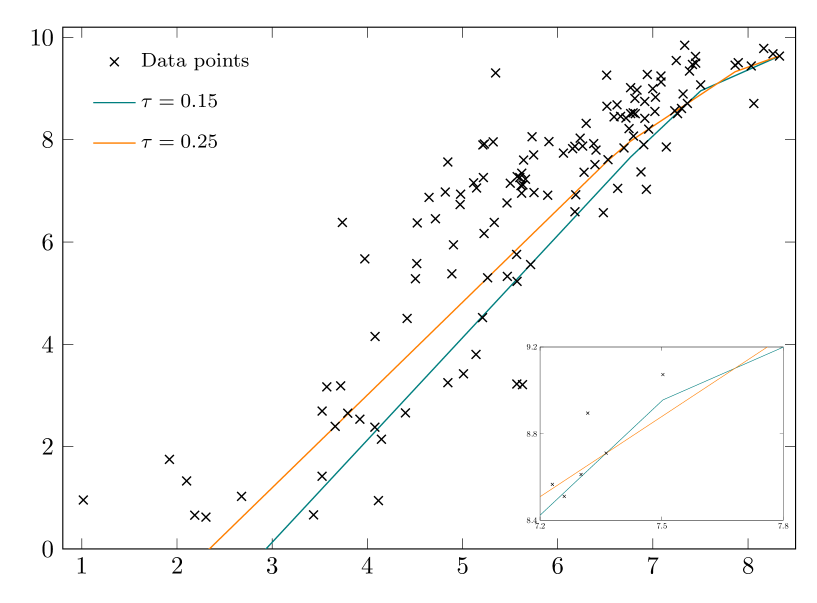
Figure A1: Illustration of the quantile crossing problem in CQR estimation.

Compared with the conventional full frontier estimation, the quantile function estimation is more robust to random noise, heteroscedasticity, and the choice of direction vectors. However, when separately estimating each conditional quantile function $Q_{y}(\tau\,|\,{\boldsymbol{x}})$, CQR is likely to violate the assumption that the distribution functions and their associated inverse functions should be monotone nondecreasing; see Fig. A1 for an example of the quantile crossing problem detected in our empirical application of CQR.

We notice that the quantile crossing problem could be addressed by simultaneous estimation, which imposes an extra set of linear non-crossing constraints in the CQR approach (see, e.g., Takeuchi2006, *Takeuchi2006; Wang2014c, *Wang2014c). Following Wang2014c, the simultaneous convex quantile regression (sCQR) estimator of $j$ conditional quantile functions at $0<\tau_{1}<\tau_{2}<\cdots<\tau_{j}<1$ is formulated as

$$\underset{\alpha,{\boldsymbol{\beta}},\varepsilon^{\text{+}},\varepsilon^{-},C}{\mathop{\min}} \,\sum\limits_{j=1}^{{\mathcal{J}}}\Big{(}\tau_{j}\sum\limits_{i=1}^{n}{\varepsilon_{i,j}^{+}}+(1-\tau_{j})\sum\limits_{i=1}^{n}{\varepsilon_{i,j}^{-}}\Big{)}$$ (4)

s.t. $$y_{i,j}=\mathbf{\alpha}_{i,j}+{\boldsymbol{\beta}}_{i,j}^{{}^{\prime}}{\boldsymbol{x}}_{i}+\varepsilon_{i,j}^{+}-\varepsilon_{i,j}^{-} \forall i,j$$

$$\alpha_{i,j}+{\boldsymbol{\beta}}_{i,j}^{{}^{\prime}}{\boldsymbol{x}}_{i}\leq\alpha_{h,j}+{\boldsymbol{\beta}}_{h,j}^{{}^{\prime}}{\boldsymbol{x}}_{i} \forall i,h,j$$

$$\alpha_{i,j}+{\boldsymbol{\beta}}_{i,j}^{{}^{\prime}}{\boldsymbol{x}}_{i}+C_{i,j}\leq\alpha_{i,j+1}+{\boldsymbol{\beta}}_{i,j+1}^{{}^{\prime}}{\boldsymbol{x}}_{i} \forall i,1\leq j\leq{\mathcal{J}}-1$$

$${\boldsymbol{\beta}}_{i,j}\geq{\boldsymbol{0}} \forall i,j$$

$$\varepsilon_{i,j}^{+}\geq 0,\ \varepsilon_{i,j}^{-}\geq 0 \forall i,j$$

where $C_{i,j}\geq 0$ are small nonnegative constants for quantiles, which are introduced in sCQR to ensure that $Q_{y}(\tau_{j}\,|\,{\boldsymbol{x}})\leq Q_{y}(\tau_{j+1}\,|\,{\boldsymbol{x}}),\forall i\text{ }\text{and}\text{ }j\in{\mathcal{J}}$. For the purpose of non-crossing, $C$ can simply be given by zero; that is, there may exist touching rather than crossing between two neighboring quantiles (see Fig. 1(a) for an illustration). In practice, however, after enforcing the non-crossing constraints, sCQR may violate the quantile property (Theorem 1) due to the fact that the approach simultaneously optimizes for both the quantile property and the non-crossing property (Takeuchi2006, *Takeuchi2006).

This paper proposes an alternative to sCQR to address the quantile crossing problem. By using the $L_{2}$-norm regularization on subgradients ${\boldsymbol{\beta}}_{i}$, we formulate penalized convex quantile regression (pCQR) as

$$\underset{\alpha,{\boldsymbol{\beta}},\varepsilon^{+},\varepsilon^{-}}{\mathop{\min}} \,\tau\sum\limits_{i=1}^{n}{\varepsilon_{i}^{+}}+(1-\tau)\sum\limits_{i=1}^{n}{\varepsilon_{i}^{-}}+\gamma\sum\limits_{i=1}^{n}||{\boldsymbol{\beta}}_{i}||^{2}_{2}$$ (5)

s.t. $$y_{i}=\alpha_{i}+{\boldsymbol{\beta}}_{i}^{{}^{\prime}}{\boldsymbol{x}}_{i}+\varepsilon_{i}^{+}-\varepsilon_{i}^{-} \forall i$$

$$\alpha_{i}+{\boldsymbol{\beta}}_{i}^{{}^{\prime}}{\boldsymbol{x}}_{i}\leq\alpha_{h}+{\boldsymbol{\beta}}_{h}^{{}^{\prime}}{\boldsymbol{x}}_{i} \forall i,h$$

$${\boldsymbol{\beta}}_{i}\geq{\boldsymbol{0}} \forall i$$

$$\varepsilon_{i}^{+}\geq 0,\ \varepsilon_{i}^{-}\geq 0 \forall i$$

where $\gamma\geq 0$ is the tuning parameter and $||\cdot||_{2}$ denotes the standard Euclidean norm. As $\gamma$ approaches to zero, pCQR (5) collapses to the original CQR problem (3). The rationale behind the avoidance of quantile crossing in pCQR lies in that as $\gamma\xrightarrow{}\infty$, the regularization will dominate the minimization and then all estimated subgradients ${\boldsymbol{\beta}}_{i}$ “flatten out” to 0. In this case, the estimated quantile functions will be horizontal lines (for $d=1$) or planes ($d>1$).

As $\gamma$ increases, the quantile property may also be disturbed in pCQR. But for sufficiently small $\gamma$, the quantile property can be guaranteed in theory. Therefore, we design the following Algorithm 1 to obtain the supremum $\gamma^{*}$ so as to avoid quantile crossing and ensure the quantile property as well as possible in estimating multiple quantile functions.

Data: $\{{\boldsymbol{x}}_{i},y_{i}\}_{i=1}^{n}\in{\mathbb{R}}^{d}\times{\mathbb{R}}$, $\tau_{1}$ and $\tau_{2}$ ($\tau_{1}<\tau_{2}$)

1 $\mathrm{out}=0$ and $\gamma=0$;

2 while $\mathrm{out}=0$ do

3       Solve problem (5) with quantiles $\tau_{1}$ and $\tau_{2}$, separately, to calculate $\hat{Q}_{y}(\tau_{1}\,|\,{\boldsymbol{x}}_{i})$ and $\hat{Q}_{y}(\tau_{2}\,|\,{\boldsymbol{x}}_{i})$;

4       if $\sum\limits_{i=1}^{n}\mathbf{1}_{\{\hat{Q}_{y}(\tau_{1}\,|\,{\boldsymbol{x}}_{i})-\hat{Q}_{y}(\tau_{2}\,|\,{\boldsymbol{x}}_{i})\leq 0\}}\neq n$ then

5             Re-solve problem (5) using the updated $\gamma$;

6            

7      else

8             $\mathrm{out}=1$;

9            

10      $\gamma=\gamma+0.01$;

11      

Result: $\gamma^{*}$

Algorithm 1 Searching the optimal tuning parameter $\gamma^{*}$.

We proceed to illustrate how non-crossing quantile functions look like with a real dataset used in Kuosmanen2020b. It contains plant-level data on 130 U.S. electric power plants operating in 2014; see Kuosmanen2020b for a more detailed description of the data. For the sake of demonstration, we simply consider a univariate case of one input and one output. The input is the total cost involved in electricity production and the output is the net electricity generation of each power plant. Both variables are in natural logarithm.

An application of CQR to the empirical data finds that the 15${}^{\text{th}}$ quantile curve crosses the 25${}^{\text{th}}$ quantile curve twice (see Fig. A1). We then demonstrate how the sCQR and pCQR approaches can address this problem. It is evident from Fig. 1 that both approaches manage to circumvent the quantile crossing problem; that is, we observe that $\widehat{Q}_{y}(0.25\,|\,{\boldsymbol{x}}_{i})$ is greater than or equal to $\widehat{Q}_{y}(0.15\,|\,{\boldsymbol{x}}_{i})$ in both approaches. However, the shapes of the estimated quantile functions in Figs. 1(a) and 1(b) (see particularly the upper right corner) are slightly different. As mentioned earlier, this difference arises because sCQR tries to simultaneously optimize for the non-crossing property, the quantile property, and the production axioms, whereas the pCQR approach independently estimates the quantile production functions. Further, the difference affects which approach can better retain the quantile property.

3 Monte Carlo study

We perform a Monte Carlo study to examine whether pCQR or sCQR can better satisfy the quantile property while addressing quantile crossing. Consider the following data generating process (Dai2021a, *Dai2021a)

$$y_{i}=\prod\limits_{d=1}^{D}{\boldsymbol{x}}^{\frac{0.8}{d}}_{d,i}+v_{i}-u_{i},$$

where the input matrix ${\boldsymbol{x}}_{i}\in{\mathbb{R}}^{n\times d}$ is generated independently from $U[1,10]$, and noise $v_{i}$ and inefficiency $u_{i}$ are drawn independently from $N(0,\sigma_{v}^{2})$ and $N^{+}(0,\sigma_{u}^{2})$, respectively. To investigate the robustness of the quantile approaches, following Aigner1977 we use different combinations of noise ($\sigma$) and signal to noise ratio ($\lambda$), that is, ($\sigma^{2}$, $\lambda$) = (1.88, 1.66), (1.63, 1.24), and (1.35, 0.83).

We consider 54 scenarios with $n\in\{99,199,499\}$, $d\in\{2,3,4\}$, and $\tau\in\{0.85,0.90,0.95\}$. Each scenario is replicated 500 times using the pyStoNED package (Dai2021b, *Dai2021b) on Python with the standard solver Mosek (9.3). We then compute the ramp loss ($\text{RL}=|\frac{1}{n}\sum_{i=1}^{n}\textbf{1}_{y_{i}>{{\widehat{Q}}_{y}}(\tau\,|\,{\boldsymbol{x}}_{i})}-\tau|$) (Takeuchi2006, *Takeuchi2006) to examine the quantile property and the mean squared error (MSE) to evaluate the finite-sample performance. Replications for which no quantile crossing happen (i.e., $\gamma^{*}=0$) are excluded from the calculations of RL and MSE. Note that the smaller the ramp loss, the better the quantile performance.

Tables 1 and A1 present the estimated ramp loss and MSE statistics across different scenarios. The results clearly show that compared with sCQR, pCQR has lower ramp loss in virtually all the scenarios and lower MSE in all the scenarios. This is because the optimal tuning parameter $\gamma^{*}$ used in the pCQR simulations mainly locates in the interval $[0.01,0.03]$ (see Fig. 2), suggesting that the quantile property can be guaranteed to a certain extent and thus pCQR can better fit the true quantile functions. Several other findings are summarized as follows:

• The higher the dimension or the noise in data space, the lower the ramp loss. As $d$ or $\sigma$ increases, the data space becomes more sparse, thereby indicating that the probability of crossing between two neighboring quantiles is relatively small.

• The differences in the ramp loss among quantiles in pCQR are smaller than those in sCQR due to the different estimation strategies, i.e., independent and simultaneous estimation, respectively.

• For both approaches, the MSE increases as more inputs are included and decreases as the sample size gets larger.

• The performance of both approaches in terms of MSE becomes worse as the signal to noise ratio increases.

Overall, the pCQR approach can better satisfy the quantile property and fit the true quantile functions while at the same time addressing the quantile crossing problem. Regularizing the quantile function, instead of imposing an extra set of non-crossing constraints, proves a better remedy to quantile crossing according to our simulations.

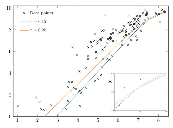
(a) sCQR ($C=0$)

(b) pCQR ($\gamma^{*}=0.01$)

Figure 1: Empirical illustration of estimated non-crossing quantile functions using the U.S. power plant data.

Table 1: Ramp loss and MSE of two neighboring quantiles with $n=499$.

$d$	($\sigma^{2},\lambda$)	$\tau_{1}$	$\tau_{2}$	RL${}_{\tau_{1}}$		MSE${}_{\tau_{1}}$		RL${}_{\tau_{2}}$		MSE${}_{\tau_{2}}$
				pCQR	sCQR	pCQR	sCQR	pCQR	sCQR	pCQR	sCQR
2	(1.35, 0.83)	0.85	0.90	0.928	0.993	0.065	0.093	0.968	1.035	0.075	0.115
		0.90	0.95	0.998	1.078	0.074	0.117	1.035	1.108	0.095	0.176
	(1.63, 1.24)	0.85	0.90	0.899	0.953	0.075	0.108	0.933	1.028	0.085	0.135
		0.90	0.95	0.972	1.061	0.081	0.134	0.991	1.051	0.108	0.208
	(1.88, 1.66)	0.85	0.90	0.898	0.967	0.079	0.117	0.984	1.069	0.095	0.155
		0.90	0.95	0.890	0.963	0.093	0.153	0.923	1.012	0.117	0.228
3	(1.35, 0.83)	0.85	0.90	0.811	0.942	0.103	0.205	0.826	0.947	0.115	0.265
		0.90	0.95	0.775	0.902	0.122	0.253	0.745	0.860	0.166	0.402
	(1.63, 1.24)	0.85	0.90	0.832	0.950	0.110	0.226	0.832	0.940	0.127	0.296
		0.90	0.95	0.827	0.959	0.138	0.281	0.751	0.878	0.175	0.435
	(1.88, 1.66)	0.85	0.90	0.792	0.913	0.127	0.250	0.827	0.960	0.144	0.325
		0.90	0.95	0.789	0.914	0.172	0.332	0.749	0.899	0.214	0.512
4	(1.35, 0.83)	0.85	0.90	0.658	0.837	0.163	0.368	0.671	0.833	0.187	0.484
		0.90	0.95	0.627	0.794	0.207	0.487	0.481	0.601	0.269	0.750
	(1.63, 1.24)	0.85	0.90	0.587	0.801	0.168	0.397	0.627	0.795	0.193	0.526
		0.90	0.95	0.696	0.861	0.217	0.535	0.539	0.700	0.279	0.828
	(1.88, 1.66)	0.85	0.90	0.584	0.793	0.189	0.446	0.622	0.793	0.218	0.589
		0.90	0.95	0.646	0.795	0.285	0.581	0.504	0.640	0.381	0.920

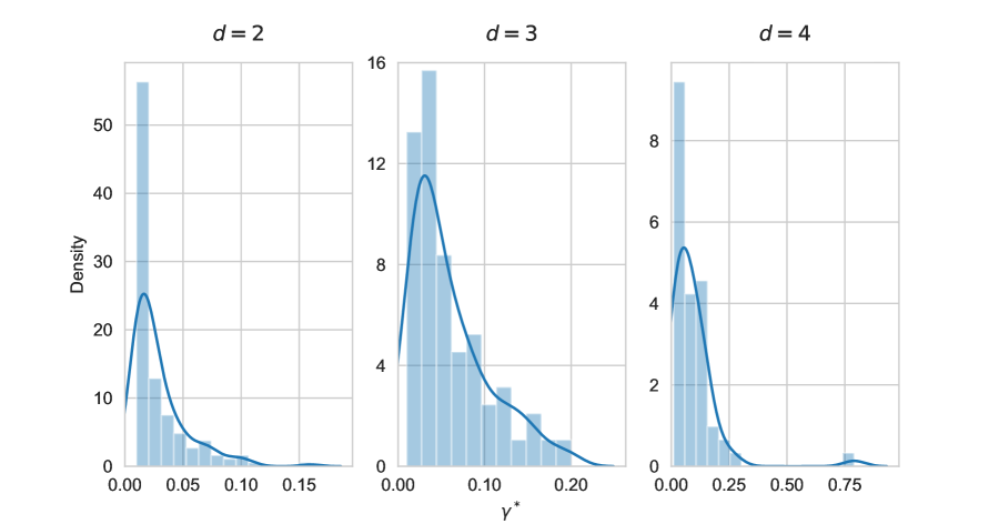
Figure 2: Empirical distribution of $\gamma^{*}$ with $n=499$, $(\sigma^{2},\lambda)=(1.35,0.83)$, $\tau_{1}=0.85$, and $\tau_{2}=0.90$.

4 Conclusions

In this paper, a penalized convex quantile regression approach has been developed to address the quantile crossing problem. The proposed algorithm can search the optimal tuning parameter such that the occurrences of quantile crossing are avoided and the quantile property is ensured as well as possible. A Monte Carlo study confirms the superiority of the proposed approach compared to previous work in addressing the quantile crossing problem. We believe the proposed approach can be readily extended from convex quantile regression to other nonparametric and parametric quantile regression techniques. We leave such extensions as fascinating avenues for future research.

Appendix

A Supplementary tables and figures

Table A1: Ramp loss and MSE of two neighboring quantiles with $n=99$ and $199$.

$n$	$d$	($\sigma^{2},\lambda$)	$\tau_{1}$	$\tau_{2}$	RL${}_{\tau_{1}}$		MSE${}_{\tau_{1}}$		RL${}_{\tau_{2}}$		MSE${}_{\tau_{2}}$
					pCQR	sCQR	pCQR	sCQR	pCQR	sCQR	pCQR	sCQR
99	2	(1.35, 0.83)	0.85	0.90	0.824	0.882	0.239	0.350	0.869	0.884	0.276	0.444
			0.90	0.95	0.849	0.899	0.300	0.459	0.835	0.794	0.396	0.683
		(1.63, 1.24)	0.85	0.90	0.806	0.882	0.248	0.378	0.857	0.904	0.287	0.484
			0.90	0.95	0.888	0.935	0.324	0.481	0.867	0.845	0.427	0.727
		(1.88, 1.66)	0.85	0.90	0.831	0.898	0.272	0.435	0.891	0.916	0.327	0.556
			0.90	0.95	0.857	0.918	0.336	0.534	0.792	0.809	0.439	0.803
	3	(1.35, 0.83)	0.85	0.90	0.719	0.753	0.349	0.619	0.667	0.702	0.400	0.777
			0.90	0.95	0.626	0.687	0.442	0.807	0.446	0.381	0.618	1.262
		(1.63, 1.24)	0.85	0.90	0.671	0.721	0.400	0.688	0.632	0.657	0.469	0.878
			0.90	0.95	0.629	0.695	0.516	0.875	0.393	0.364	0.713	1.392
		(1.88, 1.66)	0.85	0.90	0.677	0.741	0.439	0.782	0.622	0.676	0.500	0.989
			0.90	0.95	0.611	0.662	0.541	1.046	0.437	0.404	0.742	1.651
	4	(1.35, 0.83)	0.85	0.90	0.412	0.491	0.591	1.041	0.334	0.342	0.715	1.384
			0.90	0.95	0.382	0.421	0.798	1.381	0.239	0.194	1.118	2.148
		(1.63, 1.24)	0.85	0.90	0.455	0.550	0.688	1.139	0.403	0.427	0.833	1.497
			0.90	0.95	0.381	0.395	0.874	1.491	0.229	0.182	1.264	2.384
		(1.88, 1.66)	0.85	0.90	0.502	0.606	0.664	1.180	0.450	0.468	0.813	1.567
			0.90	0.95	0.412	0.449	0.931	1.624	0.239	0.231	1.339	2.567
199	2	(1.35, 0.83)	0.85	0.90	0.837	0.916	0.139	0.201	0.914	0.964	0.160	0.251
			0.90	0.95	0.914	0.997	0.159	0.250	0.934	0.981	0.206	0.372
		(1.63, 1.24)	0.85	0.90	0.869	0.957	0.140	0.210	0.935	0.978	0.166	0.276
			0.90	0.95	0.944	1.016	0.178	0.291	0.959	1.003	0.233	0.427
		(1.88, 1.66)	0.85	0.90	0.868	0.931	0.150	0.236	0.894	0.949	0.186	0.311
			0.90	0.95	0.945	1.012	0.186	0.322	0.948	0.968	0.223	0.459
	3	(1.35, 0.83)	0.85	0.90	0.656	0.777	0.203	0.374	0.703	0.779	0.231	0.485
			0.90	0.95	0.733	0.830	0.256	0.472	0.561	0.621	0.338	0.721
		(1.63, 1.24)	0.85	0.90	0.696	0.815	0.221	0.436	0.708	0.790	0.248	0.568
			0.90	0.95	0.748	0.881	0.266	0.550	0.631	0.707	0.364	0.848
		(1.88, 1.66)	0.85	0.90	0.713	0.837	0.249	0.461	0.740	0.839	0.277	0.595
			0.90	0.95	0.657	0.716	0.335	0.653	0.516	0.553	0.438	1.013
	4	(1.35, 0.83)	0.85	0.90	0.584	0.703	0.282	0.663	0.568	0.597	0.328	0.876
			0.90	0.95	0.452	0.570	0.409	0.918	0.350	0.364	0.537	1.430
		(1.63, 1.24)	0.85	0.90	0.503	0.670	0.331	0.736	0.507	0.605	0.380	0.969
			0.90	0.95	0.453	0.569	0.476	0.974	0.321	0.354	0.617	1.533
		(1.88, 1.66)	0.85	0.90	0.428	0.622	0.354	0.806	0.427	0.554	0.423	1.074
			0.90	0.95	0.472	0.630	0.515	1.084	0.332	0.375	0.657	1.687

References

- [1] \harvarditem[Aigner et al.]Aigner, Lovell \harvardand Schmidt1977Aigner1977 Aigner, D., Lovell, C. A. K. \harvardand Schmidt, P. \harvardyearleft1977\harvardyearright, Formulation and estimation of stochastic frontier production function models, Journal of Econometrics 6, 21–37.
- [2] \harvarditem[Bondell et al.]Bondell, Reich \harvardand Wang2010Bondell2010 Bondell, H. D., Reich, B. J. \harvardand Wang, H. \harvardyearleft2010\harvardyearright, Noncrossing quantile regression curve estimation, Biometrika 97, 825–838.
- [3] \harvarditem[Chernozhukov et al.]Chernozhukov, FernÁndez-Val \harvardand Galichon2010Chernozhukov2010 Chernozhukov, V., FernÁndez-Val, I. \harvardand Galichon, A. \harvardyearleft2010\harvardyearright, Quantile and probability curves without crossing, Econometrica 78, 1093–1125.
- [4] \harvarditemDai2021Dai2021a Dai, S. \harvardyearleft2021\harvardyearright, Variable selection in convex quantile regression: L1-norm or L0-norm regularization?, arxiv preprint arxiv:2107.03119.
- [5] \harvarditem[Dai et al.]Dai, Fang, Lee \harvardand Kuosmanen2021Dai2021b Dai, S., Fang, Y. H., Lee, C. Y. \harvardand Kuosmanen, T. \harvardyearleft2021\harvardyearright, pyStoNED: A Python package for convex regression and frontier estimation, arxiv preprint arxiv:2109.12962.
- [6] \harvarditemDette \harvardand Volgushev2008Dette2008 Dette, H. \harvardand Volgushev, S. \harvardyearleft2008\harvardyearright, Non-crossing non-parametric estimates of quantile curves, Journal of the Royal Statistical Society. Series B (Statistical Methodology) 70, 609–627.
- [7] \harvarditemHe1997He1997 He, X. \harvardyearleft1997\harvardyearright, Quantile curves without crossing, American Statistician 51, 186–192.
- [8] \harvarditem[Jradi et al.]Jradi, Parmeter \harvardand Ruggiero2019Jradi2019 Jradi, S., Parmeter, C. F. \harvardand Ruggiero, J. \harvardyearleft2019\harvardyearright, Quantile estimation of the stochastic frontier model, Economics Letters 182, 15–18.
- [9] \harvarditemKuosmanen \harvardand Zhou2021Kuosmanen2020b Kuosmanen, T. \harvardand Zhou, X. \harvardyearleft2021\harvardyearright, Shadow prices and marginal abatement costs: Convex quantile regression approach, European Journal of Operational Research 289, 666–675.
- [10] \harvarditemLiu \harvardand Wu2009Wu2009a Liu, Y. \harvardand Wu, Y. \harvardyearleft2009\harvardyearright, Stepwise multiple quantile regression estimation using non-crossing constraints, Statistics and Its Interface 2, 299–310.
- [11] \harvarditem[Takeuchi et al.]Takeuchi, Le, Sears \harvardand Smola2006Takeuchi2006 Takeuchi, I., Le, Q. V., Sears, T. D. \harvardand Smola, A. J. \harvardyearleft2006\harvardyearright, Nonparametric quantile estimation, Journal of Machine Learning Research 7, 1231–1264.
- [12] \harvarditem[Tsionas et al.]Tsionas, Assaf \harvardand Andrikopoulos2020Tsionas2020b Tsionas, M. G., Assaf, A. G. \harvardand Andrikopoulos, A. \harvardyearleft2020\harvardyearright, Quantile stochastic frontier models with endogeneity, Economics Letters 188.
- [13] \harvarditem[Wang et al.]Wang, Wang, Dang \harvardand Ge2014Wang2014c Wang, Y., Wang, S., Dang, C. \harvardand Ge, W. \harvardyearleft2014\harvardyearright, Nonparametric quantile frontier estimation under shape restriction, European Journal of Operational Research 232, 671–678.
- [14] \harvarditemZhao2021Zhao2021 Zhao, S. \harvardyearleft2021\harvardyearright, Quantile estimation of stochastic frontier models with the normal-half normal specification: A cumulative distribution function approach, Economics Letters 206, 109998.
- [15]