Training Fully Connected Neural Networks is $\exists\mathbb{R}$-Complete

Abstract

We consider the algorithmic problem of finding the optimal weights and biases for a two-layer fully connected neural network to fit a given set of data points. This problem is known as empirical risk minimization in the machine learning community. We show that the problem is $\exists\mathbb{R}$-complete. This complexity class can be defined as the set of algorithmic problems that are polynomial-time equivalent to finding real roots of a polynomial with integer coefficients. Furthermore, we show that arbitrary algebraic numbers are required as weights to be able to train some instances to optimality, even if all data points are rational. Our results hold even if the following restrictions are all added simultaneously:

• There are exactly two output neurons.

• There are exactly two input neurons.

• The data has only $13$ different labels.

• The number of hidden neurons is a constant fraction of the number of data points.

• The target training error is zero.

• The $\mathrm{ReLU}$ activation function is used.

This shows that even very simple networks are difficult to train. The result explains why typical methods for -complete problems, like mixed-integer programming or SAT-solving, cannot train neural networks to global optimality, unless $\NP=\exists\mathbb{R}$. We strengthen a recent result by Abrahamsen, Kleist and Miltzow [NeurIPS 2021].

Acknowledgments. Christoph Hertrich is supported by the European Research Council (ERC) under the European Union’s Horizon 2020 research and innovation programme (grant agreement ScaleOpt–757481). Tillmann Miltzow is generously supported by the Netherlands Organisation for Scientific Research (NWO) under project no. 016.Veni.192.250. Simon Weber is supported by the Swiss National Science Foundation under project no. 204320.

1 Introduction

The usage of neural networks in modern computer science is ubiquitous. It is arguably the most powerful tool at our hands in machine learning [GBC16]. One of the most fundamental algorithmic questions asks for the algorithmic complexity to actually train a neural network. For arbitrary network architectures, Abrahamsen, Kleist and Miltzow [AKM21] showed that the problem is $\exists\mathbb{R}$-complete already for two-layer neural networks and linear activation functions. The complexity class $\exists\mathbb{R}$ is defined as the family of algorithmic problems that are polynomial-time equivalent to finding real roots of polynomials with integer coefficients. See Section 1.3 for a proper introduction. Under the commonly believed assumption that $\exists\mathbb{R}$ is a strict superset of , this implies that training a neural network is harder than -complete problems.

The result by Abrahamsen, Kleist and Miltzow [AKM21] has one major downside, namely that the network architecture is adversarial: The hardness inherently relies on choosing a network architecture that is particularly difficult to train. The instances by Abrahamsen, Kleist and Miltzow could be trivially trained with fully connected neural networks, as they reduce to matrix factorization. This stems from the fact that they use the identity function as the activation function. While intricate network architectures (for example, convolutional and residual neural networks, pooling, autoencoders, generative adversarial neural networks) are common in practice, they are usually designed in a way that facilitates training rather than making it difficult [GBC16]. Here, we strengthen the result in [AKM21] by showing hardness for fully connected two-layer neural networks. This shows that $\exists\mathbb{R}$-hardness does not stem from one specifically chosen worst-case architecture but is inherent in the neural network training problem itself. Although in practice a host of different architectures are used, fully connected two-layer neural networks are arguably the most basic ones and they are often part of more complicated network architectures [GBC16]. We can show hardness even for the most basic case of fully connected two-layer $\mathrm{ReLU}$ neural networks with exactly two input and output dimensions.

In the following, we give different perspectives on how to interpret our findings. Then, we present precise definitions and state our results formally. This is the basis for an in-depth discussion of the strengths and limitations from different perspectives. Thereafter we give an introduction to related work on $\exists\mathbb{R}$-completeness and theory on neural networks. We finish the introduction by giving the key ingredients of the proof of our result.

Implications of $\exists\mathbb{R}$-Completeness.

Even though the class $\exists\mathbb{R}$ is defined via the existence of real roots of polynomials, it is a class in the standard word RAM (equivalently, Turing machine) model, just like ¶, , and . This is possible because the input polynomials are encoded via integers using the standard bit-encoding. Therefore, the word RAM is the default model in the whole paper and we explicitly point out when we use statements involving other machine models. It is known that $\NP\subseteq\exists\mathbb{R}\subseteq\PSPACE$, and it is widely believed that both inclusions are strict. Therefore, proving $\exists\mathbb{R}$-completeness of a problem that is already known to be -hard is a valuable contribution for at least two reasons: Firstly, from a theoretical standpoint we are always interested in the exact complexity of an algorithmic problem. Secondly, $\exists\mathbb{R}$-completeness provides a better understanding of the difficulties that need to be overcome when designing algorithms for the considered problem: While there is a wide collection of extremely optimized off-the-shelf tools like SAT- or mixed-integer programming solvers applicable to many -complete problems, no such general purpose tools are available for $\exists\mathbb{R}$-complete problems. In fact, using these tools is most likely not sufficient to solve $\exists\mathbb{R}$-complete problems, because this would imply $\NP=\exists\mathbb{R}$.

As an illustrative example of how difficult it is to solve $\exists\mathbb{R}$-complete problems, consider the problem of packing unit-squares into a square container [AMS20]: Figure 1 shows how to optimally pack five unit-squares into a minimum square container and the best known (but potentially not optimal) way to pack eleven unit-squares.

Figure 1: Left: Packing of five unit squares into a minimum square container. Right: The best known packing of eleven unit squares into a square container [GR05]. This is not known to be optimal.

One method that can sometimes be used to get “good” solutions (but without any approximation guarantees) for $\exists\mathbb{R}$-complete problems is gradient descent, for example for graph drawing [ADLD⁺20]. Note that this also applies in the context of training neural networks, where a bunch of different gradient descent variants powered by backpropagation are widely used. However, when using gradient descent we usually do not get any guarantees on the quality of the obtained solutions or on the time it takes to compute them [DJL⁺17]. Thus it would be very desirable to use other methods, like SAT- or mixed-integer programming solvers that are reliable and widely used in practice for many -complete problems. $\exists\mathbb{R}$-completeness indicates that these methods cannot succeed unless $\NP=\exists\mathbb{R}$.

Let us stress that $\exists\mathbb{R}$-completeness does not rule out any hope for good heuristics. Other $\exists\mathbb{R}$-complete problems like the art gallery problem can be solved in practice via custom heuristics, sometimes also in combination with integer programming solvers [dRdSF⁺16]. Under additional assumptions, those methods are even shown to work reliably [HM21]. Thus, $\exists\mathbb{R}$-completeness of training neural networks does not exclude the possibility of appropriate assumptions that make training tractable. Assumptions are appropriate if they are mathematically natural and related to practice. For instance, if there is only one output neuron, training two-layer $\mathrm{ReLU}$ neural networks to global optimality is contained in  [ABMM18].

Relation to Previous Results.

It is well-known that minimizing the training error of a neural network is a computationally hard problem for a large variety of activation functions and architectures [SSBD14]. For $\mathrm{ReLU}$ networks, -hardness, parameterized hardness, and inapproximability results have been established even for the simplest possible architecture consisting of only a single $\mathrm{ReLU}$ neuron [BDL22, DWX20, FHN22, GKMR21]. On the positive side, the seminal algorithm by Arora, Basu, Mianjy, and Mukherjee [ABMM18] solves empirical risk minimization for 2-layer $\mathrm{ReLU}$ networks and one-dimensional output to global optimality. It was later extended to a more general class of loss functions by Froese, Hertrich, and Niedermeier [FHN22]. The running time is exponential in the number of neurons in the hidden layer and in the input dimension, but polynomial in the number of data points if the former two parameters are considered to be a constant. In particular, this algorithm implies that the problem is contained in . The idea is to perform a combinatorial search over all possible activation patterns (whether the input to each $\mathrm{ReLU}$ is positive or negative). Since then, it has been an open question whether an exact algorithm of this type can be found for more complex architectures as well. Our result now yields an explanation why no such algorithm has been found: adding only a second output neuron to the architecture considered by Arora, Basu, Mianjy, and Mukherjee [ABMM18] makes empirical risk minimization $\exists\mathbb{R}$-hard, implying that a combinatorial search algorithm of that flavor cannot exist unless $\NP{}=\exists\mathbb{R}{}$.

Relation to Learning Theory.

In this paper we purely focus on the computational complexity of empirical risk minimization, that is, minimizing the training error. In the machine learning practice, one usually desires to achieve low generalization error, which means to use the training data to achieve good predictions on unseen test samples.

To formalize the concept of the generalization error, one needs to combine the computational aspect with a statistical one. There are various models to do so in the literature, the most famous one being probably approximately correct (PAC) learnability [SSBD14, Val84]. While empirical risk minimization and learnability are two different questions, they are strongly intertwined. We will provide more details about these interconnections when we discuss further related literature.

Despite the close connections between empirical risk minimization and learnability, to the best of our knowledge, the $\exists\mathbb{R}$-hardness of the former has no direct implications on the complexity of the latter. Still, since empirical risk minimization is the most common learning paradigm in practice, our work is arguably also interesting in the context of learning theory.

1.1 Definitions and Results.

In order to describe our results, we need to introduce the standard definitions concerned with the type of neural networks studied by us.

Definition 1 (Neural Network).

A neural network is a directed acyclic graph $N=(V,E)$ (the architecture or network) with edge weights $w_{uv}\in\mathbb{R}$ for each $uv\in E$. The vertices of $N$ are called neurons. The neurons $S\subseteq V$ with in-degree zero are called inputs, similarly the neurons $T\subseteq V$ with out-degree zero are called outputs. All other neurons are hidden neurons. Additionally there is a bias $b_{v}\in\mathbb{R}$ and an activation function $\varphi_{v}$ for each hidden neuron $v\in V\setminus(S\cup T)$.

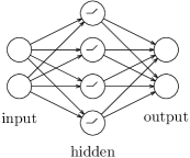
Figure 2: A neural network is defined as a directed acyclic graph. Sources and sinks are called input and output neurons. The symbol inside the hidden neurons expresses the $\mathrm{ReLU}$ activation function. The pictured neural network is a fully connected two-layer neural network.

The vertices can be partitioned into layers $V=V_{0}\cup\ldots\cup V_{k+1}$ where $S=V_{0}$ and $T=V_{k+1}$, such that each edge goes from $V_{i}$ to $V_{i+1}$. The layers $V_{1},\ldots,V_{k}$ are called hidden layers. The neural network is fully connected if it contains exactly all possible edges between two consecutive layers. The probably most commonly used activation function [ABMM18, GBB11, GBC16] is the rectified linear unit (ReLU) defined as $\mathrm{ReLU}:\mathbb{R}\to\mathbb{R}$, $x\mapsto\max\{0,x\}$.

In case that there is only one hidden layer, we speak (confusingly) of a two-layer neural network. The name stems from the interpretation that there are two layers of edges, even though the vertex set is split into three layers. See Figure 2 for a small fully connected two-layer $\mathrm{ReLU}$ neural network.

Given a neural network architecture $N$ as defined above, assume that we fixed an ordering on $S$ and $T$. Then $N$ realizes a function $f(\cdot,\Theta):\mathbb{R}^{|S|}\to\mathbb{R}^{|T|}$, where $\Theta$ denotes the weights and biases that parameterize the function. For $x\in\mathbb{R}^{|S|}$ we define $f(\cdot,\Theta)$ inductively: The $i$-th input neuron forwards the $i$-th component of $x$ to all its outgoing neighbors. Each hidden neuron forms the weighted sum over all incoming values, adds its bias, applies the activation function to this sum and forwards it to all outgoing neighbors. An output neuron again forms the weighted sum over all incoming values but does not add a bias and does not apply any activation function.

Note that it is possible to also use an activation function at the output neurons. Here we restrict ourselves to the case that activation functions are only used at hidden neurons, as we do not want to confuse the reader by considering too many variants of two-layer neural networks. Architectures with activation functions at the output neurons seem to be less commonly used in practice [GBC16], but we believe that our proofs could also be adapted to this case.

We introduced neural networks using the language of graphs. We want to point out that this is only one possible perspective. Fully connected neural networks can also be described as the alternating composition of affine/linear functions and the (componentwise) activation function.

Definition 2 (Train-F2NN).

We define the problem of training a fully connected two-layer neural network (Train-F2NN) to be the following decision problem:

Input: A $5$-tuple $(m,\varphi,D,\gamma,c)$ where

• $m\in\mathbb{N}$ encoded in unary is the size of the hidden layer,

• $\varphi:\mathbb{R}\to\mathbb{R}$ is an activation function to be used at all neurons in the hidden layer,

• $D$ is a set of $n$ data points of the form $(x;y)\in\mathbb{Q}^{|S|}\times\mathbb{Q}^{|T|}$,

• $\gamma\in\mathbb{Q}_{\geq 0}$ is the target error, and

• $c:\mathbb{R}^{|T|}\times\mathbb{R}^{|T|}\to\mathbb{R}_{\geq 0}$ is the loss function.

Question: Are there weights and biases $\Theta$ such that $\sum_{(x;y)\in D}c(f(x,\Theta),y)\leq\gamma$?

The reason to encode $m$ in unary is to guarantee that the described neural network has size polynomial in the input size. Furthermore, we assume that the loss function is honest, meaning that it returns zero if and only if the data is fit exactly. We will see that this is the only required assumption on the loss function to prove $\exists\mathbb{R}$-hardness of the zero-error case ($\gamma=0)$.

To prove $\exists\mathbb{R}$-membership, we further assume that the loss function can be computed in polynomial time on the real RAM. The real RAM is a model of computation similar to the well-known word RAM that has additional registers to store real numbers with infinite precision. Addition, subtraction, multiplication, division and even taking square roots of real numbers are supported in constant time. As $\exists\mathbb{R}$-membership has already been shown in [AKM21], we omit a formal discussion of the real RAM here and point the interested reader to [EvdHM20].

We are now ready to state our main result:

Theorem 3.

The problem Train-F2NN is $\exists\mathbb{R}$-complete, even if:

• There are exactly two input neurons.

• There are exactly two output neurons.

• The number of hidden neurons is a constant fraction of the number of data points.

• The data has only $13$ different labels.

• The target error is $\gamma=0$.

• The $\mathrm{ReLU}$ activation function is used.

Apart from settling the precise computational complexity status of the problem to train fully-connected neural networks, our result implies that any approach to solve Train-F2NN to global optimality must involve more sophisticated methods than those used for typical -complete problems.

Corollary 4.

Unless $\NP=\exists\mathbb{R}$, there does not exist an algorithm for Train-F2NN, which runs in polynomial time and has access to an oracle for an -complete problem.

Proof.

Every such algorithm would imply $\NP$-membership of the $\exists\mathbb{R}$-complete problem Train-F2NN by using the outputs of the oracle calls as an -certificate. ∎

Additionally, we show that our reduction to prove $\exists\mathbb{R}$-hardness also implies the following algebraic universality statement:

Theorem 5.

Let $\alpha$ be an algebraic number. Then there exists an instance of Train-F2NN, which has a solution when the weights and biases $\Theta$ are restricted to $\mathbb{Q}[\alpha]$, but no solution when the weights and biases $\Theta$ are restricted to a field $\mathbb{F}$ not containing $\alpha$.

Algebraic universality is known to hold for various $\exists\mathbb{R}$-complete problems [AM19]. On the other hand, this is not an automatism: Algebraic universality cannot occur in problems where the solution space is open, which is the case in some problems of recognizing certain intersection graphs [CFM⁺18, KM94].

1.2 Discussion

In this section, we discuss our results from various perspectives, pointing out strengths and limitations. This includes, but is not limited to, identifying angles from which it is tight and angles from which it leaves room for further research.

Input Neurons.

In practice, neural networks are often trained on high dimensional data, thus having only two input neurons is even more restrictive than the practical setting. Note that we easily obtain hardness for higher input dimensions by simply placing all data points of our reduction into a two-dimensional subspace. The precise complexity of training fully connected two-layer neural networks with only one-dimensional input and multi-dimensional output remains unknown. While this setting does not have practical relevance, we are still curious about this open question from a purely mathematical perspective.

Output Neurons.

If there is only one output neuron instead of two, then the problem is known to be contained in  [ABMM18]. See also the discussion about the related work above. Thus, unless $\NP=\exists\mathbb{R}$, our result cannot be improved further in terms of the number of output neurons.

Hidden Neurons.

Consider the situation that the number $m$ of hidden neurons is larger than the number $n$ of data points. If there are no two contradicting data points with $x_{i}=x_{j}$ but $y_{i}\neq y_{j}$, then it is known that we can always fit all the data points [ZBH⁺21]. Thus, having a linear number of data points in terms of $m$ is the fewest possible we can expect. We wonder whether it is possible to show $\exists\mathbb{R}$-completeness with $n\leq(1+\varepsilon)m$ for every fixed $\varepsilon$.

Output Labels.

The number of labels, that is, different values for $y\in\mathbb{Q}^{|T|}$ in the data set $D$, used in our reduction is the small constant $13$. A small set of possible labels shows relevance of our results to practice, where we are often confronted with a large number of data points but a much smaller number of labels, for instance, in classification tasks. The set of labels used by us is

$$\{(-2,6),(-1,-1),(-1,0),(0,-1),(0,0),(0,3),(2,2),(3,3),(3,6),(4,4),(6,-2),(6,6),(10,10)\}\text{.}$$

If all labels are contained in a one-dimensional affine subspace the problem is in , as then they can be projected down to one-dimensional labels and the problem can be solved with the algorithm by Arora, Basu, Mianjy, and Mukherjee [ABMM18]. As any two labels span a one-dimensional affine subspace, the problem can only be $\exists\mathbb{R}$-hard if at least three different affinely independent output labels are present.

We are not particularly interested in closing the gap between $13$ and $3$ output labels, but it would be interesting to investigate the complexity of the problem when output labels have more structure. For example, in classification tasks one often uses one-hot encodings, where for $k$ classes, a $k$-dimensional output space is used and all labels have the form $(0,\ldots,0,1,0,\ldots,0)$. Note that in this case, at least three output dimensions are needed to obtain three different labels.

Target Error.

We show hardness for the case with target error $\gamma=0$. Arguably, it is often not required in practice to fit the data exactly. It is not too difficult to see that we can easily modify the value of $\gamma$ by adding inconsistent data points that can only be fit best in exactly one way. The precise choice of these inconsistent data points heavily depends on the loss function. In conclusion, for different values of $\gamma$, the decision problem does not get easier.

Activation Functions.

Let us point out that the $\mathrm{ReLU}$ activation function is currently still the most commonly used activation function in practice [ABMM18, GBB11, GBC16]. Our methods are probably easily adaptable to other piecewise linear activation functions, for example, leaky ReLUs. Having said that, our methods are not applicable to other types of activation functions at all, for example, Sigmoid, soft $\mathrm{ReLU}$ or step functions. We want to point out that Train-F2NN (and even training of arbitrary other architectures) is in  in case a step function is used as the activation function [KB22]. For the Sigmoid and soft $\mathrm{ReLU}$ function it is not even clear whether the problem is decidable, as trigonometric functions and exponential functions are not computable even on the real RAM [EvdHM20, Ric69].

Lipschitz Continuity and Regularization.

The set of data points created in the proof of Theorem 3 is intuitively very tame. To make this more precise, our reduction fulfills the following property: There is a bounded Lipschitz constant $L$, which does not depend on the specific problem instance ($L=25$ safely works for our reduction and $L$ could be made arbitarily small by downscaling all data points), such that either there exists $\Theta$ such that the function $f(\cdot,\Theta)$ is Lipschitz continuous with Lipschitz constant $L$ and fits the data points, or there is no $\Theta$ at all to fit the data points. Note that Lipschitz continuity is also related to overfitting and regularization [GFPC21]. Recall that the purpose of regularization is to prefer simpler functions over more complicated ones. Being Lipschitz continuous with a small Lipschitz constant essentially means that the function is pretty flat. It is particularly remarkable that we can show hardness even for small Lipschitz constants since Lipschitz continuity has been a crucial assumption in several recent results about training and learning ReLU networks, for example, [BMP18, CKM22, GKKT17].

Other Architectures.

While we consider fully connected two-layer networks as the most important case, we are also interested in $\exists\mathbb{R}$-hardness results for other network architectures. Specifically, fully connected three-layer neural networks and convolutional neural networks are interesting. This would strengthen our result and show that $\exists\mathbb{R}$-completeness is a robust phenomenon, in other words independent of a choice of a specific network type.

Required Precision of Computation.

An implication of $\exists\mathbb{R}$-hardness of Train-F2NN is that for some instances every set of weights and biases exactly fitting the data needs large precision, actually a superpolynomial number of bits to be written down. The algebraic universality of Train-F2NN (Theorem 5) strengthens this by showing that exact solutions require algebraic numbers. This restricts the techniques one could use to obtain optimal weights and biases even further, as it rules out numerical approaches (even using arbitrary-precision arithmetic), and shows that symbolic computation is required. In practice, we are often willing to accept small additive errors when computing $f(\cdot,\Theta)$ and therefore also do not require $\Theta$ to be of such high precision. In other words, rounding the weights and biases $\Theta$ to the first “few” digits after the comma may be sufficient. This might allow to place the problem of approximate neural network training in . Yet, we are not aware of such a proof and we consider it an interesting open question to establish this fact thoroughly. Let us note that a similar phenomenon appears with many other $\exists\mathbb{R}$-complete problems [EvdHM20]: While an exact solution $x$ requires high precision, there is an approximate solution $\tilde{x}$ close to $x$ that needs only polynomial precision. However, guessing the digits of the solution in binary is in no way a practical algorithm to solve these problems. Moreover, historically, $\exists\mathbb{R}$-completeness seems to be a strong predictor that finding these approximate solutions is difficult in practice [DFMS22, EvdHM20]. Therefore, we consider $\exists\mathbb{R}$-completeness to be a strong indicator of the theoretical and practical algorithmic difficulties to train neural networks.

Related to this, Bienstock, Muñoz, and Pokutta [BMP18] use the above idea to discretize the weights and biases to show that, in principle, arbitrary neural network architectures can be trained to approximate optimality via linear programs with size linear in the size of the data set, but exponential in the architecture size. While being an important insight, let us emphasize that this does not imply -membership of an approximate version of neural network training.

Worst-Case Analysis.

Similar to -hardness and -hardness, $\exists\mathbb{R}$-hardness only tells us something about the worst-case complexity of an algorithmic problem. There are numerous examples known where typical instances can be solved much faster than the worst-case analysis suggests. A famous example is mixed-integer programming, which is -complete, but highly optimized solvers can efficiently find globally optimal solutions to a wide range of practical instances. Consequently, an exciting question for further research is to explain this discrepancy between theoretical hardness and practical efficiency by finding suitable extra assumptions which circumvent hardness and are satisfied in practical settings.

1.3 Existential Theory of the Reals

The complexity class $\exists\mathbb{R}$ (pronounced as “ER”) has gained a lot of interest in recent years. It is defined via its canonical complete problem ETR (short for Existential Theory of the Reals) and contains all problems that polynomial-time many-one reduce to it. In an ETR instance we are given an integer $n$ and a sentence of the form

$$\exists X_{1},\ldots,X_{n}\in\mathbb{R}:\varphi(X_{1},\ldots,X_{n}),$$

where $\varphi$ is a well-formed and quantifier-free formula consisting of polynomial equations and inequalities in the variables and the logical connectives $\{\land,\lor,\lnot\}$. The goal is to decide whether this sentence is true. As an example consider the formula $\varphi(X,Y):\equiv X^{2}+Y^{2}\leq 1\land Y^{2}\geq 2X^{2}-1$; among (infinitely many) other solutions, $\varphi(0,0)$ evaluates to true, witnessing that this is a yes-instance of ETR. It is known that

$$\NP\subseteq\exists\mathbb{R}\subseteq\PSPACE\text{.}$$

Here the first inclusion follows because a SAT instance can trivially be written as an equivalent ETR instance. The second inclusion is highly non-trivial and was first proven by Canny in his seminal paper [Can88].

Note that the complexity of working with continuous numbers was studied in various contexts. To avoid confusion, let us make some remarks on the underlying machine model. The underlying machine model for $\exists\mathbb{R}$ (over which sentences need to be decided and where reductions are performed in) is the word RAM (or equivalently, a Turing machine) and not the real RAM [EvdHM20] or the Blum-Shub-Smale model [BSS89].

The complexity class $\exists\mathbb{R}$ gains its importance by numerous important algorithmic problems that have been shown to be complete for this class in recent years. The name $\exists\mathbb{R}$ was introduced by Schaefer in [Sch10] who also pointed out that several -hardness reductions from the literature actually implied $\exists\mathbb{R}$-hardness. For this reason, several important $\exists\mathbb{R}$-completeness results were obtained before the need for a dedicated complexity class became apparent.

Common features of $\exists\mathbb{R}$-complete problems are their continuous solution space and the nonlinear relations between their variables. Important $\exists\mathbb{R}$-completeness results include the realizability of abstract order types [Mnë88, Sho91] and geometric linkages [Sch13], as well as the recognition of geometric segment [KM94, Mat14], unit-disk [KM12, MM13], and ray intersection graphs [CFM⁺18]. More results appeared in the graph drawing community [DKMR22, Eri19, LMM22, Sch21], regarding polytopes [DHM19, RGZ95], the study of Nash-equilibria [BH19, BM16, BM17, GMVY18, SŠ17b], matrix factorization [CKM⁺16, Sv18, Shi16, Shi17], or continuous constraint satisfaction problems [MS22]. In computational geometry, we would like to mention the art gallery problem [AAM22, Sta22] and covering polygons with convex polygons [Abr22].

Recently, the community started to pay more attention to higher levels of the “real polynomial hierarchy”, which surprisingly captures some interesting algorithmic problems [BH21, DLN⁺21, DKMR22, JKM22, SŠ22, BC09].

1.4 Further Related Work about Neural Networks

We refer to this survey [BGKP21] for an extensive discussion on the mathematics of deep learning.

Expressivity of ReLU Networks.

So-called universal approximation theorems state that a single hidden layer (with arbitrary width) is already sufficient to approximate every continuous function on a bounded domain with arbitrary precision [Cyb89, Hor91]. However, deeper networks require much less neurons to reach the same expressive power, yielding a potential theoretical explanation of the dominance of deep networks in practice [ABMM18, ES16, Han19, HS18, LS17, NMH18, RPK⁺17, SS17a, Tel15, Tel16, Yar17]. Other related work includes counting and bounding the number of linear regions [HR19, MRZ21, MPCB14, PMB14, RPK⁺17, STR18], classifying the set of functions exactly representable by different architectures [ABMM18, HHL23, DK22, HBDSS21, HS21, MB17, ZNL18], or analyzing the memorization capacity of ReLU networks [VYS21, YSJ19, ZBH⁺21].

Convergence of Gradient Descent.

While (stochastic) gradient descent can easily get stuck in local minima, it still performs incredibly well in practical applications. A possible theoretical explanation for this behavior is that modern architectures have a massive amount of parameters. It has been shown that overparameterized neural networks trained by gradient descent behave similar to linear kernel methods, the so-called neural tangent kernel [JGH18]. In this case, one can indeed prove global convergence of gradient descent [AZLS19, DLL⁺19]. Note that this aligns with our observation above that training becomes easier when the number of neurons exceeds the number of data points.

Learning Theory.

The most popular model to formalize learnability of the generalization error is probably approximately correct (PAC) learnability [SSBD14, Val84]. There, one usually assumes that the true mapping from input to output values belongs to some concept class and the samples are drawn independently and identically distributed from an unknown underlying distribution. The goal is to return, with a high probability (over the sampling of the training data), a hypothesis that performs well on new samples drawn from the same distribution. If such a hypothesis can be found in polynomial time (and, therefore, with polynomially many samples), then we say that the concept class is efficiently PAC learnable. If the returned hypothesis is itself also an element of the concept class, then we call the learning algorithm proper.

While empirical risk minimization and PAC learnability are two different questions, they are strongly intertwined. First of all, given some conditions on the concept class (in terms of VC-dimension or Rademacher complexity), an efficient empirical risk minimization algorithm is usually a proper PAC learner [SSBD14]. The other direction is less clear. Nevertheless, a proper PAC learner applied to the uniform distribution over the training set yields an efficient randomized algorithm for empirical risk minimization [SSBD14]. Thus, in some randomized sense, one can say that empirical risk minimization and proper PAC learning are equivalent.

As we outlined above, for the concept class of neural networks, empirical risk minimization is -hard. Strategies to circumvent hardness from the perspective of learning theory include allowing improper learners, restricting the type of weights allowed in a neural network, imposing assumptions on the underlying distribution, or using learning models that are different from PAC. A large variety of successes has been achieved in this direction for neural networks in recent years. For example, Chen, Klivans, and Meka [CKM22] showed fixed-parameter tractability of learning a ReLU network under some assumptions including Gaussian data and Lipschitz continuity of the network. We refer to [BJW19, CGKM22, DGK⁺20, GKKT17, GKM18, GK19] as a non-exhaustive list of other results about (non-)learnability of ReLU networks in different settings.

1.5 Key Ingredients

For $\exists\mathbb{R}$-membership we use a similar proof technique as is usually used to prove -membership. That is, we describe a witness and a verification algorithm. The main difference to -membership is that the witness is allowed to be real valued and is verified in the real RAM model [EvdHM20].

To show $\exists\mathbb{R}$-hardness, we reduce from a classical version of ETR called ETR-INV. An instance of ETR-INV is a conjunction of constraints of the form $X+Y=Z$ and $X\cdot Y=1$. Apart from some technical details, the three main steps of the proof are encoding variables, addition and inversion.

Variables.

A natural candidate for encoding variables are the weights and biases of the neural network. However, those did not prove to be suitable for our purposes. The main problem with using the parameters of the neural network as variables is that the same function can be computed by neural networks with many different combinations of these parameters. There seems to be no easy way to normalize this directly.

To circumvent this issue, we work with the functions representable by fully connected two-layer neural networks directly. We frequently make use of the geometry of these functions. For now, it is only important to understand that each hidden neuron encodes a continuous piecewise linear function with exactly two pieces, separated by a breakline. Therefore, if we have $m$ middle neurons, the function computed by the whole neural network is a continuous piecewise linear function with at most $m$ breaklines separating the pieces of the function.

First, let us consider a neural network with only one input and one output neuron. We place a series of data points as seen in Figure 3. If we consider the functions $f(\cdot,\Theta)$ computed by a neural network with only four hidden neurons which fit these data points exactly, we can prove that these functions are all very similar. In fact, they only differ in one degree of freedom, namely the slope of the part around point $p$. This slope in essence represents our variable.

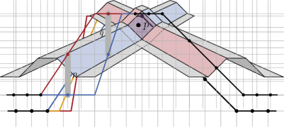
Figure 3: The value of $f(\cdot,\Theta)$ is fixed (black part), except for the segment through data point $p$. The red, orange and blue segments are just three out of uncountably many possibilities. Its slope can be used to encode a real-valued variable.

Linear Dependencies.

The key idea for encoding constraints between variables is that we can “read” the value of a variable using data points. By placing a data point $p$ at a location where several variable gadgets overlap, each of the variable gadgets contributes its part towards fitting $p$. The exact contribution of each variable gadget depends on its slope. Consequently, if one variable gadget contributes more, the others have to proportionally contribute less. This enforces linear dependencies between different variable gadgets and can be used to design addition and copy gadgets.

Figure 4: Two levees, each encoding a variable (slope of the blue and red regions). Point $p$ lies in the intersection and can encode a linear relationship between them.

To be able to intersect multiple variable-encoding gadgets, we need a second input dimension. Each variable-encoding gadget as seen in Figure 3 is now extended into a stripe in $\mathbb{R}^{2}$, with Figure 3 showing only an orthogonal cross section of this stripe. See Figure 4 for two intersecting levees. Much of the technical difficulties lie in the subtleties to enforce the presence of multiple (possibly intersecting) gadgets in $\mathbb{R}^{2}$ using a finite number of data points.

To construct an addition gadget we need to be able to encode linear relations between three variables. In $\mathbb{R}^{2}$, three lines (or stripes) usually do not intersect in a single point. Thus, for addition we introduce three new variable gadgets that are carefully placed to guarantee such a single intersection point. Then we make use of the capability to copy the correct values of the involved variables to the three new variable gadgets. As copying happens at the intersection of only two variable gadgets, this is relatively easy.

Inversion Constraint.

Within only a single output dimension, we are not able to encode nonlinear constraints [ABMM18]. We therefore add a second output dimension, which implies that the neural network represents two functions $f^{1}(\cdot,\Theta)$ and $f^{2}(\cdot,\Theta)$. Consequently, we are allowed to use data points with two different output labels, one for each output dimension.

One important observation is that the locations of breaklines of $f=f(\cdot,\Theta)=(f_{1}(\cdot,\Theta),f_{2}(\cdot,\Theta))$ only depend on the weights and biases in the first layer of the neural network. Thus, every breakline is present in both functions $f^{1}$ and $f^{2}$, except if the corresponding weight to the output neuron is zero. This fact connects the two output dimensions in a way that we can utilize to encode nonlinear constraints.

We define an inversion gadget (realizing the constraint $X\cdot Y=1)$, which also corresponds to a stripe in $\mathbb{R}^{2}$. For simplicity, we again only show a cross section here, see Figure 5. In each output dimension, the inversion gadget looks exactly like the variable gadget. The inversion gadget can therefore be understood as a variable gadget that carries two values.

We prove that by allowing only five breakpoints in total, function $f$ can only fit all data points exactly if $f^{1}$ and $f^{2}$ share three of their four breakpoints with each other (while both having one “exclusive” breakpoint each). This enforces a nonlinear dependency between the slopes of $f^{1}$ and $f^{2}$. By choosing the right parameters, we use this to construct an inversion gadget.

Figure 5: Data points $p$ and $q$ have different labels in the two output dimensions (red in the first dimension and blue in the second dimension). The black parts are the same in both dimensions. The slopes of the red and the blue parts are related via a nonlinear dependency.

2 $\exists\mathbb{R}$-Membership

Membership in $\exists\mathbb{R}$ is already proven by Abrahamsen, Kleist and Miltzow in [AKM21]. For the sake of completeness, while not being too repetitive, we shortly summarize their argument.

Applying a theorem from Erickson, van der Hoog and Miltzow [EvdHM20], $\exists\mathbb{R}$-membership can be shown by describing a polynomial-time real verification algorithm. Such an algorithm gets a Train-F2NN instance $I$ as well as a certificate $\Theta$ consisting of real-valued weights and biases as its input. The instance $I$ consists of a set $D$ of data points, a network architecture and a target error $\gamma$. The algorithm then needs to verify that the neural network described by $\Theta$ fits all data points in $D$ with a total error at most $\gamma$. The real verification algorithm is executed on a real RAM (see [EvdHM20] for a formal definition). Thus, $\exists\mathbb{R}$-membership can be shown just like -membership, the main difference being the underlying machine model (for -membership the verification algorithm must run on a word RAM instead).

A real verification algorithm for Train-F2NN loops over all data points in $D$ and evaluates the function described by the neural network for each of them. As in our case each hidden neuron uses $\mathrm{ReLU}$ as its activation function, each such evaluation takes linear time in the size of the network. The loss function can be computed in polynomial time on the real RAM (see also Definition 2 and the text afterwards).

3 $\exists\mathbb{R}$-Hardness

In this section we present our $\exists\mathbb{R}$-hardness reduction for Train-F2NN. The reduction is mostly geometric, so we start by reviewing the underlying geometry of the two-layer neural networks considered in the paper in Section 3.1. This is followed by a high-level overview of the reduction in Section 3.2 before we describe the gadgets in detail in Section 3.3. Finally, in Section 3.4, we combine the gadgets into the proof of Theorem 3.

3.1 Geometry of Two-Layer Neural Networks

Our reduction below outputs a Train-F2NN instance for a fully connected two-layer neural network $N$ with two input neurons, two output neurons, and $m$ hidden neurons. As defined above, for given weights and biases $\Theta$, the network $N$ realizes a function $f(\cdot,\Theta):\mathbb{R}^{2}\to\mathbb{R}^{2}$. The goal of this Section is to build a geometric understanding of $f(\cdot,\Theta)$. We point the interested reader to these articles [ABMM18, DK22, HBDSS21, MB17, ZNL18] investigating the set of functions exactly represented by different architectures of ReLU networks.

The $i$-th hidden $\mathrm{ReLU}$ neuron $v_{i}$ realizes a function

$$f_{i}:\mathbb{R}^{2} \to\mathbb{R}$$

$$(x_{1},x_{2}) \mapsto\mathrm{ReLU}(a_{1,i}x_{1}+a_{2,i}x_{2}+b_{i})\text{,}$$

where $a_{1,i}$ and $a_{2,i}$ are the edge weights from the first and second input neuron to $v_{i}$ and $b_{i}$ is its bias. We see that $f_{i}$ is a continuous piecewise linear function: If $a_{1,i}=a_{2,i}=0$, then $f_{i}=\max\{b_{i},0\}$ everywhere. Otherwise, the domain $\mathbb{R}^{2}$ is partitioned into two half-planes, touching along a so-called breakline given by the equation $a_{1,i}x_{1}+a_{2,i}x_{2}+b_{i}=0$. The two half-planes are (see Figure 6)

• the inactive region $\{(x_{1},x_{2})\subseteq\mathbb{R}^{2}\mid a_{1,i}x_{1}+a_{2,i}x_{2}+b_{i}\leq 0\}$ in which $f_{i}$ is constantly $0$, and

• the active region $\{(x_{1},x_{2})\subseteq\mathbb{R}^{2}\mid a_{1,i}x_{1}+a_{2,i}x_{2}+b_{i}>0\}$ in which $f_{i}$ is positive and has a constant gradient.

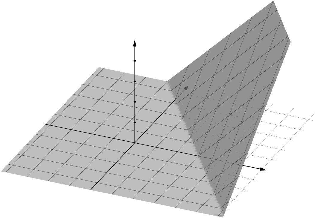
Figure 6: A continuous piecewise linear function computed by a hidden $\mathrm{ReLU}$ neuron. It has exactly one breakline; the left flat part is called the inactive region, whereas the right sloped part is the active region.

Now let $c_{i,1},c_{i,2}$ be the weights of the edges connecting $v_{i}$ with the first and second output neuron, respectively, and let $f(\cdot,\Theta)=(f^{1}(\cdot,\Theta),f^{2}(\cdot,\Theta))$. For $j\in\{1,2\}$, the function $f^{j}(\cdot,\Theta)=\sum_{i=1}^{m}c_{i,j}\cdot f_{i}(\cdot,\Theta)$ is a weighted linear combination of the functions computed at the hidden neurons. We make three observations:

• As each function computed by a hidden $\mathrm{ReLU}$ neuron has at most one breakline, the domain of $f^{j}(\cdot,\Theta)$ is partitioned into the cells of a line arrangement of at most $m$ breaklines. Inside each of these cells $f^{j}(\cdot,\Theta)$ has a constant gradient.

• The position of the breakline that a hidden neuron $v_{i}$ contributes to $f^{j}(\cdot,\Theta)$ is determined solely by the $a_{\cdot,i}$ and $b_{i}$. In particular it is independent of $c_{i,j}$. Thus, the sets of breaklines partitioning $f^{1}(\cdot,\Theta)$ and $f^{2}(\cdot,\Theta)$ are both subsets of the same set: the set of (at most $m$) breaklines determined by the hidden neurons.

• Even if all $m$ hidden neurons compute a function with a breakline, $f^{j}(\cdot,\Theta)$ might have fewer breaklines: It is possible for a breakline to be erased by setting $c_{i,j}=0$, or for breaklines created by different hidden neurons to cancel each other out (producing no breakline) or lie on top of each other (combining multiple breaklines into one). In our reduction, we make use of $c_{i,j}=0$ to erase some breaklines in a single output dimension, but we avoid the other two cases of breaklines combining/canceling.

Note that these observations even imply another, stronger, statement: For each breakline, the change of the gradient of $f(\cdot,\Theta)$ when crossing the line is constant along the whole line (see also [DK22]). This allows to distinguish the following types of breaklines, which will ease our argumentation later.

Definition 6.

A breakline $\ell$ is concave (convex) in $f^{j}(\cdot,\Theta)$, if the restriction of $f^{j}(\cdot,\Theta)$ to any two cells separated by $\ell$ in the breakline arrangement is concave (convex).

The type of a breakline is a tuple $(t_{1},t_{2})\in\{\wedge,0,\vee\}^{2}$ describing whether the breaklineis concave $(\wedge)$, erased $(0)$, or convex $(\vee)$ in $f^{1}(\cdot,\Theta)$ and $f^{2}(\cdot,\Theta)$, respectively.

We have now established a basic geometric understanding of the function $f(\cdot,\Theta)$ computed by the neural network $N$. In our reduction we construct a data set which can be fit by a continuous piecewise linear function with $m$ breaklines if and only if a given ETR-INV instance has a solution. To make sure that the continuous piecewise linear function translates to a solution of the constructed Train-F2NN instance, we need the following observation.

Observation 7.

Let $f:\mathbb{R}^{2}\to\mathbb{R}^{2}$ be a continuous piecewise linear function that can be described via a line arrangement $\mathcal{L}$ of $m$ lines with the following properties:

• In at least one cell of $\mathcal{L}$ the value of $f$ is constantly $(0,0)$.

• For each line $\ell\in\mathcal{L}$ the change of the gradient of $f$ when crossing $\ell$ is constant along $\ell$.

Then there is a fully connected two-layer neural network with $m$ hidden neurons computing $f$.

To see that this observation is true, consider the following construction. For each breakline add a hidden neuron realizing the breakline with the inactive region towards the constant-$(0,0)$ cell, and with the correct change of gradients in each output dimension. It is easy to see that the sum of all these neurons computes $f$. For a precise characterization of the functions representable by 2-layer neural networks with $m$ hidden neurons, we refer to [DK22].

3.2 Reduction Overview

We show $\exists\mathbb{R}$-hardness of Train-F2NN by giving a polynomial-time reduction from ETR-INV to Train-F2NN. ETR-INV is a variant of ETR that is frequently used as a starting point for $\exists\mathbb{R}$-hardness proofs in the literature [AAM22, LMM22, DKMR22, AKM21].

Formally, ETR-INV is a special case of ETR in which the quantifier-free part $\varphi$ of the input sentence $\Phi\equiv\exists X_{1},\ldots,X_{n}\in\mathbb{R}:\varphi(X_{1},\ldots,X_{n})$ is a conjunction (only $\land$ is allowed) of constraints, each of which is either of the form $X+Y=Z$ or $X\cdot Y=1$. Further, $\Phi$ either has no solution or one with all values in $[1/2,2]$.

Theorem 8 ([AAM22, Theorem 3.2]).

ETR-INV is $\exists\mathbb{R}$-complete.

Furthermore, ETR-INV exhibits the same algebraic universality we seek for Train-F2NN:

Theorem 9 ([AM19]).

Let $\alpha$ be an algebraic number. Then there exists an instance of ETR-INV, which has a solution when the variables are restricted to $\mathbb{Q}[\alpha]$, but no solution when the variables are restricted to a field $\mathbb{F}$ that does not contain $\alpha$.

The reduction starts with an ETR-INV instance $\Phi$ and outputs an integer $m$ and a set of $n$ data points such that there is a fully connected two-layer neural network $N$ with $m$ hidden neurons exactly fitting all data points ($\gamma=0$) if and only if $\Phi$ is true. Recall that for fixed weights and biases $\Theta$ the neural network $N$ defines a continuous piecewise linear function $f(\cdot,\Theta):\mathbb{R}^{2}\to\mathbb{R}^{2}$.

For the reduction we define several gadgets representing the variables as well as the linear and inversion constraints of the ETR-INV instance $\Phi$. Strictly speaking, a gadget is defined by a set of data points that need to be fit exactly. These data points serve two tasks: Firstly, most of the data points are used to enforce that $f(\cdot,\Theta)$ has $m$ breaklines with predefined orientations and at almost predefined positions. Secondly, the remaining data points enforce relationships between the exact positions of different breaklines.

Globally, our construction yields $f(x,\Theta)=(0,0)$ for “most” $x\in\mathbb{R}^{2}$. Each gadget consists of a constant number of parallel breaklines (enforced by data points) that lie in a stripe of constant width in $\mathbb{R}^{2}$. Only within these stripes $f(\cdot,\Theta)$ possibly attains non-zero values. Where two or more of these stripes intersect, additional data points can encode relations between the gadgets. The semantic meaning of a gadget is fully determined by the distances between its parallel breaklines. Thus each gadget can be translated and rotated arbitrarily without affecting its meaning.

Simplifications.

Describing all gadgets purely by their data points is tedious and obscures the relatively simple geometry enforced by these data points. We therefore introduce two additional constructs, namely data lines and weak data points, that simplify the presentation. In particular, data lines impose breaklines, which in turn are needed to define gadgets. Weak data points are there to ensure that the gadgets used in the reduction encode variables with bounded range and that we can have features that are only active in one output dimension. How these constructs can be realized with carefully placed data points is deferred to Sections 3.3.5 and 3.3.6.

• A data line $(\ell;y)$ consists of a line $\ell\subseteq\mathbb{R}^{2}$ and a label giving the ground truth value $y\in\mathbb{R}^{2}$. When describing a single gadget, we want that all points $p\in\ell$ are exactly fit, that is, $f(p,\Theta)=y$. As soon as we consider several gadgets, their corresponding stripes in $\mathbb{R}^{2}$ might intersect and we do not require that the data lines are fit correctly inside these intersections. As each data line will be enforced by placing finitely many data points on it, we choose coordinates for these defining data points that do not lie in any of the intersections.

• A weak data point relaxes a regular data point and prescribes only a lower bound on the value of the label. For example, we denote by $(x;y_{1},\geq y_{2})$ that $f^{1}(x,\Theta)=y_{1}$, and $f^{2}(x,\Theta)\geq y_{2}$. Weak data points can have such an inequality label in the first, the second, or both output dimensions.

Global Arrangement of Gadgets.

We describe the global arrangement of the stripes belonging to all the gadgets in Section 3.4. However, in Figure 7 we already provide a rough picture to be kept in mind while we define all the gadgets individually.

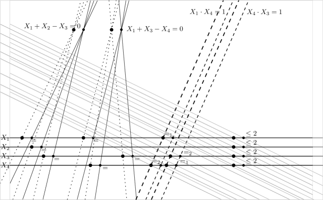
Figure 7: The overall layout of the arrangement of gadgets. The stripes in which the gadgets are defined are simplified to lines for clarity. Our construction contains the following types of gadgets: Variable gadgets (solid, horizontal) representing a value for each variable in the ETR instance, more variable gadgets (dotted) copying these values and realizing addition constraints at their triple intersections, inversion gadgets (dashed) enforcing that two variables fulfill the inversion constraint of the ETR-INV instance, and so-called cancel gadgets (gray, diagonal), which we use to realize weak data points.

3.3 Gadgets and Constraints

We describe all gadgets in isolation first and consider the interaction of two or more gadgets only where it is necessary. In particular, we assume that $f(x,\Theta)$ is constantly zero for $x\in\mathbb{R}^{2}$ outside of the outermost breaklines enforced by each gadget. After all gadgets have been introduced, we describe the global arrangement of the gadgets in Section 3.4. Recall that, since each gadget can be freely translated and rotated, we can describe the positions of all its data lines and (weak) data points relative to each other.

Not all gadgets make use of the two output dimensions. Some gadgets have the same labels in both output dimensions for all of their data lines, and thus look the same in both output dimensions. For these gadgets we simplify the usual notation of $(y_{1},y_{2})\in\mathbb{R}^{2}$ for labels to single-valued labels $y\in\mathbb{R}$. In our figures, data points and functions which look the same in both output dimensions are drawn in black, while features only occurring in one dimension are drawn in orange and blue to distinguish the dimensions from each other.

Let $(\ell_{1},y_{i}),\ldots,(\ell_{k},y_{k})$ be parallel data lines describing (parts of) a gadget and $\ell\subseteq\mathbb{R}^{2}$ be an oriented line intersecting all $\ell_{i}$. Without loss of generality, we assume that the $\ell_{i}$ are numbered such that $\ell_{i}$ intersects $\ell$ before $\ell_{j}$ if and only if $i<j$. Then, this defines a cross section through the gadget: Formally, for each data line $(\ell_{i},y_{i})$ the cross section contains a point $p_{i}=(x_{i},y_{i})\in\mathbb{R}\times\mathbb{R}^{2}$, where $x_{i}$ is the oriented distance between the intersections of $\ell_{1}$ and $\ell_{i}$ on $\ell$. We say that two points $p_{i}$ and $p_{j}$ in the cross section are consecutive, if $|i-j|=1$. If $\ell$ is perpendicular to all $\ell_{i}$, then the cross section is orthogonal.

Each $p_{i}=(x_{i},y_{i})$ in a cross section is a point in $\mathbb{R}\times\mathbb{R}^{2}$. When drawing a cross section in the following figures, we project it into a $2$-dimensional coordinate system by marking $x_{i}$ along the abscissa and $y_{i}$ along the ordinate; if a $y_{i}$ behaves differently in the two output dimensions, we draw it twice distinguishing the two dimensions by color (and clearly marking which two drawn points belong together).

Observation 10.

For a single output dimension, whenever three consecutive points $p_{i},p_{i+1},p_{i+2}$ are not collinear in the cross section, then there must be a breakpoint (the intersection of a breakline $b$ with the cross section) strictly between $p_{i}$ and $p_{i+2}$. Further, if $p_{i+2}$ is above the line through $p_{i}$ and $p_{i+1}$, $b$ must be convex $(\vee)$ in this output dimension. If otherwise $p_{i+2}$ is below that line, $b$ must be concave $(\wedge)$ in this output dimension.

Observation 11.

Whenever three consecutive points $p_{1},p_{i+1},p_{i+2}$ are collinear in one of the two output dimensions, then there is either no breakpoint (active in this dimension) strictly between $p_{i}$ and $p_{i+2}$, or at least two.

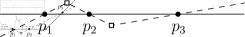
(a) If the points are collinear, then there is either no breakpoint or there are at least two.

(b) If the points are not collinear, then we need a breakpoint of a certain type, here convex.

Figure 8: Three consecutive points $p_{1}$, $p_{2}$ and $p_{3}$ in a cross section and possible interpolations through them (solid and dashed).

Observations 10 and 11 are illustrated in Figure 8. In the analysis of each gadget, we use these observations to prove that the data lines enforce breaklines of a certain type with a prescribed orientation and (almost) fixed position.

3.3.1 Variable Gadget: Levee

Recall that an instance of ETR-INV can be assumed to either have a solution with all variables in $[1/2,2]$ or to have no solution at all. In Train-F2NN, we encode values of variables via a gadget that we call a levee, named after the shape that $f(\cdot,\Theta)$ takes in each output dimension. As mentioned previously, the gadget only affects a stripe of bounded width. See Figure 9 for a cross section view through this stripe.

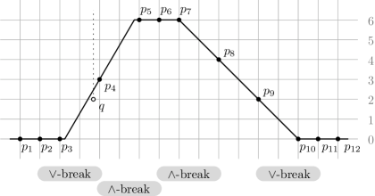
Figure 9: Orthogonal cross section view of a levee. The black points $p_{i}$ are the projections of the data lines $\ell_{1},\ldots,\ell_{12}$, the white point $q$ is a weak data point imposing a lower bound on $f(q,\Theta)$. The bars below the cross section indicate non-collinear triples, where convex (purple) and concave (turquoise) breakpoints are needed. For example, there needs to be a convex breakpoint between $p_{2}$ and $p_{4}$.

A levee consists of four parallel breaklines $b_{1},b_{2},b_{3},b_{4}$, numbered from left to right. Left of $b_{1}$ and right of $b_{4}$ the value of $f(\cdot,\Theta)$ is constantly $0$. Between $b_{2}$ and $b_{3}$ the value of $f(\cdot,\Theta)$ is constantly $6$. The gradient of $f(\cdot,\Theta)$ between $b_{1}$ and $b_{2}$ is orthogonal to the breaklines and oriented towards $b_{2}$. We call the Euclidean norm of the gradient between $b_{1}$ and $b_{2}$ the slope of the levee. The slope $s_{X}$ of a levee for a variable $X$ is at least $3/2$ (if $b_{1}=\ell_{3}$ and $b_{2}=\ell_{5}$) and at most $3$ (if  $f(\cdot,\Theta)$ goes through the lowest possible value for the weak data point $q$). In order to represent values in $[1/2,2]$ we say that a slope $s_{X}$ encodes the value $X=s_{X}-1$.

The gradient between $b_{3}$ and $b_{4}$ carries no semantic meaning. It is merely used to bring $f(\cdot,\Theta)$ back to $0$, such that only a stripe in $\mathbb{R}^{2}$ is affected by the gadget. This part is thus fixed to a slope of $1$ for simplicity.

We realize a levee using twelve parallel data lines, as described in the following table:

	$\ell_{1}$	$\ell_{2}$	$\ell_{3}$	$\ell_{4}$	$\ell_{5}$	$\ell_{6}$	$\ell_{7}$	$\ell_{8}$	$\ell_{9}$	$\ell_{10}$	$\ell_{11}$	$\ell_{12}$
distance to $\ell_{1}$	$0$	$1$	$2$	$4$	$6$	$7$	$8$	$10$	$12$	$14$	$15$	$16$
label	$0$	$0$	$0$	$3$	$6$	$6$	$6$	$4$	$2$	$0$	$0$	$0$

Lemma 12.

Assume that at most four breaklines may be used. Then the twelve parallel data lines $\ell_{1},\ldots,\ell_{12}$ as described in the table above realize a levee with slope in $[3/2,\infty)$, thus carrying a value in $[1/2,\infty)$.

Proof.

We first prove that four breaklines are necessary to fit all data lines exactly. For this, consider an orthogonal cross section through the data lines. It is easy to see that the levee has four non-collinear triples (see Figure 9) and that they pairwise share at most one point. Thus, by Observation 10, four breaklines $b_{1},b_{2},b_{3},b_{4}$ are indeed required.

As $p_{1},p_{2},p_{3}$ are collinear, we can further conclude by Observation 11 that $b_{1}$ has to intersect the cross section at $p_{3}$ or strictly between $p_{3}$ and $p_{4}$. Similarly, as $p_{5},p_{6},p_{7}$ are collinear, we get that $b_{2}$ has to intersect the cross section at $p_{5}$ or strictly between $p_{4}$ and $p_{5}$. The remaining breaklines $b_{3}$ and $b_{4}$ can only intersect the cross section on $p_{7}$ and $p_{10}$, respectively. Since this holds at every orthogonal cross section through the data lines, we further conclude that the breaklines are parallel to each other and to the data lines.

The exact positions of $b_{1}$ and $b_{2}$ depend on each other. As $f(\cdot,\Theta)$ must fit $\ell_{4}$, the distance between $\ell_{4}$ and $b_{1}$ equals the distance between $\ell_{4}$ and $b_{2}$. If $b_{1}=\ell_{3}$ and $b_{2}=\ell_{5}$, the slope of $f(\cdot,\Theta)$ between $b_{1}$ and $b_{2}$ is exactly $3/2$. This is the minimum possible slope, because $\ell_{3}$ and $\ell_{5}$ have to be fit. There is no restriction on the maximum possible slope. Thus $\ell_{1},\ldots,\ell_{12}$ realize a levee carrying a value in $[1/2,\infty)$. ∎

It remains to bound the value of the variable also from above, such that it is constrained to the interval $[1/2,2]$. To achieve this, we use a weak data point, named $q$ in Figure 9. Recall that the label of a weak data point is a lower bound to $f(\cdot,\Theta)$.

Lemma 13.

Let $q$ be a weak data point at distance $3+2/3$ to $\ell_{1}$ (and thus a distance of $1/3$ to $\ell_{4}$) with lower bound label $\geq 2$. Then the slope of the levee is at most $3$.

Proof.

Assume for the sake of contradiction that the slope of $f(\cdot,\Theta)$ between $b_{1}$ and $b_{2}$ is strictly larger than $3$. Then the contribution of the levee to $f(q,\Theta)$ is strictly less than $2$, so the lower bound label of $q$ is not satisfied, a contradiction. ∎

We conclude that with twelve data lines and one weak data point we can enforce four parallel breaklines forming a levee, with a minimum slope of $3/2$ and a maximum slope of $3$, thus encoding a value in the interval $[1/2,2]$.

3.3.2 Measuring a Value from a Levee

A levee represents a value of a variable. For every particular levee we consider the two parallel lines with distance $1$ to $\ell_{4}$ to be its measuring lines. We distinguish the lower measuring line (the one towards $\ell_{3}$) and the upper measuring line (the one towards $\ell_{5}$). Note that, since the slope of the levee is restricted to be in the interval $[3/2,3]$, both measuring lines are always inside or at the boundary of the sloped part (in other words, between breaklines $b_{1}$ and $b_{2}$), see Figure 10.

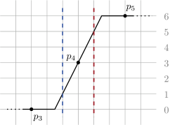
Figure 10: Partial cross section of a levee with slope $s_{X}$ showing the lower (blue) and upper (red) measuring lines. The contribution of this levee at these lines is $3-s_{X}$ and $3+s_{X}$, respectively. As can be seen, this levee has a slope of $s_{X}=2$, thus encoding $X=1$.

Let again $s_{X}$ be the slope of the levee carrying the value of variable $X$. At any point $p$ on $\ell_{4}$, the contribution of the levee to $f(p,\Theta)$ is exactly $3$, assuming $\ell_{4}$ is fit exactly. From this it follows that for a point $p_{u}$ on the upper measuring line the contribution to $f(p_{u},\Theta)$ is $3+s_{X}$. Thus, if we know the value of $f(p_{u},\Theta)$ and further that $p_{u}$ belongs to a single levee only, then we get $X=s_{X}-1=f(p_{u},\Theta)-4$ for the value represented by the levee. Similarly, for a point $p_{l}$ on the lower measuring line the contribution to $f(p_{l},\Theta)$ is $3-s_{X}$. If $p_{l}$ belongs to a single levee only, then $X=s_{X}-1=2-f(p_{l},\Theta)$ is the represented value.

3.3.3 Enforcing Linear Constraints between Variables: Addition and Copying

Until now we always only considered one gadget in isolation. As soon as we have two or more gadgets, their corresponding stripes may intersect. Inside these intersections, the different gadgets interfere and below we describe how to use this interference to encode (non-)linear constraints. Let us note, however, that data lines are not fit correctly inside these intersections any more. This is not a problem because each data line is later replaced by just three collinear data points outside of any intersections of stripes, see Section 3.3.6 below. As we will see there, it is enough that these three data points are fit exactly.

For disjoint subsets $\mathcal{A}$ and $\mathcal{B}$ of the variables we can use an additional data point $p$ to enforce a linear constraint of the form $\sum_{A\in\mathcal{A}}A=\sum_{B\in\mathcal{B}}B$. Note that this type of constraint in particular allows us to copy a value from one levee to another ($X=Y$ via $\mathcal{A}=\{X\},\mathcal{B}=\{Y\}$) or to encode addition ($X+Y=Z$ via $\mathcal{A}=\{X,Y\},\mathcal{B}=\{Z\}$).

The data point $p$ is placed on a measuring line of each involved variable. For all variables in $\mathcal{A}$ the data point $p$ must be on the upper measuring line of the corresponding variable gadget. Similarly, for variables in $\mathcal{B}$ the data point $p$ must be on the lower measuring line. Therefore the levees of the involved variables need to be positioned such that the needed measuring lines all intersect at a common point, where $p$ can be placed. This is trivial for $|\mathcal{A}|+|\mathcal{B}|\leq 2$, see Figure 11; but more involved for more variables, see Figure 12. Using the equality constraint $X=Y$, we can copies the value of a variable onto multiple levees, which can be positioned freely to obtain the required intersections. We discuss the global layout to achieve this in more detail in Section 3.4.

Figure 11: Top-down view on the intersection of two levees corresponding to two variables $X$ (red) and $Y$ (blue). The dashed lines are their measuring lines. The point $p$ is placed at the intersection of the upper measuring line for $X$ and lower measuring line for $Y$, and receives label $6$ to enforce the constraint $X=Y$.

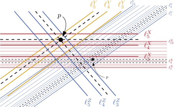
Figure 12: Top-down view of the “interesting part” of the intersection of three levees corresponding to variables $X$ (red), $Y$ (orange), and $Z$ (blue). The dashed lines are upper the measuring lines for $X$ and $Y$ and the lower measuring line for $Z$, intersecting in a single point $p$ with label $10$. This realizes the constraint $X+Y=Z$.

Lemma 14.

The constraint $\sum_{A\in\mathcal{A}}A=\sum_{B\in\mathcal{B}}B$ can be enforced by a data point $p$ placed as described above with label $y=4|\mathcal{A}|+2|\mathcal{B}|$.

Proof.

First, let us consider a variable $A\in\mathcal{A}$ and let $s_{A}$ be the slope of the corresponding levee. Data point $p$ is placed on the upper measuring line of the levee, so it contributes $3+s_{A}$ to $f(p,\Theta)$. Similarly, for a variable $B\in\mathcal{B}$ let $s_{B}$ be the slope of its corresponding levee. Here $p$ is placed on the lower measuring line and this levee contributes $3-s_{B}$ to $f(p,\Theta)$.

The overall contribution of the levees of all involved variables adds up to

$$f(p,\Theta) =\sum_{A\in\mathcal{A}}(3+s_{A})+\sum_{B\in\mathcal{B}}(3-s_{B})$$

$$=\sum_{A\in\mathcal{A}}(4+A)+\sum_{B\in\mathcal{B}}(2-B)\text{,}$$

where we used that the value represented by a levee is its slope minus $1$. Choose the label of $p$ to be $y=4|\mathcal{A}|+2|\mathcal{B}|$. Then, $p$ is fit exactly if and only if the linear constraint $\sum_{A\in\mathcal{A}}A=\sum_{B\in\mathcal{B}}B$ is satisfied. ∎

Lemma 14 is more general than we actually require it for our reduction. The only linear constraint in an instance of ETR-INV is the addition $X+Y=Z$. In our reduction we also need the ability to copy values, i.e., a constraint of the form $X=Y$. These are the only linear constraints required and can be encoded with data points using only two different labels:

Observation 15.

To encode the addition constraint $X+Y=Z$ of ETR-INV the data point has label $10$. For the copy constraint $X=Y$ the data point has label $6$.

Until now we never distinguished between the two output dimensions of levees. Let us note here that it is enough for the data point enforcing the linear constraint to be active in only one output dimension. This holds, because each levee has exactly the same breaklines (and therefore represents the same value) in both output dimensions. In particular, it may also be a weak data point with a lower bound label of $\geq 0$ in the other output dimension. This relaxation is used to realize inversion constraints in the following section.

3.3.4 Inversion Gadget

We introduce an inversion gadget which is in essence the superposition of two levees. This gadget uses data lines with different labels in the two output dimensions to enforce the presence of five parallel breaklines $b_{1},\ldots,b_{5}$, instead of the usual four for a normal levee, see Figure 13. In each output dimension, the continuous piecewise linear function defined by these five breaklines looks like a normal levee, so four of the five breaklines are required. This yields that the two levees in the two output dimensions share three breaklines and have one exclusive breakline each (which is erased in the other output dimension). As for a normal levee, the last two breaklines ($b_{4}$ and $b_{5}$) are just there to bring $f(\cdot,\Theta)$ back to $0$ outside of the stripe of the inversion gadget. In the first output dimension the slope between $b_{1}$ and $b_{2}$ encodes the value while $b_{3}$ is erased. Similarly, in the second output dimension the sloped between $b_{2}$ and $b_{3}$ encodes the value while $b_{1}$ is erased. Note that $b_{2}$ is involved in both sloped parts and therefore changing the value encoded by the levee in one dimension has a directed effect on the value encoded by the levee in the other dimension. As we will see, with carefully placed data lines this dependency encodes an inversion constraint.

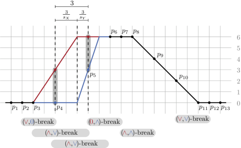
Figure 13: Cross section view of the inversion gadget. The points $p_{1},\ldots,p_{13}$ are the projections of the data lines $\ell_{1},\ldots,\ell_{13}$. Points $p_{4}$ and $p_{5}$ have different labels in the first (red) and second(blue) output dimension. Non-collinear triples of points force breaklines in-between them.

We define an inversion gadget using $13$ parallel data lines, positioned relatively to each other as in the following table:

	$\ell_{1}$	$\ell_{2}$	$\ell_{3}$	$\ell_{4}$	$\ell_{5}$	$\ell_{6}$	$\ell_{7}$	$\ell_{8}$	$\ell_{9}$	$\ell_{10}$	$\ell_{11}$	$\ell_{12}$	$\ell_{13}$
distance to $\ell_{1}$	$0$	$1$	$2$	$4$	$7$	$9$	$10$	$11$	$13$	$15$	$17$	$18$	$19$
label in dim. $1$	$0$	$0$	$0$	$3$	$6$	$6$	$6$	$6$	$4$	$2$	$0$	$0$	$0$
label in dim. $2$	$0$	$0$	$0$	$0$	$3$	$6$	$6$	$6$	$4$	$2$	$0$	$0$	$0$

Lemma 16.

Assume that at most five breaklines may be used. Then the $13$ parallel data lines as described in the table above realize an inversion gadget carrying two values $X$ and $Y$ satisfying $X\cdot Y=1$.

Proof.

Again, we start by showing that at least five breaklines are necessary. First off, there must again be the two fixed breaklines $b_{4}$ and $b_{5}$ on the data lines $\ell_{8}$ and $\ell_{11}$, by the same arguments as for the normal levee (see proof of Lemma 12). There are four more relevant triples of non-collinear points, requiring the following breaklines:

• Triple $p_{2},p_{3},p_{4}$ enforces a $(\vee,0)$-breakline between $\ell_{2}$ and $\ell_{4}$. Actually, since $p_{1},p_{2},p_{3}$ are collinear, the breakline must be between $\ell_{3}$ and $\ell_{4}$.

• Triple $p_{3},p_{4},p_{5}$ enforces a $(\wedge,\vee)$-breakline between $\ell_{3}$ and $\ell_{5}$.

• Triple $p_{4},p_{5},p_{6}$ enforces a $(\wedge,\vee)$-breakline between $\ell_{4}$ and $\ell_{6}$.

• Triple $p_{5},p_{6},p_{7}$ enforces a $(0,\wedge)$-breakline between $\ell_{5}$ and $\ell_{7}$. Actually, since $p_{6},p_{7},p_{8}$ are collinear, the breakline must be between $p_{6}$ and $p_{7}$.

We need to fulfill all four of these requirements with only three remaining breaklines. By looking at the types we see that this is only possible if the triples $p_{3},p_{4},p_{5}$ and $p_{4},p_{5},p_{6}$ enforce the same breakline. This breakline must then be between $\ell_{4}$ and $\ell_{5}$.

As we now know the locations and types of all breaklines, we can analyze the relationship between the values $X$ and $Y$ carried on the two levees. The distance between $\ell_{4}$ and $\ell_{5}$ is $3$ by construction. This distance can be subdivided into the distance from $\ell_{4}$ to $b_{2}$, and from $b_{2}$ to $\ell_{5}$. Between $\ell_{4}$ and $b_{2}$ function $f^{1}(\cdot,\Theta)$ rises from $3$ to $6$, thus the distance between $\ell_{4}$ and $b_{2}$ must be $(6-3)/s_{X}$. Similarly, between $b_{2}$ and $\ell_{5}$ function $f^{2}(\cdot,\Theta)$ rises from $0$ to $3$, thus the distance between $b_{2}$ and $\ell_{5}$ must be $(3-0)/s_{Y}$. These distances add up to $3$, and thus the gadget encodes the constraint $3/s_{X}+3/s_{Y}=3$, or equivalently $3s_{Y}+3s_{X}=3s_{X}s_{Y}$. Using that $X=s_{X}-1$ and $Y=s_{Y}-1$ we get

$$3(Y+1)+3(X+1)=3(X+1)(Y+1)$$

which is true if and only if

$$X\cdot Y=1\text{.}\qed$$

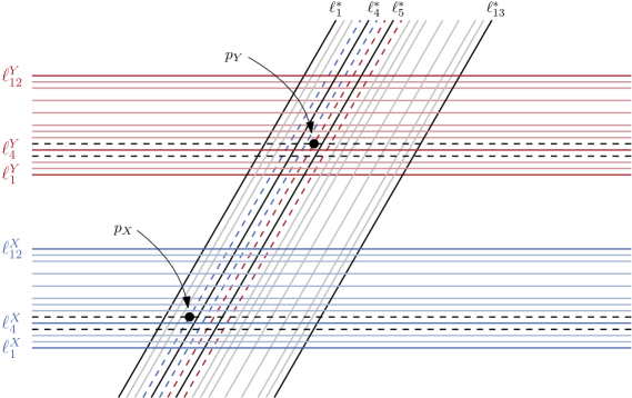
Figure 14: Top-down view on two levees (horizontal), denoted as $X$ (blue) and $Y$ (red) (the data lines are solid and the measuring lines are dashed). The sloped gadget is an inversion gadget linking the two levees. Two weak data points $p_{X}$ and $p_{Y}$ copy $X$ and $Y$ to the first and second dimension of the inversion gadget, respectively.

To encode an $X\cdot Y=1$ constraint of ETR-INV, we first identify two normal levees carrying the variables $X$ and $Y$. Then the inversion gadget is placed so that it intersects both. In the intersection with the $X$-levee we copy $X$ to the first dimension of the inversion gadget and in the intersection with the $Y$-levee we copy $Y$ to the second dimension of the inversion gadget. This copying can be done as described in Section 3.3.3 using weak data points. See Figure 14 for a top-down view on this construction. As levees carry the same value in both output dimensions, enforcing the inversion constraint on just one dimension of each levee ($X$ and $Y$) is sufficient.

Note that the sloped parts of an inversion gadget differ in the two output dimensions. In particular the measuring lines in the first dimension have distance $1$ to $\ell_{4}$, while the measuring lines in the second dimension have distance $1$ to $\ell_{5}$. Thus the weak data points used for copying need to be placed on the measuring lines of the correct dimension.

3.3.5 Realizing Weak Data Points: Cancel Gadgets

Recall that, for our construction so far, we used weak data points with labels of the form $\geq y$ in one or both output dimensions. We now introduce a gadget which can be used to realize such a weak data point using only non-weak data points (with constant labels). For each weak data point $p$ we introduce a cancel gadget, consisting of three parallel breaklines that form a stripe containing $p$ but that shall not contain any other (weak) data point.

A cancel gadget can be active in either one of the two output dimensions, or in both of them. If a cancel gadget is active in some output dimension, the breaklines form a $\vee$ shape of variable height in that dimension. On the other hand, if the cancel gadget is inactive in some output dimension, the breaklines are all inactive (type $0$) and the gadget contributes nothing to $f(\cdot,\Theta)$ in this dimension. The following table shows the locations and labels of the eight data lines that define a cancel gadget. The cancel gadget is illustrated in Figure 15.

	$\ell_{1}$	$\ell_{2}$	$\ell_{3}$	$\ell_{4}$	$\ell_{5}$	$\ell_{6}$	$\ell_{7}$	$\ell_{8}$
distance to $\ell_{1}$	$0$	$1$	$2$	$3$	$5$	$6$	$7$	$8$
label in active dimension(s)	$0$	$0$	$0$	$-1$	$-1$	$0$	$0$	$0$
label in inactive dimension(s)	$0$	$0$	$0$	$0$	$0$	$0$	$0$	$0$

(a) The cancel gadget can be asymmetric.

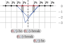
(b) A cancel gadget has a maximum contribution to the weak data point of $-2$.

Figure 15: Cross sections of a cancel gadget which is inactive in the first (red) dimension and active in the second (blue) dimension. It is used to “cancel” a weak data point in the active dimension (blue) that lies on the dashed vertical line. In the inactive dimension (red) it does not contribute anything to $f(\cdot,\Theta)$, i.e., all breaklines are erased (type $0$).

Lemma 17.

Assume that at most three breaklines may be used. The eight data lines as described above realize a cancel gadget that contributes $0$ to $f(p,\Theta)$ in an inactive dimension and an arbitrary amount $c\in(-\infty,-2]$ to $f(p,\Theta)$ in an active dimension to any point $p$ with equal distance to $\ell_{4}$ and $\ell_{5}$.

Proof.

Again we start by arguing that three breaklines are necessary in each active output dimension. There are the following non-collinear triples, each enforcing a breakline:

• Triple $p_{2},p_{3},p_{4}$ enforces a $\wedge$-breakline between $\ell_{2}$ and $\ell_{4}$. Actually, since $p_{1},p_{2},p_{3}$ are collinear, the breakline must be between $\ell_{3}$ and $\ell_{4}$.

• Triple $p_{3},p_{4},p_{5}$ enforces a $\vee$-breakline between $\ell_{3}$ and $\ell_{5}$.

• Triple $p_{4},p_{5},p_{6}$ enforces a $\vee$-breakline between $\ell_{4}$ and $\ell_{6}$.

• Triple $p_{5},p_{6},p_{7}$ enforces a $\wedge$-breakline between $\ell_{5}$ and $\ell_{7}$. Actually, since $p_{6},p_{7},p_{8}$ are collinear, the breakline must be between $\ell_{5}$ and $\ell_{6}$.

We see that the two $\wedge$-breaklines must be in disjoint intervals, so we indeed need two different breaklines. We have one breakline remaining to satisfy the two $\vee$-type enforcements. Thus we get $b_{1}$ of type $\wedge$ between $\ell_{3}$ and $\ell_{4}$, $b_{2}$ of type $\vee$ between $\ell_{4}$ and $\ell_{5}$, and $b_{3}$ of type $\wedge$ between $\ell_{5}$ and $\ell_{6}$. All breaklines must be inactive (type $0$) in an inactive output dimension.

We can now analyze the possible contribution of the cancel gadget in an active output dimension to a point $p$ equidistant to $\ell_{4}$ and $\ell_{5}$. Any contribution $c\in(-\infty,-2]$ can be realized by placing breakline $b_{1}$ at distance $-1/(c+1)$ left of $\ell_{4}$, breakline $b_{3}$ at distance $-1/(c+1)$ right of $\ell_{5}$ and breakline $b_{2}$ equidistant between $\ell_{4}$ and $\ell_{5}$. A contribution $c>-2$ can not be realized, as otherwise there would need to be two convex breaklines, because $p_{3},p_{4},p$ and $p,p_{5},p_{6}$ are both non-collinear triples requiring a convex breakline. ∎

Since the breaklines are at the exact same positions in both output dimensions we can observe the following:

Observation 18.

If the cancel gadget is active in both output dimensions, it contributes the same amount to the weak data point in both dimensions.

The cancel gadget is placed such that the weak data point is equidistant to $\ell_{4}$ and $\ell_{5}$. The inequality label $\geq y$ of the weak data point is converted into the constant label $y-2$.

As shown above, the cancel gadget can contribute any value $c\in(-\infty,-2]$ to the data point. Thus, the data point can be fit perfectly if and only if the other gadgets contribute at least a value of $y$ to the data point, that is, the intended weak constraint is met.

Lastly, let us note that a cancel gadget could also be constructed such that it has a $\wedge$ shape and contributes a positive value in $[2,\infty)$ to the data point. This would allow constraints of the form $\leq y$ as well. Combining two cancel gadgets, one positive and one negative, would even allow a data point to attain an arbitrary value in $\mathbb{R}$ (in one of the two dimensions), but this is not needed for our reduction.

3.3.6 Realizing Data Lines using Data Points

We previously assumed that our gadgets are defined by data lines, but in the Train-F2NN problem, we are only allowed to use data points. In this section, we argue that a set of data lines can be realized by replacing each data line by three data points. This in turn allows us to define the gadgets described throughout previous sections solely using data points. This section is devoted to showing the following lemma, which captures this transformation formally. Note that our replacement of data lines by data points does not work in full generality, but we show it for all the gadgets that we constructed.

Lemma 19.

Assume we are given a set of gadgets (levees, inversion gadgets and cancel gadgets), in total requiring $m$ breaklines. Further assume that the gadgets are placed in $\mathbb{R}^{2}$ such that no two parallel gadgets overlap. Then each data line can be replaced by three data points such that a continuous piecewise linear function with at most $m$ breaklines fits the data points if and only if it fits the data lines.

For the proof consider the line arrangement induced by the data lines. We introduce three vertical lines $v_{1},v_{2},v_{3}$ to the right of all intersections between the data lines. The vertical lines are placed at unit distance to one another. In our construction, no data line is vertical, thus each data line intersects each of the vertical lines exactly once. We place one data point on each intersection of each vertical line with a data line. The new data point inherits the label of the underlying data line. Furthermore, on each vertical line, we ensure that the minimum distance $\alpha$ between any two data points belonging to different gadgets is larger than the maximum distance $w$ between data points belonging to the same gadget. This can be achieved by placing the $v_{1}$, $v_{2}$ and $v_{3}$ far enough to the right and by ensuring a minimum distance between parallel gadgets. See Figure 16 for an illustration.

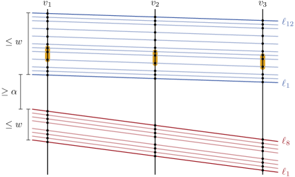
Figure 16: Data lines defining a levee (blue) and a cancel gadget (red) and their intersections with the vertical lines $v_{1},v_{2},v_{3}$. We add a data point at each intersection. The values $\alpha$ and $w$ describe the minimal distance between data lines of different gadgets, and the maximal distance between data lines of the same gadget, respectively. In orange, we highlighted three matching breakpoint intervals (in this case forcing a $\wedge$-breakpoint between $\ell_{4}$ and $\ell_{6}$ of the levee).

Along each of the three vertical lines the data points form cross sections of all the gadgets, similar to the cross sections shown in Figures 9, 13 and 15 (note however that here the cross sections are not orthogonal). We have previously analyzed cross sections of individual gadgets in the proofs of Lemmas 12, 16 and 17. There we identified certain intervals between some of the data lines that need to contain a breakpoint (the intersection of a breakline and the cross section). If we now consider the cross sections of all gadgets along the vertical lines, we refer to these intervals as breakpoint intervals. A breakpoint interval may degenerate to just one point (we have seen this for example for the fixed-slope side of a levee). By our placement of the vertical lines, the cross sections (and thus also the breakpoint intervals) of different gadgets do not overlap.

Any two data lines bounding a breakpoint interval on $v_{1}$ also bound a breakpoint interval on $v_{2}$ and $v_{3}$. We call the three breakpoint intervals on $v_{1}$, $v_{2}$ and $v_{3}$ which are bounded by the same data lines matching breakpoint intervals.

In total there are $3m$ breakpoint intervals. We show that the only way to stab each of them exactly once using $m$ breaklines is if each breakline stabs exactly three matching breakpoint intervals. The first observation towards this is that each breakline can only stab a single breakline interval per vertical line because all breakline intervals are pairwise disjoint. Thus, having $m$ breakpoint intervals on each vertical line, each of the $m$ breaklines has to stab exactly three intervals, one per vertical line. In a first step, we show that each breakline has to stab three breakpoint intervals belonging to the same gadget.

Claim 20.

Each breakline has to stab three breakpoint intervals of the same gadget.

Proof.

The proof is by induction on the number of gadgets. For a single gadget the claim trivially holds. For the inductive step, we consider the lowest gadget $g$ (on $v_{1}$, $v_{2}$ and $v_{3}$) and assume for the sake of contradiction that there is a breakline $b$ stabbing a breakpoint interval of $g$ on $v_{2}$ and a breakpoint interval of a different gadget $g^{\prime}$ above $g$ on $v_{1}$. By construction, the minimum distance $\alpha$ between different gadgets is larger than the maximum width $w$ of any gadget on all three vertical lines. Thus, the distance of any breakpoint interval of $g^{\prime}$ to any breakpoint interval of $g$ on $v_{1}$ is larger than the width of $g$ on $v_{3}$. Therefore, we know that the breakline $b$ intersects $v_{3}$ below any breakpoint intervals of $g$, which is the lowest gadget on $v_{3}$. Thus it stabs at most two breakpoint intervals in total and therefore not all intervals can be stabbed. The same reasoning holds if the roles of $v_{1}$ and $v_{3}$ are flipped. All breaklines stabbing breakpoint intervals of $g$ on $v_{2}$ must therefore also stab breakpoint intervals of $g$ on $v_{1}$ and $v_{3}$. Applying the induction hypothesis on the remaining gadgets, it follows that each breakline only stabs breakpoint intervals of the same gadget. ∎

We can therefore analyze the situation for each gadget in isolation. The main underlying idea is to use the type of the required breakline. Each breaklines must stab three breakpoint intervals of the same type. Let us summarize the findings about required breakline locations and types from the proofs of Lemmas 12, 16 and 17 in Table 1(c).

Table 1: Location and type of the breaklines in levees, inversion gadgets, and cancel gadgets.

	Location	Type
$b_{1}$	$[\ell_{3},\ell_{4})$	$(\vee,\vee)$
$b_{2}$	$(\ell_{4},\ell_{5}]$	$(\wedge,\wedge)$
$b_{3}$	on $\ell_{7}$	$(\wedge,\wedge)$
$b_{4}$	on $\ell_{10}$	$(\vee,\vee)$

(a) Levee

	Location	Type
$b_{1}$	$[\ell_{3},\ell_{4})$	$(\vee,0)$
$b_{2}$	$(\ell_{4},\ell_{5})$	$(\wedge,\vee)$
$b_{3}$	$(\ell_{5},\ell_{6}]$	$(0,\wedge)$
$b_{4}$	on $\ell_{8}$	$(\wedge,\wedge)$
$b_{5}$	on $\ell_{11}$	$(\vee,\vee)$

(b) Inversion gadget.

	Location	Type
$b_{1}$	$[\ell_{3},\ell_{4})$	$(0,\wedge)$
$b_{2}$	$(\ell_{4},\ell_{5})$	$(0,\vee)$
$b_{3}$	$(\ell_{5},\ell_{6}]$	$(0,\wedge)$

(c) Cancel gadget.

Claim 21.

To stab all breakpoint intervals of a levee with only four breaklines, each of them has to stab three matching breakpoint intervals.

Proof.

See Table 1(a). On the three vertical lines, there are six breakpoint intervals for breaklines of type $(\vee,\vee)$ in total. If only two breaklines should stab these six breakpoint intervals, one breakline needs to stab at least two of the single-point intervals. If a breakline goes through two of the single points, it also goes through the third point, and can thus not go through the proper intervals. Therefore one breakline must stab the single-point intervals, and the other one stabs the proper breakpoint intervals.

The same argument can be made for the breakpoint intervals of type $(\wedge,\wedge)$, and thus each breakline stabs three matching breakpoint intervals. ∎

Claim 22.

To stab all breakpoint intervals of an inversion gadget with only five breaklines, each of them has to stab three matching breakpoint intervals.

Proof.

See Table 1(b). All five sets of three matching breakpoint intervals have a different type of required breakline, thus each breakline stabs three matching breakpoint intervals. ∎

Claim 23.

To stab all breakpoint intervals of a cancel gadget with only three breaklines, each of them has to stab three matching breakpoint intervals.

Proof.

See Table 1(c). There is only one set of three breakpoint intervals for a breakline of type $(0,\vee)$, so it is trivially matched correctly.

We can see that the breakpoint intervals for a breakline of type $(0,\wedge)$ have a distance of $2$ from each other, and each have a width of $1$. If the two breaklines of this type would not stab three matching breakpoint intervals, one of them would need to stab two matching intervals and one non-matching interval. As the distance between the vertical lines is equal and the breakpoint intervals are further apart from each other than their width, there is no way for a breakline to lie in this way. We conclude that all breaklines stab three matching breakpoint intervals. ∎

From Claims 21, 22 and 23 it also follows that within a single gadget, between the vertical lines no two breaklines can cross each other, nor can they cross a data line. Together with Claim 20, we can finally prove Lemma 19.

Proof of Lemma 19.

By Claim 20 it follows that every breakline must stab three breakpoint intervals of the same gadget. By Claims 21, 22 and 23 it follows then that each breakline must stab three matching breakpoint intervals, and therefore the breaklines do not cross any data lines between the three vertical lines.

It remains to show that the data points already ensure that each breakline $b$ is parallel to the two parallel data lines $d$ and $d^{\prime}$ enclosing it. To this end, consider the parallelogram defined by $d,d^{\prime},v_{1},v_{3}$ (see Figure 17) and let $j$ be an output dimension in which $b$ is active (not erased). Since no other breakline intersects this parallelogram, we obtain that $f^{j}$ has exactly two linear pieces within the parallelogram, which are separated by $b$. Moreover, since $b$ stabs matching breakpoint intervals, the three data points on $d$ must belong to one of the pieces. Since these points have the same label, it follows that the gradient of this piece in output dimension $j$ must be orthogonal to $d$ (and, thus, to $d^{\prime}$ as well). Applying the same argument on the data points on $d^{\prime}$, we obtain that the gradient of the other piece must be orthogonal to $d$ and $d^{\prime}$ as well. This implies that also the difference of the gradients of the two pieces is orthogonal to $d$ and $d^{\prime}$. Finally, since $b$ must be orthogonal to this difference of gradients, we obtain that it is parallel to $d$ and $d^{\prime}$. ∎

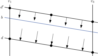
Figure 17: The parallelogram enclosed by the two data lines $d$, $d^{\prime}$ and the vertical lines $v_{1}$, $v_{3}$. The three data points (black) on each data line enforce the gradient in both cells to be orthogonal to the data lines. As a consequence, the breakline $b$ (blue) separating the cells has to be parallel to the data lines.

3.4 Global Construction Layout

We can now finalize proving $\exists\mathbb{R}$ hardness of Train-F2NN For each variable $X$ of the ETR-INV formula, we build a horizontal canonical levee carrying this variable at the bottom of the construction. As argued previously, the levees naturally ensure $X\geq 1/2$ for all variables $X$ and the added weak data point with label $\geq 2$ ensures $X\leq 2$.

The constraints of the form $X+Y=Z$ are enforced by copying the three involved variables onto three new levees. These three new levees are positioned to intersect above all horizontal levees in a way such that their correct measuring lines intersect in a single point. This allows a data point enforcing the constraint to be placed.

For the $k$ inversion constraints of the form $X\cdot Y=1$ we build an array of $k$ parallel inversion gadgets intersecting all canonical levees. Each inversion gadget is connected to the two levees of the variables involved in the constraint (by copying their values into the two dimensions of the inversion gadget).

Finally, we add a cancel gadget for each weak data point such that the cancel gadget contains only this data point but no other data points.

The complete layout can be seen in Figure 18, and an overview over all used gadgets and constructions can be seen in Table 2.

Figure 18: The layout of all gadgets and additional data points for the complete reduction. Each gadget is simplified to a single line for clarity. Solid: Levees. Dashed: Inversion gadgets. Gray: Cancel Gadgets. A point with label $=_{i}$ indicates a copy that is only active in output dimension $i$.

Table 2: An overview of all parts of the construction.

Gadget	#Breaklines	#Data Points	Labels
levee	4	37	$(0,0)$, $(2,2)$, $(3,3)$, $(4,4)$, $(6,6)$
inversion gadget	5	39	$(0,0)$, $(2,2)$, $(0,3)$, $(3,6)$, $(4,4)$, $(6,6)$
addition	0	1	$(10,10)$
copy	0	1	$(-2,6)$, $(6,-2)$, $(6,6)$
cancel gadget	3	24	$(0,0)$, $(0,-1)$, $(-1,0)$, $(-1,-1)$

Proof of Theorem 3.

For $\exists\mathbb{R}$-membership we refer to Section 2. For $\exists\mathbb{R}$-hardness, we reduce from the $\exists\mathbb{R}$-complete problem ETR-INV to Train-F2NN. Given an instance of ETR-INV, we construct an instance of Train-F2NN with $\gamma=0$ as described in the previous paragraphs and shown in Figure 18.

Let $m$ be the minimum number of breaklines needed to realize all gadgets of the above construction: We need four breaklines per levee (Lemma 12), five breaklines per inversion gadget (Lemma 16) and three breaklines per cancel gadget (Lemma 17). We obtain the following chain of equivalences, completing our reduction:

• The ETR-INV instance is a yes-instance.

• There exists a satisfying assignment of the variables of the ETR-INV instance.

• There exists a continuous piecewise linear function fitting all data points of the Train-F2NN instance constructed above and fulfills the conditions of Observation 7 with $m$ breaklines.

• There exists a fully connected two-layer neural network with $m$ hidden $\mathrm{ReLU}$ neurons fitting all the data points.

• The Train-F2NN instance is a yes-instance.

The first and the last equivalence are true by definition.

To see that the second equivalence is true, first assume that there is a satisfying assignment of the variables of the ETR-INV instance. Then these values can be used to find suitable slopes for the levees, inversion gadgets and cancel gadgets in the construction (recall that the slope is the value plus $1$). The superposition of all these gadgets yields the desired continuous piecewise linear function. The function satisfies Observation 7 because, first, the gadgets are built in such a way that functions fitting all data points are constantly zero everywhere except for within the gadgets, and second, the gradient condition is satisfied for each gadget separately and, hence, also for the whole function. For the other direction assume that such a continuous piecewise linear function exists. By Lemmas 19 and 17 the data points enforce exactly the same continuous piecewise linear function as the conceptual data lines and weak data points would. By Lemmas 12, 13 and 16 this continuous piecewise linear function has the shape of the gadgets. Now using that all data points are fit, the slopes of the levees, and inversion gadgets indeed correspond to a satisfying assignment of ETR-INV.

For the third equivalence, Observation 7 guarantees that such a fully connected two-layer neural network with $m$ hidden $\mathrm{ReLU}$ neurons exists. To show the other direction, first note that the function realized by a fully connected two-layer neural network with $m$ hidden $\mathrm{ReLU}$ neurons is always a continuous piecewise linear function with at most $m$ breaklines and satisfying the gradient condition. To see that the other condition of Observation 7 is satisfied, note that the only way to fit all data points with a continuous piecewise linear function of this type is such that it is constantly zero outside all the gadgets.

The Train-F2NN instance can be constructed in polynomial time, as the gadgets can be arranged in such a way that all data points (residing on intersections of lines) have coordinates which can be encoded in polynomial length.

The number of hidden neurons $m$ is linear in the number of variables and the number of constraints of the ETR-INV instance. The number of data points can be bounded by $10m$, thus the number of hidden neurons is linear in the number of data points.

As can be gathered from Table 2, the set of used labels is

$$\{(-2,6),(-1,-1),(-1,0),(0,-1),(0,0),(0,3),(2,2),(3,3),(3,6),(4,4),(6,-2),(6,6),(10,10)\}$$

with cardinality $13$ as claimed. ∎

Note that if the ETR-INV instance is satisfiable, each levee and inversion gadget in a corresponding solution $\Theta$ to the constructed Train-F2NN instance has a slope of at most $3$ in each dimension. Furthermore, no cancel gadget needs to contribute less than $-12$ to satisfy its corresponding weak data point. Thus, there must also be a solution $\Theta^{\prime}$, where each cancel gadget is symmetric, and thus the function $f(\cdot,\Theta^{\prime})$ is Lipschitz continuous with a low Lipschitz constant $L$, which in particular does not depend on the given ETR-INV instance. Checking all the different ways how our gadgets intersect, one can verify that $L=25$ is sufficient.

It remains to prove algebraic universality of Train-F2NN. Intuitively, it suffices to show that the transformations of a solution of an ETR-INV instance to a solution of the corresponding Train-F2NN instance and vice-versa in the above proof of Theorem 3 require only basic field arithmetic, that is, addition, subtraction, multiplication, and division.

Lemma 24.

Let $I$ be an instance of ETR-INV and $N$ be the instance of Train-F2NN built from $I$ by our reduction. We denote by $k$ and $\ell$ the number of variables in a solution of $I$ and $N$ respectively. In ETR-INV, these are the variables $X_{1},\ldots,X_{k}$. In Train-F2NN, these are the weights and biases of the neural network, in some predefined order. The set $V(I)\subseteq\mathbb{R}^{k}$ denotes the set of solutions to $I$, and the set $V(N)\subseteq\mathbb{R}^{\ell}$ denotes the set of solutions to $N$, respectively. Let $\mathbb{F}$ be a field extension of $\mathbb{Q}$. Then,

$$V(I)\cap\mathbb{F}^{k}=\emptyset\Longleftrightarrow V(N)\cap\mathbb{F}^{\ell}=\emptyset\text{.}$$

Proof of Lemma 24.

We first show that $V(N)\cap\mathbb{F}^{\ell}\neq\emptyset$ implies $V(I)\cap\mathbb{F}^{k}\neq\emptyset$: Let $\Theta\in V(N)\cap\mathbb{F}^{\ell}$ be a solution of the Train-F2NN instance $N$. For each variable $X$ of the encoded ETR-INV instance $I$ there is the canonical levee corresponding to $X$ whose slope $s_{X}$ satisfies $X=s_{X}-1$. There is a unique hidden neuron $v_{i}$ contributing the first breakline of that levee. Using the notation from Section 3.1, the slope of this levee is $a_{2,i}\cdot c_{i,1}$, because the levee is horizontal (implying that $a_{1,i}=0$) and its output is equal in both output dimensions (implying $c_{i,1}=c_{i,2}$). Thus, $X=a_{2,i}\cdot c_{i,1}-1$, which is clearly in $\mathbb{F}$. Moreover, the vector of all values of the variables carried on the levee (which is a solution as proven in the proof of Theorem 3) is in $V(I)\cap\mathbb{F}^{k}$, showing that this set is not empty.

We now prove the opposite direction. Let $X_{1},\ldots,X_{n}\in V(I)\cap\mathbb{F}^{k}$ be a solution of the ETR-INV instance $I$. In our reduction, we place our data points on rational coordinates, and thus all implied data lines can be described by equations with rational coefficients. There exists a unique continuous piecewise linear function $f$ which fits these data points, corresponds to the solution $X_{1},\ldots,X_{n}$, and has the property that all cancel gadgets are symmetric. This function can be realized by a fully connected two-layer neural network. All the gradients of linear pieces in this function can be obtained through elementary operations from the values $X_{1},\ldots,X_{n}$ and rational numbers. Furthermore, all breaklines can be described by equations with coefficients derivable from these same numbers. Thus, there exist weights and biases $\Theta\in\mathbb{F}^{\ell}$ for the neural network which realize function $f$. As $\Theta$ realizes $f$, it fits all data points, and thus $\Theta\in V(N)$, showing that $\Theta\in V(N)\cap\mathbb{F}^{\ell}\neq\emptyset$. ∎

Now Theorem 5, the algebraic universality of Train-F2NN, follows directly from the algebraic universality of ETR-INV (Theorem 9) combined with Lemma 24.

References

- [AAM22] Mikkel Abrahamsen, Anna Adamaszek, and Tillmann Miltzow. The Art Gallery Problem is -complete. Journal of the ACM, 69(1):1–70, 2022. doi:10.1145/3486220.
- [ABMM18] Raman Arora, Amitabh Basu, Poorya Mianjy, and Anirbit Mukherjee. Understanding Deep Neural Networks with Rectified Linear Units. In International Conference on Learning Representations (ICLR 2018), 2018.
- [Abr22] Mikkel Abrahamsen. Covering Polygons is Even Harder. In Nisheeth K. Vishnoi, editor, 2021 IEEE 62nd Annual Symposium on Foundations of Computer Science (FOCS), pages 375–386, 2022. doi:10.1109/FOCS52979.2021.00045.
- [ADLD+20] Reyan Ahmed, Felice De Luca, Sabin Devkota, Stephen Kobourov, and Mingwei Li. Graph Drawing via Gradient Descent, . In David Auber and Pavel Valtr, editors, Graph Drawing and Network Visualization (GD 2020), volume 12590 of Lecture Notes in Computer Science, pages 3–17, 2020. doi:10.1007/978-3-030-68766-3_1.
- [AKM21] Mikkel Abrahamsen, Linda Kleist, and Tillmann Miltzow. Training Neural Networks is ER-complete. In Marc A. Ranzato, Alina Beygelzimer, Yann Dauphin, Percy S. Liang, and Jennifer W Vaughan, editors, Advances in Neural Information Processing Systems (NeurIPS 2021), volume 34, 2021.
- [AM19] Mikkel Abrahamsen and Tillmann Miltzow. Dynamic Toolbox for ETRINV. arXiv preprint, 2019. arXiv:1912.08674.
- [AMS20] Mikkel Abrahamsen, Tillmann Miltzow, and Nadja Seiferth. Framework for ER-Completeness of Two-Dimensional Packing Problems. In 2020 IEEE 61st Annual Symposium on Foundations of Computer Science (FOCS), pages 1014–1021, 2020. doi:10.1109/FOCS46700.2020.00098.
- [AZLS19] Zeyuan Allen-Zhu, Yuanzhi Li, and Zhao Song. A Convergence Theory for Deep Learning via Over-Parameterization. In Kamalika Chaudhuri and Ruslan Salakhutdinov, editors, Proceedings of the 36th International Conference on Machine Learning (ICML 2019), volume 97 of Proceedings of Machine Learning Research, pages 242–252, 2019.
- [BC09] Peter Bürgisser and Felipe Cucker. Exotic Quantifiers, Complexity Classes, and Complete Problems. Foundations of Computational Mathematics, 9(2):135–170, 2009. doi:10.1007/s10208-007-9006-9.
- [BDL22] Digvijay Boob, Santanu S. Dey, and Guanghui Lan. Complexity of Training ReLU Neural Network. Discrete Optimization, 44(1), 2022. doi:10.1016/j.disopt.2020.100620.
- [BGKP21] Julius Berner, Philipp Grohs, Gitta Kutyniok, and Philipp Petersen. The Modern Mathematics of Deep Learning. arXiv preprint, 2021. arXiv:2105.04026.
- [BH19] Marie L. T. Berthelsen and Kristoffer A. Hansen. On the Computational Complexity of Decision Problems About Multi-player Nash Equilibria. In Dimitris Fotakis and Evangelos Markakis, editors, International Symposium on Algorithmic Game Theory, volume 11801 of Lecture Notes in Computer Science, pages 153–167, 2019. doi:10.1007/978-3-030-30473-7_11.
- [BH21] Manon Blanc and Kristoffer A. Hansen. Computational Complexity of Multi-player Evolutionarily Stable Strategies. In Rahul Santhanam and Daniil Musatov, editors, Computer Science – Theory and Applications (CSR 2021), volume 12730 of Lecture Notes in Computer Science, pages 1–17, 2021. doi:10.1007/978-3-030-79416-3_1.
- [BJW19] Ainesh Bakshi, Rajesh Jayaram, and David P. Woodruff. Learning Two Layer Rectified Neural Networks in Polynomial Time. In Alina Beygelzimer and Daniel Hsu, editors, Proceedings of the Thirty-Second Conference on Learning Theory (COLT 2019), volume 99 of Proceedings of Machine Learning Research, pages 195–268, 2019.
- [BM16] Vittorio Bilò and Marios Mavronicolas. A Catalog of EXISTS-R-Complete Decision Problems About Nash Equilibria in Multi-Player Games. In Nicolas Ollinger and Heribert Vollmer, editors, 33rd Symposium on Theoretical Aspects of Computer Science (STACS 2016), Leibniz International Proceedings in Informatics (LIPIcs), pages 17:1–17:13, 2016. doi:10.4230/LIPIcs.STACS.2016.17.
- [BM17] Vittorio Bilò and Marios Mavronicolas. Existential-R-Complete Decision Problems about Symmetric Nash Equilibria in Symmetric Multi-Player Games. In Vollmer Heribert and Brigitte Vallée, editors, 34th Symposium on Theoretical Aspects of Computer Science (STACS 2017), volume 66 of Leibniz International Proceedings in Informatics (LIPIcs), pages 13:1–13:14, 2017. doi:10.4230/LIPIcs.STACS.2017.13.
- [BMP18] Daniel Bienstock, Gonzalo Muñoz, and Sebastian Pokutta. Principled Deep Neural Network Training through Linear Programming. arXiv preprint, 2018. arXiv:1810.03218.
- [BSS89] Lenore Blum, Mike Shub, and Steve Smale. On a Theory of Computation and Complexity over the Real Numbers: NP-Completeness, Recursive Functions and Universal Machines. Bulletin of the American Mathematical Society, 21:1–46, 1989. doi:10.1090/S0273-0979-1989-15750-9.
- [Can88] John Canny. Some Algebraic and Geometric Computations in PSPACE. In STOC ’88: Proceedings of the Twentieth Annual ACM Symposium on Theory of Computing, pages 460–467, 1988. doi:10.1145/62212.62257.
- [CFM+18] Jean Cardinal, Stefan Felsner, Tillmann Miltzow, Casey Tompkins, and Birgit Vogtenhuber. Intersection Graphs of Rays and Grounded Segments. Journal of Graph Algorithms and Applications, 22(2):273–294, 2018. doi:10.7155/jgaa.00470.
- [CGKM22] Sitan Chen, Aravind Gollakota, Adam R. Klivans, and Raghu Meka. Hardness of Noise-Free Learning for Two-Hidden-Layer Neural Networks. arXiv preprint, 2022. arXiv:2202.05258.
- [CKM+16] Dmitry Chistikov, Stefan Kiefer, Ines Marusic, Mahsa Shirmohammadi, and James Worrell. On Restricted Nonnegative Matrix Factorization. In Ioannis Chatzigiannakis, Michael Mitzenmacher, Yuval Rabani, and Davide Sangiorgi, editors, 43rd International Colloquium on Automata, Languages, and Programming (ICALP 2016), volume 55 of Leibniz International Proceedings in Informatics (LIPIcs), pages 103:1–103:14, 2016. doi:10.4230/LIPIcs.ICALP.2016.103.
- [CKM22] Sitan Chen, Adam R. Klivans, and Raghu Meka. Learning Deep ReLU Networks Is Fixed-Parameter Tractable. In Nisheeth K. Vishnoi, editor, 2021 IEEE 62nd Annual Symposium on Foundations of Computer Science (FOCS), pages 696–707, 2022. doi:10.1109/FOCS52979.2021.00073.
- [Cyb89] George Cybenko. Approximation by Superpositions of a Sigmoidal Function. Mathematics of Control, Signals and Systems, 2(4):303–314, 1989. doi:10.1007/BF02551274.
- [DFMS22] Argyrios Deligkas, John Fearnley, Themistoklis Melissourgos, and Paul G. Spirakis. Approximating the Existential Theory of the Reals. Journal of Computer and System Sciences, 125:106–128, 2022. doi:10.1016/j.jcss.2021.11.002.
- [DGK+20] Ilias Diakonikolas, Surbhi Goel, Sushrut Karmalkar, Adam R. Klivans, and Mahdi Soltanolkotabi. Approximation Schemes for ReLU Regression. In Jacob Abernethy and Shivani Agarwal, editors, Proceedings of Thirty Third Conference on Learning Theory (COLT 2020), volume 125 of Proceedings of Machine Learning Research, pages 1452–1485, 2020.
- [DHM19] Michael G. Dobbins, Andreas Holmsen, and Tillmann Miltzow. A Universality Theorem for Nested Polytopes. arXiv preprint, 2019. arXiv:1908.02213.
- [DJL+17] Simon S. Du, Chi Jin, Jason D. Lee, Michael I. Jordan, Aarti Singh, and Barnabas Poczos. Gradient Descent Can Take Exponential Time to Escape Saddle Points. In Guyon Isabelle, Ulrike von Luxburg, Samy Bengio, Hanna Wallach, Rob Fergus, S.V.N Vishwanathan, and Roman Garnett, editors, Advances in Neural Information Processing Systems (NIPS 2017), volume 30, 2017.
- [DK22] Steffen Dereich and Sebastian Kassing. On Minimal Representations of Shallow ReLU Networks. Neural Networks, 148:121–128, 2022. doi:10.1016/j.neunet.2022.01.006.
- [DKMR22] Michael G. Dobbins, Linda Kleist, Tillmann Miltzow, and Paweł Rzążewski. Completeness for the Complexity Class and Area-Universality. Discrete & Computational Geometry, 2022. doi:10.1007/s00454-022-00381-0.
- [DLL+19] Simon Du, Jason Lee, Haochuan Li, Liwei Wang, and Xiyu Zhai. Gradient Descent Finds Global Minima of Deep Neural Networks. In Kamalika Chaudhuri and Ruslan Salakhutdinov, editors, Proceedings of the 36th International Conference on Machine Learning (ICML 2019), volume 97 of Proceedings of Machine Learning Research, pages 1675–1685, 2019.
- [DLN+21] Julian D’Costa, Engel Lefaucheux, Eike Neumann, Joël Ouaknine, and James Worrel. On the Complexity of the Escape Problem for Linear Dynamical Systems over Compact Semialgebraic Sets. In Filippo Bonchi and Simon J. Puglisi, editors, 46th International Symposium on Mathematical Foundations of Computer Science (MFCS 2021), volume 202 of Leibniz International Proceedings in Informatics (LIPIcs), pages 33:1–33:21, 2021. doi:10.4230/LIPIcs.MFCS.2021.33.
- [dRdSF+16] Pedro J. de Rezende, Cid C. de Souza, Stephan Friedrichs, Michael Hemmer, Alexander Kröller, and Davi C. Tozoni. Engineering Art Galleries. In Lasse Kliemann and Peter Sanders, editors, Algorithm Engineering: Selected Results and Surveys, volume 9220 of Lecture Notes in Computer Science, pages 379–417. Springer, 1 edition, 2016. doi:10.1007/978-3-319-49487-6.
- [DWX20] Santanu S. Dey, Guany Wang, and Yao Xie. Approximation Algorithms for Training One-Node ReLU Neural Networks. IEEE Transactions on Signal Processing, 68:6696–6706, 2020. doi:10.1109/TSP.2020.3039360.
- [Eri19] Jeff Erickson. Optimal Curve Straightening is -Complete. arXiv preprint, 2019. arXiv:1908.09400.
- [ES16] Ronen Eldan and Ohad Shamir. The Power of Depth for Feedforward Neural Networks. In Vitaly Feldman, Alexander Rakhlin, and Ohad Shamir, editors, 29th Annual Conference on Learning Theory (COLT 2016), volume 49 of Proceedings of Machine Learning Research, pages 907–940, 2016.
- [EvdHM20] Jeff Erickson, Ivor van der Hoog, and Tillmann Miltzow. Smoothing the gap between NP and ER. In 2020 IEEE 61st Annual Symposium on Foundations of Computer Science (FOCS), pages 1022–1033, 2020. doi:10.1109/FOCS46700.2020.00099.
- [FHN22] Vincent Froese, Christoph Hertrich, and Rolf Niedermeier. The Computational Complexity of ReLU Network Training Parameterized by Data Dimensionality. Journal of Artificial Intelligence Research, 74, 2022. doi:10.1613/jair.1.13547.
- [GBB11] Xavier Glorot, Antoine Bordes, and Yoshua Bengio. Deep Sparse Rectifier Neural Networks. In Geoffrey Gordon, David Dunson, and Miroslav Dudík, editors, Proceedings of the Fourteenth International Conference on Artificial Intelligence and Statistics (AISTATS 2011), volume 15 of Proceedings of Machine Learning Research, pages 315–323, 2011.
- [GBC16] Ian Goodfellow, Yoshua Bengio, and Aaron Courville. Deep Learning. MIT Press, 2016. http://www.deeplearningbook.org.
- [GFPC21] Henry Gouk, Eibe Frank, Bernhard Pfahringer, and Michael J. Cree. Regularisation of neural networks by enforcing Lipschitz continuity. Machine Learning, 110(2):393–416, 2021. doi:10.1007/s10994-020-05929-w.
- [GK19] Surbhi Goel and Adam R. Klivans. Learning Neural Networks with Two Nonlinear Layers in Polynomial Time. In Alina Beygelzimer and Daniel Hsu, editors, Proceedings of the Thirty-Second Conference on Learning Theory (COLT 2019), volume 99 of Proceedings of Machine Learning Research, pages 1470–1499, 2019.
- [GKKT17] Surbhi Goel, Varun Kanade, Adam R. Klivans, and Justin Thaler. Reliably Learning the ReLU in Polynomial Time. In Satyen Kale and Ohad Shamir, editors, Proceedings of the 2017 Conference on Learning Theory (COLT 2017), volume 65 of Proceedings of Machine Learning Research, pages 1004–1042, 2017.
- [GKM18] Surbhi Goel, Adam R. Klivans, and Raghu Meka. Learning One Convolutional Layer with Overlapping Patches. In Jennifer Dy and Andreas Krause, editors, Proceedings of the 35th International Conference on Machine Learning (ICML 2018), volume 80 of Proceedings of Machine Learning Research, pages 1783–1791, 2018.
- [GKMR21] Surbhi Goel, Adam R. Klivans, Pasin Manurangsi, and Daniel Reichman. Tight Hardness Results for Training Depth-2 ReLU Networks. In James R. Lee, editor, 12th Innovations in Theoretical Computer Science Conference (ITCS 2021), volume 185 of Leibniz International Proceedings in Informatics (LIPIcs), pages 22:1–22:14, 2021. doi:10.4230/LIPIcs.ITCS.2021.22.
- [GMVY18] Jugal Garg, Ruta Mehta, Vijay V. Vazirani, and Sadra Yazdanbod. -Completeness for Decision Versions of Multi-Player (Symmetric) Nash Equilibria. ACM Transactions on Economics and Computation, 6(1):1:1–1:23, 2018. doi:10.1145/3175494.
- [GR05] Thierry Gensane and Philippe Ryckelynck. Improved Dense Packings of Congruent Squares in a Square. Discrete & Computational Geometry, 34(1):97–109, 2005. doi:10.5555/3115441.3115583.
- [Han19] Boris Hanin. Universal Function Approximation by Deep Neural Nets with Bounded Width and ReLU Activations. Mathematics, 7(10):992:1–9, 2019. doi:10.3390/math7100992.
- [HBDSS21] Christoph Hertrich, Amitabh Basu, Marco Di Summa, and Martin Skutella. Towards Lower Bounds on the Depth of ReLU Neural Networks. In Marc A. Ranzato, Alina Beygelzimer, Yann Dauphin, Percy Liang, and Jennifer W. Vaughan, editors, Advances in Neural Information Processing Systems (NeurIPS 2021), volume 34, 2021.
- [HHL23] Christian Haase, Christoph Hertrich, and Georg Loho. Lower bounds on the depth of integral ReLU neural networks via lattice polytopes. In Submitted to The Eleventh International Conference on Learning Representations, 2023. Under review. URL: https://openreview.net/forum?id=2mvALOAWaxY.
- [HM21] Simon B. Hengeveld and Tillmann Miltzow. A Practical Algorithm with Performance Guarantees for the Art Gallery Problem. In Kevin Buchin and Éric Colin de Verdière, editors, 37th International Symposium on Computational Geometry (SoCG 2021), volume 189 of Leibniz International Proceedings in Informatics (LIPIcs), pages 44:1–44:16, 2021. doi:10.4230/LIPIcs.SoCG.2021.44.
- [Hor91] Kurt Hornik. Approximation Capabilities of Multilayer Feedforward Networks. Neural Networks, 4(2):251–257, 1991. doi:10.1016/0893-6080(91)90009-T.
- [HR19] Boris Hanin and David Rolnick. Complexity of Linear Regions in Deep Networks. In Kamalika Chaudhuri and Ruslan Salakhutdinov, editors, Proceedings of the 36th International Conference on Machine Learning (ICML 2019), volume 97 of Proceedings of Machine Learning Research, pages 2596–260, 2019.
- [HS18] Boris Hanin and Mark Sellke. Approximating Continuous Functions by ReLU Nets of Minimal Width. arXiv preprint, 2018. arXiv:1710.11278.
- [HS21] Christoph Hertrich and Leon Sering. ReLU Neural Networks of Polynomial Size for Exact Maximum Flow Computation. arXiv preprint, 2021. arXiv:2102.06635.
- [JGH18] Arthur Jacot, Franck Gabriel, and Clément Hongler. Neural Tangent Kernel: Convergence and Generalization in Neural Networks. In Samy Bengio, Hanna Wallach, Hugo Larochelle, Kristen Grauman, Nicolò Cesa-Bianchi, and Roman Garnett, editors, Advances in Neural Information Processing Systems (NeurIPS 2018), volume 31, 2018.
- [JKM22] Paul Jungeblut, Linda Kleist, and Tillmann Miltzow. The Complexity of the Hausdorff Distance. In Xavier Goaoc and Michael Kerber, editors, 38th International Symposium on Computational Geometry (SoCG 2022), volume 224 of Leibniz International Proceedings in Informatics (LIPIcs), pages 48:1–48:17, 2022. doi:10.4230/LIPIcs.SoCG.2022.48.
- [KB22] Sammy Khalife and Amitabh Basu. Neural networks with linear threshold activations: structure and algorithms. In Karen Aardal and Laura Sanità, editors, International Conference on Integer Programming and Combinatorial Optimization (IPCO 2022), volume 13265 of Lecture Notes in Computer Science, pages 347–360, 2022. doi:10.1007/978-3-031-06901-7_26.
- [KM94] Jan Kratochvíl and Jiří Matoušek. Intersection Graphs of Segments. Journal of Combinatorial Theory, Series B, 62(2):289–315, 1994. doi:10.1006/jctb.1994.1071.
- [KM12] Ross Kang and Tobias Müller. Sphere and Dot Product Representations of Graphs. Discrete & Computational Geometry, 47(3):548–569, 2012. doi:10.1007/s00454-012-9394-8.
- [LMM22] Anna Lubiw, Tillmann Miltzow, and Debajyoti Mondal. The Complexity of Drawing a Graph in a Polygonal Region. Journal of Graph Algorithms and Applications, 26(4):421–446, 2022. doi:10.7155/jgaa.00602.
- [LS17] Shiyu Liang and Rayadurgam Srikant. Why Deep Neural Networks for Function Approximation? In International Conference on Learning Representations (ICLR 2017), 2017.
- [Mat14] Jiří Matoušek. Intersection graphs of segments and . arXiv preprint, 2014. arXiv:1406.2636.
- [MB17] Anirbit Mukherjee and Amitabh Basu. Lower bounds over Boolean inputs for deep neural networks with ReLU gates. arXiv preprint, 2017. arXiv:1711.03073.
- [MM13] Colin McDiarmid and Tobias Müller. Integer realizations of disk and segment graphs. Journal of Combinatorial Theory, Series B, 103(1):114–143, 2013. doi:10.1016/j.jctb.2012.09.004.
- [Mnë88] Nikolai E. Mnëv. The Universality Theorems on the Classification Problem of Configuration Varieties and Convex Polytopes Varieties. In Oleg Y. Viro and Anatoly M Vershik, editors, Topology and Geometry — Rohlin Seminar, volume 1346 of Lecture Notes in Mathematics, pages 527–543. Springer, 1988. doi:10.1007/BFb0082792.
- [MPCB14] Guido F. Montúfar, Razvan Pascanu, Kyunghyun Cho, and Yoshua Bengio. On the Number of Linear Regions of Deep Neural Networks. In Zoubin Ghahramani, Max Welling, Corinna Cortes, Neil Lawrence, and Weinberger Kilian Q., editors, Proceedings of the 27th International Conference on Neural Information Processing Systems (NeurIPS 2014), volume 2, pages 2924–2932, 2014.
- [MRZ21] Guido Montúfar, Yue Ren, and Leon Zhang. Sharp bounds for the number of regions of maxout networks and vertices of Minkowski sums. arXiv preprint, 2021. arXiv:2104.08135.
- [MS22] Tillmann Miltzow and Reinier F. Schmiermann. On Classifying Continuous Constraint Satisfaction Problems. In Nisheeth K. Vishnoi, editor, 2021 IEEE 62nd Annual Symposium on Foundations of Computer Science (FOCS), pages 781–791, 2022. doi:10.1109/FOCS52979.2021.00081.
- [NMH18] Quynh Nguyen, Mahesh Chandra Mukkamala, and Matthias Hein. Neural Networks Should Be Wide Enough to Learn Disconnected Decision Regions. In Jennifer Dy and Andreas Krause, editors, Proceedings of the 35th International Conference on Machine Learning (ICML 2018), volume 80 of Proceedings of Machine Learning Research, pages 3740–3749, 2018.
- [PMB14] Razvan Pascanu, Guido Montúfar, and Yoshua Bengio. On the number of response regions of deep feed forward networks with piece-wise linear activations. In International Conference on Learning Representations (ICLR 2014), 2014.
- [RGZ95] Jürgen Richter-Gebert and Günter M. Ziegler. Realization Spaces of 4-Polytopes are Universal. Bulletin of the American Mathematical Society, 32(4):403–412, 1995. doi:10.1090/S0273-0979-1995-00604-X.
- [Ric69] Daniel Richardson. Some Undecidable Problems Involving Elementary Functions of a Real Variable. The Journal of Symbolic Logic, 33(4):514–520, 1969. doi:10.2307/2271358.
- [RPK+17] Maithra Raghu, Ben Poole, Jon Kleinberg, Surya Ganguli, and Jascha Sohl Dickstein. On the Expressive Power of Deep Neural Networks. In Doina Precup and Yee Whye Teh, editors, Proceedings of the 34th International Conference on Machine Learning (ICML 2017), volume 70 of Proceedings of Machine Learning Research, pages 2847–2854, 2017.
- [Sch10] Marcus Schaefer. Complexity of Some Geometric and Topological Problems. In David Eppstein and Emden R. Gansner, editors, GD 2009: Graph Drawing, volume 5849 of Lecture Notes in Computer Science, pages 334–344, 2010. doi:10.1007/978-3-642-11805-0_32.
- [Sch13] Marcus Schaefer. Realizability of Graphs and Linkages, pages 461–482. Thirty Essays on Geometric Graph Theory. Springer, 2013. doi:10.1007/978-1-4614-0110-0_24.
- [Sch21] Marcus Schaefer. Complexity of Geometric k-Planarity for Fixed k. Journal of Graph Algorithms and Applications, 25(1):29–41, 2021. doi:10.7155/jgaa.00548.
- [Shi16] Yaroslav Shitov. A Universality Theorem for Nonnegative Matrix Factorizations. arXiv preprint, 2016. arXiv:1606.09068.
- [Shi17] Yaroslav Shitov. The complexity of positive semidefinite matrix factorization. SIAM Journal on Optimization, 27(3):1898–1909, 2017. doi:10.1137/16M1080616.
- [Sho91] Peter W. Shor. Stretchability of Pseudolines is NP-Hard. In Peter Gritzmann and Bernd Sturmfels, editors, Applied Geometry And Discrete Mathematics, volume 4 of DIMACS Series in Discrete Mathematics and Theoretical Computer Science, pages 531–554, 1991. doi:10.1090/dimacs/004/41.
- [SS17a] Itay Safran and Ohad Shamir. Depth-Width Tradeoffs in Approximating Natural Functions with Neural Networks. In Doina Precup and Yee Whye Teh, editors, Proceedings of the 34th International Conference on Machine Learning (ICML 2017), volume 70 of Proceedings of Machine Learning Research, pages 2979–2987, 2017.
- [SŠ17b] Marcus Schaefer and Daniel Štefankovič. Fixed Points, Nash Equilibria, and the Existential Theory of the Reals. Theory of Computing Systems, 60:172–193, 2017. doi:10.1007/s00224-015-9662-0.
- [SŠ22] Marcus Schaefer and Daniel Štefankovič. Beyond the Existential Theory of the Reals. arXiv preprint, 2022. arXiv:2210.00571.
- [SSBD14] Shai Shalev-Shwartz and Shai Ben-David. Understanding Machine Learning: From Theory to Algorithms. Cambridge University Press, 2014. doi:10.1017/CBO9781107298019.
- [Sta22] Jack Stade. Complexity of the Boundary-Guarding Art Gallery Problem. arXiv preprint, 2022. arXiv:2210.12817.
- [STR18] Thiago Serra, Christian Tjandraatmadja, and Srikumar Ramalingam. Bounding and Counting Linear Regions of Deep Neural Networks. In Jennifer Dy and Andreas Krause, editors, Proceedings of the 35th International Conference on Machine Learning (ICML 2018), volume 80 of Proceedings of Machine Learning Research, pages 4558–4566, 2018.
- [Sv18] Marcus Schaefer and Daniel Štefankovič. The Complexity of Tensor Rank. Theory of Computing Systems, 62(5):1161–1174, 2018. doi:10.1007/s00224-017-9800-y.
- [Tel15] Matus Telgarsky. Representation Benefits of Deep Feedforward Networks. arXiv preprint, 2015. arXiv:1509.08101.
- [Tel16] Matus Telgarsky. Benefits of depth in neural networks. In Vitaly Feldman, Alexander Rakhlin, and Ohad Shamir, editors, 29th Annual Conference on Learning Theory (COLT 2016), volume 49 of Proceedings of Machine Learning Research, pages 1517–1539, 2016.
- [Val84] Leslie G. Valiant. A Theory of the Learnable. Communications of the ACM, 27(11):1134–1142, 1984. doi:10.1145/1968.1972.
- [VYS21] Gal Vardi, Gilad Yehudai, and Ohad Shamir. On the Optimal Memorization Power of ReLU Neural Networks. arXiv preprint, 2021. arXiv:2110.03187.
- [Yar17] Dmitry Yarotsky. Error bounds for approximations with deep ReLU networks. Neural Networks, 94:103–114, 2017. doi:10.1016/j.neunet.2017.07.002.
- [YSJ19] Chulhee Yun, Suvrit Sra, and Ali Jadbabaie. Small ReLU networks are powerful memorizers: a tight analysis of memorization capacity. In Hanna Wallach, Hugo Larochelle, Alina Beygelzimer, Florence d’Alché Buc, Emily Fox, and Roman Garnett, editors, Advances in Neural Information Processing Systems (NeurIPS 2019), volume 32, 2019.
- [ZBH+21] Chiyuan Zhang, Samy Bengio, Moritz Hardt, Benjamin Recht, and Oriol Vinyals. Understanding Deep Learning (Still) Requires Rethinking Generalization. Communications of the ACM, 64(3):107–115, 2021. doi:10.1145/3446776.
- [ZNL18] Liwen Zhang, Gregory Naitzat, and Lek-Heng Lim. Tropical Geometry of Deep Neural Networks. In Jennifer Dy and Andreas Krause, editors, Proceedings of the 35th International Conference on Machine Learning (ICML 2018), volume 80 of Proceedings of Machine Learning Research, pages 5824–5832, 2018.