mVEM: A MATLAB Software Package for the Virtual Element Methods

Abstract

This paper summarizes the development of mVEM, a MATLAB software package containing efficient and easy-following codes for various virtual element methods (VEMs) published in the literature. We explain in detail the numerical implementation of the mixed VEMs for the Darcy problem and the three-dimensional linear VEMs for the Poisson equation. For other model problems, we present the construction of the discrete methods and only provide the implementation of the elliptic projection matrices. Some mesh related functions are also given in the package, including the mesh generation and refinement in two or three dimensions. mVEM is free and open source software.

Keywords. Virtual element method, Polygonal meshes, Three dimensions, MATLAB

1 Introduction

Developing the mimetic finite difference methods, Beirão and Brezzi et al. proposed the virtual element method (VEM) in 2013, and established an abstract framework for error analysis [7]. This method was further studied in [2] for an extension to reaction-diffusion problems, where a crucial enhancement technique is introduced to construct a computable $L^{2}$ projection. The computer implementation has been further studied in [11]. The proposed finite dimensional space in [7] has become the standard space for constructing conforming virtual element methods for second-order elliptic problems on polygonal meshes. The word virtual comes from the fact that no explicit knowledge of the basis functions is necessary since the shape functions are piecewise continuous polynomials on the boundary of the element and are extended to the interior by assuming basis functions as solutions of local Laplace equations. The construction of the VEMs for elliptic problems is very natural and standard, which can be derived based on an integration by parts formula for the underlying differential operator. As a matter of fact, this idea is used to devise conforming and nonconforming VEMs for arbitrary order elliptic problems though the resulting formulation and theoretical analysis are rather involved [39, 27].

VEMs have some advantages over standard finite element methods. For example, they are more convenient to handle partial differential equations on complex geometric domains or the ones associated with high-regularity admissible spaces. Until now, they have been successfully applied to solve various mathematical physical problems, such as the conforming and nonconforming VEMs for second-order elliptic equations [2, 7, 6, 25] and fourth-order elliptic equations [23, 30, 3, 56], the time-dependent problems [47, 46, 43, 1, 36], the mixed formulation of the Darcy and Stokes problems [22, 17, 57] and the variational inequalities and hemivariational inequalities associated with the frictional contact problems [48, 50, 51, 49].

For second-order problems with variable coefficients and convection terms, direct use of the elliptic projection approximation of the gradient operator does not ensure the optimal convergence, so the external projection approximation has been introduced in the literature, see [13, 14] for example. This approximation technique is also commonly used for the construction of virtual element methods for complex problems such as elastic or inelastic mechanics [10, 4, 5]. Since the virtual element space contains at least $k$-th order polynomials, the number of the degrees of freedom (d.o.f.s) in the virtual element space is generally higher than that in the classical finite element space when the polygonal element is degenerated into a triangle. These extra d.o.f.s are usually caused by internal moments and can be further reduced by exploiting the idea of building an incomplete finite element or the serendipity finite element [21]. In fact, Beirão et al. has proposed the serendipity nodal VEM spaces in [12].

In this paper, we are intended to develop a MATLAB software package for the VEMs in two or three dimensions, containing efficient and easy-following codes for various VEMs published in the literature. In particular, [11] provided a detailed explanation of the formulation of the terms in the matrix equations for the high order virtual element method applied to such a problem in two dimensions, and [44] presented a transparent MATLAB implementation of the conforming linear virtual element method for the Poisson equation in two dimensions. The construction of the VEMs for three-dimensional problems has been accomplished in many papers [35, 34, 28, 15, 9, 16, 31]. However, to the best of knowledge, no related implementation is publicly available in the literature. As an extension of [44] to three spatial dimensions, we have provided a clear and useable MATLAB implementation of the method for three-dimensional linear VEMs for the Poisson equation on general polyhedral meshes in the package with the detailed implementation given in Section 10. Although the current procedure is only for first-order virtual element spaces, the design idea can be directly generalized to higher-order cases.

The paper is organized as follows. In Section 2, we provide the complete and detailed implementation of the mixed VEMs for the Darcy problem as an example, which includes almost all of the programming techniques in mVEM, such as the construction of the data structure for polygonal meshes, the computation of elliptic and $L^{2}$ projection matrices, the treatment of boundary conditions, and examples that demonstrate the usage of running the codes, showing the solutions and meshes, computing the discrete errors and displaying the convergence rates. Section 3 summarizes the mesh related built-in functions, including the modified version of PolyMesher introduced in [45] and generation of some special meshes for VEM tests. We also provide the generation of polygonal meshes by establishing the dual mesh of a Delaunay triangulation and some basic functions to show the polygonal meshes as well as a boundary setting function to identify the Neumann and Dirichlet boundaries. Sections 4-9 discuss the construction of virtual element methods for various model problems and the computation of the corresponding elliptical projections, including the conforming and nonconforming VEMs for the Poisson equation or reaction-diffusion problems, the (locking-free) VEMs for the linear elasticity problems in the displacement/tensor type, three VEMs for the fourth-order plate bending problems, the divergence-free mixed VEMs for the Stokes problems, the adaptive VEMs for the Poisson equation and the variational inequalities for the simplified friction problem. The paper ends with some concluding remarks in Section 11.

2 Mixed VEMs for the Darcy problem

Considering that the implementation of conforming or nonconforming VEMs has been publicly available in the literature [44, 42], we in this paper present the detailed implementation of the mixed VEMs for the Darcy problem to fill the gap in this regard. The mixed VEM is first proposed in [22] for the classical model problem of Darcy flow in a porous medium. Let’s briefly review the method in this section.

2.1 Construction of the mixed VEMs

2.1.1 The model problem

Given the (polygonal) computational domain $\Omega\subset\mathbb{R}^{2}$, let $f\in L^{2}(\Omega)$ and $g\in H^{1/2}(\partial\Omega)$. The Darcy problem is to find $p\in H^{1}(\Omega)$ such that

$$\begin{cases}-{\rm div}(\mathbb{K}\nabla p)=f\quad&\mbox{in}~{}~{}\Omega,\\ (\mathbb{K}\nabla p)\cdot\boldsymbol{n}=g\quad&\mbox{on}~{}~{}\partial\Omega,\end{cases}$$ (1)

where $\mathbb{K}$ is a symmetric and positive definite tensor of size $2\times 2$. For simplicity, we assume that $\mathbb{K}$ is constant. The given data $f$ and $g$ satisfy the compatibility condition

$$\int_{\Omega}f{\rm d}x=\int_{\partial\Omega}g{\rm d}s.$$

To remove an additive constant, we additionally require that

$$\int_{\Omega}p{\rm d}x=0.$$ (2)

Introducing the velocity variable $\boldsymbol{u}=\mathbb{K}\nabla p$, the above problem can be rewritten in the mixed form

$$\begin{cases}\boldsymbol{u}=\mathbb{K}\nabla p\quad&\mbox{in}~{}~{}\Omega,\\ {\rm div}\boldsymbol{u}=-f\quad&\mbox{in}~{}~{}\Omega,\\ \boldsymbol{u}\cdot\boldsymbol{n}=g\quad&\mbox{on}~{}~{}\partial\Omega.\end{cases}$$

Define

$$V_{g}=\{\boldsymbol{u}\in H({\rm div};\Omega):\boldsymbol{u}\cdot\boldsymbol{n}=g~{}~{}\mbox{on}~{}~{}\partial\Omega\},\qquad Q=L_{0}^{2}(\Omega),\qquad V=V_{0}.$$

The corresponding mixed variational problem is: Find $(\boldsymbol{u},p)\in V_{g}\times Q$ such that

$$\begin{cases}a(\boldsymbol{u},\boldsymbol{v})+b(\boldsymbol{v},p)&=0,\quad\boldsymbol{v}\in V,\\ b(\boldsymbol{u},q)&=-(f,q),\quad q\in Q,\end{cases}$$ (3)

where

$$a(\boldsymbol{u},\boldsymbol{v})=(\mathbb{K}^{-1}\boldsymbol{u},\boldsymbol{v}),\qquad b(\boldsymbol{v},q)=({\rm div}\boldsymbol{v},q).$$

Note that the boundary condition is now related to the variable $\boldsymbol{u}$.

2.1.2 The virtual element space and the elliptic projection

The local virtual element space of $V$ is

$$V_{k}(K) =\{\boldsymbol{v}\in H({\rm div};K)\cap H({\rm rot};K):\boldsymbol{v}\cdot\boldsymbol{n}|_{e}\in\mathbb{P}_{k}(e),$$

$$\hskip 85.35826pt{\rm div}\boldsymbol{v}|_{K}\in\mathbb{P}_{k-1}(K),~{}~{}{\rm rot}\boldsymbol{v}|_{K}\in\mathbb{P}_{k-1}(K)\},$$ (4)

where

$${\rm div}\boldsymbol{v}=\partial_{1}v_{1}+\partial_{2}v_{2},\quad{\rm rot}\boldsymbol{v}=\partial_{1}v_{2}-\partial_{2}v_{1},\quad\boldsymbol{v}=(v_{1},v_{2})^{T}.$$

To present the degrees of freedom (d.o.f.s), we introduce a scaled monomial $\mathbb{M}_{r}(D)$ on a $d$-dimensional domain $D$

$$\mathbb{M}_{r}(D):=\Big{\{}\Big{(}\frac{\boldsymbol{x}-\boldsymbol{x}_{D}}{h_{D}}\Big{)}^{\boldsymbol{s}},\quad|\boldsymbol{s}|\leq r\Big{\}},$$

where $h_{D}$ is the diameter of $D$, $\boldsymbol{x}_{D}$ the centroid of $D$, and $r$ a non-negative integer. For the multi-index ${\boldsymbol{s}}\in{\mathbb{N}^{d}}$, we follow the usual notation

$$\boldsymbol{x}^{\boldsymbol{s}}=x_{1}^{s_{1}}\cdots x_{d}^{s_{d}},\quad|\boldsymbol{s}|=s_{1}+\cdots+s_{d}.$$

Conventionally, $\mathbb{M}_{r}(D)=\{0\}$ for $r\leq-1$.

The d.o.f.s can be given by

$$\int_{e}\boldsymbol{v}\cdot\boldsymbol{n}q{\rm d}s,\quad q\in\mathbb{M}_{k}(e),~{}~{}e\subset\partial K,$$ (5)

$$\int_{K}\boldsymbol{v}\cdot\nabla q{\rm d}x,\quad q\in\mathbb{M}_{k-1}(K)\backslash\{1\},$$ (6)

$$\int_{K}{\rm rot}\boldsymbol{v}q{\rm d}x,\quad q\in\mathbb{M}_{k-1}(K).$$ (7)

We remark that the moments on edges or elements are not divided by $|e|$ or $|K|$ since $a^{K}(\cdot,\cdot)$ is associated with the $L^{2}$ norm rather than the $H^{1}$ semi-norm for the case of Poisson equation.

For the Poisson equation, the elliptic projection maps from the virtual element space $V_{k}(K)$ into the polynomial space $\mathbb{P}_{k}(K)$ [7, 2, 11]. For convenience, the image space is referred to as the elliptic projection space. For the Darcy problem, however, the elliptic projection space is now replaced by

$$\widehat{V}_{k}(K)=\{\widehat{\boldsymbol{v}}\in V_{k}(K):\widehat{\boldsymbol{v}}=\mathbb{K}\nabla\widehat{q}_{k+1}~{}~{}\mbox{for some}~{}~{}\widehat{q}_{k+1}\in\mathbb{P}_{k+1}(K)\}.$$

The elliptic projector $\widehat{\Pi}^{K}:V_{k}(K)\to\widehat{V}_{k}(K)$, $\boldsymbol{v}\mapsto\widehat{\Pi}^{K}\boldsymbol{v}$ is then defined by

$$a^{K}(\widehat{\Pi}^{K}\boldsymbol{v},\widehat{\boldsymbol{w}})=a^{K}(\boldsymbol{v},\widehat{\boldsymbol{w}}),\quad\widehat{\boldsymbol{w}}\in\widehat{V}_{k}(K).$$ (8)

We now consider the computability of the elliptic projection. In view of the symmetry of $\mathbb{K}$, the integration by parts gives

$$a^{K}(\boldsymbol{v},\widehat{\boldsymbol{w}}) =\int_{K}\mathbb{K}^{-1}\boldsymbol{v}\cdot\widehat{\boldsymbol{w}}{\rm d}x=\int_{K}\boldsymbol{v}\cdot(\mathbb{K}^{-1}\widehat{\boldsymbol{w}}){\rm d}x$$

$$=\int_{K}\boldsymbol{v}\cdot\nabla\widehat{q}_{k+1}{\rm d}x=-\int_{K}\widehat{q}_{k+1}{\rm div}\boldsymbol{v}{\rm d}x+\int_{\partial K}\widehat{q}_{k+1}\boldsymbol{v}\cdot\boldsymbol{n}{\rm d}s.$$ (9)

• For the second term, since $\boldsymbol{v}\cdot\boldsymbol{n}|_{e}\in\mathbb{P}_{k}(e)$ we expand it in the scaled monomials on $e$ as

  $$\boldsymbol{v}\cdot\boldsymbol{n}|_{e}(s)=c_{1}m_{1}^{e}(s)+\cdots+c_{n}m_{n}^{e}(s).$$

  Clearly, the coefficients are uniquely determined by the d.o.f.s in (5).

• For the first term, noting that ${\rm div}\boldsymbol{v}|_{K}\in\mathbb{P}_{k-1}(K)$, we have

  $${\rm div}\boldsymbol{v}|_{K}(x)=c_{1}m_{1}^{K}(x)+\cdots+c_{n}m_{n}^{K}(x).$$

  Let $q=m_{i}^{K}(x)$ and take inner product on both sides with respect to $q$. We obtain

  $$\int_{K}{\rm div}\boldsymbol{v}q{\rm d}x=-\int_{K}\boldsymbol{v}\cdot\nabla q{\rm d}x+\int_{\partial K}\boldsymbol{v}\cdot\boldsymbol{n}q{\rm d}s,\quad q=m_{i}^{K}(x)\in\mathbb{P}_{k-1}(K).$$

  Hence the coefficients are determined by the d.o.f.s in (5) and (6).

In this paper, we only consider the implementation of the lowest order case $k=1$. At this time, only the d.o.f.s of the first and third types exist. The local d.o.f.s will be arranged as

$$\chi_{i}(\boldsymbol{v})=\int_{e_{i}}(\boldsymbol{v}\cdot\boldsymbol{n}){\rm d}s,\quad i=1,\cdots,N_{v},$$ (10)

$$\chi_{N_{v}+i}(\boldsymbol{v})=\int_{e_{i}}(\boldsymbol{v}\cdot\boldsymbol{n})\frac{s-s_{e_{i}}}{h_{e_{i}}}{\rm d}s,\quad i=1,\cdots,N_{v},$$ (11)

$$\chi_{2N_{v}+1}(\boldsymbol{v})=\int_{K}{\rm rot}\boldsymbol{v}{\rm d}x,$$ (12)

where $N_{v}$ is the number of the vertices of $K$, $h_{e}$ is the length of $e$, and $s$ is the natural parameter of $e$ with $s_{e}$ being the midpoint in the parametrization.

2.1.3 The discrete problem

In what follows, we denote the global virtual element space by $V_{h}$ associated with $V_{k}(K)$, and $Q_{h}$ by the discretization of $Q$, given as

$$Q_{h}:=\{q\in Q:q|_{K}\in\mathbb{P}_{k-1}(K),~{}~{}K\in\mathcal{T}_{h}.\}$$

In particular, $Q_{h}$ is piecewise constant for $k=1$.

The VEM approximation of $a^{K}(\boldsymbol{u},\boldsymbol{v})$ is

$$a_{h}^{K}(\boldsymbol{u},\boldsymbol{v})=a^{K}(\widehat{\Pi}^{K}\boldsymbol{u},\widehat{\Pi}^{K}\boldsymbol{v})+\|\mathbb{K}^{-1}\|S^{K}(\boldsymbol{u}-\widehat{\Pi}^{K}\boldsymbol{u},\boldsymbol{v}-\widehat{\Pi}^{K}\boldsymbol{v}),$$

where $\|\cdot\|$ is the Frobenius norm and the stabilization term is

$$S^{K}(\boldsymbol{v},\boldsymbol{w})=\sum\limits_{i=1}^{2N_{v}+1}\chi_{i}(\boldsymbol{v})\chi_{i}(\boldsymbol{w}).$$

The discrete mixed variational problem is: Find $(\boldsymbol{u}_{h},p_{h})\in V_{h}^{g}\times Q_{h}$ such that

$$\begin{cases}a_{h}(\boldsymbol{u}_{h},\boldsymbol{v}_{h})+b(\boldsymbol{v}_{h},p_{h})&=0,\quad\boldsymbol{v}_{h}\in V_{h},\\ b(\boldsymbol{u}_{h},q_{h})&=-(f,q_{h}),\quad q_{h}\in Q_{h}.\end{cases}$$ (13)

The constraint (2) is not naturally imposed in the above system. To this end, we introduce a Lagrange multiplier and consider the augmented variational formulation: Find $((\boldsymbol{u}_{h},p_{h}),\lambda)\in V_{h}^{g}\times Q_{h}\times\mathbb{R}$ such that

$$\begin{cases}a_{h}(\boldsymbol{u}_{h},\boldsymbol{v}_{h})+b(\boldsymbol{v}_{h},p_{h})&=0,\quad\boldsymbol{v}_{h}\in V_{h},\\ \displaystyle b(\boldsymbol{u}_{h},q_{h})+\lambda\int_{\Omega}q_{h}{\rm d}x&=-(f,q_{h}),\quad q_{h}\in Q_{h},\\ \displaystyle\mu\int_{\Omega}p_{h}{\rm d}x&=0,\quad\mu\in\mathbb{R}.\end{cases}$$ (14)

It should be pointed out that the virtual element space $V_{h}$ cannot be understood as a vector or tensor-product space, which is different from the conforming or nonconforming VEMs for the linear elasticity problem. In the computation, $\boldsymbol{u}_{h}$ should be viewed as a scalar at this time. Let $\boldsymbol{\varphi}_{i}$, $i=1,\cdots,N$ be the nodal basis functions of $V_{h}$, where $N$ is the dimension of $V_{h}$. We can write

$$\boldsymbol{u}=\sum\limits_{i=1}^{N}\chi_{i}(\boldsymbol{u})\boldsymbol{\varphi}_{i}=:\boldsymbol{\varphi}^{T}\boldsymbol{\chi}(\boldsymbol{u}).$$

The basis functions of $Q_{h}$ are denoted by $\psi_{l}$, $l=1,\cdots,M$:

$$p_{h}=\sum\limits_{l=1}^{M}p_{l}\psi_{l}.$$

Plug above equations in (13), and take $\boldsymbol{v}_{h}=\boldsymbol{\varphi}_{j}$ and $q_{h}=\psi_{l}$. We have

$$\begin{cases}\sum\limits_{i=1}^{N}a_{h}(\boldsymbol{\varphi}_{i},\boldsymbol{\varphi}_{j})\chi_{i}+\sum\limits_{l=1}^{M}b(\boldsymbol{\varphi}_{j},\psi_{l})p_{l}&=0,\quad j=1,\cdots,N,\\ \displaystyle\sum\limits_{i=1}^{N}b(\boldsymbol{\varphi}_{i},\psi_{l})\chi_{i}+\lambda\int_{\Omega}\psi_{l}{\rm d}x&=-(f,\psi_{l}),\quad l=1,\cdots,M,\\ \displaystyle\sum\limits_{l=1}^{M}\int_{\Omega}\psi_{l}{\rm d}xp_{l}&=0.\end{cases}$$

Let

$$d_{l}=\int_{\Omega}\psi_{l}{\rm d}x,\quad\boldsymbol{d}=[d_{1},\cdots,d_{M}]^{T}.$$ (15)

The linear system can be written in matrix form as

$$\begin{bmatrix}A&B&\boldsymbol{0}\\ B^{T}&O&\boldsymbol{d}\\ \boldsymbol{0}^{T}&\boldsymbol{d}^{T}&0\end{bmatrix}\begin{bmatrix}\boldsymbol{\chi}\\ \boldsymbol{p}\\ \lambda\end{bmatrix}=\begin{bmatrix}\boldsymbol{0}\\ \boldsymbol{f}\\ 0\end{bmatrix},$$ (16)

where

$$A=(a_{h}(\boldsymbol{\varphi}_{j},\boldsymbol{\varphi}_{i}))_{N\times N},\quad B=(b(\boldsymbol{\varphi}_{j},\psi_{l}))_{N\times M},\quad\boldsymbol{f}=(-(f,\psi_{l}))_{M\times 1}.$$

For the global d.o.f.s in the unknown vector $\boldsymbol{\chi}$ in (16), we shall arrange the first type in (10), followed by the second and the third ones in (11) and (12).

2.2 Implementation

2.2.1 Overview of the code

We first provide an overview of the test script.

⬇

1%% Parameters

2nameV = [32, 64, 128, 256, 512];

3maxIt = length(nameV);

4h = zeros(maxIt,1); N = zeros(maxIt,1);

5ErruL2 = zeros(maxIt,1);

6ErrpL2 = zeros(maxIt,1);

7ErrI = zeros(maxIt,1);

8

9%% PDE data

10pde = Darcydata;

11

12%% Virtual element method

13for k = 1:maxIt

14 % load mesh

15 fprintf('Mesh %d: \n', k);

16 load( ['meshdata', num2str(nameV(k)), '.mat'] );

17 % get boundary information

18 bdStruct = setboundary(node,elem);

19 % solve the problem

20 [uh,ph,info] = Darcy_mixedVEM(node,elem,pde,bdStruct);

21 % record and plot

22 N(k) = length(uh); h(k) = 1/sqrt(size(elem,1));

23 [uhI,phI,nodeI,elemI] = ProjectionDarcy(node,elem,uh,ph,info,pde);

24 figure(1);

25 showresult(nodeI,elemI,pde.uexact,uhI);

26 %showresult(nodeI,elemI,pde.pexact,phI);

27 drawnow; %pause(0.1);

28 % compute errors in discrete L2 norm

29 [ErruL2(k),ErrpL2(k)] = getL2error_Darcy(node,elem,uh,ph,info,pde);

30end

31

32%% Plot convergence rates and display error table

33figure,

34showrateh(h,ErruL2,'r-*','||u-u_h||', ErrpL2, 'b-s','||p-p_h||')

35

36fprintf('\n');

37disp('Table: Error')

38colname = {'#Dof','h','||u-u_h||','||p-p_h||'};

39disptable(colname,N,[],h,'%0.3e',ErruL2,'%0.5e',ErrpL2,'%0.5e');

In the for loop, we first load or generate the mesh data, which immediately returns the matrix node and the cell array elem defined later to the MATLAB workspace. Then we set up the boundary conditions to get the structural information of the boundary edges. The subroutine Darcy_mixedVEM.m is the function file containing all source code to implement the VEM. When obtaining the numerical solutions, we can visualize the piecewise elliptic projection $\widehat{\Pi}^{K}\boldsymbol{u}_{h}$ by using the subroutines ProjectionDarcy.m and showresult.m. We then calculate the discrete $L^{2}$ error defined as

$${\rm ErrL2}=\left(\sum\limits_{K\in\mathcal{T}_{h}}\|\boldsymbol{u}-\widehat{\Pi}^{K}\boldsymbol{u}_{h}\|_{0,E}^{2}\right)^{1/2},$$ (17)

through the subroutine getL2error_Darcy.m. The procedure is completed by verifying the rate of convergence through showrateh.m.

The overall structure of a virtual element method implementation will be much the same as for a standard finite element method, as outlined in Algorithm 1.

Algorithm 1 An overall structure of the implementation of a virtual element method

Input: Mesh data and PDE data

1. Get auxiliary data of the mesh, including some data structures and geometric quantities;

2. Derive elliptic projections;

3. Compute and assemble the linear system by looping over the elements;

4. Apply the boundary conditions;

5. Set solver and store information for computing errors.

Output: The numerical DoFs

2.2.2 Data structure

We first discuss the data structure to represent polygonal meshes so as to facilitate the implementation. There are two basic data structures node and elem, where node is a matrix with the first and second columns contain $x$- and $y$-coordinates of the nodes in the mesh, and elem is a cell array recording the vertex indices of each element in a counterclockwise order as shown in Fig. 1. The mesh can be displayed by using showmesh.m.

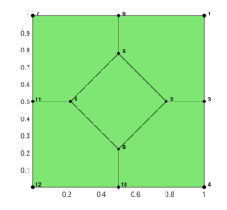
(a) mesh

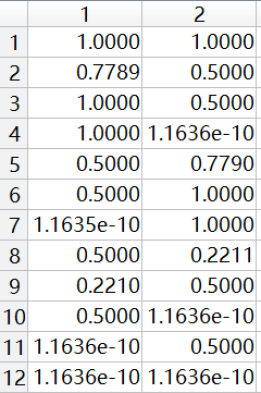
(b) node

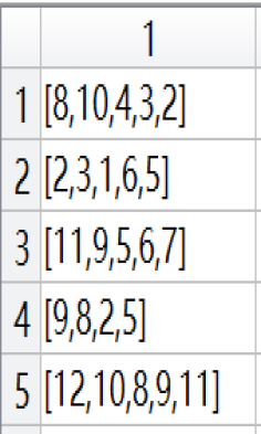
(c) elem

Fig. 1: Example of a polygonal mesh

Using the basic data structures, we can extract the topological or combinatorial structure of a polygonal mesh. These data are referred to as the auxiliary data structures as given in Tab. 1. The combinatorial structure will benefit the implementation of virtual element methods. The idea stems from the treatment of triangulation in $i$FEM for finite element methods [26], which is generalized to polygonal meshes with certain modifications.

Tab. 1: Auxiliary data structures

edge

elem2edge

bdEdge

edge2elem

neighbor

node2elem

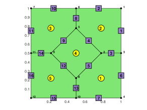
Fig. 2: Illustration of the auxiliary data structures.

edge. The d.o.f.s in (10) and (11) are edge-oriented. In the matrix edge(1:NE,1:2), the first and second rows contain indices of the starting and ending points. The column is sorted in the way that for the $k$-th edge, edge(k,1)<edge(k,2). The indices of these edges are are marked with purple boxes as shown in Fig. 2.

Following [26], we shall use the name convention a2b to represent the link form a to b. This link is usually the map from the local index set to the global index set. Throughout this paper, we use the symbols N, NT, and NE to represent the number of nodes, elements, and edges.

elem2edge. The cell array elem2edge establishes the map of local index of edges in each polygon to its global index in matrix edge. For instance, elem2edge{1} = [13,7,6,3,5] for the mesh in Fig. 2.

bdEdge. This matrix exacts the boundary edges from edge.

edge2elem. The matrix edge(1:NE,1:2) records the neighboring polygons for each edge. In Fig. 2, edge(3,1:2) = [1,2]. For a boundary edge, the outside is specified to the element sharing it as an edge.

neighbor. We use the cell array neighbor to record the neighboring polygons for each element. For example, neighbor{4} = [5,1,2,3], where the $i$-th entry corresponds to the $i$-th edge of the current element. Note that for a boundary edge, the neighboring polygon is specified to the current element, for instance, neighbor{1} = [5,1,1,2,4].

node2elem. This cell array finds the elements sharing a common nodes. For example, node2elem{2} = [1,2,4].

In addition, we provide a subroutine auxgeometry.m to compute some useful geometric quantities, such as the barycenter centroid, the diameter diameter and the area area of each element.

2.2.3 Computation of the elliptic projection

Transition matrix

The shape functions of $V_{k}(K)$ are written in the following compact notation

$$\boldsymbol{\phi}^{T}=(\boldsymbol{\phi}_{1},\boldsymbol{\phi}_{2},\cdots,\boldsymbol{\phi}_{N_{k}}),$$

where $N_{k}=2N_{v}+1$ is the cardinality of the local basis set. The basis of $\widehat{V}_{k}(K)$ is given by

$$\boldsymbol{\widehat{\boldsymbol{m}}}^{T}=(\boldsymbol{\widehat{\boldsymbol{m}}}_{1},\boldsymbol{\widehat{\boldsymbol{m}}}_{2},\cdots,\boldsymbol{\widehat{\boldsymbol{m}}}_{\widehat{N}_{p}}).$$

Noting that $\widehat{V}_{k}(K)\subset V_{k}(K)$, we set $\boldsymbol{\widehat{\boldsymbol{m}}}^{T}=\boldsymbol{\phi}^{T}\boldsymbol{D}$, where $\boldsymbol{D}$ is referred to as the transition matrix from the elliptic projection space $\widehat{V}_{k}(K)$ to the virtual element space $V_{k}(K)$. By the definition of the d.o.f.s,

$$\widehat{\boldsymbol{m}}_{\alpha}=\sum\limits_{i=1}^{N_{k}}\boldsymbol{\phi}_{i}\boldsymbol{D}_{i\alpha},\quad\boldsymbol{D}_{i\alpha}=\chi_{i}(\widehat{\boldsymbol{m}}_{\alpha}).$$

For every $\boldsymbol{v}\in\widehat{V}_{k}(K)$, by definition, $\boldsymbol{v}\in\mathbb{K}\nabla\mathbb{P}_{k+1}(K)$. For $k=1$, the scaled monomials of $\mathbb{P}_{k+1}(K)=\mathbb{P}_{2}(K)$ are

$$m^{T}=(m_{1},m_{2},\cdots,m_{N_{m}}),\quad N_{m}=6,$$

with

$$m_{1}(x,y)=1,~{}~{}m_{2}(x,y)=\frac{x-x_{K}}{h_{K}},~{}~{}m_{3}(x,y)=\frac{y-y_{K}}{h_{K}},$$

$$m_{4}(x,y)=\frac{(x-x_{K})^{2}}{h_{K}^{2}},~{}~{}m_{5}(x,y)=\frac{(x-x_{K})(y-y_{K})}{{h_{K}^{2}}},~{}~{}m_{6}(x,y)=\frac{(y-y_{K})^{2}}{h_{K}^{2}},$$

where $(x_{K},y_{K})$ and $h_{K}$ are the barycenter and diameter of $K$, respectively. We then choose

$$\widehat{\boldsymbol{m}}_{\alpha}=\mathbb{K}\nabla(h_{K}m_{\alpha+1}),\quad\alpha=1,\cdots,\widehat{N}_{m}=N_{m}-1=5,$$ (18)

with the explicit expressions given by

$$\widehat{\boldsymbol{m}}_{1}=\mathbb{K}\begin{bmatrix}1\\ 0\end{bmatrix},\quad\widehat{\boldsymbol{m}}_{2}=\mathbb{K}\begin{bmatrix}0\\ 1\end{bmatrix},\quad\widehat{\boldsymbol{m}}_{3}=\mathbb{K}\begin{bmatrix}2m_{2}\\ 0\end{bmatrix},\quad\widehat{\boldsymbol{m}}_{4}=\mathbb{K}\begin{bmatrix}m_{3}\\ m_{2}\end{bmatrix},\quad\widehat{\boldsymbol{m}}_{5}=\mathbb{K}\begin{bmatrix}0\\ 2m_{3}\end{bmatrix}.$$

We now compute the transition matrix. For $\chi_{i}$ with $i=1,\cdots,N_{v}$ in (10), noting that $\boldsymbol{v}\cdot\boldsymbol{n}|_{e}\in\mathbb{P}_{1}(e)$, the trapezoidal rule gives

$$\chi_{i}(\boldsymbol{v})=\int_{e_{i}}(\boldsymbol{v}\cdot\boldsymbol{n}){\rm d}s=\frac{1}{2}(\boldsymbol{v}(z_{i})+\boldsymbol{v}(z_{i+1}))\cdot(h_{e_{i}}\boldsymbol{n}_{e_{i}}),\quad\boldsymbol{v}=\widehat{\boldsymbol{m}}_{\alpha}.$$ (19)

For $\chi_{N_{v}+i}$ with $i=1,\cdots,N_{v}$ in (11), using the Simpson formula yields

$$\chi_{N_{v}+i}(\boldsymbol{v}) =\int_{e_{i}}(\boldsymbol{v}\cdot\boldsymbol{n})\frac{s-s_{e_{i}}}{h_{e_{i}}}{\rm d}s=\frac{h_{e_{i}}}{6}(f(z_{i})+4f(s_{e_{i}})+f(z_{i+1}))$$

$$=\frac{h_{e_{i}}}{6}(f(z_{i})+f(z_{i+1})),\quad f=(\boldsymbol{v}\cdot\boldsymbol{n})\frac{s-s_{e_{i}}}{h_{e_{i}}}$$

$$=\frac{1}{6}\Big{(}\boldsymbol{v}(z_{i})\cdot\boldsymbol{n}_{e_{i}}(s_{i}-s_{e_{i}})+\boldsymbol{v}(z_{i+1})\cdot\boldsymbol{n}_{e_{i}}(s_{i+1}-s_{e_{i}})\Big{)}$$

$$=\frac{1}{6}\Big{(}\boldsymbol{v}(z_{i})\cdot\boldsymbol{n}_{e_{i}}\frac{-1}{2}h_{e_{i}}+\boldsymbol{v}(z_{i+1})\cdot\boldsymbol{n}_{e_{i}}\frac{1}{2}h_{e_{i}}\Big{)}$$

$$=\frac{1}{12}\Big{(}\boldsymbol{v}(z_{i+1})-\boldsymbol{v}(z_{i})\Big{)}\cdot(\boldsymbol{n}_{e_{i}}h_{e_{i}}),\quad\boldsymbol{v}=\widehat{\boldsymbol{m}}_{\alpha}.$$ (20)

For $\chi_{2N_{v}+1}$ in (12), the integration by parts gives

$$\chi_{2N_{v}+1}(\boldsymbol{v}) =\int_{K}{\rm rot}\boldsymbol{v}{\rm d}x=\int_{K}(\partial_{1}v_{2}-\partial_{2}v_{1}){\rm d}x$$

$$=\int_{\partial K}(v_{2}n_{1}-v_{1}n_{2}){\rm d}s=\int_{\partial K}(\boldsymbol{v}\cdot\boldsymbol{t}){\rm d}s$$

$$=\sum\limits_{i=1}^{N_{v}}\frac{1}{2}(\boldsymbol{v}(z_{i})+\boldsymbol{v}(z_{i+1}))\cdot(h_{e_{i}}\boldsymbol{t}_{e_{i}}),\quad\boldsymbol{v}=\widehat{\boldsymbol{m}}_{\alpha}.$$

According to the above discussion, the transition matrix is calculated as follows.

⬇

1K = pde.K; % coefficient matrix

2 % ------- element information ----------

3 index = elem{iel}; Nv = length(index);

4 xK = centroid(iel,1); yK = centroid(iel,2); hK = diameter(iel);

5 x = node(index,1); y = node(index,2);

6 v1 = 1:Nv; v2 = [2:Nv,1]; % loop index for vertices or edges

7 xe = (x(v1)+x(v2))/2; ye = (y(v1)+y(v2))/2; % mid-edge points

8 Ne = [y(v2)-y(v1), x(v1)-x(v2)]; % he*ne

9 Te = [-Ne(:,2), Ne(:,1)]; % he*te

10

11 % ------- scaled monomials --------

12 m2 = @(x,y) (x-xK)./hK;

13 m3 = @(x,y) (y-yK)./hK;

14 m4 = @(x,y) (x-xK).^2./hK^2;

15 m5 = @(x,y) (x-xK).*(y-yK)./hK^2;

16 m6 = @(x,y) (y-yK).^2./hK^2;

17 % \hat{m}_a = K*grad(hK*m_{a+1})

18 mh1 = @(x,y) [K(1,1)+0*x; K(2,1)+0*x];

19 mh2 = @(x,y) [K(1,2)+0*x; K(2,2)+0*x];

20 mh3 = @(x,y) [2*K(1,1)*m2(x,y); 2*K(2,1)*m2(x,y)];

21 mh4 = @(x,y) [K(1,1)*m3(x,y)+K(1,2)*m2(x,y); K(2,1)*m3(x,y)+K(2,2)*m2(x,y)];

22 mh5 = @(x,y) [2*K(1,2)*m3(x,y); 2*K(2,2)*m3(x,y)];

23 mh = @(x,y) [mh1(x,y), mh2(x,y), mh3(x,y), mh4(x,y), mh5(x,y)];

24

25 % -------- transition matrix ----------

26 NdofA = 2*Nv+1; Nmh = 5;

27 D = zeros(NdofA,Nmh);

28 for i = 1:Nv % loop of edges

29 % v at z_i, z_{i+1} for v = [mK1,...,mK5]

30 va = mh(x(v1(i)),y(v1(i))); vb = mh(x(v2(i)),y(v2(i)));

31 % chi_i, i = 1,...,Nv

32 D(i,:) = 1/2*Ne(i,:)*(va+vb);

33 % chi_{Nv+i}, i = 1,...,Nv

34 D(Nv+i,:) = 1/12*Ne(i,:)*(vb-va);

35 % chi_{2Nv+1}

36 D(end,:) = D(end,:) + 1/2*Te(i,:)*(va+vb);

37 end

Here, K is for $\mathbb{K}$ and mhat is for $\boldsymbol{\widehat{\boldsymbol{m}}}^{T}$.

Elliptic projection matrices

We denote the matrix representation of the $\widehat{\Pi}^{K}$-projection by $\boldsymbol{\widehat{\Pi}}^{K}$ in the sense that

$$\widehat{\Pi}^{K}(\boldsymbol{\phi}_{1},\boldsymbol{\phi}_{2},\cdots,\boldsymbol{\phi}_{N_{k}})=(\boldsymbol{\phi}_{1},\boldsymbol{\phi}_{2},\cdots,\boldsymbol{\phi}_{N_{k}})\boldsymbol{\widehat{\Pi}}^{K}\quad\mbox{or}\quad\widehat{\Pi}^{K}\boldsymbol{\phi}^{T}=\boldsymbol{\phi}^{T}\boldsymbol{\widehat{\Pi}}^{K}.$$

By the definition of d.o.f.s, the $j$-th column of $\boldsymbol{\widehat{\Pi}}^{K}$ is the d.o.f vector of $\widehat{\Pi}^{K}\boldsymbol{\phi}_{j}$, i.e., $\boldsymbol{\widehat{\Pi}}^{K}=\Big{(}\chi_{i}(\widehat{\Pi}^{K}\boldsymbol{\phi}_{j})\Big{)}$. The elliptic projection vector $\widehat{\Pi}^{K}\boldsymbol{\phi}^{T}$ can be expanded in the basis $\boldsymbol{\widehat{\boldsymbol{m}}}^{T}$ of the elliptic projection space $\widehat{V}_{k}(K)$ as $\widehat{\Pi}^{K}\boldsymbol{\phi}^{T}=\widehat{\boldsymbol{m}}^{T}\boldsymbol{\widehat{\Pi}}_{*}^{K}$. It is easy to check that $\boldsymbol{\widehat{\Pi}}^{K}=\boldsymbol{D}\boldsymbol{\widehat{\Pi}}_{*}^{K}$.

The definition 8 is equivalent to

$$a^{K}(\widehat{\boldsymbol{m}},\widehat{\Pi}^{K}\boldsymbol{\phi}^{T})=a^{K}(\widehat{\boldsymbol{m}},\boldsymbol{\phi}^{T})\quad\mbox{or}\quad\widehat{\boldsymbol{G}}\boldsymbol{\widehat{\Pi}}_{*}^{K}=\widehat{\boldsymbol{B}},$$

where

$$\widehat{\boldsymbol{G}}=a^{K}(\widehat{\boldsymbol{m}},\widehat{\boldsymbol{m}}^{T}),\quad\widehat{\boldsymbol{B}}=a^{K}(\widehat{\boldsymbol{m}},\boldsymbol{\phi}^{T}).$$

We also have the consistency relation $\widehat{\boldsymbol{G}}=\widehat{\boldsymbol{B}}\boldsymbol{D}$.

We now compute $\widehat{\boldsymbol{B}}$. From (9) and (18), one has

$$\widehat{\boldsymbol{B}}_{\alpha i} =a^{K}(\widehat{\boldsymbol{m}}_{\alpha},\boldsymbol{\phi}_{i})=-h_{K}\int_{K}m_{\alpha+1}{\rm div}\boldsymbol{\phi}_{i}{\rm d}x+h_{K}\int_{\partial K}m_{\alpha+1}\boldsymbol{\phi}_{i}\cdot\boldsymbol{n}{\rm d}s$$

$$=:-h_{K}I_{1}(\alpha,i)+h_{K}I_{2}(\alpha,i),$$

where

$$I_{1}(\alpha,i)=\int_{K}m_{\alpha+1}{\rm div}\boldsymbol{\phi}_{i}{\rm d}x,\quad I_{2}(\alpha,i)=\int_{\partial K}m_{\alpha+1}\boldsymbol{\phi}_{i}\cdot\boldsymbol{n}{\rm d}s.$$

For $I_{1}$, noting that ${\rm div}\boldsymbol{\phi}_{i}$ is constant when $k=1$, set ${\rm div}\boldsymbol{\phi}_{i}=c_{i}m_{1}=c_{i}$, which gives

$$c_{i}=|K|^{-1}\int_{K}{\rm div}\boldsymbol{\phi}_{i}{\rm d}x=|K|^{-1}\int_{\partial K}\boldsymbol{\phi}_{i}\cdot\boldsymbol{n}{\rm d}s=\begin{cases}|K|^{-1},\quad&i=1,\cdots,N_{v},\\ 0,\quad&i>N_{v},\end{cases}$$

and hence

$$I_{1}(\alpha,i)=\int_{K}m_{\alpha+1}{\rm div}\boldsymbol{\phi}_{i}{\rm d}x=c_{i}\int_{K}m_{\alpha+1}{\rm d}x.$$

The first term is now computed in MATLAB as follows.

⬇

1 % first term

2 nodeT = [node(index,:);centroid(iel,:)];

3 elemT = [(Nv+1)*ones(Nv,1),(1:Nv)',[2:Nv,1]'];

4 m = @(x,y) [m2(x,y), m3(x,y), m4(x,y), m5(x,y), m6(x,y)]; % m_{a+1},...

5 ci = zeros(1,NdofA); ci(1:Nv) = 1/area(iel);

6 Intm = integralTri(m,3,nodeT,elemT);

7 I1 = Intm'*ci;

The subroutine integralTri.m calculates the integral on a polygonal element which is triangulated with the basic data structures nodeT and elemT.

For $I_{2}$, since $\boldsymbol{\phi}_{i}\cdot\boldsymbol{n}|_{e_{j}}\in\mathbb{P}_{1}({e_{j}})$ ($i=1,\cdots,2N_{v}+1$), set

$$\boldsymbol{\phi}_{i}\cdot\boldsymbol{n}_{e_{j}}|_{e_{j}}=c_{0}^{i}+c_{1}^{i}\frac{s-s_{e_{j}}}{h_{e_{j}}},$$

where $s$ it the natural parameter of the edge $e_{j}$ and $s_{e_{j}}$ is the mid-point in the local parametrization. Noting that

$$\int_{e}\Big{(}\frac{s-s_{e}}{h_{e}}\Big{)}^{\alpha}\Big{(}\frac{s-s_{e}}{h_{e}}\Big{)}^{\beta}{\rm d}s=\frac{h_{e}}{(\alpha+\beta+1)}\Big{(}\frac{1}{2^{\alpha+\beta+1}}-\frac{1}{(-2)^{\alpha+\beta+1}}\Big{)},$$

we then obtain

$$\begin{cases}h_{e_{j}}c_{0}^{i}=\int_{e_{j}}\boldsymbol{\phi}_{i}\cdot\boldsymbol{n}{\rm d}s=:r_{j}^{i},\\ \frac{1}{12}h_{e_{j}}c_{1}^{i}=\int_{e_{j}}\boldsymbol{\phi}_{i}\cdot\boldsymbol{n}\frac{s-s_{e_{j}}}{h_{e_{j}}}{\rm d}s=:s_{j}^{i}.\end{cases}$$

By definition, the nonzero elements of $r_{j}^{i}$ and $s_{j}^{i}$ are

$$r_{j}^{j}=s_{j}^{j+N_{v}}=1,\quad j=1,\cdots,N_{v}.$$

We have

$$c_{0}^{i}=\frac{1}{h_{e_{j}}}r_{j}^{i},\quad c_{1}^{i}=\frac{12}{h_{e_{j}}}s_{j}^{i},$$

and hence

$$\boldsymbol{r}_{j}^{i}(s):=\boldsymbol{\phi}_{i}\cdot(h_{e_{j}}\boldsymbol{n}_{e_{j}})|_{e_{j}}=r_{j}^{i}+12s_{j}^{i}\frac{s-s_{e_{j}}}{h_{e_{j}}}.$$

It is obvious that

$$\boldsymbol{r}_{j}^{i}(s_{a})=r_{j}^{i}-6s_{j}^{i},\quad\boldsymbol{r}_{j}^{i}(s_{e})=r_{j}^{i},\quad\boldsymbol{r}_{j}^{i}(s_{b})=r_{j}^{i}+6s_{j}^{i},$$

where, $s_{a}$, $s_{e}$ and $s_{b}$ correspond to the starting point, middle point and ending point in the local parameterization, respectively.

Observing that the Simpson formula is accurate for cubic polynomials, we have

$$I_{2}(\alpha,i) =\sum\limits_{j=1}^{N_{v}}\int_{e_{j}}m_{\alpha+1}\boldsymbol{\phi}_{i}\cdot\boldsymbol{n}{\rm d}s$$

$$=\sum\limits_{j=1}^{N_{v}}\frac{h_{e_{j}}}{6}(m_{\alpha+1}\boldsymbol{\phi}_{i}(z_{j})+4m_{\alpha+1}\boldsymbol{\phi}_{i}(z_{e_{j}})+m_{\alpha+1}\boldsymbol{\phi}_{i}(z_{j+1})\cdot\boldsymbol{n}_{e_{j}}$$

$$=\frac{1}{6}\sum\limits_{j=1}^{N_{v}}m_{\alpha+1}(z_{j})\boldsymbol{r}_{j}^{i}(s_{a})+4m_{\alpha+1}(z_{e_{j}})\boldsymbol{r}_{j}^{i}(s_{e})+m_{\alpha+1}(z_{j+1})\boldsymbol{r}_{j}^{i}(s_{b})$$

or

$$I_{2}(\alpha,:)=\frac{1}{6}\sum\limits_{j=1}^{N_{v}}m_{\alpha+1}(z_{j})\boldsymbol{r}_{j}(s_{a})+4m_{\alpha+1}(z_{e_{j}})\boldsymbol{r}_{j}(s_{e})+m_{\alpha+1}(z_{j+1})\boldsymbol{r}_{j}(s_{b}).$$

Then the second term and the matrices $\widehat{\boldsymbol{B}}$ and $\widehat{\boldsymbol{G}}$ can be computed as follows.

⬇

1 % second term

2 rij = zeros(Ndof,Nv); rij(1:Nv,:) = eye(Nv);

3 sij = zeros(Ndof,Nv); sij(Nv+1:2*Nv,:) = eye(Nv);

4 rija = rij- 6*sij;

5 rije = rij;

6 rijb = rij + 6*sij;

7 I2 = zeros(np,Ndof);

8 for j = 1:Nv

9 ma = m(x(v1(j)),y(v1(j)));

10 me = m(xe(j),ye(j));

11 mb = m(x(v2(j)),y(v2(j)));

12 rja = rija(:,j)'; rje = rije(:,j)'; rjb = rijb(:,j)';

13 I2 = I2 + 1/6*(ma'*rja + 4*me'*rje + mb'*rjb);

14 end

15 % \hat{B} and \hat{G}

16 Bs = hK*(-I1+I2); Gs = Bs*D

2.2.4 Computation and assembly of the stiffness matrix and load vector

The stiffness matrix

The local stiffness matrix of $A$ in (16) is $A^{K}=A^{K}_{1}+A^{K}_{2}$, where

$$A^{K}_{1}(i,j) =a^{K}(\widehat{\Pi}^{K}\boldsymbol{\phi}_{j},\widehat{\Pi}^{K}\boldsymbol{\phi}_{i}),$$

$$A^{K}_{2}(i,j) =\|\mathbb{K}^{-1}\|S^{K}(\boldsymbol{\phi}_{j}-\widehat{\Pi}^{K}\boldsymbol{\phi}_{j},\boldsymbol{\phi}_{i}-\widehat{\Pi}^{K}\boldsymbol{\phi}_{i})$$

$$=\|\mathbb{K}^{-1}\|\sum\limits_{i=1}^{N_{k}}\chi_{r}(\boldsymbol{\phi}_{j}-\widehat{\Pi}^{K}\boldsymbol{\phi}_{j})\chi_{r}(\boldsymbol{\phi}_{i}-\widehat{\Pi}^{K}\boldsymbol{\phi}_{i}).$$

The first term is written in matrix form as

$$A_{K}^{1}=a^{K}(\widehat{\Pi}^{K}\boldsymbol{\phi},\widehat{\Pi}^{K}\boldsymbol{\phi}^{T})=(\boldsymbol{\widehat{\Pi}}_{*}^{K})^{T}a^{K}(\widehat{\boldsymbol{m}},\widehat{\boldsymbol{m}}^{T})\boldsymbol{\widehat{\Pi}}_{*}^{K}=(\boldsymbol{\widehat{\Pi}}_{*}^{K})^{T}\widehat{\boldsymbol{G}}\boldsymbol{\widehat{\Pi}}_{*}^{K}.$$

For the second term, from $\chi_{r}(\widehat{\Pi}^{K}\boldsymbol{\phi}_{i})=(\boldsymbol{\widehat{\Pi}}^{K})_{ri}$ one has

$$A_{K}^{2}=\|\mathbb{K}^{-1}\|({\bf{I}}-\boldsymbol{\widehat{\Pi}}^{K})^{T}({\bf{I}}-\boldsymbol{\widehat{\Pi}}^{K}).$$

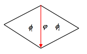
Fig. 3: Illustration of the global and local basis functions

Note that the signs of the d.o.f.s in (10) vary with the edge orientation, which means the global basis function $\boldsymbol{\varphi}_{i}$ restriction to the element may have the opposite sign with the local basis function $\boldsymbol{\phi}_{i}$. As shown in Fig. 3, $e$ is an interior edge with the global orientation given by the arrow. Let $\boldsymbol{\varphi}$ be the global basis function, and let $\boldsymbol{\phi}_{1}$ and $\boldsymbol{\phi}_{2}$ be the local basis functions corresponding to the left and right elements, respectively. Then one has

$$\boldsymbol{\phi}_{1}=-\boldsymbol{\varphi}|_{K_{1}},\quad\boldsymbol{\phi}_{2}=\boldsymbol{\varphi}|_{K_{2}}.$$

Obviously, the sign can be determined by computing the difference between the two indices of the end points of $e$. For this reason, one only needs to compute the elementwise signs of the edges of $\partial K$. The code is given as

⬇

1%% Get elementwise signs of basis functions

2bdEdgeIdx = bdStruct.bdEdgeIdx; E = false(NE,1); E(bdEdgeIdx) = 1;

3sgnBase = cell(NT,1);

4for iel = 1:NT

5 index = elem{iel}; Nv = length(index); NdofA = 2*Nv+1;

6 sgnedge = sign(diff(index([1:Nv,1])));

7 id = elem2edge{iel}; sgnbd = E(id); sgnedge(sgnbd) = 1;

8 sgnelem = ones(NdofA,1); sgnelem(1:Nv) = sgnedge;

9 sgnBase{iel} = sgnelem;

10end

Note that the positive signs of the boundary edges are recovered in the above code.

Since $a^{K}(\pm\boldsymbol{\phi}_{i},\pm\boldsymbol{\phi}_{j})=\pm\cdot\pm a^{K}(\boldsymbol{\phi}_{i},\boldsymbol{\phi}_{j})$, we can introduce a signed stiffness matrix sgnK to add the correct signs to the local stiffness matrix. The matrix $A^{K}$ can be computed in the following way.

⬇

1 % -------- sign matrix and sign vector -------

2 sgnelem = sgnBase{iel};

3 sgnK = sgnelem*sgnelem';

4

5 % ------------- stiffness matrix -------------

6 % Projection

7 Pis = Gs\Bs; Pi = D*Pis; I = eye(size(Pi));

8 % Stiffness matrix A

9 AK = Pis'*Gs*Pis + norm(inv(K),'fro')*(I-Pi)'*(I-Pi); % G = Gs

10 AK = AK.*sgnK;

11 AK = reshape(AK',1,[]); % straighten as row vector for easy assembly

By the definition of $Q_{h}$, on each element $K$, the basis function $\psi_{l}\in\mathbb{P}_{k-1}(K)$. Only one basis $\psi_{l}=m_{1}=1$ for $k=1$. Hence, the element matrix $B^{K}$ of $B$ in (16) is a column vector of size $N_{k}\times 1$ (Note that $B$ is of size ${{\leavevmode\lstinline{{\lst@@@set@language\lst@@@set@numbers\lst@@@set@frame\lst@@@set@rulecolor\lst@@@set@language\lst@@@set@numbers\lst@@@set@frame\lst@@@set@rulecolor\lst@@@set@language\lst@@@set@numbers\lst@@@set@frame\footnotesize\small(2{\@listingGroup{ltx_lst_identifier}{NE}}+{\@listingGroup{ltx_lst_identifier}{NT}})}}}\times\leavevmode\lstinline{{\lst@@@set@language\lst@@@set@numbers\lst@@@set@frame\lst@@@set@rulecolor\lst@@@set@language\lst@@@set@numbers\lst@@@set@frame\lst@@@set@rulecolor\lst@@@set@language\lst@@@set@numbers\lst@@@set@frame\footnotesize\small{\@listingGroup{ltx_lst_identifier}{NT}}}}}$), and

$$B^{K}_{j1} =b^{K}(\boldsymbol{\phi}_{j},m_{1})=\int_{K}m_{1}{\rm div}\boldsymbol{\phi}_{j}{\rm d}x=\int_{K}{\rm div}\boldsymbol{\phi}_{j}{\rm d}x$$

$$=\int_{\partial K}\boldsymbol{\phi}_{j}\cdot\boldsymbol{n}{\rm d}s=\begin{cases}1,\quad&1\leq j\leq N_{v},\\ 0,\quad&j>N_{v}.\end{cases}$$

The sign of each entry is adjusted by using $b^{K}(\pm\boldsymbol{\phi}_{i},\psi_{j})=\pm b^{K}(\boldsymbol{\phi}_{i},\psi_{j})$.

⬇

1 % Stiffness matrix B

2 BK = zeros(NdofA,1); BK(1:Nv) = 1;

3 BK = BK.*sgnelem;

4 BK = reshape(BK',1,[]); % straighten as row vector for easy assembly

For $k=1$, $Q_{h}$ is piecewise constant, and hence has NT basis functions given by

$$\psi_{l}(x)=\begin{cases}1,\quad&x\in K_{l},\\ 0,\quad&\mbox{otherwise}.\end{cases}$$

Obviously, the vector in (15) is

$${d_{l}=\int_{K_{l}}{\rm d}x=|K_{l}|,\quad l=1,\cdots,M=\leavevmode\lstinline{{\lst@@@set@language\lst@@@set@numbers\lst@@@set@frame\lst@@@set@rulecolor\lst@@@set@language\lst@@@set@numbers\lst@@@set@frame\lst@@@set@rulecolor\lst@@@set@language\lst@@@set@numbers\lst@@@set@frame\footnotesize\small{\@listingGroup{ltx_lst_identifier}{NT}}}}}.$$

We compute the elliptic projections and provide the assembly index by looping over the elements. The assembly index for the matrices $A$ and $B$ is given by

⬇

1 % ------ assembly index for bilinear forms --------

2 NdofA = 2*Nv+1; NdofB = 1;

3 indexDofA = [elem2edge{iel},elem2edge{iel}+NE,iel+2*NE];

4 indexDofB = iel;

5 iiA(idA+1:idA+NdofA^2) = reshape(repmat(indexDofA, NdofA,1), [], 1);

6 jjA(idA+1:idA+NdofA^2) = repmat(indexDofA(:), NdofA, 1);

7 ssA(idA+1:idA+NdofA^2) = AK(:);

8 idA = idA + NdofA^2;

9 iiB(idB+1:idB+NdofA*NdofB) = reshape(repmat(indexDofA, NdofB,1), [], 1);

10 jjB(idB+1:idB+NdofA*NdofB) = repmat(indexDofB(:), NdofA, 1);

11 ssB(idB+1:idB+NdofA*NdofB) = BK(:);

12 idB = idB + NdofA*NdofB;

Afterwards, we can assemble the matrices $A$ and $B$ using the MATLAB functions sparse.

⬇

1A = sparse(iiA,jjA,ssA,NNdofA,NNdofA);

2B = sparse(iiB,jjB,ssB,NNdofA,NNdofB);

3d = area; % for Lagrange multiplier

The load vector

For the right-hand side, in view of (16), we only need to compute $\boldsymbol{f}=(-(f,\psi_{l}))$. For $k=1$, the local vector is

$$\boldsymbol{f}_{K}=-(f,\psi_{l})_{K}=-\int_{K}f{\rm d}x,$$

with the realization reading

⬇

1 % -------- load vector f ----------

2 fxy = @(x,y) pde.f([x,y]); % f(p) = f([x,y])

3 rhs = integralTri(fxy,3,nodeT,elemT); rhs = rhs';

4 fK = -rhs;

The assembly index for the vector $\boldsymbol{f}$ is given by

⬇

1 % ------- assembly index for rhs -------

2 elemb(ib+1:ib+NdofB) = indexDofB(:);

3 Fb(ib+1:ib+NdofB) = fK(:);

4 ib = ib + NdofB;

Then $\boldsymbol{f}$ can be assembled using the MATLAB functions accumarray.

⬇

1 FB = accumarray(elemb,ffB,[NNdofB 1]);

To sum up, the linear system without boundary conditions imposed is given by

⬇

1%% Get block linear system

2kk = sparse(NNdof+1,NNdof+1); ff = zeros(NNdof+1,1);

3kk(1:NNdofA,1:NNdofA) = A;

4kk(1:NNdofA, (1:NNdofB)+NNdofA) = B;

5kk((1:NNdofB)+NNdofA, 1:NNdofA) = B';

6kk((1:NNdofB)+NNdofA, end) = d;

7kk(end, (1:NNdofB)+NNdofA) = d';

8ff((1:NNdofB)+NNdofA) = FB;

Note that the extra variable $\lambda$ leads to NNdof+1 rows or columns.

2.2.5 Applying the boundary conditions

The boundary condition $\boldsymbol{u}\cdot\boldsymbol{n}=g$ is now viewed as a Dirichlet condition for $\boldsymbol{u}$, which provides the values of the first two types of d.o.f.s, i.e.,

$$\chi_{i}(\boldsymbol{u})=\int_{e_{i}}(\boldsymbol{u}\cdot\boldsymbol{n}){\rm d}s,\quad i=1,\cdots,N_{v},$$

$$\chi_{N_{v}+i}(\boldsymbol{u})=\int_{e_{i}}(\boldsymbol{u}\cdot\boldsymbol{n})\frac{s-s_{e_{i}}}{h_{e_{i}}}{\rm d}s,\quad i=1,\cdots,N_{v}$$

The Simpson rule is used to approximate the exact ones as follows.

⬇

1%% Apply Dirichlet boundary conditions

2% bdDof, freeDof

3bdEdge = bdStruct.bdEdge; bdEdgeIdx = bdStruct.bdEdgeIdx;

4id = [bdEdgeIdx; bdEdgeIdx+NE];

5isBdDof = false(NNdof+1,1); isBdDof(id) = true;

6bdDof = (isBdDof); freeDof = ($\neg$isBdDof);

7% bdval

8u = pde.uexact;

9z1 = node(bdEdge(:,1),:); z2 = node(bdEdge(:,2),:); ze = (z1+z2)./2;

10e = z1-z2; % e = z2-z1

11Ne = [-e(:,2),e(:,1)];

12chi1 = 1/6*sum((u(z1)+4*u(ze)+u(z2)).*Ne,2); % u*n = g

13chi2 = 1/12*sum((u(z2)-u(z1)).*Ne,2);

14bdval = [chi1;chi2];

15% sol

16sol = zeros(NNdof+1,1);

17sol(bdDof) = bdval;

18ff = ff - kk*sol;

19

20%% Set solver

21sol(freeDof) = kk(freeDof,freeDof)\ff(freeDof);

22uh = sol(1:NNdofA); % u = [u1,u2]

23ph = sol(NNdofA+1:end-1);

24

25%% Store information for computing errors

26info.Ph = Ph; info.elem2dof = elem2dof;

27info.kk = kk; %info.freeDof = freeDof;

To compute the discrete errors, one can store the matrix representation $\boldsymbol{\widehat{\Pi}}_{*}^{K}$ and the assembly index elem2dof in the function file.

2.2.6 Numerical example

In this paper, all examples are implemented in MATLAB R2019b. Our code is available from GitHub (https://github.com/Terenceyuyue/mVEM). The subroutine Darcy_mixedVEM.m is used to compute the numerical solutions and the test script main_Darcy_mixedVEM.m verifies the convergence rates. The PDE data is generated by Darcydata.m.

Example 2.1.

Let $\mathbb{K}$ be the identity matrix. The right-hand side $f$ and the boundary conditions are chosen in such a way that the exact solution of (1) is $p(x,y)=\sin(\pi x)\cos(\pi y)$.

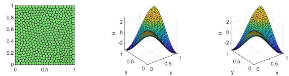
Fig. 4: Numerical and exact results for the Darcy problem

To test the accuracy of the proposed method we consider a sequence of polygonal meshes, which is a Centroidal Voronoi Tessellation of the unit square in 32, 64, 128, 256 and 512 polygons. These meshes are generated by the MATLAB toolbox - PolyMesher introduced in [45]. we report the nodal values of the exact solution and the piecewise elliptic projection $\widehat{\Pi}^{K}\boldsymbol{u}_{h}$ in Fig. 4. The convergence orders of the errors against the mesh size $h$ are shown in Fig. 5. Generally speaking, $h$ is proportional to $N^{-1/2}$, where $N$ is the total number of elements in the mesh. The convergence rate with respect to $h$ is estimated by assuming $\text{ErrL2}(h)=ch^{\alpha}$, and by computing a least squares fit to this log-linear relation. As observed from Fig. 5, the convergence rate of $p$ is linear with respect to the $L^{2}$ norm, and the VEM ensures the quadratic convergence for $\boldsymbol{u}$ in the $L^{2}$ norm, which is consistent with the theoretical prediction in [8].

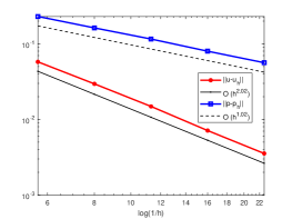
Fig. 5: The convergence rates for the Darcy problem

2.2.7 A lifting mixed virtual element method

We can obtain the second-order convergence of the variable $p$ using the lifting technique. To do so, we modify the original virtual element space to the following lifting space

$$V_{k}(K) =\{\boldsymbol{v}\in H({\rm div};K)\cap H({\rm rot};K):\boldsymbol{v}\cdot\boldsymbol{n}|_{e}\in\mathbb{P}_{k}(e),$$

$$\hskip 85.35826pt{\rm div}\boldsymbol{v}|_{K}\in\mathbb{P}_{k}(K),~{}~{}{\rm rot}\boldsymbol{v}|_{K}\in\mathbb{P}_{k-1}(K)\},$$

with the d.o.f.s given by

$$\int_{e}\boldsymbol{v}\cdot\boldsymbol{n}q{\rm d}s,\quad q\in\mathbb{M}_{k}(e),~{}~{}e\subset\partial K,$$

$$\int_{K}\boldsymbol{v}\cdot\nabla q{\rm d}x,\quad q\in\mathbb{M}_{k}(K)\backslash\{1\},$$

$$\int_{K}{\rm rot}\boldsymbol{v}q{\rm d}x,\quad q\in\mathbb{M}_{k-1}(K).$$

In the lowest order case $k=1$, the local d.o.f.s are arranged as

$$\chi_{i}(\boldsymbol{v})=\int_{e_{i}}(\boldsymbol{v}\cdot\boldsymbol{n}){\rm d}s,\quad i=1,\cdots,N_{v},$$

$$\chi_{N_{v}+i}(\boldsymbol{v})=\int_{e_{i}}(\boldsymbol{v}\cdot\boldsymbol{n})\frac{s-s_{e_{i}}}{h_{e_{i}}}{\rm d}s,\quad i=1,\cdots,N_{v},$$

$$\chi_{2N_{v}+1}(\boldsymbol{v})=\int_{K}\boldsymbol{v}\cdot\nabla m_{2}{\rm d}x=\frac{1}{h_{K}}\int_{K}\boldsymbol{v}_{1}{\rm d}x,$$

$$\chi_{2N_{v}+2}(\boldsymbol{v})=\int_{K}\boldsymbol{v}\cdot\nabla m_{3}{\rm d}x=\frac{1}{h_{K}}\int_{K}\boldsymbol{v}_{2}{\rm d}x,$$

$$\chi_{2N_{v}+3}(\boldsymbol{v})=\int_{K}{\rm rot}\boldsymbol{v}{\rm d}x.$$

In this case, $Q_{h}$ will be replaced by the piecewise linear space.

We repeat the test in Example 2.1. The subroutine Darcy_LiftingmixedVEM.m is used to compute the numerical solutions and the test script main_Darcy_LiftingmixedVEM.m verifies the convergence rates. The exact and numerical solutions for the variable $p$ are shown in Fig. 6. The corresponding convergence rates are displayed in Fig. 7, from which we observe the second-order convergence for both variables.

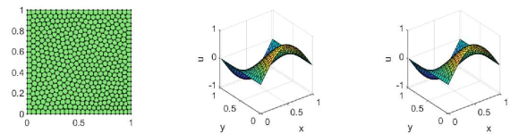
Fig. 6: $p_{h}$ and $p$ for the lifting VEM of the Darcy problem

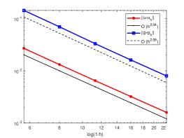
Fig. 7: The convergence rates for the lifting VEM of the Darcy problem

3 Polygonal mesh generation and refinement

The polygonal meshes can be generated by using the MATLAB toolbox - PolyMesher introduced in [45]. We provide a modified version in our package and give a very detailed description in the document. The test script is meshfun.m and we present a mesh for a complex geometry in Fig. 8.

Fig. 8: A polygonal mesh generated by PolyMesher for a complex geometry.

We present some basic functions to show the polygonal meshes, including marking of the nodes, elements and (boundary) edges, see showmesh.m, findnode.m, findelem.m and findedge.m. For the convenience of the computation, some auxiliary mesh data are introduced (see Subsection 2.2.2). The idea stems from the treatment of triangulation in $i$FEM, which is generalized to polygonal meshes with certain modifications. We also provide a boundary setting function to identify the Neumann and Dirichlet boundaries (See setboundary.m).

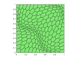
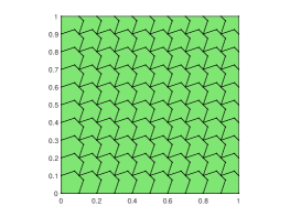
Fig. 9: A distorted mesh and a non-convex octagonal mesh.

The routine distortionmesh.m is used to generate a distorted mesh. Let $(\xi,\eta)$ be the coordinates on the original mesh. The nodes of the distorted mesh are obtained by the following transformation

$$x=\xi+t_{c}\sin(2\pi\xi)\sin(2\pi\eta),\quad y=\eta+t_{c}\sin(2\pi\xi)\sin(2\pi\eta),$$

where $(x,y)$ is the coordinate of new nodal points; $t_{c}$, taken as $0.1$ in the computation, is the distortion parameter. Such an example is displayed in Fig. 9(a). In the literature of VEMs (see [25] for example), one often finds the test for the non-convex mesh in Fig. 9(b), which is generated by nonConvexMesh.m in our package.

The polygonal meshes can also be obtained from a Delaunay triangulation by establishing its dual mesh. The implementation is given in dualMesh.m. Several examples are given in main_dualMesh.m as shown in Fig. 10.

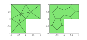
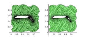
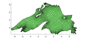
Fig. 10: Dual meshes generated by dualMesh.m.

Due to the large flexibility of the meshes, researchers have focused on the a posterior error analysis of the VEMs and made some progress in recent years [18, 24, 20, 29, 19]. We present an efficient implementation of the mesh refinement for polygonal meshes [52] (see PolyMeshRefine.m). To the best of our knowledge, this is the first publicly available implementation of the polygonal mesh refinement algorithms. We divide elements by connecting the midpoint of each edge to its barycenter, which may be the most natural partition frequently used in VEM papers. To remove small edges, some additional neighboring polygons of the marked elements are included in the refinement set by requiring the one-hanging-node rule: limit the mesh to have just one hanging node per edge. The current implementation requires that the barycenter of each element is an interior point.

4 Poisson equation

In this section we focus on the virtual element methods for the reaction-diffusion problem

$$\begin{cases}-\Delta u+\alpha u=f\quad&\mbox{in}~{}~{}\Omega,\\ u=0\quad&\mbox{on}~{}~{}\partial\Omega,\end{cases}$$ (21)

where $\alpha$ is a nonnegative constant and $\Omega$ is a polygonal domain.

4.1 Conforming VEMs

Consider the first virtual element space [7]

$$V_{k}(K):=\left\{v\in H^{1}(K):\Delta v\in\mathbb{P}_{k-2}(K)~{}~{}{\rm in}~{}~{}K,\quad v|_{\partial K}\in\mathbb{B}_{k}(\partial K)\right\},$$ (22)

where

$$\mathbb{B}_{k}(\partial K):=\left\{v\in C(\partial K):v|_{e}\in\mathbb{P}_{k}(e),~{}~{}e\subset\partial K\right\}.$$

Equipped with the d.o.f.s in [7], a computable approximate bilinear form can be constructed by using the elliptic projector $\Pi_{k}^{\nabla}$. To ensure the accuracy and the well-posedness of the discrete method, a natural candidate to approximate the reaction term $(u,v)_{K}$ in the local bilinear form is $(\Pi_{k}^{0}u,\Pi_{k}^{0}v)_{K}$, where $\Pi_{k}^{0}$ is the $L^{2}$ projection onto $\mathbb{P}_{k}(K)$ and $(\cdot,\cdot)_{K}$ the usual $L^{2}(K)$ inner product. Nevertheless, $\Pi_{k}^{0}$ can not be computed in terms of d.o.f.s attached to $V_{k}(K)$. Therefore, Ahmad et al. [2] modified the VEM space (22) to a local enhancement space

$$W_{k}(K)=\left\{w\in\widetilde{V}_{k}(K):(w-\Pi_{k}^{\nabla}w,q)_{K}=0,~{}~{}q\in\mathbb{M}_{k}(K)\backslash\mathbb{M}_{k-2}(K)\right\},$$ (23)

where the lifting space is

$$\widetilde{V}_{k}(K):=\left\{v\in H^{1}(K):v|_{\partial K}\in\mathbb{B}_{k}(\partial K),~{}~{}\Delta v\in\mathbb{P}_{k}(K)~{}~{}\mbox{in}~{}K\right\}.$$

In this space, the operator $\Pi_{k}^{0}$ can be easily computed using $\Pi_{k}^{\nabla}$ and the local d.o.f.s related to $W_{k}(K)$:

• $\chi_{a}$: the values at the vertices of $K$,

  $$\chi_{i}(v)=v(a_{i}),\quad a_{i}\mbox{ is a vertex of }K.$$

• $\chi_{e}^{k-2}$: the moments on edges up to degree $k-2$,

  $$\chi_{e}(v)=|e|^{-1}(m_{e},v)_{e},\quad m_{e}\in\mathbb{M}_{k-2}(e),~{}~{}e\subset\partial K.$$

• $\chi_{K}^{k-2}$: the moments on element $K$ up to degree $k-2$,

  $$\chi_{K}(v)=|K|^{-1}(m_{K},v)_{K},\quad m_{K}\in\mathbb{M}_{k-2}(K).$$

In what follows, denote by $W_{k,h}$ a finite dimensional subspace of $V$, produced by combining all $W_{k}(K)$ for $K\in\mathcal{T}_{h}$ in a standard way. We define a local $H^{1}$-elliptic projection operator $\Pi_{k}^{\nabla}:{H^{1}}(K)\to\mathbb{P}_{k}(K)$ by the relations

$$(\nabla\Pi_{k}^{\nabla}v,\nabla p)_{K}=(\nabla v,\nabla p)_{K},\quad p\in\mathbb{P}_{k}(K).$$ (24)

Since $(\nabla\cdot,\nabla\cdot)$ is only semi-positive definite, the constraints

$$\int_{\partial K}v{\rm d}s=\int_{\partial K}\Pi_{1}^{\nabla}v{\rm d}s,\quad k=1;\qquad\int_{K}v{\rm d}x=\int_{K}\Pi_{k}^{\nabla}v{\rm d}x,\quad k\geq 2$$

should be imposed. The VEM is to find $u_{h}\in W_{k,h}$ such that

$${a_{h}^{c}}(u_{h},v_{h})=\langle f_{h},v_{h}\rangle,\quad v_{h}\in W_{k,h},$$ (25)

where

$${a_{h}^{c}}(u_{h},v_{h}):=\sum\limits_{K\in\mathcal{T}_{h}}{a_{h}^{c,K}(u_{h},v_{h})}$$

and $\langle\cdot,\cdot\rangle$ is the duality pairing between $W_{k,h}^{\prime}$ and $W_{k,h}$. The local approximate bilinear form is

$$a_{h}^{c,K}(v,w)=a^{K}(\Pi_{k}^{\nabla}v,\Pi_{k}^{\nabla}w)+\alpha(\Pi_{k}^{0}v,\Pi_{k}^{0}w)_{K}+S^{K}(v-\Pi_{k}^{\nabla}v,w-\Pi_{k}^{\nabla}w)$$

where $a^{K}(v,w)=(\nabla v,\nabla w)_{K}$ and the stabilization term is realized as

$$S^{K}(v-\Pi_{k}^{\nabla}v,w-\Pi_{k}^{\nabla}w):=(1+\alpha h_{K}^{2})\boldsymbol{\chi}(v-\Pi_{k}^{\nabla}v)\cdot\boldsymbol{\chi}(w-\Pi_{k}^{\nabla}w),$$

where $\boldsymbol{\chi}$ is referred to as the d.o.f vector of a VEM function on $K$.

Let $\phi^{T}=(\phi_{1},\phi_{2},\cdots,\phi_{N_{k}})$ be the basis of $W_{k}(K)$ and let $m^{T}=(m_{1},m_{2},\cdots,m_{N_{m}})$ be the scaled monomials. Then the transition matrix $D$ can be defined through $m^{T}=\phi^{T}D$. The matrix expressions of $\Pi_{k}^{\nabla}\phi^{T}$ in the basis $\phi^{T}$ and $m^{T}$ are defined by

$$\Pi_{k}^{\nabla}\phi^{T}=\phi^{T}\boldsymbol{\Pi}_{k}^{\nabla},\quad\Pi_{k}^{\nabla}\phi^{T}=m^{T}\boldsymbol{\Pi}_{k*}^{\nabla}.$$

One easily finds that $\boldsymbol{\Pi}_{k}^{\nabla}=D\boldsymbol{\Pi}_{k*}^{\nabla}$. In vector form, the definition of (24) can be rewritten as

$$\begin{cases}a^{K}(m,\Pi_{k}^{\nabla}\phi^{T})=a^{K}(m,\phi^{T}),\\ P_{0}(\Pi_{k}^{\nabla}\phi^{T})=P_{0}(\phi^{T}),\end{cases}$$

where

$$P_{0}(v)=\int_{\partial K}v{\rm d}s,\quad k=1;\qquad P_{0}(v)=\int_{K}v{\rm d}x,\quad k\geq 2.$$

Define

$$G=a^{K}(m,m^{T}),\quad B=a^{K}(m,\phi^{T}).$$ (26)

Then

$$\begin{cases}G\boldsymbol{\Pi}_{k*}^{\nabla}=B,\\ P_{0}(m^{T})\boldsymbol{\Pi}_{k*}^{\nabla}=P_{0}(\phi^{T})\end{cases}\quad\mbox{or}\quad\tilde{G}\boldsymbol{\Pi}_{k*}^{\nabla}=\tilde{B}.$$

Note that one always has the consistency relations $G=BD$ and $\tilde{G}=\tilde{B}D$.

We remark that in the implementation of the VEM, the most involved step is to compute the boundary part of $B$ resulted from the integration by parts:

$$B=\int_{K}\nabla m\cdot\nabla\phi^{T}\mathrm{d}x=-\int_{K}\Delta m\cdot\phi^{T}\mathrm{d}x+\sum\limits_{e\subset\partial K}\int_{e}(\nabla m\cdot{{\boldsymbol{n}}_{e}})\phi^{T}\mathrm{d}s.$$ (27)

For the conforming VEMs, however, we can compute the second term of (27) by using the assembling technique for finite element methods since the VEM function restriction to the boundary $\partial K$ is piecewise polynomial. For example, the computation for $k=2$ reads

⬇

1% second term

2I2 = zeros(Nm, Ndof);

3v1 = 1:Nv; v2 = [2:Nv,1];

4elem1 = [v1(:), v2(:), v1(:)+Nv];

5for im = 1:Nm

6 gradmc = Gradmc{im};

7 F1 = 1/6*sum(gradmc(x(v1), y(v1)).*Ne, 2);

8 F2 = 1/6*sum(gradmc(x(v2), y(v2)).*Ne, 2);

9 F3 = 4/6*sum(gradmc(xe, ye).*Ne, 2);

10 F = [F1, F2, F3];

11 I2(im, :) = accumarray(elem1(:), F(:), [Ndof 1]);

12end

Example 4.1.

Let $\alpha=1$ and $\Omega=(0,1)^{2}$. The Neumann boundary condition is imposed on $x=0$ and $x=1$ with the exact solution given by $u(x,y)=\sin(2x+0.5)\cos(y+0.3)+\log(1+xy)$.

The test script is main_PoissonVEMk3.m for $k=3$. The optimal rate of convergence of the $H^{1}$-norm (3rd order), $L^{2}$-norm (4th order) and energy norm (3rd order) is observed for $k=3$ from Fig. 11.

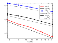
(a) $k=1$

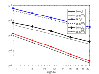
(b) $k=2$

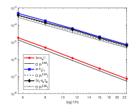
(c) $k=3$

Fig. 11: Convergence rates for Example 4.1.

Example 4.2.

In this example, the exact solution is $u(x,y)=y^{2}\sin(\pi x)$. The domain $\Omega$ is taken as a unit disk.

The Neumann boundary condition is imposed on the boundary of the upper semicircle. The nodal values are displayed in Fig. 12.

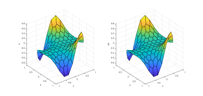
Fig. 12: Numerical and exact solutions for Example 4.2 ($k=1$)

4.2 Nonconforming VEMs

4.2.1 The standard treatment of the domain boundary

Now we consider the nonconforming VEMs proposed in [6] for the problem (21) with $\alpha=0$. The local nonconforming virtual element space is defined by

$$V_{k}^{nc}(K)=\left\{v\in H^{1}(K):\Delta v\in\mathbb{P}_{k-2}(K),~{}~{}\partial_{\boldsymbol{n}}v|_{e}\in\mathbb{P}_{k-1}(e),~{}e\subset\partial K\right\},\quad k\geq 1,$$

and the d.o.f.s can be chosen as

• $\boldsymbol{\chi}_{\partial K}(v)$: the moments on edges up to degree $k-1$,

  $$\chi_{e}(v)=|e|^{-1}(m_{e},v)_{e},\quad m_{e}\in\mathbb{M}_{k-1}(e),~{}~{}e\subset\partial K.$$

• $\boldsymbol{\chi}_{K}(v)$: the moments on $K$ up to degree $k-2$,

  $$\chi_{K}(v)=|K|^{-1}(m_{K},v)_{K},\quad m_{K}\in\mathbb{M}_{k-2}(K).$$

The elliptic projection and the discrete problem can be constructed in the same way as before. We briefly discuss the implementation of $k=1$. In this case, the first term for the matrix $B$ in (27) vanishes and the second term is obtained from the Kronecher’s property $\chi_{i}(\phi_{j})=\sigma_{ij}$, which is realized as follows.

⬇

1% B

2B = zeros(Nm,Nv);

3for i = 1:Nv % loop of edges

4 gi = sum(Gradm.*repmat(Ne(i,:),3,1), 2); % gradm*Ne

5 B(:,i) = gi;

6end

For completeness, we also present the application of the Neumann boundary conditions. Let $e$ be a boundary edge of the Neumann boundary $\Gamma_{N}$. Then the local boundary term is approximated as

$$F_{e}=\int_{e}\Pi_{0,e}^{0}g_{N}\phi_{e}\mathrm{d}s,$$

where $g_{N}=\partial_{\boldsymbol{n}}u=\nabla u\cdot\boldsymbol{n}_{e}$, $\Pi_{0,e}^{0}$ is the $L^{2}$ projection on $e$, and $\phi_{e}$ is the local basis function associated with the d.o.f $\chi_{e}(v)=|e|^{-1}(m_{e},v)_{e}$. For problems with known explicit solutions, we provide the gradient $g_{N}=\nabla u$ in the PDE data instead and compute the true $g_{N}$ in the M-file. Obviously, the $L^{2}$ projection $\Pi_{0,e}^{0}g_{N}$ can be computed by the mid-point formula or the trapezoidal rule. The computation reads

⬇

1%% Assemble Neumann boundary conditions

2bdEdgeN = bdStruct.bdEdgeN; bdEdgeIdxN = bdStruct.bdEdgeIdxN;

3if $\neg$isempty(bdEdgeN)

4 g_N = pde.Du;

5 z1 = node(bdEdgeN(:,1),:); z2 = node(bdEdgeN(:,2),:);

6 e = z1-z2; % e = z2-z1

7 Ne = [-e(:,2),e(:,1)]; % scaled ne

8 F1 = sum(Ne.*g_N(z1),2);

9 F2 = sum(Ne.*g_N(z2),2);

10 FN = (F1+F2)/2;

11 ff = ff + accumarray(bdEdgeIdxN(:), FN(:),[NNdof 1]);

12end

Note that the structure data bdStruct stores all necessary information of boundary edges, which is obtained by using the subroutine setboundary.m. In the above code, bdEdgeN gives the data structure bdEdge in Subsection 2.2.2 for Neumann edges and bdEdgeIdxN provides their indices in the data structure edge.

We still consider Example 4.1 and display the convergence rates in the discrete $L^{2}$ and $H^{1}$ norms in Fig. 13. The optimal rate of convergence is observed for both norms and the test script is main_PoissonVEM_NC.m.

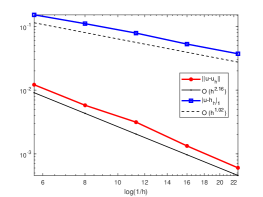
Fig. 13: Convergence rates of the Poisson equation for the nonconforming VEM ($k=1$)

4.2.2 A continuous treatment of the domain boundary

In some cases it may be not convenient to deal with the moments on the domain boundary $\partial\Omega$. To do so, we can modify the corresponding local virtual element spaces to the following one

$$V_{k}^{ncb}(K) =\Big{\{}v\in H^{1}(K):\Delta v\in\mathbb{P}_{k-2}(K),~{}~{}\partial_{\boldsymbol{n}}v|_{e}\in\mathbb{P}_{k-1}(e),~{}~{}e~{}\mbox{is an interior edge}$$

$$\hskip 85.35826ptv|_{e}\in\mathbb{P}_{k}(e),~{}~{}e~{}\mbox{ is a boudary edge},\quad e\subset\partial K\Big{\}}.$$

We repeat the test in Fig. 13 and the discrete $L^{2}$ and $H^{1}$ errors are listed in Tab. 2. Please refer to main_PoissonVEM_NCb.m for the test script.

Tab. 2: The discrete errors for the modified nonconforming VEM

$\sharp{\rm Dof}$	$h$	ErrL2	ErrH1
97	1.768e-01	1.17632e-02	1.51836e-01
193	1.250e-01	5.37635e-03	1.10077e-01
383	8.839e-02	3.14973e-03	7.82566e-02
760	6.250e-02	1.43956e-03	5.26535e-02
1522	4.419e-02	6.48454e-04	3.71405e-02

5 Linear elasticity problems

The linear elasticity problem is

$$\begin{cases}-{\rm div}\boldsymbol{\sigma}=\boldsymbol{f}\quad&\text{in}~{}~{}~{}\Omega,\\ \boldsymbol{u}={\boldsymbol{0}}\quad&\text{on}~{}~{}~{}\Gamma_{0},\\ \boldsymbol{\sigma n}=\boldsymbol{g}\quad&\text{on}~{}~{}~{}\Gamma_{1},\end{cases}$$ (28)

where $\boldsymbol{n}=(n_{1},n_{2})^{T}$ denotes the outer unit vector normal to $\partial\Omega$. The constitutive relation for linear elasticity is

$$\boldsymbol{\sigma}(\boldsymbol{u})=2\mu\boldsymbol{\varepsilon}(\boldsymbol{u})+\lambda({\rm div}\boldsymbol{u})\boldsymbol{I},$$

where $\boldsymbol{\sigma}=(\sigma_{ij})$ and $\boldsymbol{\varepsilon}=(\varepsilon_{ij})$ are the second order stress and strain tensors, respectively, satisfying $\varepsilon_{ij}=\frac{1}{2}(\partial_{i}u_{j}+\partial_{j}u_{i})$, $\lambda$ and $\mu$ are the Lamé constants, $\boldsymbol{I}$ is the identity matrix, and ${\rm div}\boldsymbol{u}=\partial_{1}u_{1}+\partial_{2}u_{2}$.

5.1 Conforming VEMs

5.1.1 The displacement type

The equilibrium equation in (28) can also be written in the form

$$-\mu\Delta\boldsymbol{u}-(\lambda+\mu){\text{grad}}({\rm div}\boldsymbol{u})=\boldsymbol{f}\quad{\text{in}}~{}~{}\Omega,$$ (29)

which is referred to as the displacement type or the Navier type in what follows. In this case, we only consider $\Gamma_{0}=\Gamma:=\partial\Omega$. The first term $\Delta\boldsymbol{u}$ can be treated as the vector case of the Poisson equation, which is clearly observed in the implementation.

The continuous variational problem is to find $\boldsymbol{u}\in\boldsymbol{V}:=\boldsymbol{H}_{0}^{1}(\Omega)$ such that

$$a(\boldsymbol{u},\boldsymbol{v})=(\boldsymbol{f},\boldsymbol{v}),\quad\boldsymbol{v}\in\boldsymbol{V},$$

where the bilinear form restriction to $K$ is

$$a^{K}(\boldsymbol{u},\boldsymbol{v}) =\mu\int_{K}{\nabla\boldsymbol{u}\cdot\nabla{\boldsymbol{v}}}\mathrm{d}x+(\lambda+\mu)\int_{K}({\rm div}\boldsymbol{u})({\rm div}{\boldsymbol{v}})\mathrm{d}x$$

$$=:\mu a_{\nabla}^{K}(\boldsymbol{u},{\boldsymbol{v}})+(\lambda+\mu)a_{{\rm div}}^{K}(\boldsymbol{u},{\boldsymbol{v}})$$

with

$$a_{\nabla}^{K}(\boldsymbol{u},{\boldsymbol{v}})=\int_{K}{\nabla\boldsymbol{u}\cdot\nabla{\boldsymbol{v}}}\mathrm{d}x,\quad a_{{\rm div}}^{K}(\boldsymbol{u},{\boldsymbol{v}})=\int_{K}({\rm div}\boldsymbol{u})({\rm div}{\boldsymbol{v}})\mathrm{d}x.$$

The local virtual element space $\boldsymbol{V}_{k}(K)$ can be simply taken as the tensor-product of $V_{k}(K)$ defined in (22), i.e., $\boldsymbol{V}_{k}(K)=(V_{k}(K))^{2}$. Let $\Pi^{\nabla}:\boldsymbol{V}_{k}(K)\to(\mathbb{P}_{k}(K))^{2}$ be the elliptic projector induced by $a_{\nabla}^{K}$. Then the approximate bilinear form can be split as

$$a_{h}^{K}(\boldsymbol{u},{\boldsymbol{v}})=\mu a_{h,\nabla}^{K}(\boldsymbol{u},{\boldsymbol{v}})+(\lambda+\mu)a_{h,{\rm div}}^{K}(\boldsymbol{u},{\boldsymbol{v}}),$$

where

$$a_{h,\nabla}^{K}(\boldsymbol{u},{\boldsymbol{v}})=a_{\nabla}^{K}({\Pi^{\nabla}}\boldsymbol{u},{\Pi^{\nabla}}{\boldsymbol{v}})+S^{K}(\boldsymbol{u}-\Pi^{\nabla}\boldsymbol{u},\boldsymbol{v}-\Pi^{\nabla}\boldsymbol{v}),$$

$$a_{h,{\rm div}}^{K}(\boldsymbol{u},{\boldsymbol{v}})=(\Pi_{k-1}^{0}{\rm div}\boldsymbol{u},\Pi_{k-1}^{0}{\rm div}\boldsymbol{v})_{K},$$

and the stabilization term for $k=1$ is given by

$$S^{K}(\boldsymbol{u},{\boldsymbol{v}})=\sum\limits_{i=1}^{N_{v}}\chi_{i}(\boldsymbol{u})\cdot\chi_{i}(\boldsymbol{v}),\quad\chi_{i}(\boldsymbol{u})=[\chi_{i}(u_{1}),\chi_{i}(u_{2})]^{T}.$$

The discrete problem is: Find $\boldsymbol{u}_{h}\in\boldsymbol{V}_{h}$ such that

$$a_{h}(\boldsymbol{u}_{h},\,\boldsymbol{v}_{h})=\langle\boldsymbol{f}_{h},\,\boldsymbol{v}_{h}\rangle,\quad\boldsymbol{v}_{h}\in\boldsymbol{V}_{h},$$ (30)

where

$$a_{h}(\boldsymbol{u}_{h},\,\boldsymbol{v}_{h})=\sum\limits_{K\in\mathcal{T}_{h}}a_{h}^{K}(\boldsymbol{u}_{h},{\boldsymbol{v}}_{h})$$

and the approximation of the right hand side is given by [54]

$$\langle\boldsymbol{f}_{h},\boldsymbol{v}_{h}\rangle=(\boldsymbol{f},P_{h}\boldsymbol{v}_{h}),$$ (31)

where

$$P_{h}\boldsymbol{v}_{h}|_{K}=\frac{1}{|\partial K|}\int_{\partial K}\boldsymbol{v}_{h}{\rm d}s.$$

Let $\phi_{1},\cdots,\phi_{N}$ be the basis functions of the scalar space $V_{k}(K)$. Then the basis functions of the vector space $\boldsymbol{V}_{k}(K)$ can be defined by

$${\overline{\phi}_{1}},\cdots,{\overline{\phi}_{N}},{\underline{\phi}_{1}},\cdots,{\underline{\phi}_{N}},$$

where

$${\overline{\phi}_{i}}=\begin{bmatrix}\phi_{i}\\ 0\end{bmatrix},\qquad{\underline{\phi}_{i}}=\begin{bmatrix}0\\ \phi_{i}\end{bmatrix},\quad i=1,\cdots,N.$$

Similarly, we introduce the notation

$${\overline{m}_{\alpha}}=\begin{bmatrix}m_{\alpha}\\ 0\end{bmatrix},\qquad{\underline{m}_{\alpha}}=\begin{bmatrix}0\\ m_{\alpha}\end{bmatrix},\quad\alpha=1,\cdots,N_{m}.$$ (32)

These vector functions will be written in a compact form as

$$\boldsymbol{m}^{T}=[{\overline{m}_{1}},\cdots,{\overline{m}_{N_{m}}},{\underline{m}_{1}},\cdots,{\underline{m}_{N_{m}}}]=:[\overline{m}^{T},\underline{m}^{T}],$$

$$\boldsymbol{\phi}^{T}=[{\overline{\phi}_{1}},\cdots,{\overline{\phi}_{N_{k}}},{\underline{\phi}_{1}},\cdots,{\underline{\phi}_{N_{k}}}]=:[\overline{\phi}^{T},\underline{\phi}^{T}].$$

We introduce the transition matrix $\boldsymbol{D}$ such that $\boldsymbol{m}^{T}={\boldsymbol{\phi}^{T}}{\boldsymbol{D}}$. One easily finds that $\boldsymbol{D}={\rm diag}(D,D)$, where $D$ is the transition matrix for the scalar case, i.e., $m^{T}=\phi^{T}D$. This block structure is also valid for the elliptic projection matrices. That is,

$$\boldsymbol{G}={\rm diag}(G,G),\quad\boldsymbol{B}={\rm diag}(B,B),\quad\boldsymbol{G}=\boldsymbol{B}\boldsymbol{D},$$

where $G$ and $B$ are the same ones given in (26).

In the following, we consider the matrix expression of the $L^{2}$ projector $\Pi_{k-1}^{0}{\rm div}$ satisfying

$$\int_{K}{\Pi_{k-1}^{0}({\rm div}{\boldsymbol{v}})p}\mathrm{d}x=\int_{K}{({\rm div}{\boldsymbol{v}})p}\mathrm{d}x,~{}~{}p\in{\mathbb{P}_{k-1}}(K).$$

The vector form can be written as

$$\int_{K}{{m^{0}}\Pi_{k-1}^{0}({\rm div}{\boldsymbol{\phi}^{T}})}\mathrm{d}x=\int_{K}{{m^{0}}({\rm div}{\boldsymbol{\phi}^{T}})}\mathrm{d}x,$$

where $m^{0}$ is the vector consisting of the scaled monomials of order $\leq k-1$. Let $\boldsymbol{\Pi}_{0*}$ be the matrix expression of $\Pi_{k-1}^{0}({\rm div}{\boldsymbol{\phi}^{T}})$ in the basis $(m^{0})^{T}$, i.e.,

$$\Pi_{k-1}^{0}({\rm div}{\boldsymbol{\phi}^{T}})=(m^{0})^{T}\boldsymbol{\Pi}_{0*}.$$

Then $H_{0}\boldsymbol{\Pi}_{0*}=C_{0}$, where

$$H_{0}=\int_{K}{{m^{0}}{{({m^{0}})}^{T}}}\mathrm{d}x,\quad~{}C_{0}=\int_{K}{{m^{0}}({\rm div}{\boldsymbol{\phi}^{T}})}\mathrm{d}x.$$

For $k=1$, one has $m^{0}=m_{1}=1$ and

$$C_{0}=\int_{K}{{m^{0}}({\rm div}{\boldsymbol{\phi}^{T}})}\mathrm{d}x=\int_{K}{{\rm div}{\boldsymbol{\phi}^{T}}}\mathrm{d}x=\int_{\partial K}{{\boldsymbol{\phi}^{T}}\cdot{\boldsymbol{n}}}\mathrm{d}s,$$

where

$$\int_{\partial K}{{\boldsymbol{\phi}^{T}}\cdot{\boldsymbol{n}}}\mathrm{d}s=\int_{\partial K}{[\overline{\phi}^{T}\cdot{\boldsymbol{n}},\underline{\phi}^{T}\cdot{\boldsymbol{n}}]}\mathrm{d}s=\int_{\partial K}{[\phi^{T}\cdot{n_{x}},\phi^{T}\cdot{n_{y}}]}\mathrm{d}s.$$ (33)

We remark that (33) can be assembled along the boundary $\partial K$ using the technique in finite element methods.

⬇

1v1 = 1:Nv; v2 = [2:Nv,1];

2H0 = area(iel);

3C0 = zeros(1,2*Nv);

4F = 1/2*[(1*Ne); (1*Ne)]; % [he*n1, he*n2]

5C0(:) = accumarray([elem1(:);elem1(:)+Nv], F(:), [2*Nv 1]);

Example 5.1.

We consider a typical example to check the locking-free property of the proposed method. The right-hand side $\boldsymbol{f}$ and the boundary conditions are chosen in such a way that the exact solution is

$$\boldsymbol{u}(x,y)=\begin{bmatrix}(-1+\cos 2\pi x)\sin 2\pi y\\ -(-1+\cos 2\pi y)\sin 2\pi x\end{bmatrix}+\frac{1}{1+\lambda}\sin\pi x\sin\pi y\begin{bmatrix}1\\ 1\end{bmatrix}.$$

One easily finds that the proposed VEM is exactly the $\mathbb{P}_{1}$-Lagrange element when the polygonal mesh degenerates into a triangulation, in which case the method cannot get a uniform convergence with respect to the Lamé constant $\lambda$. However, for general polygonal meshes, the method seems to be robust with respect to $\lambda$ (see Fig. 14), and the optimal rates of convergence are achieved in the nearly incompressible case as shown in Fig. 15, although we have not justified it in a theoretical way or found a counter example. Please refer to main_elasticityVEM_Navier.m for the test script.

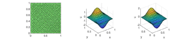
Fig. 14: The exact and numerical nodal values for the linear elasticity problem of displacement type with $\lambda=10^{8}$ and $\mu=1$.

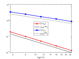
Fig. 15: The performance of the VEM for the linear elasticity problem of displacement type with $\lambda=10^{8}$ and $\mu=1$.

5.1.2 The tensor type

Let $\boldsymbol{f}\in\boldsymbol{L}^{2}(\Omega)$. For simplicity, we still consider $\Gamma_{0}=\partial\Omega$. The tensor-type variational formulation of (28) is to find $\boldsymbol{u}\in\boldsymbol{V}$ such that

$$a(\boldsymbol{u},\boldsymbol{v})=(\boldsymbol{f},\boldsymbol{v}),\quad\boldsymbol{v}\in\boldsymbol{V},$$ (34)

where

$$a(\boldsymbol{u},\boldsymbol{v})=2\mu(\boldsymbol{\varepsilon}(\boldsymbol{u}),\boldsymbol{\varepsilon}(\boldsymbol{v}))+\lambda({\rm div}\boldsymbol{u},{\rm div}\boldsymbol{v}),$$ (35)

and

$$(\boldsymbol{f},\boldsymbol{v})=\int_{\Omega}\boldsymbol{f}\boldsymbol{v}\mathrm{d}x.$$

For the ease of the presentation, we introduce the following notation

$$a_{\mu}(\boldsymbol{u},\boldsymbol{v})=(\boldsymbol{\varepsilon}(\boldsymbol{u}),\boldsymbol{\varepsilon}(\boldsymbol{v})),\qquad a_{\lambda}(\boldsymbol{u},\boldsymbol{v})=({\rm div}\boldsymbol{u},{\rm div}\boldsymbol{v}).$$

The conforming VEM for (34) is proposed in [10], where a locking-free analysis is carried out for the virtual element spaces of order $k\geq 2$. The order requirement is to ensure the so-called discrete inf-sup condition and the optimal convergence.

Introduce the elliptic projection

$${\Pi^{a}}:~{}{{\boldsymbol{V}}_{k}}(K)\to{(\mathbb{P}_{k}(K))^{2}},\quad{\boldsymbol{v}}\mapsto{\Pi^{a}}{\boldsymbol{v}},$$

satisfying

$$a_{\mu}^{K}({\Pi^{a}}{\boldsymbol{v}},\boldsymbol{p})=a_{\mu}^{K}({\boldsymbol{v}},\boldsymbol{p}),\quad\boldsymbol{p}\in{(\mathbb{P}_{k}(K))^{2}}.$$ (36)

Note that $\Pi^{a}\boldsymbol{v}$ is unique up to an additive vector in

$$K_{0}:=RM={\rm span}\left\{\begin{bmatrix}1\\ 0\end{bmatrix},~{}~{}\begin{bmatrix}0\\ 1\end{bmatrix},~{}~{}\begin{bmatrix}-y\\ x\end{bmatrix}\right\}.$$

For this reason, we can impose one of the following constraints:

• $$\sum\limits_{i=1}^{N_{v}}(\Pi^{a}\boldsymbol{v}(z_{i}),\boldsymbol{p}(z_{i}))=\sum\limits_{i=1}^{N_{v}}(\boldsymbol{v}(z_{i}),\boldsymbol{p}(z_{i})),~{}~{}\boldsymbol{p}\in K_{0},$$ (37)

• $$\int_{\partial K}(\Pi^{a}\boldsymbol{v})\cdot\boldsymbol{p}\mathrm{d}s=\int_{\partial K}\boldsymbol{v}\cdot\boldsymbol{p}\mathrm{d}s,~{}~{}\boldsymbol{p}\in K_{0}.$$ (38)

• $$\int_{K}{\rm rot}~{}\Pi_{K}^{1}\boldsymbol{v}\mathrm{d}x =\int_{K}{\rm rot}\boldsymbol{v}\mathrm{d}x,$$

  $$\int_{\partial K}\Pi_{K}^{1}\boldsymbol{v}\mathrm{d}s =\int_{\partial K}\boldsymbol{v}\mathrm{d}s,$$ (39)

  where ${\rm rot}\boldsymbol{v}=\nabla\times\boldsymbol{v}=\partial_{1}v_{2}-\partial_{2}v_{1}$. An integration by parts gives

  $$\int_{K}{\rm rot}\boldsymbol{v}{\rm d}x=\int_{\partial K}\boldsymbol{v}\cdot\boldsymbol{t}_{K}{\rm d}s,$$

  where $\boldsymbol{t}_{K}=(-n_{2},n_{1})^{T}$ is the anti-clockwise tangential along $\partial K$.

It is evident that all the three choices can be computed by using the given d.o.f.s.

The discrete problem is the same as the one in (30) with the local approximate bilinear form replaced by

$$a_{h}^{K}(\boldsymbol{v},\boldsymbol{w})=2\mu a_{\mu,h}^{K}(\boldsymbol{v},\boldsymbol{w})+\lambda a_{\lambda,h}^{K}(\boldsymbol{v},\boldsymbol{w}),$$

where

$$a_{\mu,h}^{K}(\boldsymbol{v},\boldsymbol{w})=a_{\mu}^{K}(\Pi^{a}\boldsymbol{v},\Pi^{a}\boldsymbol{w})+S^{K}(\boldsymbol{v}-\Pi^{a}\boldsymbol{v},\boldsymbol{w}-\Pi^{a}\boldsymbol{w}),$$

$$a_{\lambda,h}^{K}(\boldsymbol{v},\boldsymbol{w})=(\Pi_{k-1}^{0}{\rm div}\boldsymbol{v},\Pi_{k-1}^{0}{\rm div}\boldsymbol{w})_{K}.$$

For the lowest-order case $k=1$, an integration by parts gives

$$\boldsymbol{B} =a_{\mu}^{K}(\boldsymbol{m},\boldsymbol{\phi}^{T})=\int_{\partial K}(\boldsymbol{\varepsilon}(\boldsymbol{m})\cdot{\boldsymbol{n}})\cdot{\boldsymbol{\phi}^{T}}\mathrm{d}s$$ (40)

$$=\Big{[}\varepsilon_{11}(\boldsymbol{m})\int_{\partial K}\phi^{T}n_{x}\mathrm{d}s+\varepsilon_{12}(\boldsymbol{m})\int_{\partial K}\phi^{T}n_{y}\mathrm{d}s,$$

$$\hskip 56.9055pt\varepsilon_{21}(\boldsymbol{m})\int_{\partial K}\phi^{T}n_{x}\mathrm{d}s+\varepsilon_{22}(\boldsymbol{m})\int_{\partial K}\phi^{T}n_{y}\mathrm{d}s\Big{]}$$

with

$$\varepsilon_{11}(\boldsymbol{m})=[0,\frac{1}{h_{K}},0,0,0,0]^{T},\qquad\varepsilon_{22}(\boldsymbol{m})=[0,0,0,0,0,\frac{1}{h_{K}}]^{T},$$

$$\varepsilon_{12}(\boldsymbol{m})=\varepsilon_{21}(\boldsymbol{m})=[0,0,\frac{1}{2h_{K}},0,\frac{1}{2h_{K}},0]^{T}.$$

Using the assembling technique for FEMs, the computation of $\boldsymbol{B}$ in MATLAB reads

⬇

1elem1 = [v1(:), v2(:)];

2C0 = zeros(1,2*Nv);

3F = 1/2*[(1*Ne); (1*Ne)]; % [he*n1, he*n2]

4C0(:) = accumarray([elem1(:);elem1(:)+Nv], F(:), [2*Nv 1]);

5E = zeros(6,4);

6E(2,1) = 1/hK; E([3,5],[2,3]) = 1/(2*hK); E(6,4) = 1/hK;

7B = [E(:,1)*C01x+E(:,2)*C01y, E(:,3)*C01x+E(:,4)*C01y];

Note that for the tensor type, we can consider the pure traction problem, i.e., $\Gamma_{1}=\partial\Omega$. The numerical results are similar to that of the VEM of displacement type. The test script is main_elasticityVEM.m. It is worth pointing out that we proposed in [38] a novel conforming locking-free method with a rigorous proof, where several benchmarks are tested and the test script can be found in main_elasticityVEM_reducedIntegration.m.

5.2 Nonconforming VEMs

Nonconforming VEMs for the linear elasticity problems are first introduced in [54] for the pure displacement/traction formulation in two or three dimensions. The proposed method is robust with respect to the Lamé constant for $k\geq 2$.

For $k=1$, one easily finds that

$$\int_{\partial K}\phi^{T}n_{x}{\rm d}s=[h_{e_{1}}n_{1,x},\cdots,h_{e_{N_{v}}}n_{N_{v},x}],$$

where $h_{e_{i}}$ is the length of the edge $e_{i}$ and $\boldsymbol{n}_{e_{i}}=(n_{i,x},n_{i,y})^{T}$. In this case, the computation of $\boldsymbol{B}$ in (40) for the tensor type reads

⬇

1C01x = Ne(:,1)'; C01y = Ne(:,2)';

2B = [E(:,1)*C01x+E(:,2)*C01y, E(:,3)*C01x+E(:,4)*C01y];

We provide the implementation of the displacement type and tensor type in the original nonconforming spaces with the results displayed in Fig. 16(a)(b). Similar to the Poisson equation, we also present the realization of the tensor type in the modified nonconforming spaces and the convergence rate is shown in Fig. 16(c). Here, we still consider the test in Example 5.1 with $\lambda=10^{10}$ and $\mu=1$. As again observed in Fig. 16, the optimal rates of convergence are obtained for all the three methods with general polygonal meshes applied in the nearly incompressible case although we cannot justify it or provide a counter example.

The test scripts are main_elasticityVEM_NavierNC.m, main_elasticityVEM_NC.m and
main_elasticityVEM_NCb.m, respectively.

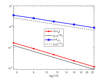
(a) Displacement type

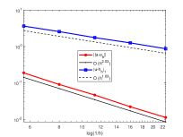
(b) Tensor type

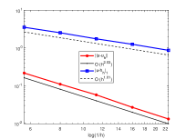
(c) Tensor type with the continuous treatment

Fig. 16: Convergence rates of the nonconforming VEMs for the linear elasticity.

5.3 Several locking-free VEMs

The authors in [41] present two kinds of lowest-order VEMs with consistent convergence, in which the first one is achieved by introducing a special stabilization term to ensure the discrete Korn’s inequality, and the second one can be seen as an extension of the idea of Kouhia and Stenberg suggested in [40] to the virtual element method. We provide the implementation of the second method in elasticityVEM_KouhiaStenberg.m. In this approach, the local space is taken as

$$\boldsymbol{V}(K)=V_{1}^{nc}(K)\times V_{1}(K),$$

where $V_{1}^{nc}(K)$ and $V_{1}(K)$ are the lowest-order nonconforming and conforming virtual element spaces, respectively. In this case, the computation for $k=1$ reads

⬇

1C01xe = Ne(:,1)'; C01ye = Ne(:,2)';

2C01xv = 0.5*(Ne(p1,1)+Ne(p2,1))';

3C01yv = 0.5*(Ne(p1,2)+Ne(p2,2))';

4B = [E(:,1)*C01xe+E(:,2)*C01ye, E(:,3)*C01xv+E(:,4)*C01yv];

We also develop a lowest-order nonconforming virtual element method for planar linear elasticity in [53], which can be viewed as an extension of the idea in [32] to the virtual element method, with the family of polygonal meshes satisfying a very general geometric assumption. The method is shown to be uniformly convergent for the nearly incompressible case with optimal rates of convergence. In addition, we provide a unified locking-free scheme both for the conforming and nonconforming VEMs in the lowest order case. The implementation and the numerical test can be found in [53]. The test scripts are main_elasticityVEM_NCreducedIntegration.m and main_elasticityVEM_NCUniformReducedIntegration.m, respectively.

6 Plate bending problems

In this section we focus on the plate bending problem in the form of

$$\begin{cases}-\partial_{ij}M_{ij}(w)=f\quad&\mbox{in}~{}~{}\Omega\subset\mathbb{R}^{2},\\ w=\partial_{\boldsymbol{n}}w=0\quad&\mbox{on}~{}~{}\partial\Omega,\end{cases}$$

where

$$M_{ij}=D\left((1-\nu)K_{ij}+\nu K_{kk}\delta_{ij}\right),~{}~{}~{}i,j=1,2,~{}~{}k\in\{1,2\},$$

$$K_{ij}=-\partial_{ij}w,~{}~{}~{}i,j=1,2,\quad D=\frac{Et^{3}}{12(1-\nu^{2})}.$$

Note that we have used the summation convention whereby summation is implied when an index is repeated exactly two times. Please refer to [33, 23, 30] for details. The variational problem is to find $w\in V:=H_{0}^{2}(\Omega)$ such that

$$a(w,v)=\ell(v),\quad v\in V,$$

where

$$a(w,v)=\int_{\Omega}M_{ij}(w)K_{ij}(v)\mathrm{d}x,\qquad\ell(v)=\int_{\Omega}fv\mathrm{d}x.$$

6.1 $C^{1}$-continuous VEMs

We first recall the $H^{2}$-conforming virtual element space $V_{k}^{2,c}(K)$ introduced in [23, 30]. For $k\geq 3$, define

$${V_{k}^{2,c}}(K)=\{v\in H^{2}(K):\Delta^{2}v\in\mathbb{P}_{k-4}(K),~{}v|_{e}\in\mathbb{P}_{k}(e),~{}\partial_{\boldsymbol{n}}v|_{e}\in{\mathbb{P}_{k-1}}(e),~{}e\subset\partial K\},$$

while for the lowest order $k=2$, the space is modified as

$$V_{2}^{2,c}(K)=\Big{\{}v\in H^{2}(K):\Delta^{2}v=0,~{}v|_{e}\in\mathbb{P}_{3}(e),~{}\partial_{\boldsymbol{n}}v|_{e}\in\mathbb{P}_{1}(e),~{}e\subset\partial K\Big{\}}.$$

The d.o.f.s are:

• The values of $v(z)$ at the vertices of $K$.

• The values of $h_{z}\partial_{1}v(z)$ and $h_{z}\partial_{2}v(z)$ at the vertices of $K$, where $h_{z}$ is a characteristic length attached to each vertex $z$, for instance, the average of the diameters of the elements having $z$ as a vertex.

• The moments of $v$ on edges up to degree $k-4$,

  $$\chi_{e}(v)=|e|^{-1}(m_{e},v)_{e},\quad m_{e}\in\mathbb{M}_{k-4}(e).$$

• The moments of $\partial_{\boldsymbol{n}}v$ on edges up to degree $k-3$,

  $$\chi_{n_{e}}(v)=(m_{e},\partial_{\boldsymbol{n}}v)_{e},\quad m_{e}\in\mathbb{M}_{k-3}(e).$$

• The moments on element $K$ up to degree $k-4$,

  $$\chi_{K}(v)=|K|^{-1}(m_{K},v)_{K},\quad m_{K}\in\mathbb{M}_{k-4}(K).$$

The elliptic projection can be defined in vector form as

$$\begin{cases}a^{K}(m,\Pi^{K}\phi^{T})=a^{K}(m,\phi^{T}),\\ P_{0}^{1}(\Pi^{K}\phi^{T})=P_{0}^{1}(\phi^{T}),\\ P_{0}^{2}(\nabla\Pi^{K}\phi^{T})=P_{0}^{2}(\nabla\phi^{T}),\end{cases}$$ (41)

where

$$P_{0}^{1}(v)=\frac{1}{N_{v}}\sum\limits_{i=1}^{N_{v}}v(a_{i}),\quad P_{0}^{2}(v)=\int_{\partial K}v\mathrm{d}s.$$

Introduce the following notation

$$Q_{3i}=M_{ij,j},~{}~{}Q_{3\boldsymbol{n}}=Q_{3i}n_{i},\quad M_{\boldsymbol{nn}}=M_{ij}n_{i}n_{j},~{}~{}M_{\boldsymbol{tn}}=M_{ij}t_{i}n_{j},$$

with $\boldsymbol{n}=(n_{1},n_{2})^{T}$ and $\boldsymbol{t}=(-n_{2},n_{1})^{T}$. We then have the integration by parts formula

$$a^{K}(p,v) =-\int_{K}Q_{3i,i}(p)v\mathrm{d}x$$

$$\quad+\int_{\partial K}\left(Q_{3\boldsymbol{n}}(p)+\partial_{\boldsymbol{t}}M_{\boldsymbol{tn}}(p)\right)v\mathrm{d}s-\int_{\partial K}M_{\boldsymbol{nn}}(p)\partial_{\boldsymbol{n}}v\mathrm{d}s$$

$$\quad+\sum\limits_{i=1}^{N_{v}}[M_{\boldsymbol{tn}}(p)](z_{i})v(z_{i}),$$

which implies the computability of the elliptic projection $\Pi^{K}v$ for any $v\in V_{k}^{2,c}(K)$, where the last term is a jump at $z_{i}$ along the boundary $\partial K$, i.e.,

$$[M_{\boldsymbol{tn}}(p)](z_{i})=M_{\boldsymbol{tn}}(p)\Big{|}_{z_{i}^{-}}^{z_{i}^{+}}.$$

We now consider the computation of the elliptic projection matrices. In the lowest order case, the d.o.f.s are

• The values of $v$ at the vertices of $K$,

  $$\chi_{a}(v)=v(z_{i}),\quad i=1,\cdots,N_{v}.$$

• The values of $\nabla v$ at the vertices of $K$,

  $$\chi_{a1}(v)=\partial_{x}v(z_{i}),~{}~{}\chi_{a2}(v)=\partial_{y}v(z_{i}),\quad i=1,\cdots,N_{v}.$$

In the implementation, they are arranged as

$$\chi_{i}(v)=v(z_{i}),\quad i=1,\cdots,N_{v},$$

$$\chi_{N_{v}+i}(v)=h_{\xi}\partial_{x}v(z_{i}),\quad i=1,\cdots,N_{v},$$

$$\chi_{2N_{v}+i}(v)=h_{\xi}\partial_{y}v(z_{i}),\quad i=1,\cdots,N_{v},$$

where $h_{\xi}$ is the characteristic length attached to each vertex. To compute the transition matrix $D$, we first provide the characteristic lengths by using the data structure node2elem, given as

⬇

1% characteristic length

2hxi = cellfun(@(id) mean(diameter(id)), node2elem);

3index = elem{iel};

4hxiK = hxi(index);

Then the computation of the matrix $D$ reads

⬇

1% ------- scaled monomials ---------

2% m'

3m = @(x,y) [1+0*x, (x-xK)/hK, (y-yK)/hK, (x-xK).^2/hK^2, ...

4 (x-xK).*(y-yK)/hK^2, (y-yK).^2/hK^2]; % m1,...,m6

5% Dx(m'), Dy(m')

6Dxm = @(x,y) [0*x, 1/hK+0*x, 0*x, 2*(x-xK)/hK^2, (y-yK)/hK^2, 0*x];

7Dym = @(x,y) [0*x, 0*x, 1/hK+0*x, 0*x, (x-xK)/hK^2, 2*(y-yK)/hK^2];

8

9% ------ transition matrix ---------

10D = zeros(Ndof,Nm);

11D(1:Nv,:) = m(x,y);

12D(Nv+1:2*Nv,:) = repmat(hxiK,1,Nm).*Dxm(x,y);

13D(2*Nv+1:end,:) = repmat(hxiK,1,Nm).*Dym(x,y);

For $k=2$, one has

$$B_{\alpha j} ={a^{K}}(m_{\alpha},\phi_{j})=-\sum\limits_{e\subset\partial K}\int_{e}M_{\boldsymbol{nn}}(m_{\alpha})\partial_{\boldsymbol{n}}\phi_{j}\mathrm{d}s+\sum\limits_{i=1}^{N_{v}}[M_{\boldsymbol{tn}}(m_{\alpha})](z_{i})\phi_{j}(z_{i})$$

$$=:J_{1}(\alpha,j)+J_{2}(\alpha,j).$$ (42)

Since $\partial_{\boldsymbol{n}}\phi_{j}|_{e}\in\mathbb{P}_{1}(e)$, the trapezoidal rule gives

$$J_{1}(\alpha,j)=-\sum\limits_{i=1}^{{N_{v}}}{{{\left.{{M_{\boldsymbol{nn}}}({m_{\alpha}})}\right|}_{{e_{i}}}}\frac{{\left|{{e_{i}}}\right|}}{2}\left({{\partial_{\boldsymbol{n}}}{\phi_{j}}({z_{i}})+{\partial_{\boldsymbol{n}}}{\phi_{j}}({z_{i+1}})}\right)}.$$

Noting that

$${\chi_{a1,i}}(v)={h_{\xi}}{\partial_{x}}v({z_{i}})\quad~{}~{}\Rightarrow\quad~{}~{}{\partial_{x}}v({z_{i}})=\frac{1}{{{h_{\xi}}}}{\chi_{a1,i}}(v),\quad i=1,\cdots,Nv,$$

we then compute the values of $\partial_{\boldsymbol{n}}\phi_{j}$ at the vertices as follows.

⬇

1% Dx(phi'), Dy(phi') at z1,...,zNv (each row)

2Dxphi = zeros(Nv,Ndof); Dyphi = zeros(Nv,Ndof);

3Dxphi(:,Nv+1:2*Nv) = eye(Nv)./repmat(hxiK,1,Nv);

4Dyphi(:,2*Nv+1:end) = eye(Nv)./repmat(hxiK,1,Nv);

For $J_{2}$ with the entry given by

$$J_{2}(\alpha,j)=\sum\limits_{i=1}^{N_{v}}[M_{\boldsymbol{tn}}(m_{\alpha})](z_{i})\phi_{j}(z_{i}),$$

by the definition of the jump,

$$[{M_{\boldsymbol{tn}}}({m_{\alpha}})]({z_{i}})=\left.{{M_{\boldsymbol{tn}}}({m_{\alpha}})}\right|_{z_{i}^{-}}^{z_{i}^{+}}={M_{\boldsymbol{tn}}}({m_{\alpha}})(z_{i}^{+})-{M_{\boldsymbol{tn}}}({m_{\alpha}})(z_{i}^{-}),$$

where $M_{\boldsymbol{tn}}(m_{\alpha})(z_{i}^{+})$ is the evaluation on the edge $e_{i}$ to the right of $z_{i}$, $M_{\boldsymbol{tn}}(m_{\alpha})(z_{i}^{-})$ is the evaluation on the edge $e_{i-1}$, and

$${\phi^{T}}({z_{i}})=[{{\boldsymbol{e}}_{i}},{\boldsymbol{0}},{\boldsymbol{0}}],$$

where $\boldsymbol{e}_{i}$ is a zero vector with $i$-th entry being 1.

The above discussion is summarized in the following code.

⬇

1% --------- elliptic projection -----------

2% \partial_ij (m)

3D11 = zeros(Nm,1); D11(4) = 2/hK^2;

4D12 = zeros(Nm,1); D12(5) = 1/hK^2;

5D22 = zeros(Nm,1); D22(6) = 2/hK^2;

6% Mij(m)

7M11 = -para.D*((1-para.nu)*D11 + para.nu*(D11+D22));

8M12 = -para.D*(1-para.nu)*D12;

9M22 = -para.D*((1-para.nu)*D22 + para.nu*(D11+D22));

10% Mnn(m) on e1,...,eNv

11n1 = ne(:,1); n2 = ne(:,2);

12Mnn = M11*(n1.*n1)' + M12*(n1.*n2+n2.*n1)' + M22*(n2.*n2)';

13% Mtn(m) on e1,...,eNv

14t1 = te(:,1); t2 = te(:,2);

15Mtn = M11*(t1.*n1)' + M12*(t1.*n2+t2.*n1)' + M22*(t2.*n2)';

16% Dx(phi'), Dy(phi') at z1,...,zNv (each row)

17Dxphi = zeros(Nv,Ndof); Dyphi = zeros(Nv,Ndof);

18Dxphi(:,Nv+1:2*Nv) = eye(Nv)./repmat(hxiK,1,Nv);

19Dyphi(:,2*Nv+1:end) = eye(Nv)./repmat(hxiK,1,Nv);

20% B, Bs, G, Gs

21B = zeros(Nm,Ndof);

22p1 = [Nv,1:Nv-1]; p2 = 1:Nv;

23for j = 1:Nv % loop of edges

24 % int[\partial_n (phi')] on ej

25 Dnphi1 = Dxphi(v1(j),:)*n1(j) + Dyphi(v1(j),:)*n2(j); % zj

26 Dnphi2 = Dxphi(v2(j),:)*n1(j) + Dyphi(v2(j),:)*n2(j); % z_{j+1}

27 nphi = 0.5*he(j)*(Dnphi1+Dnphi2);

28 % Jump(m) at zj

29 Jump = Mtn(:,p2(j))-Mtn(:,p1(j));

30 % phi' at zj

31 phi = zeros(1,Ndof); phi(j) = 1;

32 % B1 on e and at zj

33 B = B - Mnn(:,j)*nphi + Jump*phi;

34end

The first constraint in (41) is

$$\tilde{B}(1,:)=P_{0}^{1}(\phi^{T})=\frac{1}{N_{v}}[\boldsymbol{1},\boldsymbol{0},\boldsymbol{0}].$$

The second constraint can be computed by using the integration by parts as

$$\int_{\partial K}\nabla v\mathrm{d}s =\sum\limits_{e\subset\partial K}\int_{e}\partial_{\boldsymbol{n}_{e}}v\boldsymbol{n}_{e}\mathrm{d}s+\int_{e}\partial_{\boldsymbol{t}_{e}}v\boldsymbol{t}_{e}\mathrm{d}s$$

$$=\sum\limits_{e\subset\partial K}\boldsymbol{n}_{e}\int_{e}\partial_{\boldsymbol{n}}v\mathrm{d}s+\sum\limits_{i=1}^{N_{v}}\boldsymbol{t}_{e_{i}}(v(z_{i+1})-v(z_{i})),$$

where

$$\int_{\partial K}\nabla\phi_{j}\mathrm{d}s=\boldsymbol{t}_{e_{j-1}}-\boldsymbol{t}_{e_{j}}.$$

The computation reads

⬇

1Bs = B;

2% first constraint

3Bs(1,1:Nv) = 1/Nv;

4% second constraint

5for j = 1:Nv % loop of edges

6 Bs(2:3,1:Nv) = te([Nv,1:Nv-1],:)' - te';

7 Dnphi1 = Dxphi(v1(j),Nv+1:end)*n1(j) + Dyphi(v1(j),Nv+1:end)*n2(j); % zj

8 Dnphi2 = Dxphi(v2(j),Nv+1:end)*n1(j) + Dyphi(v2(j),Nv+1:end)*n2(j); % z_{j+1}

9 Nphi = 0.5*Ne(j,:)'*(Dnphi1+Dnphi2); % scaled

10 Bs(2:3,Nv+1:end) = Bs(2:3,Nv+1:end) + Nphi;

11end

Example 6.1.

The exact solution is chosen as $u=\sin(2\pi x)\cos(2\pi y)$ with the parameters $t=0.1$, $E=10920$ and $\nu=0.3$.

We consider a sequence of meshes, which is a Centroidal Voronoi Tessellation of the unit square in 32, 64, 128, 256 and 512 polygons. The results are shown in Fig. 17. The optimal rate of convergence of the discrete $H^{2}$-norm (1st order), $H^{1}$-norm (2nd order) and $L^{2}$-norm (2nd order) is observed for the lowest order $k=2$ when meshes are fine enough. The test script is main_PlateBending_C1VEM.m.

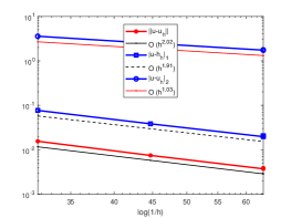
Fig. 17: Convergence rates of the plate bending problem for the $C^{1}$-continuous virtual elements

6.2 $C^{0}$-continuous VEMs

The Ref. [55] gives the $C^{0}$-continuous nonconforming virtual element method for the plate bending problem, with the local virtual element space defined as

$$V_{k}^{2,0}(K)=\{v\in H^{2}(K):\Delta^{2}v\in\mathbb{P}_{k-4}(K),~{}~{}v|_{\partial K}\in\mathbb{B}_{k}(\partial K)\},$$

where $K$ is a convex polygon and

$$\mathbb{B}_{k}(\partial K)=\{v\in C^{0}(\partial K):v|_{e}\in\mathbb{P}_{k}(e),~{}~{}\Delta v|_{e}\in\mathbb{P}_{k-2}(e),~{}~{}e\subset\partial K\}.$$

A function in $V_{k}^{2,0}(K)$ is uniquely identified by the following degrees of freedom:

• The values at the vertices of $K$,

  $$\chi_{i}(v)=v(z_{i}),\quad z_{i}~{}\mbox{is a vertex of $K$}.$$

• The moments of $v$ on edges up to degree $k-2$,

  $$\chi_{e}(v)=|e|^{-1}(m_{e},v)_{e},\quad v\in\mathbb{M}_{k-2}(e).$$

• The moments of $\partial_{\boldsymbol{n}}v$ on edges up to degree $k-2$,

  $$\chi_{n_{e}}(v)=(m_{e},\partial_{\boldsymbol{n}}v)_{e},\quad m\in\mathbb{M}_{k-2}(e).$$

• The moments of $v$ on $K$ up to degree $k-4$,

  $$\chi_{K}(v)=|K|^{-1}(m_{K},v)_{K},\quad v\in\mathbb{M}_{k-4}(K).$$

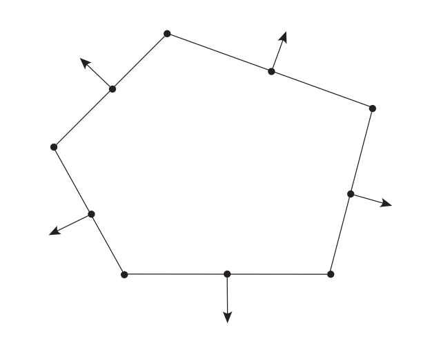
Fig. 18: Local degrees of freedom for the $C^{0}$-continuous virtual elements ($k=2$)

We only consider the lowest order case $k=2$. The d.o.f.s contain the values at the vertices and the following moments

$$\chi_{e}(v)=\frac{1}{|e|}\int_{e}v\mathrm{d}s,\quad\chi_{n_{e}}(v)=\int_{e}\partial_{\boldsymbol{n}}v\mathrm{d}s,$$

as shown in Fig. 18. Note that the first-type moments can also be replaced by the midpoint values on edges and the second-type moment has different signs when restricted to the left and right elements of an interior edge. Let $N_{v}$ be the number of vertices. Then there are $N_{k}=3N_{v}$ d.o.f.s on each element, arranged as

• The values at the vertices of $K$,

  $$\chi_{i}(v)=v(z_{i}),\quad i=1,\cdots,N_{v}.$$

• The mid-point values on each edge of $K$,

  $$\chi_{i+N_{v}}(v)=v(m_{i}),\quad i=1,\cdots,N_{v}.$$

• The moments

  $$\chi_{2N_{v}+i}(v)=\int_{e_{i}}\partial_{\boldsymbol{n}}v\mathrm{d}s,\quad i=1,\cdots,N_{v}.$$

Since

$$\int_{e}\partial_{\boldsymbol{n}}\phi^{T}\mathrm{d}s=[\boldsymbol{0},\boldsymbol{0},\boldsymbol{e}_{j}],\quad\phi^{T}(z_{i})=[\boldsymbol{e}_{i},\boldsymbol{0},\boldsymbol{0}],$$

the matrix $B$ for the elliptic projection can be realized as

⬇

1B = zeros(Nm,Ndof);

2p1 = [Nv,1:Nv-1]; p2 = 1:Nv;

3for j = 1:Nv % loop of edges

4 % nphi on ej

5 nphi = zeros(1,Ndof); nphi(2*Nv+j) = 1;

6 % Jump at zj

7 Jump = Mtn(:,p2(j))-Mtn(:,p1(j));

8 % phi at zj

9 phi = zeros(1,Ndof); phi(j) = 1;

10 % B1

11 B = B - Mnn(:,j)*nphi + Jump*phi;

12end

Noting that

$$\int_{\partial K}\nabla\phi_{j}\mathrm{d}s=\boldsymbol{t}_{e_{j-1}}-\boldsymbol{t}_{e_{j}},\quad\int_{\partial K}\nabla\phi_{N_{v}+j}\mathrm{d}s=\boldsymbol{0},\quad\int_{\partial K}\nabla\phi_{2N_{v}+j}\mathrm{d}s=\boldsymbol{n}_{e_{j}},$$

we can compute the constraints as follows.

⬇

1Bs = B;

2% first constraint

3Bs(1,1:Nv) = 1/Nv;

4% second constraint

5Bs(2:3,1:Nv) = te([Nv,1:Nv-1],:)' - te';

6Bs(2:3,2*Nv+1:end) = ne';

We repeat the test in Example 6.1 and display the result in Fig. 19. In this case, we still observe the optimal convergence rates. The test script is main_PlateBending_C0VEM.m.

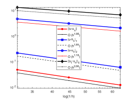
Fig. 19: Convergence rates of the plate bending problem for the $C^{0}$-continuous virtual elements

6.3 Morley-type VEMs

The fully $H^{2}$-nonconforming virtual element method was proposed in [3] for biharmonic problem. The local virtual element space is defined by

$$V_{k}^{2}(K) =\{v\in H^{2}(K):\Delta^{2}v\in\mathbb{P}_{k-4}(K),$$

$$\hskip 85.35826ptM_{\boldsymbol{nn}}(v)|_{e}\in\mathbb{P}_{k-2}(e),~{}~{}Q_{\boldsymbol{n}}(v)|_{e}\in\mathbb{P}_{k-3}(e),~{}~{}e\subset\partial K\}.$$

The corresponding degrees of freedom can be chosen as:

• The values at the vertices of $K$.

• The moments of $v$ on edges up to degree $k-3$,

  $$\chi_{e}(v)=|e|^{-1}(m_{e},v)_{e},\quad m_{e}\in\mathbb{M}_{k-3}(e).$$

• The moments of $\partial_{\boldsymbol{n}}v$ on edges up to degree $k-2$,

  $$\chi_{n_{e}}(v)=(m_{e},\partial_{\boldsymbol{n}}v)_{e},\quad m_{e}\in\mathbb{M}_{k-2}(e).$$

• The moments on element $K$ up to degree $k-4$,

  $$\chi_{K}(v)=|K|^{-1}(m_{K},v)_{K},\quad{m_{K}}\in\mathbb{M}_{k-4}(K).$$

If $k=2$ and $K$ is a triangle, one can prove that $V_{k}^{2}(K)$ becomes the well-known Morley element. We remark that the above Morley-type virtual element is also proposed in [56] with the same d.o.f.s but different local space, where the enhancement technique in [2] is utilized to modify the $C^{0}$-continuous spaces.

The test script is main_PlateBending_MorleyVEM.m. We repeat the test in Example 6.1 and display the result in Fig. 20, from which we again observe the optimal rate of convergence in all the discrete norms.

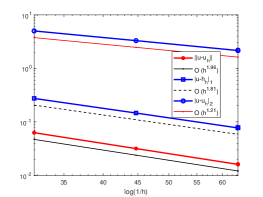
Fig. 20: Convergence rates of the plate bending problem for the fully nonconforming virtual elements

7 Stokes problem

The Stokes problem with homogeneous Dirichlet boundary conditions is to find $(\boldsymbol{u},p)$ such that

$$\begin{cases}-\nu\Delta\boldsymbol{u}-\nabla p=\boldsymbol{f}\quad&\mbox{in}~{}~{}\Omega,\\ {\rm div}\boldsymbol{u}=0\quad&\mbox{in}~{}~{}\Omega,\\ \boldsymbol{u}=\boldsymbol{0}\quad&\mbox{on}~{}~{}\partial\Omega.\end{cases}$$

Define

$$\boldsymbol{V}=\boldsymbol{H}_{0}^{1}(\Omega),\quad Q=L_{0}^{2}(\Omega).$$

The mixed variational problem is: Find $(\boldsymbol{u},p)\in\boldsymbol{V}\times Q$ such that

$$\begin{cases}a(\boldsymbol{u},\boldsymbol{v})+b(\boldsymbol{v},p)&=(\boldsymbol{f},\boldsymbol{v}),\quad\boldsymbol{v}\in\boldsymbol{V},\\ b(\boldsymbol{u},q)&=0,\quad q\in Q,\end{cases}$$

where

$$a(\boldsymbol{u},\boldsymbol{v})=(\nu\nabla\boldsymbol{u},\nabla\boldsymbol{v}),\qquad b(\boldsymbol{v},q)=({\rm div}\boldsymbol{v},q).$$

7.1 The mixed VEMs

In this subsection, we review the divergence-free virtual elements proposed in [17] for the Stokes problem.

7.1.1 Virtual element space and elliptic projection

The local virtual element space associated with $\boldsymbol{V}$ for $k\geq 2$ is

$$V_{k}(K) =\Big{\{}\boldsymbol{v}\in\boldsymbol{H}^{1}(K):\boldsymbol{v}|_{\partial K}\in[\mathbb{B}_{k}(\partial K)]^{2},$$

$$\hskip 85.35826pt\begin{cases}-\nu\Delta\boldsymbol{v}-\nabla s\in\mathcal{G}_{k-2}(K)^{\bot},\\ {\rm div}\boldsymbol{v}\in\mathbb{P}_{k-1}(K),\end{cases}\quad\mbox{for some $s\in L^{2}(K)$}\Big{\}},$$

where

$$\mathcal{G}_{k-2}(K)=\nabla(\mathbb{P}_{k-1}(K))\subset(\mathbb{P}_{k-2}(K))^{2}.$$

The finite dimensional space for $Q$ is taken as $Q_{k}(K)=\mathbb{P}_{k-1}(K)$.

The d.o.f.s for $V_{k}(K)$ and $Q_{k}(K)$ can be chosen as

• $\mathbb{D_{V}}1$: the values at the vertices of $K$.

• $\mathbb{D_{V}}2$: $k-1$ interior points on each edge $e$.

• $\mathbb{D_{V}}3$: the moments

  $$\int_{K}\boldsymbol{v}\cdot\boldsymbol{g}_{k-2}^{\bot}{\rm d}x,\quad\boldsymbol{g}_{k-2}^{\bot}\in\mathcal{G}_{k-2}(K)^{\bot}.$$

• $\mathbb{D_{V}}4$: the moments

  $$\int_{K}({\rm div}\boldsymbol{v})q_{k-1}{\rm d}x,\quad q_{k-1}\in\mathbb{P}_{k-1}(K)/\mathbb{R}.$$

• $\mathbb{D_{Q}}$: the moments

  $$\int_{K}qp_{k-1}{\rm d}x,\quad p_{k-1}\in\mathbb{P}_{k-1}(K).$$

As usual, we define the elliptic projection $\Pi^{K}:V_{k}(K)\to(\mathbb{P}_{k}(K))^{2}$, $\boldsymbol{v}\mapsto\Pi^{K}\boldsymbol{v}$ satisfying

$$\begin{cases}a^{K}(\Pi^{K}\boldsymbol{v},\boldsymbol{q})=a^{K}(\boldsymbol{v},\boldsymbol{q}),\quad\boldsymbol{q}\in(\mathbb{P}_{k}(K))^{2},\\ P_{0}^{K}(\Pi^{K}\boldsymbol{v})=P_{0}^{K}(\boldsymbol{v}),\end{cases}$$ (43)

where $P_{0}^{K}$ is the constant projector on $K$. One can check that the elliptic projection $\Pi^{K}\boldsymbol{v}$ is computable by using the given d.o.f.s. In fact, the integration by parts gives

$$a^{K}(\boldsymbol{v},\boldsymbol{q})=\int_{K}\nu\nabla\boldsymbol{q}\cdot\nabla\boldsymbol{v}{\rm d}x=-\int_{K}\nu\Delta\boldsymbol{q}\cdot\boldsymbol{v}{\rm d}x+\int_{\partial K}(\nu\nabla\boldsymbol{q}\boldsymbol{n})\cdot\boldsymbol{v}{\rm d}s,$$

where $\boldsymbol{n}=(n_{1},n_{2})^{T}$ and

$$\nabla\boldsymbol{q}=\begin{bmatrix}\nabla q_{1}\\ \nabla q_{2}\end{bmatrix}=\begin{bmatrix}q_{1,x}&q_{1,y}\\ q_{2,x}&q_{2,y}\end{bmatrix}.$$

Since $\nu\Delta\boldsymbol{q}\in(\mathbb{P}_{k-2}(K))^{2}$, there exists $q_{k-1}\in\mathbb{P}_{k-1}(K)/\mathbb{R}$ and $\boldsymbol{g}_{k-2}^{\bot}\in\mathcal{G}_{k-2}(K)^{\bot}$ such that

$$\nu\Delta\boldsymbol{q}=\nabla q_{k-1}+\boldsymbol{g}_{k-2}^{\bot}.$$

Then

$$a^{K}(\boldsymbol{v},\boldsymbol{q}) =-\int_{K}\nabla q_{k-1}\cdot\boldsymbol{v}{\rm d}x-\int_{K}\boldsymbol{g}_{k-2}^{\bot}\cdot\boldsymbol{v}{\rm d}x+\int_{\partial K}(\nu\nabla\boldsymbol{q}\boldsymbol{n})\cdot\boldsymbol{v}{\rm d}s$$

$$=\int_{K}q_{k-1}{\rm div}\boldsymbol{v}{\rm d}x-\int_{K}\boldsymbol{g}_{k-2}^{\bot}\cdot\boldsymbol{v}{\rm d}x+\int_{\partial K}(\nu\nabla\boldsymbol{q}\boldsymbol{n}-q_{k-1}\boldsymbol{n})\cdot\boldsymbol{v}{\rm d}s.$$ (44)

Obviously, the first term and the second term are determined by $\mathbb{D_{V}}4$ and $\mathbb{D_{V}}3$, respectively, while the boundary term can be computed by $\mathbb{D_{V}}1$ and $\mathbb{D_{V}}2$. Note that $\boldsymbol{g}_{k-2}^{\bot}=\boldsymbol{0}$ in the lowest order case $k=2$.

7.1.2 The discrete problem

The bilinear form $a^{K}(\boldsymbol{u},\boldsymbol{v})$ is approximated by

$$a_{h}^{K}(\boldsymbol{u},\boldsymbol{v})=a^{K}({\Pi}^{K}\boldsymbol{u},{\Pi}^{K}\boldsymbol{v})+S^{K}(\boldsymbol{u}-{\Pi}^{K}\boldsymbol{u},\boldsymbol{v}-{\Pi}^{K}\boldsymbol{v}),$$

with the stabilization term $S^{K}$ given by the $l^{2}$-inner product of the d.o.f. vectors.

In what follows we use $V_{h}$ to denote the global virtual element space of $V_{k}(K)$. The discrete space $Q_{h}$ of $Q$ is

$$Q_{h}:=\{q\in Q:q|_{K}\in\mathbb{P}_{k-1}(K),~{}~{}K\in\mathcal{T}_{h}.\}$$

The discrete mixed problem is: Find $(\boldsymbol{u}_{h},p_{h})\in V_{h}^{g}\times Q_{h}$ such that

$$\begin{cases}a_{h}(\boldsymbol{u}_{h},\boldsymbol{v}_{h})+b(\boldsymbol{v}_{h},p_{h})&=(\boldsymbol{f}_{h},\boldsymbol{v}_{h}),\quad\boldsymbol{v}_{h}\in V_{h},\\ b(\boldsymbol{u}_{h},q_{h})&=0,\quad q_{h}\in Q_{h}.\end{cases}$$ (45)

The constraint $\int_{\Omega}p_{h}{\rm d}x$ is not naturally imposed in the above system. To this end, we introduce a Lagrange multiplier and consider the augmented variational formulation: Find $((\boldsymbol{u}_{h},p_{h}),\lambda)\in V_{h}^{g}\times Q_{h}\times\mathbb{R}$ such that

$$\begin{cases}a_{h}(\boldsymbol{u}_{h},\boldsymbol{v}_{h})+b(\boldsymbol{v}_{h},p_{h})&=(\boldsymbol{f}_{h},\boldsymbol{v}_{h}),\quad\boldsymbol{v}_{h}\in V_{h},\\ \displaystyle b(\boldsymbol{u}_{h},q_{h})+\lambda\int_{\Omega}q_{h}{\rm d}x&=0,\quad q_{h}\in Q_{h},\\ \displaystyle\mu\int_{\Omega}p_{h}{\rm d}x&=0,\quad\mu\in\mathbb{R}.\end{cases}$$ (46)

Let $\boldsymbol{\phi}_{i}$, $i=1,\cdots,N$ be the basis functions of $V_{h}$. Then

$$\boldsymbol{u}=\sum\limits_{i=1}^{N}\chi_{i}(\boldsymbol{u})\boldsymbol{\phi}_{i}=:\boldsymbol{\phi}^{T}\boldsymbol{\chi}(\boldsymbol{u}).$$

Similarly, the basis functions of $Q_{h}$ are denote by $\psi_{l}$, $l=1,\cdots,M$, with

$$p_{h}=\sum\limits_{l=1}^{M}p_{l}\psi_{l}.$$

Plugging these expansions in (13) and taking $\boldsymbol{v}_{h}=\boldsymbol{\phi}_{j}$ and $q_{h}=\psi_{l}$, we obtain

$$\begin{cases}\sum\limits_{i=1}^{N}a_{h}(\boldsymbol{\phi}_{i},\boldsymbol{\phi}_{j})\chi_{i}+\sum\limits_{l=1}^{M}b(\boldsymbol{\phi}_{j},\psi_{l})p_{l}&=(\boldsymbol{f}_{h},\boldsymbol{\phi}_{j}),\quad j=1,\cdots,N,\\ \displaystyle\sum\limits_{i=1}^{N}b(\boldsymbol{\phi}_{i},\psi_{l})\chi_{i}+\lambda\int_{\Omega}\psi_{l}{\rm d}x&=0,\quad l=1,\cdots,M,\\ \displaystyle\sum\limits_{l=1}^{M}\int_{\Omega}\psi_{l}{\rm d}xp_{l}&=0.\end{cases}$$

Let

$$d_{l}=\int_{\Omega}\psi_{l}{\rm d}x,\quad\boldsymbol{d}=[d_{1},\cdots,d_{M}]^{T}.$$

The linear system can be written in matrix form as

$$\begin{bmatrix}A&B&\boldsymbol{0}\\ B^{T}&O&\boldsymbol{d}\\ \boldsymbol{0}^{T}&\boldsymbol{d}^{T}&0\end{bmatrix}\begin{bmatrix}\boldsymbol{\chi}\\ \boldsymbol{p}\\ \lambda\end{bmatrix}=\begin{bmatrix}\boldsymbol{f}\\ \boldsymbol{0}\\ 0\end{bmatrix},$$ (47)

where

$$A=(a_{h}(\boldsymbol{\phi}_{j},\boldsymbol{\phi}_{i})),\quad B=(b(\boldsymbol{\phi}_{j},\psi_{l})),\quad\boldsymbol{f}=((\boldsymbol{f}_{h},\boldsymbol{\phi}_{j})).$$

We only consider the lowest order case $k=2$. In this case, the third-type d.o.f.s vanish and the boundary part corresponds to a tensor-product space. We arrange the d.o.f.s in the following order:

$$\chi_{i}(\boldsymbol{v})=\boldsymbol{v}_{1}(z_{i}),\quad i=1,\cdots,N_{v},$$

$$\chi_{N_{v}+i}(\boldsymbol{v})=\boldsymbol{v}_{1}(m_{i}),\quad i=1,\cdots,N_{v},$$

$$\chi_{2*N_{v}+i}(\boldsymbol{v})=\boldsymbol{v}_{2}(z_{i}),\quad i=1,\cdots,N_{v},$$

$$\chi_{3N_{v}+i}(\boldsymbol{v})=\boldsymbol{v}_{2}(m_{i}),\quad i=1,\cdots,N_{v},$$

$$\chi_{4N_{v}+1}(\boldsymbol{v})=\int_{K}{\rm div}\boldsymbol{v}m_{2}(x,y){\rm d}x,\quad m_{2}(x,y)=\frac{x-x_{K}}{h_{K}},$$

$$\chi_{4N_{v}+2}(\boldsymbol{v})=\int_{K}{\rm div}\boldsymbol{v}m_{3}(x,y){\rm d}x,\quad m_{3}(x,y)=\frac{y-y_{K}}{h_{K}}.$$

Denote the basis functions of $\mathbb{B}_{k}(\partial K)$ by $\phi_{1},\cdots,\phi_{N_{v}};\phi_{N_{v}+1},\cdots,\phi_{2N_{v}}$. Then the tensor-product space $(\mathbb{B}_{k}(\partial K))^{2}$ has the basis functions:

$$\overline{\phi}_{1},\cdots,\overline{\phi}_{2N_{v}},\underline{\phi}_{1},\cdots,\underline{\phi}_{2N_{v}},$$

which correspond to the first $4N_{v}$ d.o.f.s. For convenience, we denote these functions by $\boldsymbol{\phi}_{1},\boldsymbol{\phi}_{2},\cdots,\boldsymbol{\phi}_{4N_{v}}$. The basis functions associated with the last two d.o.f.s are then denoted by $\boldsymbol{\varphi}_{1}=\boldsymbol{\phi}_{4N_{v}+1},\boldsymbol{\varphi}_{2}=\boldsymbol{\phi}_{4N_{v}+2}$.

In the following, we only provide the details of computing the elliptic projection.

7.2 Computation of the elliptic projection

7.2.1 Transition matrix

We rewrite the basis of $V_{k}(K)$ in a compact form as

$$\boldsymbol{\phi}^{T}=(\boldsymbol{\phi}_{1},\boldsymbol{\phi}_{2},\cdots,\boldsymbol{\phi}_{N_{k}}),$$

where $N_{k}=4N_{v}+2$ is the number of the d.o.f.s. The basis of $(\mathbb{P}_{k}(K))^{2}$ can be denote by

$$\boldsymbol{m}^{T}=(\boldsymbol{m}_{1},\boldsymbol{m}_{2},\cdots,\boldsymbol{m}_{N_{p}})=(\overline{m}_{1},\cdots,\overline{m}_{6},\underline{m}_{1},\cdots,\underline{m}_{6}).$$

Since $(\mathbb{P}_{k}(K))^{2}\subset V_{k}(K)$, one has $\boldsymbol{m}^{T}=\boldsymbol{\phi}^{T}\boldsymbol{D}$, where $\boldsymbol{D}$ is referred to as the transition matrix from $(\mathbb{P}_{k}(K))^{2}$ to $V_{k}(K)$. Let

$$\boldsymbol{m}^{T}=[{\overline{m}_{1}},{\overline{m}_{2}},{\overline{m}_{3}},{\underline{m}_{1}},{\underline{m}_{2}},{\underline{m}_{3}}]=:[\overline{m}^{T},\underline{m}^{T}],$$

$${\boldsymbol{\phi}^{T}}=[{\overline{\phi}_{1}},\cdots,{\overline{\phi}_{{N}}},{\underline{\phi}_{1}},\cdots,{\underline{\phi}_{{N}}},\boldsymbol{\varphi}_{1},\boldsymbol{\varphi}_{2}]=:[\overline{\phi}^{T},\underline{\phi}^{T},\boldsymbol{\varphi}_{1},\boldsymbol{\varphi}_{2}].$$

Blocking the matrix $\boldsymbol{D}$ as $\boldsymbol{D}=\begin{bmatrix}\boldsymbol{D}_{1}\\ \boldsymbol{D}_{2}\end{bmatrix}$, one has

$$\boldsymbol{m}=[\overline{m}^{T},\underline{m}^{T}] =[\overline{\phi}^{T},\underline{\phi}^{T},0,0]\boldsymbol{D}+[\boldsymbol{0}^{T},\boldsymbol{0}^{T},\boldsymbol{\varphi}_{1},\boldsymbol{\varphi}_{2}]\boldsymbol{D}$$

$$=[\overline{\phi}^{T},\underline{\phi}^{T},0,0]\begin{bmatrix}\boldsymbol{D}_{1}\\ \boldsymbol{O}\end{bmatrix}+[\boldsymbol{0}^{T},\boldsymbol{0}^{T},\boldsymbol{\varphi}_{1},\boldsymbol{\varphi}_{2}]\begin{bmatrix}\boldsymbol{O}\\ \boldsymbol{D}_{2}\end{bmatrix}.$$

Let $m^{T}=\phi^{T}D$. One easily finds that

$$\boldsymbol{D}_{1}=\begin{bmatrix}D&\\ &D\end{bmatrix},\qquad\boldsymbol{D}_{2}=\begin{bmatrix}\chi_{4N_{v}+1}(\overline{m}^{T})&\chi_{4N_{v}+1}(\underline{m}^{T})\\ \chi_{4N_{v}+2}(\overline{m}^{T})&\chi_{4N_{v}+2}(\underline{m}^{T})\end{bmatrix}$$

We first provide some necessary information.

⬇

1 % ------- element information ----------

2 index = elem{iel}; Nv = length(index);

3 xK = centroid(iel,1); yK = centroid(iel,2); hK = diameter(iel);

4 x = node(index,1); y = node(index,2);

5 v1 = 1:Nv; v2 = [2:Nv,1]; % loop index for vertices or edges

6 xe = (x(v1)+x(v2))/2; ye = (y(v1)+y(v2))/2; % mid-edge points

7 Ne = [y(v2)-y(v1), x(v1)-x(v2)]; % he*ne

8 nodeT = [node(index,:);centroid(iel,:)];

9 elemT = [(Nv+1)*ones(Nv,1),(1:Nv)',[2:Nv,1]'];

10

11 % --------------- scaled monomials -----------------

12 m1 = @(x,y) 1+0*x; gradm1 = @(x,y) [0+0*x, 0+0*x];

13 m2 = @(x,y) (x-xK)./hK; gradm2 = @(x,y) [1/hK+0*x, 0+0*x];

14 m3 = @(x,y) (y-yK)./hK; gradm3 = @(x,y) [0+0*x, 1/hK+0*x];

15 m4 = @(x,y) (x-xK).^2/hK^2; gradm4 = @(x,y) [2*(x-xK)./hK^2, 0+0*x];

16 m5 = @(x,y) (x-xK).*(y-yK)./hK^2; gradm5 = @(x,y) [(y-yK)./hK^2, (x-xK)./hK^2];

17 m6 = @(x,y) (y-yK).^2./hK^2; gradm6 = @(x,y) [0+0*x, 2*(y-yK)./hK^2];

18

19 m = @(x,y) [m1(x,y), m2(x,y), m3(x,y), m4(x,y), m5(x,y), m6(x,y)];

20 Gradm = {gradm1, gradm2, gradm3, gradm4, gradm5, gradm6};

21 divmm = @(x,y) [0+0*x, 1/hK+0*x, 0+0*x, 2*(x-xK)./hK^2, (y-yK)./hK^2, 0+0*x, ...

22 0+0*x, 0+0*x, 1/hK+0*x, 0+0*x, (x-xK)./hK^2, 2*(y-yK)./hK^2];

Then the transition matrix can be realized as

⬇

1 % -------- transition matrix ----------

2 NdofBd = 2*Nv; NdofA = 2*NdofBd+2;

3 divmm2 = @(x,y) divmm(x,y).*repmat(m2(x,y),1,Nmm);

4 divmm3 = @(x,y) divmm(x,y).*repmat(m3(x,y),1,Nmm);

5 D = zeros(NdofA, Nmm);

6 Dbd = [m(x,y); m(xe,ye)];

7 D(1:4*Nv, :) = blkdiag(Dbd, Dbd);

8 D(end-1,:) = integralTri(divmm2,4,nodeT,elemT);

9 D(end,:) = integralTri(divmm3,4,nodeT,elemT);

7.2.2 Elliptic projection matrices

The elliptic projection satisfies

$$\begin{cases}\boldsymbol{G}\boldsymbol{\Pi}_{*}^{K}=\boldsymbol{B},\\ P_{0}^{K}(\boldsymbol{m}^{T})\boldsymbol{\Pi}_{*}^{K}=P_{0}^{K}(\boldsymbol{\phi}^{T})\end{cases}\quad\mbox{or}\quad\tilde{\boldsymbol{G}}\boldsymbol{\Pi}_{*}^{K}=\tilde{\boldsymbol{B}},$$

where

$${\boldsymbol{G}}=a^{K}({\boldsymbol{m}},{\boldsymbol{m}}^{T}),\quad{\boldsymbol{B}}=a^{K}({\boldsymbol{m}},\boldsymbol{\phi}^{T}).$$

For $k=2$,

$${\boldsymbol{B}}_{\alpha i} =a^{K}({\boldsymbol{m}}_{\alpha},\boldsymbol{\phi}_{i})=\int_{K}q_{\alpha}{\rm div}\boldsymbol{\phi}_{i}{\rm d}x+\int_{\partial K}(\nu\nabla{\boldsymbol{m}}_{\alpha}\boldsymbol{n}-q_{\alpha}\boldsymbol{n})\cdot\boldsymbol{\phi}_{i}{\rm d}s$$

$$=:I_{1}(\alpha,i)+I_{2}(\alpha,i),$$

where

$$I_{1}(\alpha,i)=\int_{K}q_{\alpha}{\rm div}\boldsymbol{\phi}_{i}{\rm d}x,\quad I_{2}(\alpha,i)=\int_{\partial K}(\nu\nabla{\boldsymbol{m}}_{\alpha}\boldsymbol{n}-q_{\alpha}\boldsymbol{n})\cdot\boldsymbol{\phi}_{i}{\rm d}s,$$

and

$$\nu\Delta{\boldsymbol{m}}_{\alpha}=\nabla q_{\alpha}+0,\quad q_{\alpha}\in\mathbb{P}_{1}(K)/\mathbb{P}_{0}(K).$$

First consider $I_{1}$. By definition, let $q_{\alpha}=\nu h_{K}(c_{2,\alpha}m_{2}+c_{3,\alpha}m_{3})$. Then

$$\begin{bmatrix}c_{2,\alpha}\\ c_{3,\alpha}\end{bmatrix}\longleftarrow\begin{bmatrix}\Delta m^{T}&\boldsymbol{0}^{T}\\ \boldsymbol{0}^{T}&\Delta m^{T}\end{bmatrix}.$$

The Kronecher’s property gives

$$I_{1}(\alpha,i) =\nu h_{K}\Big{(}c_{2,\alpha}\int_{K}m_{2}{\rm div}\boldsymbol{\phi}_{i}{\rm d}x+c_{3,\alpha}\int_{K}m_{3}{\rm div}\boldsymbol{\phi}_{i}{\rm d}x\Big{)}$$

$$=\nu h_{K}\Big{(}c_{2,\alpha}\delta_{i,(4N_{v}+1)}+c_{3,\alpha}\delta_{i,(4N_{v}+2)}\Big{)}.$$

The computation of $I_{1}$ reads

⬇

1 % --- first term ---

2 Lapm = [0, 0, 0, 2/hK^2, 0, 2/hK^2];

3 B = zeros(Nmm, NdofA);

4 B(1:Nm, end-1) = pde.nu*hK*Lapm;

5 B(Nm+1:end, end) = pde.nu*hK*Lapm;

For the second term $I_{2}$, let $(g_{1}^{\alpha},g_{2}^{\alpha})^{T}=\nu\nabla{\boldsymbol{m}}_{\alpha}\boldsymbol{n}-q_{\alpha}\boldsymbol{n}$, Then

$$I_{2}(\alpha,i)=\int_{\partial K}g_{1}^{\alpha}\boldsymbol{\phi}_{1,i}{\rm d}s+\int_{\partial K}g_{2}^{\alpha}\boldsymbol{\phi}_{2,i}{\rm d}s=:J_{1}(\alpha,i)+J_{2}(\alpha,i).$$

Let $\phi$ be the basis of $\mathbb{B}_{k}(\partial K)$. One has

$$J_{1}(\alpha,:)^{T}=\begin{bmatrix}(g_{1}^{\alpha},\phi)_{\partial K}\\ (g_{1}^{\alpha},\boldsymbol{0})_{\partial K}\\ (g_{1}^{\alpha},\boldsymbol{\varphi}_{1,1})_{\partial K}\\ (g_{1}^{\alpha},\boldsymbol{\varphi}_{2,1})_{\partial K}\end{bmatrix}=\begin{bmatrix}(g_{1}^{\alpha},\phi)_{\partial K}\\ \boldsymbol{0}\\ 0\\ 0\end{bmatrix},$$

$$J_{2}(\alpha,:)^{T}=\begin{bmatrix}(g_{2}^{\alpha},\boldsymbol{0})_{\partial K}\\ (g_{2}^{\alpha},\phi)_{\partial K}\\ (g_{2}^{\alpha},\boldsymbol{\varphi}_{1,2})_{\partial K}\\ (g_{2}^{\alpha},\boldsymbol{\varphi}_{2,2})_{\partial K}\end{bmatrix}=\begin{bmatrix}\boldsymbol{0}\\ (g_{2}^{\alpha},\phi)_{\partial K}\\ 0\\ 0\end{bmatrix},$$

where $(g_{1}^{\alpha},\phi)_{\partial K}$ and $(g_{2}^{\alpha},\phi)_{\partial K}$ can be computed using the assembling technique for FEMs. For example, for $(g_{1}^{\alpha},\phi)_{\partial K}$ there exist three integrals on $e$:

$$F_{i}=\int_{e}g_{1}^{\alpha}\phi_{i}{\rm d}s,\quad i=1,2,3,$$

where $e=[a_{e},m_{e},b_{e}]$ is an edge with $a_{e}$ and $b_{e}$ being the endpoints and $m_{e}$ the midpoint. By the Simpson’s formula,

$$F=\begin{bmatrix}F_{1}\\ F_{2}\\ F_{3}\end{bmatrix}=\frac{h_{e}}{6}\begin{bmatrix}g_{1}^{\alpha}(a_{e})\\ g_{1}^{\alpha}(b_{e})\\ 4g_{1}^{\alpha}(m_{e})\end{bmatrix}.$$

The above discussion can be realized as follows.

⬇

1 % --- second term ---

2 elem1 = [v1(:), v2(:), v1(:)+Nv]; % elem2dof for [ae, be, me]

3 Gradmm = cell(2,Nmm);

4 Gradmm(1,1:Nm) = Gradm;

5 Gradmm(2,Nm+1:end) = Gradm;

6 for im = 1:Nm

7 Gradmm{1,im+Nm} = @(x,y) [0+0*x, 0+0*x];

8 Gradmm{2,im} = @(x,y) [0+0*x, 0+0*x];

9 end

10 qmm = cell(1,Nmm); % q = nu*hK(c2*m2 + c3*m3)

11 c2 = [Lapm, zeros(1,Nm)];

12 c3 = [zeros(1,Nm), Lapm];

13 for im = 1:Nmm

14 qmm{im} = @(x,y) pde.nu*hK*(c2(im)*m2(x,y) + c3(im)*m3(x,y));

15 end

16 for s = 1:2

17 id = (1:NdofBd) + (s-1)*NdofBd;

18 for im = 1:Nmm

19 pm = @(x,y) pde.nu*Gradmm{s,im}(x,y);

20 qa = @(x,y) qmm{im}(x,y);

21 F1 = 1/6*(sum(pm(x(v1),y(v1)).*Ne, 2) - qa(x(v1),y(v1)).*Ne(:,s));

22 F2 = 1/6*(sum(pm(x(v2),y(v2)).*Ne, 2) - qa(x(v2),y(v2)).*Ne(:,s));

23 F3 = 4/6*(sum(pm(xe,ye).*Ne, 2) - qa(xe,ye).*Ne(:,s));

24 B(im, id) = accumarray(elem1(:), [F1; F2; F3], [NdofBd, 1]);

25 end

26 end

We finally consider the implementation of the constraint. At first glance the $L^{2}$ projection is not computable since there is no zero-order moment on $K$. In fact, the computability can be obtained using the decomposition of polynomial spaces. Let $\boldsymbol{\phi}_{i}=[\boldsymbol{\phi}_{1,i},\boldsymbol{\phi}_{1,i}]^{T}$. Then

$$\boldsymbol{\phi}_{1,i}=\boldsymbol{\phi}_{i}\cdot\begin{bmatrix}1\\ 0\end{bmatrix},\quad\boldsymbol{\phi}_{2,i}=\boldsymbol{\phi}_{i}\cdot\begin{bmatrix}0\\ 1\end{bmatrix}.$$

It is easy to get

$$\begin{bmatrix}1\\ 0\end{bmatrix}=\nabla p_{k-1}+\boldsymbol{g}_{k-2}^{\bot},\quad p_{k-1}=h_{K}m_{2},\quad\boldsymbol{g}_{k-2}^{\bot}=\boldsymbol{0},$$

$$\begin{bmatrix}0\\ 1\end{bmatrix}=\nabla q_{k-1}+\boldsymbol{g}_{k-2}^{\bot},\quad q_{k-1}=h_{K}m_{3},\quad\boldsymbol{g}_{k-2}^{\bot}=\boldsymbol{0},$$

which yield

$$P_{0}^{K}(\boldsymbol{\phi}_{1,i})=|K|^{-1}\int_{K}\boldsymbol{\phi}_{i}\cdot\nabla p_{k-1}{\rm d}x=|K|^{-1}h_{K}\Big{(}-\int_{K}{\rm div}\boldsymbol{\phi}_{i}m_{2}{\rm d}x+\int_{\partial K}m_{2}\boldsymbol{\phi}_{i}\cdot\boldsymbol{n}{\rm d}s\Big{)},$$

$$P_{0}^{K}(\boldsymbol{\phi}_{2,i})=|K|^{-1}\int_{K}\boldsymbol{\phi}_{i}\cdot\nabla q_{k-1}{\rm d}x=|K|^{-1}h_{K}\Big{(}-\int_{K}{\rm div}\boldsymbol{\phi}_{i}m_{3}{\rm d}x+\int_{\partial K}m_{3}\boldsymbol{\phi}_{i}\cdot\boldsymbol{n}{\rm d}s\Big{)}.$$ (48)

As you can see, their computation is similar to the previous one for $B_{\alpha,i}$ with $\alpha$ fixed. The resulting two row vectors will replace the first and seventh rows of $B$.

⬇

1 % constraint

2 P0K = zeros(2,NdofA);

3 P0K(1, end-1) = -1; P0K(2, end) = -1;

4 m23 = {m2, m3};

5 for s = 1:2

6 mc = m23{s};

7 F1 = 1/6*(mc(x(v1),y(v1)).*Ne); % [n1, n2]

8 F2 = 1/6*(mc(x(v2),y(v2)).*Ne);

9 F3 = 4/6*(mc(xe,ye).*Ne);

10 F = [F1; F2; F3];

11 P0K(s, 1:NdofBd) = accumarray(elem1(:), F(:,1), [NdofBd 1]);

12 P0K(s, NdofBd+1:2*NdofBd) = accumarray(elem1(:), F(:,2), [NdofBd 1]);

13 end

14 P0K = 1/area(iel)*hK*P0K;

15 % Bs, G, Gs

16 Bs = B; Bs([1,7], :) = P0K;

Example 7.1.

Let $\Omega=(0,1)^{2}$. We choose the load term $\boldsymbol{f}$ in such a way that the analytical solution is

$$\boldsymbol{u}(x,y)=\begin{bmatrix}-\frac{1}{2}\cos(x)^{2}\cos(y)\sin(y)\\ \frac{1}{2}\cos(y)^{2}\cos(x)\sin(x)\end{bmatrix},\quad p(x,y)=\sin(x)-\sin(y).$$

The results are displayed in Fig. 21 and Tab. 3, from which we observe the optimal rates of convergence both for $u$ and $p$.

Fig. 21: Convergence rates of the divergence free VEM for the Stokes problem

Tab. 3: The discrete errors for the Stokes problem

$\sharp$Dof	$h$	$\|u-u_{h}\|$	$|u-u_{h}|_{1}$	$\|p-p_{h}\|$
390	1.768e-01	1.07945e-04	3.25802e-03	5.66765e-03
774	1.250e-01	5.16780e-05	1.55844e-03	2.84772e-03
1534	8.839e-02	2.13132e-05	7.72427e-04	1.45175e-03
3042	6.250e-02	1.00841e-05	3.84674e-04	7.33126e-04
6090	4.419e-02	5.69480e-06	1.93534e-04	3.68775e-04

8 Adaptive virtual element methods

Due to the large flexibility of the meshes, researchers have focused on the a posterior error analysis of the VEMs and made some progress in recent years [18, 24, 20, 29, 19, 37].

We consider the adaptive VEMs for the Poisson equation. The computable error estimator is taken from [20, 37], given as

$$\eta(u_{h})=\Big{(}\sum\limits_{K\in\mathcal{T}_{h}}\eta_{K}^{2}(u_{h})\Big{)}^{1/2},$$

where

$$\eta_{K}^{2}(u_{h})=\sum\limits_{i=1}^{4}\eta_{i,K}^{2}(u_{h}),$$

with

$$\eta_{1,K}^{2}=h_{K}^{2}\|f-\Pi_{0}^{K}f\|_{0,K}^{2},\quad\eta_{2,K}^{2}=h_{K}^{2}\|\Pi_{0}^{K}f\|_{0,K}^{2},\quad\eta_{3,K}^{2}=\|\boldsymbol{\chi}(u_{h}-\Pi_{1}^{\nabla}u_{h})\|_{l^{2}}^{2},$$

and

$$\eta_{4,K}^{2}=\frac{1}{2}\sum\limits_{e\subset\partial K}h_{e}\|[\partial_{\boldsymbol{n}}\Pi_{1}^{\nabla}u_{h}]\|_{0,e}^{2}.$$

Standard adaptive algorithms based on the local mesh refinement can be written as loops of the form

$${\bf SOLVE}\to{\bf ESTIMATE}\to{\bf MARK}\to{\bf REFINE}.$$

Given an initial polygonal subdivision $\mathcal{T}_{0}$, to get $\mathcal{T}_{k+1}$ from $\mathcal{T}_{k}$ we first solve the VEM problem under consideration to get the numerical solution $u_{k}$ on $\mathcal{T}_{k}$. The error is then estimated by using $u_{k}$, $\mathcal{T}_{k}$ and the a posteriori error bound. The local error bound is used to mark a subset of elements in $\mathcal{T}_{k}$ for refinement. The marked polygons and possible more neighboring elements are refined in such a way that the subdivision meets certain conditions, for example, the resulting polygonal mesh is still shape regular. In the implementation, it is usually time-consuming to write a mesh refinement function since we need to carefully design the rule for dividing the marked elements to get a refined mesh of high quality. We have present such an implementation of the mesh refinement for polygonal meshes in [52].

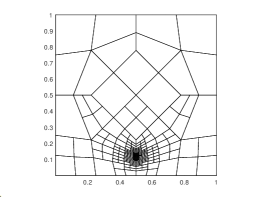
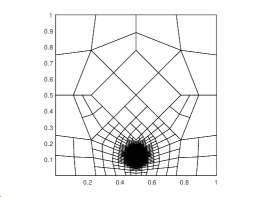
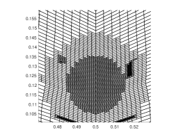
Fig. 22: The initial and the final adapted meshes. (a) The initial mesh; (b) After 20 refinement steps; (c) After 30 refinement steps; (d) The zoomed mesh in (c)

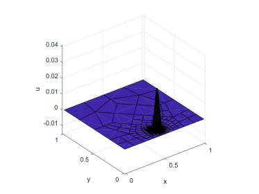
(a) Exact

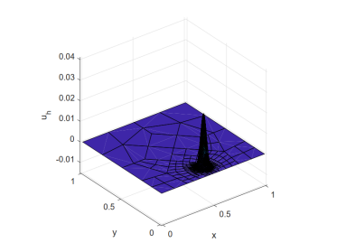
(b) Numerical

Fig. 23: The exact and numerical solutions

Consider the Poisson equation with Dirichlet boundary condition on the unit square. The exact solution is given by

$$u(x,y)=xy(1-x)(1-y){\text{exp}}\left(-1000((x-0.5)^{2}+(y-0.117)^{2})\right).$$

We employ the VEM in the lowest order case and use the Dörfler marking strategy with parameter $\theta=0.4$ to select the subset of elements for refinement. The initial mesh and the final adapted meshes after 20 and 30 refinement steps are presented in Fig. 22 (a-c), respectively. The detail of the last mesh is shown in Fig. 22 (d). Clearly, no small edges are observed. We also plot the adaptive approximation in Fig. 23, which almost coincides with the exact solution. The full code is available from mVEM package. The subroutine PoissonVEM_indicator.m is used to compute the local indicator and the test script is main_Poisson_avem.m. As shown in Fig. 24, we see the adaptive strategy correctly refines the mesh in a neighborhood of the singular point and there is a good level of agreement between the $H^{1}$ error and error estimator.

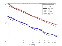
Fig. 24: Convergence rates of the error $|u-\Pi_{1}^{\nabla}u_{h}|_{1}$ and the error estimator $\eta(u_{h})$

9 Variational inequalities

We now focus on the the virtual element method to solve a simplified friction problem, which is a typical elliptic variational inequality of the second kind.

9.1 The simplified friction problem

Let $\Omega\subset\mathbb{R}^{2}$ be a bounded domain with a Lipschitz boundary $\Gamma=\partial\Omega$ that is divided into two parts $\Gamma_{C}$ and $\Gamma_{D}$. The problem is

$$\begin{cases}-\Delta u+\alpha u=f\quad&\mbox{in}~{}~{}\Omega,\\ \partial_{\boldsymbol{n}}u\leq g,\quad u\partial_{\boldsymbol{n}}u+g|u|=0,\quad&\mbox{on}~{}~{}\Gamma_{C},\\ u=0\quad\mbox{on}~{}~{}&\Gamma_{D},\end{cases}$$ (49)

where $\alpha>0$ is a constant, $f\in L^{2}(\Omega)$, $g\in L^{2}(\Gamma_{C})$, $\Gamma_{C}$ is the frictional boundary part and $\Gamma_{D}$ is the Dirichlet boundary part.

Define

$$V=\{v\in H^{1}(\Omega):v|_{\Gamma_{D}}=0\}.$$

The variational inequality is [48]: Find $u\in V$ such that

$$a(u,v-u)+j(v)-j(u)\geq\ell(v-u),\quad v\in V,$$ (50)

where

$$a(u,v)=\int_{\Omega}(\nabla u\cdot\nabla v+\alpha uv){\rm d}x,\quad\ell(v)=\int_{\Omega}fv{\rm d}x,\quad j(v)=\int_{\Gamma_{C}}g|v|{\rm d}s.$$

9.2 The VEM discretization

We consider the lowest-order virtual element space. The local space is taken as the enhanced virtual element space $W_{1}(K)$ defined in (23). Let $V_{h}$ be the global space. The virtual element method for solving the simplified friction problem is: Find $u_{h}\in V_{h}$ such that

$$a_{h}(u_{h},v_{h}-u_{h})+j(v_{h})-j(u_{h})\geq\ell_{h}(v_{h}-u_{h}),\quad v_{h}\in V_{h},$$ (51)

where

$$a_{h}^{K}(v,w)=(\nabla\Pi_{1}^{\nabla}v,\nabla\Pi_{1}^{\nabla}w)_{K}+\alpha(\Pi_{1}^{0}v,\Pi_{1}^{0}w)_{K}+S^{K}(v-\Pi_{1}^{\nabla}v,w-\Pi_{1}^{\nabla}w),$$

$$S^{K}(v,w):=(1+\alpha h_{K}^{2})\boldsymbol{\chi}(v)\cdot\boldsymbol{\chi}(w),\quad\ell_{h}(v_{h})=\sum\limits_{K\in\mathcal{T}_{h}}(f,\Pi_{0}^{0}v_{h})_{K}.$$

By introducing a Lagrangian multiplier

$$\lambda\in\Lambda=\{\lambda\in L^{\infty}(\Gamma_{C}):|\lambda|\leq 1\quad\mbox{a.e.~{}~{}on}~{}~{}\Gamma_{C}\},$$

the inequality problem (50) can be rewritten as

$$\begin{cases}a(u,v)+\displaystyle\int_{\Gamma_{C}}g\lambda v{\rm d}s=\ell(v),\quad&v\in V,\\ \lambda u=|u|\quad\mbox{a.e.~{}~{}on}~{}~{}\Gamma_{C}.\end{cases}$$

For this reason, the discrete problem (51) can be recast as

$$\begin{cases}a_{h}(u_{h},v_{h})+\displaystyle\int_{\Gamma_{C}}g\lambda_{h}v_{h}{\rm d}s=\ell_{h}(v_{h}),\quad&v_{h}\in V_{h},\\ \lambda_{h}u_{h}=|u_{h}|\quad\mbox{a.e.~{}~{}on}~{}~{}\Gamma_{C},\end{cases}$$

where $\lambda_{h}\in L^{\infty}(\Gamma_{C})$ and $|\lambda_{h}|\leq 1$. Then the Uzawa algorithm for solving the above problem is [50, 51]: given any $\lambda_{h}^{(0)}\in\Lambda$, for $n\geq 1$, find $u_{h}^{(n)}$ and $\lambda_{h}^{(n)}$ by solving

$$a_{h}(u_{h}^{(n)},v_{h})=\ell_{h}(v_{h})-\int_{\Gamma_{C}}g\lambda_{h}^{(n-1)}v_{h}{\rm d}s$$ (52)

and

$$\lambda_{h}^{(n)}=P_{\Lambda}(\lambda_{h}^{(n-1)}+\rho gu_{h}^{(n)}),$$

where $P_{\Lambda}(\mu)=\sup\{-1,\inf\{1,\mu\}\}$ and $\rho$ is a constant parameter.

9.3 Numerical example

Let $\Omega=(0,1)^{2}$ and suppose that the frictional boundary condition is imposed on $y=0$. The function $g$ can be simply chosen as $\sup_{\Gamma_{C}}|\partial_{\boldsymbol{n}}u|$. The right-hand function $f$ is chosen such that the exact solution is $u=(\sin(x)-x\sin(1))\sin(2\pi y)$.

The Uzawa iteration stops when $\|\boldsymbol{\chi}(u_{h}^{n+1}-u_{h}^{n})\|_{l^{2}}\leq\mbox{tol}$ or $n\geq\mbox{maxIt}$. It is evident that the problem (52) is exactly the VEM discretization for the reaction-diffusion problems, with the Neumann boundary data replaced by $g\lambda_{h}^{(n-1)}$. In addition, we only need to assemble the integral on $\Gamma_{C}$ in each iteration. Because of this, we will not give the implementation details. We set $\mbox{tol}=10^{-8}$, $\mbox{maxIt}=500$ and $\rho=10$. The results are shown in Figs. 25 and 26, from which we see that the lowest-order VEM achieves the linear convergence order in the discrete $H^{1}$ norm, which is optimal according to the a priori error estimate in [48]. The test script is main_PoissonVEM_VI_Uzawa.m.

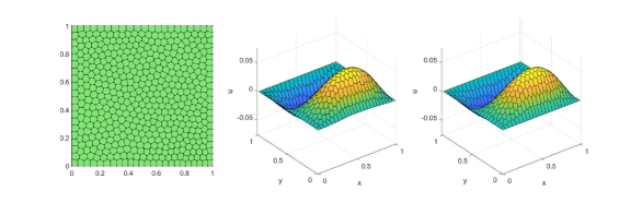
Fig. 25: Numerical and exact solutions for the simplified friction problem ($\alpha=10^{4}$)

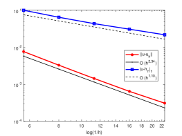
Fig. 26: Convergence rates of the VEM for the simplified friction problem ($\alpha=10^{4}$)

10 Three-dimensional problems

In this section we are concerned with the implementation of 3-D VEMs proposed in [15] for the Poisson equation in the lowest-order case. Considering the length of the article, we omit the details of the introduction to the function spaces.

10.1 Virtual element methods for the 3-D Poisson equation

Let $\Omega\subset\mathbb{R}^{3}$ be a polyhedral domain and let $\Gamma$ denote a subset of its boundary consisting of some faces. We consider the following model problem

$$\begin{cases}-\Delta u=r\quad&\mbox{in}~{}~{}\Omega,\\ u=g_{D}\quad&\mbox{on}~{}~{}\Gamma,\\ \partial_{n}u=g_{N}\quad&\mbox{on}~{}~{}\Gamma^{\prime}=\partial\Omega\backslash\Gamma,\end{cases}$$ (53)

where $r\in L^{2}(\Omega)$ and $g_{N}\in L^{2}(\Gamma^{\prime})$ are the applied load and Neumann boundary data, respectively, and $g_{D}\in H^{1/2}(\Gamma)$ is the Dirichlet boundary data function.

In what follows, we use $K$ to represent the generic polyhedral element with $f\subset\partial K$ being its generic face. The vertices of a face $f$ are in a counterclockwise order when viewed from the inside. The virtual element method proposed in [15] for (53) is to find $u_{h}\in V_{\Gamma}^{k}$ such that

$$a_{h}(u_{h},v_{h})=\ell_{h}(v_{h}),\quad v_{h}\in V_{0}^{k},$$

where

$$a_{h}(u_{h},v_{h})=\sum\limits_{K\in\mathcal{T}_{h}}a_{h}^{K}(u_{h},v_{h}),\quad\ell_{h}(v_{h})=\int_{\Omega}r_{h}v_{h}{\rm d}x+\int_{\Gamma^{\prime}}g_{h}v_{h}{\rm d}s.$$

The local bilinear form is split into two parts:

$$a_{h}^{K}(v,w)=(\nabla\Pi_{1}^{\nabla}v,\nabla\Pi_{1}^{\nabla}w)_{K}+h_{K}S^{K}(v-\Pi_{1}^{\nabla}v,w-\Pi_{1}^{\nabla}w),$$

where $\Pi_{1}^{\nabla}:V^{1}(K)\to\mathbb{P}_{1}(K)$ is the elliptic projector and $S^{K}$ is the stabilization term given as

$$S^{K}(v,w)=\sum\limits_{i=1}^{N^{K}}\chi_{i}(v)\chi_{i}(w),$$

where $\chi_{i}(v)=v(p_{i})$ and $p_{i}$ is the $i$-th vertex of $K$ for $i=1,2,\cdots,N_{K}$. The local linear form of the right-hand side will be approximated as

$$\ell_{h}^{K}(v_{h})=\int_{K}r\Pi_{1}^{\nabla}v_{h}{\rm d}x+\sum\limits_{f\subset\Gamma^{\prime}\cap\partial K}\int_{f}g_{N}\Pi_{1,f}^{\nabla}v_{h}{\rm d}s,$$

where $\Pi_{1,f}^{\nabla}:V^{1}(f)\to\mathbb{P}_{1}(f)$ is the elliptic projector defined on the face $f$.

For the detailed introduction of the virtual element spaces, please refer to Section 2 in [15]. In this paper, we only consider the lowest-order case, but note that the hidden ideas can be directly generalized to higher order cases.

10.2 Data structure and test script

We first discuss the data structure to represent polyhedral meshes. In the implementation, the mesh is represented by node3 and elem3. The ${\leavevmode\lstinline{{\lst@@@set@language\lst@@@set@numbers\lst@@@set@frame\lst@@@set@rulecolor\lst@@@set@language\lst@@@set@numbers\lst@@@set@frame\lst@@@set@rulecolor\lst@@@set@language\lst@@@set@numbers\lst@@@set@frame\footnotesize\small{\@listingGroup{ltx_lst_identifier}{N}}}}}\times 3$ matrix node3 stores the coordinates of all vertices in the mesh. elem3 is a cell array with each entry storing the face connectivity, for example, the first entry elemf = elem3{1} for the mesh given in Fig. 27(a) is shown in Fig. 27(b), which is still represented by a cell array since the faces may have different numbers of vertices.

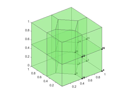
(a) Polyhedral mesh

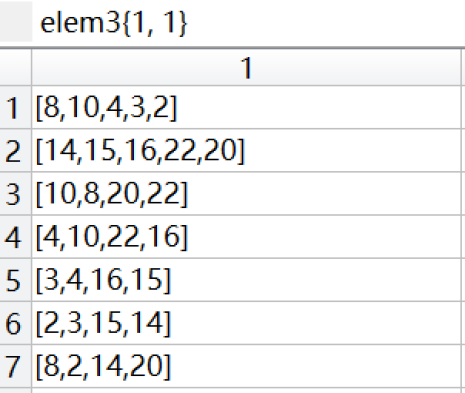
(b) Representation of the first element

Fig. 27: Polyhedral mesh of a cube

All faces including the repeated internal ones can be gathered in a cell array as

allFace = vertcat(elem3{:}); % cell

By padding the vacancies and using the sort and unique functions to rows, we obtain the face set face. The cell array elem2face then establishes the map of local index of faces in each polyhedron to its global index in face set face. The above structural information is summarized in the subroutine auxstructure3.m. The geometric quantities such as the diameter diameter3, the barycenter centroid3 and the volume volume are computed by auxgeometry3.m. We remark that these two subroutines may be needed to add more information when dealing with higher order VEMs.

The test script is main_PoissonVEM3.m listed as follows. In the for loop, we first load the pre-defined mesh data, which immediately returns the matrix node3 and the cell array elem3 to the MATLAB workspace. Then we set up the Neumann boundary conditions to get the structural information of the boundary faces. The subroutine PoissonVEM3.m is the function file containing all source code to implement the 3-D VEM. When obtaining the numerical solutions, we calculate the discrete $L^{2}$ errors and $H^{1}$ errors defined as

$$\mbox{ErrL2}=\sum\limits_{K\in\mathcal{T}_{h}}\|u-\Pi_{1}^{\nabla}u_{h}\|_{0,K},\quad\mbox{ErrH1}=\sum\limits_{K\in\mathcal{T}_{h}}|u-\Pi_{1}^{\nabla}u_{h}|_{1,K}$$

by using respectively the subroutine getError3.m. The procedure is completed by verifying the rate of convergence through showrateErr.m.

⬇

1%% Parameters

2maxIt = 5;

3h = zeros(maxIt,1); N = zeros(maxIt,1);

4ErrL2 = zeros(maxIt,1); ErrH1 = zeros(maxIt,1);

5

6%% PDE data

7pde = Poisson3data();

8bdNeumann = 'x==0'; % string for Neumann

9

10%% Virtual element method

11for k = 1:maxIt

12 % load mesh

13 fprintf('Mesh %d: \n', k);

14 load( ['SimpleMesh3data', num2str(k), '.mat'] ); % polyhedral mesh

15 %load( ['mesh3data', num2str(k), '.mat'] ); % polyhedral mesh

16 %[node3,$\neg$,elem3] = cubemesh([0 1 0 1 0 1], 1/(2*k)); % tetrahedral mesh

17 % get boundary information

18 bdStruct = setboundary3(node3,elem3,bdNeumann);

19 % solve

20 [uh,info] = PoissonVEM3(node3,elem3,pde,bdStruct);

21 % record

22 N(k) = length(uh); h(k) = (1/size(elem3,1))^(1/3);

23 % compute errors in discrete L2, H1 and energy norms

24 kOrder = 1;

25 [ErrH1(k),ErrL2(k)] = getError3(node3,elem3,uh,info,pde,kOrder);

26end

27

28%% Plot convergence rates and display error table

29figure, showrateErr(h,ErrL2,ErrH1);

30

31fprintf('\n');

32disp('Table: Error')

33colname = {'#Dof','h','||u-u_h||','|u-u_h|_1'};

34disptable(colname,N,[],h,'%0.3e',ErrL2,'%0.5e',ErrH1,'%0.5e');

In the following subsections, we shall go into the details of the implementation of the 3-D VEM in PoissonVEM3.m.

10.3 Elliptic projection on polygonal faces

Let $f$ be a face of $K$ or a polygon embedded in $\mathbb{R}^{3}$. In the VEM computing, we have to get all elliptic projections $\Pi_{1,f}^{\nabla}\phi_{f}^{T}$ ready in advance, where $\phi_{f}$ is the nodal basis of the enhanced virtual element space $V^{1}(f)$ (see Subsection 2.3 in [15]). To this end, it may be necessary to establish local coordinates $(s,t)$ on the face $f$.

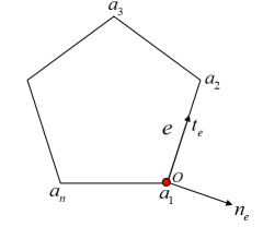
Fig. 28: Local coordinate system of a face or polygon embedded in $\mathbb{R}^{3}$

As shown in Fig. 28, the boundary of the polygon is oriented in a counterclockwise order as $a_{1},\cdots,a_{n}$. Let $e=a_{1}a_{2}$ be the first edge, and $n_{e}$ and $t_{e}$ be the normal vector and tangential vector, respectively. Then we can define a local coordinate system with $a_{1}$ being the original point by using these two vectors. Let $n_{e}=(n_{1},n_{2},n_{3})$ and $t_{e}=(t_{1},t_{2},t_{3})$. For any $a=(x,y,z)\in f$, its local coordinate $(s,t)$ is related by

$$\overrightarrow{Oa}=s\cdot n_{e}+t\cdot t_{e},\quad\mbox{or}\quad(x-x_{1},y-y_{1},z-z_{1})=s\cdot(n_{1},n_{2},n_{3})+t\cdot(t_{1},t_{2},t_{3}),$$

which gives

$$(s,t)=(x-x_{1},y-y_{1},z-z_{1})\begin{bmatrix}n_{1}&n_{2}&n_{3}\\ t_{1}&t_{2}&t_{2}\end{bmatrix}^{-1},$$

with the inverse understood in the least squares sense. When converting to the local coordinate system, we can compute all the matrices of elliptic projection in the same way for the Poisson equation in two-dimensional cases. For completeness, we briefly recall the implementation. In what follows, we use the subscript “$f$” to indicate the locally defined symbols.

Let $\phi_{f}^{T}=[\phi_{f,1},\cdots,\phi_{f,n}]$ be the basis functions of $V^{1}(f)$ and $m_{f}^{T}=[m_{f,1},m_{f,2},m_{f,3}]$ the scaled monomials on $f$ given as

$$m_{f,1}=1,\quad m_{f,2}=\frac{s-s_{f}}{h_{f}},\quad m_{f,3}=\frac{t-t_{f}}{h_{f}},$$

where $(s_{f},t_{f})$ and $h_{f}$ are the barycenter and the diameter of $f$, respectively. The vector form of the elliptic projector $\Pi_{1,f}^{\nabla}$ can be represented as

$$\begin{cases}(\nabla_{f}m_{f},\nabla_{f}\Pi_{1,f}^{\nabla}\phi_{f}^{T})_{f}=(\nabla_{f}m_{f},\nabla_{f}\phi_{f}^{T})_{f},\\ P_{0}(\Pi_{1,f}^{\nabla}\phi_{f}^{T})=P_{0}(\phi_{f}^{T}).\end{cases}$$ (54)

where

$$P_{0}(v)=\frac{1}{n}\sum\limits_{i=1}^{n}v(a_{i}).$$

Since $\mathbb{P}_{1}(f)\subset V^{1}(f)$, we can write

$$m_{f}^{T}=\phi_{f}^{T}\boldsymbol{D}_{f},\qquad\boldsymbol{D}_{f}=(D_{i\alpha}),\quad D_{i\alpha}=\chi_{f,i}(m_{f,\alpha}),$$

where $\chi_{f,i}$ is the $i$-th d.o.f associated with $a_{i}$, and $\boldsymbol{D}_{f}$ is referred to as the transition matrix. We further introduce the following expansions

$$\Pi_{1,f}^{\nabla}{\phi_{f}^{T}}=\phi_{f}^{T}\boldsymbol{\Pi}_{1,f}^{\nabla},\qquad\Pi_{1,f}^{\nabla}{\phi_{f}^{T}}=m_{f}^{T}\boldsymbol{\Pi}_{1*,f}^{\nabla}.$$

One easily finds that

$$\boldsymbol{\Pi}_{1,f}^{\nabla}=\boldsymbol{D}_{f}\boldsymbol{\Pi}_{1*,f}^{\nabla},$$

and (54) can be rewritten in matrix form as

$$\begin{cases}\boldsymbol{G}_{f}\boldsymbol{\Pi}_{1*,f}^{\nabla}=\boldsymbol{B}_{f},\\ P_{0}(m_{f}^{T})\boldsymbol{\Pi}_{1*,f}^{\nabla}=P_{0}(\phi_{f}^{T})\end{cases},\quad\mbox{or denoted by}\quad\tilde{\boldsymbol{G}}_{f}\boldsymbol{\Pi}_{1*,f}^{\nabla}=\tilde{\boldsymbol{B}}_{f},$$

where

$$\boldsymbol{G}_{f}=(\nabla_{f}m_{f},\nabla_{f}m_{f}^{T})_{f},\quad\boldsymbol{B}_{f}=(\nabla_{f}m_{f},\nabla_{f}\phi_{f}^{T})_{f}.$$

Note that the following consistency relation holds

$$\boldsymbol{G}_{f}=\boldsymbol{B}_{f}\boldsymbol{D}_{f},\quad\tilde{\boldsymbol{G}}_{f}=\tilde{\boldsymbol{B}}_{f}\boldsymbol{D}_{f}.$$

Let face be the face set with internal faces repeated once. Then using the local coordinates we are able to derive all elliptic projections $\Pi_{1,f}^{\nabla}\phi_{f}^{T}$ as in 2-D cases. It is not recommended to carry out the calculation element by element in view of the repeated cost for the internal faces.

The above discussion is summarized in a subroutine with input and output as

Pifs = faceEllipticProjection(P),

where P is the coordinates of the face $f$ and Pifs is the matrix representation $\boldsymbol{\Pi}_{1*,f}^{\nabla}$ of $\Pi_{1,f}^{\nabla}\phi_{f}^{T}$ in the basis $m_{f}^{T}$. One can derive all matrices by looping over the face set face:

⬇

1%% Derive elliptic projections of all faces

2faceProj = cell(NF,1);

3for s = 1:NF

4 % Pifs

5 faces = face{s}; P = node3(faces,:);

6 Pifs = faceEllipticProjection(P);

7 % sort the columns

8 [$\neg$,idx] = sort(faces);

9 faceProj{s} = Pifs(:,idx);

10end

Note that in the last step we sort the columns of $\boldsymbol{\Pi}_{1*,f}^{\nabla}$ in ascending order according to the numbers of the vertices. In this way we can easily find the correct correspondence on each element (see Lines 32-35 in the code of the next subsection).

The face integral is then given by

$$\int_{f}\Pi_{1,f}^{\nabla}\phi_{f}^{T}\mathrm{d}\sigma=\int_{f}m_{f}^{T}\mathrm{d}\sigma\boldsymbol{\Pi}_{1*,f}^{\nabla}=(|f|,0,0)\boldsymbol{\Pi}_{1*,f}^{\nabla},$$ (55)

where $|f|$ is the area of $f$ and the definition of the barycenter is used.

10.4 Elliptic projection on polyhedral elements

The 3-D scaled monomials $m^{T}=[m_{1},m_{2},m_{3},m_{4}]$ are

$$m_{1}=1,\quad m_{2}=\frac{x-x_{K}}{h_{K}},\quad m_{3}=\frac{y-y_{K}}{h_{K}},\quad m_{4}=\frac{z-z_{K}}{h_{K}},$$

where $(x_{K},y_{K},z_{K})$ is the centroid of $K$ and $h_{K}$ is the diameter, and the geometric quantities are computed by the subroutine auxgeometry3.m. Similar to the 2-D case, we have the symbols $\boldsymbol{D},\boldsymbol{G},\tilde{\boldsymbol{G}},\boldsymbol{B}$ and $\tilde{\boldsymbol{B}}$. For example, the transition matrix is given by

$$\boldsymbol{D}=(D_{i\alpha}),\quad D_{i\alpha}=\chi_{i}(m_{\alpha})=m_{\alpha}(p_{i}).$$

The most involved step is to compute the matrix

$$\boldsymbol{B} =\int_{K}{\nabla m}\cdot\nabla{\phi^{T}}\mathrm{d}x=-\int_{K}{\Delta m}\cdot{\phi^{T}}\mathrm{d}x+\sum\limits_{f\subset\partial K}{\int_{f}{(\nabla m\cdot{{\boldsymbol{n}}_{f}}){\phi^{T}}}}\mathrm{d}\sigma$$

$$=\sum\limits_{f\subset\partial K}\int_{f}(\nabla m\cdot\boldsymbol{n}_{f})\phi^{T}\mathrm{d}\sigma,$$

where $\phi^{T}=[\phi_{1},\phi_{2},\cdots,\phi_{N_{K}}]$ are the basis functions with $\phi_{i}$ associated with the vertex $p_{i}$ of $K$. According to the definition of $V^{1}(f)$, one has

$$\int_{f}(\nabla m\cdot\boldsymbol{n}_{f})\phi^{T}\mathrm{d}\sigma =(\nabla m\cdot\boldsymbol{n}_{f})\int_{f}\phi^{T}\mathrm{d}\sigma=(\nabla m\cdot\boldsymbol{n}_{f})\int_{f}\Pi_{1,f}^{\nabla}\phi^{T}\mathrm{d}\sigma,$$

and the last term is available from (55). Obviously, for the vertex $p_{i}$ away from the face $f$ there holds $\Pi_{1,f}^{\nabla}\phi_{i}=0$. In the following code, indexEdge gives the row index in the face set face for each face of elemf, and iel is the index for looping over the elements.

⬇

1 % ------- element information --------

2 % faces

3 elemf = elem3{iel}; indexFace = elem2face{iel};

4 % global index of vertices and local index of elemf

5 [$\neg$,index3,$\neg$,elemfLocal] = faceTriangulation(elemf);

6 % centroid and diameter

7 Nv = length(index3); Ndof = Nv;

8 V = node3(index3,:);

9 xK = centroid3(iel,1); yK = centroid3(iel,2); zK = centroid3(iel,3);

10 hK = diameter3(iel);

11 x = V(:,1); y = V(:,2); z = V(:,3);

12

13 % ------- scaled monomials ----------

14 m1 = @(x,y,z) 1+0*x;

15 m2 = @(x,y,z) (x-xK)/hK;

16 m3 = @(x,y,z) (y-yK)/hK;

17 m4 = @(x,y,z) (z-zK)/hK;

18 m = @(x,y,z) [m1(x,y,z),m2(x,y,z),m3(x,y,z),m4(x,y,z)]; % m1,m2,m3,m4

19 mc = {m1,m2,m3,m4};

20 gradmMat = [0 0 0; 1/hK 0 0; 0 1/hK 0; 0 0 1/hK];

21

22 % -------- transition matrix ----------

23 D = m(x,y,z);

24

25 % ----------- elliptic projection -------------

26 B = zeros(4,Ndof);

27 for s = 1:size(elemf,1)

28 % --- information of current face

29 % vertices of face

30 faces = elemf{s}; P = node3(faces,:);

31 % elliptic projection on the face

32 idFace = indexFace(s);

33 Pifs = faceProj{idFace}; % the order may be not correct

34 [$\neg$,$\neg$,idx] = unique(faces);

35 Pifs = Pifs(:,idx);

36 % normal vector

37 e1 = P(2,:)-P(1,:); en = P(1,:)-P(end,:);

38 nf = cross(e1,en); nf = nf./norm(nf);

39 % area

40 areaf = polyarea3(P);

41 % --- integral of Pifs

42 intFace = [areaf,0,0]*Pifs; % local

43 intProj = zeros(1,Ndof); % global adjustment

44 faceLocal = elemfLocal{s};

45 intProj(faceLocal) = intFace;

46 % add grad(m)*nf

47 Bf = dot(gradmMat, repmat(nf,4,1), 2)*intProj;

48 B = B + Bf;

49 end

50 % constraint

51 Bs = B; Bs(1,:) = 1/Ndof;

52 % consistency relation

53 G = B*D; Gs = Bs*D;

10.5 Computation of the right hand side and assembly of the linear system

The right-hand side is approximated as

$$F_{K}=\int_{K}f\Pi_{1}^{\nabla}\phi\mathrm{d}x=(\boldsymbol{\Pi}_{1*}^{\nabla})^{T}\int_{K}fm\mathrm{d}x,$$

where $\Pi_{1}^{\nabla}$ is the elliptic projector on the element $K$ and $\boldsymbol{\Pi}_{1*}^{\nabla}$ is the matrix representation in the basis $m^{T}$. The integral $\int_{K}fm\mathrm{d}x$ can be approximated by

$$\int_{K}fm\mathrm{d}x=|K|f(\boldsymbol{x}_{K})m(\boldsymbol{x}_{K})=|K|f(\boldsymbol{x}_{K})[1,0,0,0]^{T},\quad\boldsymbol{x}_{K}=(x_{K},y_{K},z_{K}).$$

One can also divide the element $K$ as a union of some tetrahedrons and compute the integral using the Gaussian rule. Please refer to the subroutine integralPolyhedron.m for illustration.

One easily finds that the stiffness matrix for the bilinear form is

$$\boldsymbol{A}_{K}=(\boldsymbol{\Pi}_{1*}^{\nabla})^{T}\boldsymbol{G}\boldsymbol{\Pi}_{1*}^{\nabla}+h_{K}(\boldsymbol{I}-\boldsymbol{\Pi}_{1}^{\nabla})^{T}(\boldsymbol{I}-\boldsymbol{\Pi}_{1}^{\nabla}).$$

We compute the elliptic projections in the previous section and provide the assembly index element by element. Then the linear system can be assembled using the MATLAB function sparse as follows.

⬇

1for iel = 1:NT

2

3 ...

4

5 % --------- local stiffness matrix ---------

6 Pis = Gs\Bs; Pi = D*Pis; I = eye(size(Pi));

7 AK = Pis'*G*Pis + hK*(I-Pi)'*(I-Pi);

8 AK = reshape(AK,1,[]); % straighten

9

10 % --------- load vector -----------

11 %fK = Pis'*[pde.f(centroid3(iel,:))*volume(iel);0;0;0];

12 fun = @(x,y,z) repmat(pde.f([x,y,z]),1,4).*m(x,y,z);

13 fK = integralPolyhedron(fun,3,node3,elemf);

14 fK = Pis'*fK(:);

15

16 % --------- assembly index for ellptic projection -----------

17 indexDof = index3;

18 ii(ia+1:ia+Ndof^2) = reshape(repmat(indexDof, Ndof, 1), [], 1);

19 jj(ia+1:ia+Ndof^2) = repmat(indexDof(:), Ndof, 1);

20 ss(ia+1:ia+Ndof^2) = AK(:);

21 ia = ia + Ndof^2;

22

23 % --------- assembly index for right hand side -----------

24 elemb(ib+1:ib+Ndof) = indexDof(:);

25 Fb(ib+1:ib+Ndof) = fK(:);

26 ib = ib + Ndof;

27

28 % --------- matrix for L2 and H1 error evaluation ---------

29 Ph{iel} = Pis;

30 elem2dof{iel} = indexDof;

31end

32kk = sparse(ii,jj,ss,N,N);

33ff = accumarray(elemb,Fb,[N 1]);

Note that we have stored the matrix representation $\boldsymbol{\Pi}_{1*}^{\nabla}$ and the assembly index elem2dof in the M-file so as to compute the discrete $L^{2}$ and $H^{1}$ errors.

10.6 Applying the boundary conditions

We first consider the Neumann boundary conditions. Let $f$ be a boundary face with $n$ vertices. The local load vector is

$$F_{f}=\int_{f}g_{N}\Pi_{1,f}^{\nabla}\phi_{f}\mathrm{d}\sigma=(\boldsymbol{\Pi}_{1*,f}^{\nabla})^{T}\int_{f}g_{N}m_{f}\mathrm{d}\sigma,$$

where $g_{N}=\partial_{\boldsymbol{n}_{f}}u=\nabla u\cdot\boldsymbol{n}_{f}$. For simplicity, we provide the gradient $g_{N}=\nabla u$ in the PDE data instead and compute the true $g_{N}$ in the M-file. Note that the above integral can be transformed to a 2-D problem by using the local coordinate system as done in the following code, where localPolygon3.m realizes the transformation and returns some useful information, and integralPolygon.m calculates the integral on a 2-D polygon.

⬇

1%% Assemble Neumann boundary conditions

2bdFaceN = bdStruct.bdFaceN; bdFaceIdxN = bdStruct.bdFaceIdxN;

3if $\neg$isempty(bdFaceN)

4 Du = pde.Du;

5 faceLen = cellfun('length',bdFaceN);

6 nnz = sum(faceLen);

7 elemb = zeros(nnz,1); FN = zeros(nnz,1);

8 ib = 0;

9 for s = 1:size(bdFaceN,1)

10 % vertices of face

11 faces = bdFaceN{s}; nv = length(faces);

12 P = node3(faces,:);

13 % elliptic projection on the face

14 idFace = bdFaceIdxN(s);

15 Pifs = faceProj{idFace}; % the order may be not correct

16 [$\neg$,idx] = sort(faces);

17 Pifs = Pifs(:,idx);

18 % 3-D polygon -> 2-D polygon

19 poly = localPolygon3(P);

20 nodef = poly.nodef; % local coordinates

21 nf = poly.nf; % outer normal vector of face

22 centroidf = poly.centroidf;

23 sc = centroidf(1); tc = centroidf(2);

24 hf = poly.diameterf;

25 Coord = poly.Coord; % (s,t) ---> (x,y,z)

26 % g_N

27 g_N = @(s,t) dot(Du(Coord(s,t)), nf);

28 fun = @(s,t) g_N(s,t)*[1+0*s, (s-sc)/hf, (t-tc)/hf];

29 Ff = integralPolygon(fun,3,nodef);

30 Ff = Pifs'*Ff(:);

31 % assembly index

32 elemb(ib+1:ib+nv) = faces(:);

33 FN(ib+1:ib+nv) = Ff(:);

34 ib = ib + nv;

35 end

36 ff = ff + accumarray(elemb(:), FN(:),[N 1]);

37end

The Dirichlet boundary conditions are easy to handle. The code is given as follows.

⬇

1%% Apply Dirichlet boundary conditions

2g_D = pde.g_D; bdNodeIdxD = bdStruct.bdNodeIdxD;

3isBdNode = false(N,1); isBdNode(bdNodeIdxD) = true;

4bdDof = (isBdNode); freeDof = ($\neg$isBdNode);

5nodeD = node3(bdDof,:);

6u = zeros(N,1); uD = g_D(nodeD); u(bdDof) = uD(:);

7ff = ff - kk*u;

In the above codes, bdStruct stores all necessary information of boundary faces. We finally derive the linear system kk*uh = ff, where kk is the resulting coefficient matrix and ff is the right-hand side. For small scale linear system, we directly solve it using the backslash command in MATLAB, while for large systems the algebraic multigrid method is used instead.

⬇

1%% Set solver

2solver = 'amg';

3if N < 2e3, solver = 'direct'; end

4% solve

5switch solver

6 case 'direct'

7 u(freeDof) = kk(freeDof,freeDof)\ff(freeDof);

8 case 'amg'

9 option.solver = 'CG';

10 u(freeDof) = amg(kk(freeDof,freeDof),ff(freeDof),option);

11end

Here, the subroutine amg.m can be found in $i$FEM — a MATLAB software package for the finite element methods [26].

The complete M-file is PoissonVEM3.m. The overall structure of a virtual element method implementation will be much the same as for a standard finite element method, as outlined in Algorithm 2.

Algorithm 2 An overall structure of the implementation of a 3-D virtual element method

Input: Mesh data and PDE data

1. Get auxiliary data of the mesh, including some data structures and geometric quantities;

2. Derive elliptic projections of all faces;

3. Compute and assemble the linear system by looping over the elements;

4. Assemble Neumann boundary conditions and apply Dirichlet boundary conditions;

5. Set solver and store information for computing errors.

Output: The numerical DoFs

10.7 Numerical examples

It should be pointed out that all examples in this subsection are implemented in MATLAB R2019b. The domain $\Omega$ is always taken as the unit cube $(0,1)^{3}$ with the Neumann boundary condition imposed on $x=0$. The implementation can be adapted to the reaction-diffusion equation $-\Delta u+\alpha u=r$ with the details omitted in this article, where $\alpha$ is a nonnegative constant.

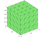
(a) Tetrahedral mesh

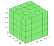
(b) Structured mesh

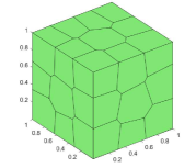
(c) CVT mesh

Fig. 29: Three types of discretizations

We solve the problem on three different kinds of meshes. One is the uniform triangulation shown in Fig. 29(a) and the others are the polyhedral meshes displayed in Fig. 29(b) and Fig. 29(c). The structured polyhedral mesh in Fig. 29(b) is formed by translating a two-dimensional polygonal mesh along the $z$-axis and connecting the corresponding vertices, hence all sides are quadrilaterals. The CVT meshes refer to the Centroidal Voronoi Tessellations, which are obtained from a set of seeds that coincide with barycenters of the resulting Voronoi cells. We generate such meshes via a standard Lloyd algorithm by extending the idea in the MATLAB toolbox - PolyMesher introduced in [45] to a cuboid.

Example 10.1.

Let $\alpha=1$. The right-hand side $f$ and the boundary conditions are chosen in such a way that the exact solution is

$$u(x,y,z)=\sin(2xy)\cos(z).$$

The results are displayed in Fig. 30, from which we observe that the optimal rates of convergence are achieved for all the three types of discretizations in the $H^{1}$ and $L^{2}$ norms. Note that the uniform triangulation is generated by cubemesh.m in $i$FEM.

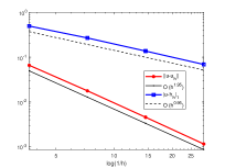
(a) Tetrahedral mesh

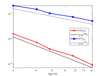
(b) Structured mesh

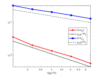
(c) CVT mesh

Fig. 30: Convergence rates in $L^{2}$ and $H^{1}$ norms for Example 10.1

Example 10.2.

In this example, the exact solution is chosen as

$$u(x,y,z)=\sin(\pi x)\cos(\pi y)\cos(\pi z).$$

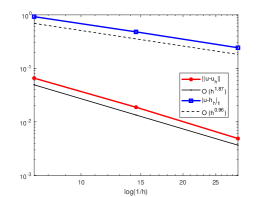
(a) Tetrahedral mesh

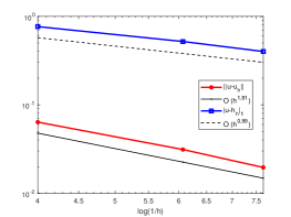
(b) Structured mesh

Fig. 31: Convergence rates in $L^{2}$ and $H^{1}$ norms for Example 10.2

Tab. 4: Discrete $L^{2}$ and $H^{1}$ errors of Example 10.2 for polyhedral meshes

$N$	$h$	ErrL2	ErrH1
170	2.500e-01	6.32804e-02	7.63490e-01
504	1.647e-01	3.09424e-02	5.18111e-01
1024	1.307e-01	1.94670e-02	4.00026e-01

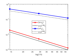
Fig. 32: Convergence rates in $L^{2}$ and $H^{1}$ norms of Example 10.2 for the triangulation with smaller mesh sizes

We still consider the problem with the Neumann boundary condition imposed on $x=0$ and repeat the numerical simulation in Example 10.1. The uniform triangulation is generated by cubemesh.m and further refined by uniformrefine3.m in $i$FEM. By default, the initial mesh before refining has mesh size $h=1$. We display the rate of convergence and the discrete errors in Fig. 31 and Tab. 4, respectively. It is evident that the code gives satisfactory accuracy and the optimal rate of convergence is achieved for the $H^{1}$ norm. However, the order of the error in the discrete $L^{2}$ norm is not close to 2. In fact, this phenomenon is also observed for the classical linear finite element methods under the same conditions. The reason lies in the coarse mesh. To get the optimal convergence rate, one can run the code on a sequence of meshes with much smaller sizes. For instance, Fig. 32 shows the result for the triangulation with initial size 0.25, in which case the optimal rates of convergence are obtained for both norms. It should be pointed out that the linear virtual element method on a triangulation is exactly the standard finite element method since in this case the virtual element space happens to be the set of polynomials of degree $k\leq 1$. Compared to the vectorized code in $i$FEM for the finite element methods, the current implementation is less efficient due to the large for loop. For example, three uniform refinements of the above initial triangulation will yield a mesh of 196608 triangular elements, and hence 196608 loops over the elements.

11 Concluding remarks

In this paper, a MATLAB software package for the virtual element method was presented for various typical problems. The usage of the library, named mVEM, was demonstrated through several examples. Possible extensions of this library that are of interest include time-dependent problems, adaptive mixed VEMs, three-dimensional linear elasticity, polyhedral mesh generator, and nonlinear solid mechanics. Various applications such as the Cahn-Hilliard problem, Stokes-Darcy problem and Navier-Stokes are also very appealing.

For three-dimensional problems, the current code can be further vectorized to achieve comparable performance in MATLAB with respect to compiled languages, where the most time-consuming part lies in the evaluation of the large number of face integrals and element integrals, for example, the elementwise computation of the $L^{2}$ projection matrices for the reaction-diffusion problems. To spare the computational cost, one may divide the polyhedral element as a union of some tetrahedrons and compute the integrals on those elements with the same number of tetrahedrons. Such a procedure can be vectorized in MATLAB with an additional effort of the code design. In the current version, we still do the elementwise loop as in [44] to make the code more transparent. mVEM is free and open source software.

References

- [1] D. Adak and S. Natarajan. Virtual element method for semilinear sine-Gordon equation over polygonal mesh using product approximation technique. Math. Comput. Simulation, 172:224–243, 2020.
- [2] B. Ahmad, A. Alsaedi, F. Brezzi, L. D. Marini, and A. Russo. Equivalent projectors for virtual element methods. Comput. Math. Appl., 66(3):376–391, 2013.
- [3] P. F. Antonietti, G. Manzini, and M. Verani. The fully nonconforming virtual element method for biharmonic problems. Math. Models Methods Appl. Sci., 28(2):387–407, 2018.
- [4] E. Artioli, L. Beirão da Veiga, C. Lovadina, and E. Sacco. Arbitrary order 2D virtual elements for polygonal meshes: part I, elastic problem. Comput. Mech., 60(3):355–377, 2017.
- [5] E. Artioli, L. Beirão da Veiga, C. Lovadina, and E. Sacco. Arbitrary order 2D virtual elements for polygonal meshes: part II, inelastic problem. Comput. Mech., 60(4):643–657, 2017.
- [6] B. Ayuso de Dios, K. Lipnikov, and G. Manzini. The nonconforming virtual element method. ESAIM Math. Model. Numer. Anal., 50(3):879–904, 2016.
- [7] L. Beirão da Veiga, F. Brezzi, A. Cangiani, G. Manzini, L. D. Marini, and A. Russo. Basic principles of virtual element methods. Math. Models Meth. Appl. Sci., 23(1):199–214, 2013.
- [8] L. Beirão da Veiga, F. Brezzi, A. Cangiani, G. Manzini, L. D. Marini, and A. Russo. Basic principles of mixed virtual element methods. ESAIM Math. Model. Numer. Anal., 48(4):1227–1240, 2014.
- [9] L. Beirão da Veiga, F. Brezzi, F. Dassi, L. D. Marini, and A. Russo. Serendipity virtual elements for general elliptic equations in three dimensions. Chinese Ann. Math. Ser. B, 39(2):315–334, 2018.
- [10] L. Beirão da Veiga, F. Brezzi, and L. D. Marini. Virtual elements for linear elasticity problems. SIAM J. Numer. Anal., 51(2):794–812, 2013.
- [11] L. Beirão da Veiga, F. Brezzi, L. D. Marini, and A. Russo. The hitchhiker’s guide to the virtual element method. Math. Models Meth. Appl. Sci., 24(8):1541–1573, 2014.
- [12] L. Beirão da Veiga, F. Brezzi, L. D. Marini, and A. Russo. Serendipity nodal VEM spaces. Comput. Fluids, 141:2–12, 2016.
- [13] L. Beirão da Veiga, F. Brezzi, L. D. Marini, and A. Russo. Virtual element implementation for general elliptic equations. In Building bridges: connections and challenges in modern approaches to numerical partial differential equations, volume 114 of Lect. Notes Comput. Sci. Eng., pages 39–71. Springer, [Cham], 2016.
- [14] L. Beirão da Veiga, F. Brezzi, L. D. Marini, and A. Russo. Virtual element method for general second-order elliptic problems on polygonal meshes. Math. Models Methods Appl. Sci., 26(4):729–750, 2016.
- [15] L. Beirão da Veiga, F. Dassi, and A. Russo. High-order virtual element method on polyhedral meshes. Comput. Math. Appl., 74(5):1110–1122, 2017.
- [16] L. Beirão Da Veiga, F. Dassi, and G. Vacca. The Stokes complex for virtual elements in three dimensions. Math. Models Methods Appl. Sci., 30(3):477–512, 2020.
- [17] L. Beirão da Veiga, C. Lovadina, and G. Vacca. Divergence free virtual elements for the Stokes problem on polygonal meshes. ESAIM Math. Model. Numer. Anal., 51(2):509–535, 2017.
- [18] L. Beirão da Veiga and G. Manzini. Residual a posteriori error estimation for the virtual element method for elliptic problems. ESAIM Math. Model. Numer. Anal., 49(2):577–599, 2015.
- [19] L. Beirão da Veiga, G. Manzini, and L. Mascotto. A posteriori error estimation and adaptivity in virtual elements. Numer. Math., 143(1):139–175, 2019.
- [20] S. Berrone and A. Borio. A residual a posteriori error estimate for the virtual element method. Math. Models Methods Appl. Sci., 27(8):1423–1458, 2017.
- [21] S. C. Brenner and L. R. Scott. The Mathematical Theory of Finite Element Methods. Springer, New York, 3rd edition, 2008.
- [22] F. Brezzi, R. S. Falk, and L. D. Marini. Basic principles of mixed virtual element methods. ESAIM Math. Model. Numer. Anal., 48(4):1227–1240, 2014.
- [23] F. Brezzi and L. D. Marini. Virtual element methods for plate bending problems. Comput. Methods Appl. Mech. Engrg., 253:455–462, 2013.
- [24] A. Cangiani, E. H. Georgoulis, T. Pryer, and O. J. Sutton. A posteriori error estimates for the virtual element method. Numer. Math., 137(4):857–893, 2017.
- [25] A. Cangiani, G. Manzini, and O. J. Sutton. Conforming and nonconforming virtual element methods for elliptic problems. IMA J. Numer. Anal., 37(3):1317–1354, 2017.
- [26] L. Chen. iFEM: an integrated finite element method package in MATLAB. Technical report, University of California at Irvine, 2009.
- [27] L. Chen and X. Huang. Nonconforming virtual element method for -th order partial differential equations in . Math. Comput., 89(324):1711–1744, 2020.
- [28] H. Chi, L. Beirão da Veiga, and G. H. Paulino. Some basic formulations of the virtual element method (VEM) for finite deformations. Comput. Methods Appl. Mech. Engrg., 318:148–192, 2017.
- [29] H. Chi, L. Beirão da Veiga, and G. H. Paulino. A simple and effective gradient recovery scheme and a posteriori error estimator for the virtual element method (vem). Comput. Methods Appl. Mech. Engrg., 347:21–58, 2019.
- [30] C. Chinosi and L. D. Marini. Virtual element method for fourth order problems: -estimates. Comput. Math. Appl., 72(8):1959–1967, 2016.
- [31] M. Cihan, B. Hudobivnik, F. Aldakheel, and P. Wriggers. 3D mixed virtual element formulation for dynamic elasto-plastic analysis. Comput. Mech., 68(3):581–598, 2021.
- [32] R. S. Falk. Nonconforming finite element methods for the equations of linear elasticity. Math. Comp., 57(196):529–550, 1991.
- [33] K. Feng and Z. Shi. Mathematical Theory of Elastic Structures. Springer-Verlag, Berlin, 1996.
- [34] A. Gain, G. Paulino, S. Leonardo, and I. Menezes. Topology optimization using polytopes. Comput. Methods Appl. Mech. Engrg., 293:411–430, 2015.
- [35] A. L. Gain, C. Talischi, and G. H. Paulino. On the virtual element method for three-dimensional linear elasticity problems on arbitrary polyhedral meshes. Comput. Methods Appl. Mech. Engrg., 282:132–160, 2014.
- [36] J. Huang and S. Lin. A time-stepping virtual element method for linear wave equations on polygonal meshes. Electron. Res. Arch., 28(2):911–933, 2020.
- [37] J. Huang and S. Lin. A posteriori error analysis of a non-consistent virtual element method for reaction diffusion equations. Appl. Math. Lett., 122:Paper No. 107531, 10, 2021.
- [38] J. Huang, S. Lin, and Y. Yu. A novel locking-free virtual element method for linear elasticity problems. arXiv:2112.13848, 2021.
- [39] X. Huang. Nonconforming virtual element method for 2th order partial differential equations in with . Calcolo, 57(4):42, 2020.
- [40] R. Kouhia and R. Stenberg. A linear nonconforming finite element method for nearly incompressible elasticity and Stokes flow. Comput. Methods Appl. Mech. Engrg., 124(3):195–212, 1995.
- [41] D. Y. Kwak and H. Park. Lowest-order virtual element methods for linear elasticity problems. Comput. Methods Appl. Mech. Engrg., 390:Paper No. 114448, 2022.
- [42] A. Ortiz-Bernardin, C. Alvarez, N. Hitschfeld-Kahler, A. Russo, R. Silva-Valenzuela, and E. Olate-Sanzana. Veamy: an extensible object-oriented C++ library for the virtual element method. Numer. Algorithms, 82:1189–1220, 2019.
- [43] K. Park, H. Chi, and G. H. Paulino. Numerical recipes for elastodynamic virtual element methods with explicit time integration. Internat. J. Numer. Methods Engrg., 121(1):1–31, 2020.
- [44] O. J. Sutton. The virtual element method in 50 lines of MATLAB. Numer. Algorithms, 75(4):1141–1159, 2017.
- [45] C. Talischi, G. H. Paulino, A. Pereira, and I. F. M. Menezes. Polymesher: a general-purpose mesh generator for polygonal elements written in Matlab. Struct. Multidiscip. Optim., 45(3):309–328, 2012.
- [46] G. Vacca. Virtual element methods for hyperbolic problems on polygonal meshes. Comput. Math. Appl., 74(5):882–898, 2017.
- [47] G. Vacca and L. Beirão da Veiga. Virtual element methods for parabolic problems on polygonal meshes. Numer. Methods Partial Differential Equations, 31(6):2110–2134, 2015.
- [48] F. Wang and H. Wei. Virtual element method for simplified friction problem. Appl. Math. Lett., 85:125–131, 2018.
- [49] F. Wang, B. Wu, and W. Han. The virtual element method for general elliptic hemivariational inequalities. J. Comput. Appl. Math., 389:Paper No. 113330, 19, 2021.
- [50] F. Wang and J. Zhao. Conforming and nonconforming virtual element methods for a Kirchhoff plate contact problem. IMA J. Numer. Anal., 41(2):1496–1521, 2021.
- [51] B. Wu, F. Wang, and W. Han. Virtual element method for a frictional contact problem with normal compliance. Commun. Nonlinear Sci. Numer. Simul., 107:Paper No. 106125, 13 pp., 2022.
- [52] Y. Yu. Implementation of polygonal mesh refinement in MATLAB. arXiv:2101.03456, 2021.
- [53] Y. Yu. A lowest-order locking-free nonconforming virtual element method based on the reduced integration technique for linear elasticity problems. arXiv:2112.13378v2, 2021.
- [54] B. Zhang, J. Zhao, Y. Yang, and S. Chen. The nonconforming virtual element method for elasticity problems. J. Comput. Phys., 378:394–410, 2019.
- [55] J. Zhao, S. Chen, and B. Zhang. The nonconforming virtual element method for plate bending problems. Math. Models Methods Appl. Sci., 26(9):1671–1687, 2016.
- [56] J. Zhao, B. Zhang, S. Chen, and S. Mao. The Morley-type virtual element for plate bending problems. J. Sci. Comput., 76(1):610–629, 2018.
- [57] J. Zhao, B. Zhang, S. Mao, and S. Chen. The divergence-free nonconforming virtual element for the Stokes problem. SIAM J. Numer. Anal., 57(6):2730–2759, 2019.