On a Bellman function associated with
the Chang–Wilson–Wolff theorem:
a case study

Abstract.

In this paper we estimate the tail of distribution (i. e., the measure of the set $\{f\geqslant x\}$) for those functions $f$ whose dyadic square function is bounded by a given constant. In particular we get a bit better estimate than the estimate following from the Chang–Wilson–Wolf theorem. In the paper we investigate the Bellman function corresponding to the problem. A curious structure of this function is found: it has jumps of the first derivative at a dense subset of interval $[0,1]$ (where it is calculated exactly), but it is of $C^{\infty}$-class for $x>\sqrt{3}$ (where it is calculated up to a multiplicative constant).

An unusual feature of the paper consists in the usage of computer calculations in the proof. Nevertheless, all the proofs are quite rigorous, since only the integer arithmetic was assigned to computer.

0. Level 0: What to keep in mind when reading this paper

0.1. Organization of the paper

Since this paper is quite technical in some places, we decided to write the text not in the usual “linear” manner where each statement is immediately followed by its proof and each proof contains all the needed auxiliary statements but rather in a “tree-like” manner where the top level is occupied by just the statements of the main results, the second level is occupied by the statements of the auxiliary results and the proofs of the main results without some technical details, the third level is occupied by the technical details missing in the second level and so on until we reach the last fifth level, which contains the proof of some specific numerical inequality needed before. So, the reader who wants only to get a general impression of what has been done in this article can read just Level 1; the reader who wants, in addition, to get a general idea of how everything is proved can stop reading at Level 2, and so on.

Such a structure means that at each level we will freely use the results from the next levels and the notation from the previous ones. Within each level we do employ the usual linear structure.

0.2. Warning about computer assisted proofs

Many of our proofs of various “elementary inequalities” are computer assisted. On the other hand, our standards for using computers in the proofs are quite strict: we allow only algebraic symbolic manipulation of rational functions and basic integer arithmetic. All our computations were done using the Mathematica program by Wolfram Research run on the Windows XP platform. We believe that there were no bugs in the software that could affect our results but, of course, the reader is welcome to check the computations using different programs on different platforms.

0.3. Notation and facts to remember throughout the entire text

The following facts and notation are “global” and will be used freely throughout the text without any further references after their first occurence. Everything else is “local” to each particular (sub)section and can be safely forgotten when exiting the corresponding (sub)section.

• The definition of the Haar functions $h_{{}_{\scriptstyle J}}$ (see Level 1);

• The definition of the square function $Sf$ (see Level 1);

• The definition and the properties of the non-linear mean $M$ (see Section 2.1.1);

• The definition and the properties of the dyadic suspension bridge $\mathcal{A}$ (see Section 2.1.2);

• The definition of the function $\mathcal{B}$ (see Level 1);

• The notation $X(x,\tau)=\dfrac{x+\tau}{\sqrt{1-\tau^{2}}}$;

• The Bellman inequality in its standard form (1) on page 1 and the inverse function form ($\ast \ast$ ‣ 2.5) on page $\ast \ast$ ‣ 2.5;

• The notation $\widetilde{\mathcal{B}}(x)=\left\{\begin{aligned} 1,&\quad x\leqslant 0;\\ \tfrac{1}{1+x^{2}},&\quad x\geqslant 0\end{aligned}\right.$ and the fact that $\widetilde{\mathcal{B}}$ satisfies the Bellman inequality;

• The definition of a supersolution and the fact that $\mathcal{B}$ is the least supersolution (Section 2.3);

• The notation $\Phi(x)=\int_{x}^{\infty}e^{-y^{2}/2}\,dy$ and $\Psi=\Phi^{-1}$;

• The differential Bellman inequality $xB^{\prime}(x)+B^{\prime\prime}(x)\leqslant 0$ and its equivalence to the concavity of the function $B\circ\Psi$ (Section 2.4);

• The increasing property of the ratio $\dfrac{\mathcal{B}(x)}{\Phi(x)}$ (Section 2.4).

This list is here to serve as a reminder to a reader who might otherwise occasionally get lost in this text or who might want to read its various parts in some non-trivial order. In addition to this list, it may be useful to keep in mind the statements in the titles of subsections and the summary of results in Level 1 though it is not formally necessary.

1. Level 1: Setup and main results

The celebrated Chang–Wilson–Wolff theorem ([1]) states that, if the square function of a function $f$ is uniformly bounded, then $e^{a|f|^{2}}$ is (locally) integrable for some positive $a$, which, in its turn, implies that the distribution tails $\mu\{f\geqslant x\}$ decay like $e^{-ax^{2}}$ where $\mu$ is the usual Lebesgue measure restricted to some interval. This theorem holds true for both discrete and continuous versions of the square function. The main aim of this article is to get sharp bounds for the distribution tails in the dyadic setting.

So, let $I=[0,1]$. Let $\mathcal{D}$ be the collection of all dyadic subintervals of the interval $I$. With each dyadic interval $J\in\mathcal{D}$, we will associate the corresponding Haar function $h_{{}_{\scriptstyle J}}$, which equals $-1$ on the left half $J_{-}$ of the interval $J$, equals $+1$ on its right half $J_{+}$, and equals $0$ outside the interval $J$.

Let now $f\colon I\to\mathbb{R}$ be any integrable function on $I$ such that $\int_{I}f=0$. Then $f=\sum_{J\in\mathcal{D}}a_{{}_{\scriptstyle J}}h_{{}_{\scriptstyle J}}$ where the coefficients $a_{{}_{\scriptstyle J}}$ can be found from the formula $a_{{}_{\scriptstyle J}}=\mu(J)^{-1}\int_{I}fh_{{}_{\scriptstyle J}}$ and the series converges both in $L^{1}$ and almost everywhere. The dyadic square function $Sf$ of the function $f$ is then defined by the formula

$$Sf=\sqrt{\sum_{J\in\mathcal{D}}a_{{}_{\scriptstyle J}}^{2}\chi_{{}_{\scriptstyle J}}}$$

where $\chi_{{}_{\scriptstyle J}}=h_{{}_{\scriptstyle J}}^{2}$ is the characteristic function of the dyadic interval $J$. The quantity we want to investigate is

$$\mathcal{B}(x)=\sup\{\mu\{f\geqslant x\}\colon\|Sf\|_{{}_{\scriptstyle L^{\infty}}}\leqslant 1\}\,,\qquad x\in\mathbb{R}\,.$$

Here is the summary of what we know and will prove in this article about the function $\mathcal{B}(x)$:

• $\mathcal{B}$ is a continuous non-increasing function on $\mathbb{R}$;

• $\mathcal{B}(x)=1$ for all $x\leqslant 0$ and $\mathcal{B}$ is strictly decreasing on $[0,+\infty)$;

• $\mathcal{B}(x)=1-\mathcal{A}^{-1}(x)$ for all $x\in[0,1]$ where $\mathcal{A}\colon[0,\frac{1}{2}]\to[0,1]$ is the “dyadic suspension bridge function” constructed in the beginning of Level 2;

• If $x\in[0,1]$ and $\mathcal{B}(x)$ is a binary rational number (i. e., a number of the kind $\frac{k}{2^{n}}$ with some non-negative integer $k$ and $n$), then we can explicitly construct a finite linear combination $f$ of Haar functions for which $\mu\{f\geqslant x\}=\mathcal{B}(x)$;

• There exists a positive constant $c$ (whose exact value remains unknown to us) such that $\mathcal{B}(x)=c\Phi(x)$ for all $x\geqslant\sqrt{3}$ where $\Phi$ is the Gaussian “error function”, i. e., $\displaystyle\Phi(x)=\int_{x}^{\infty}\!\!e^{-y^{2}/2}\,dy$.

Shortly put, this means that we know $\mathcal{B}$ exactly for $x\leqslant 1$, know it up to an absolute constant factor for $x\geqslant\sqrt{3}$ and do not have any clear idea about what $\mathcal{B}$ may be between $1$ and $\sqrt{3}$.

2. Level 2: Definitions, auxiliary results, and ideas of the proofs

2.1. Construction of the dyadic suspension bridge function $\mathcal{A}$

2.1.1. Nonlinear mean $M$

For any two real numbers $a,b$, we define their nonlinear mean $M[a,b]$ by

$$M[a,b]=\frac{a+b}{\sqrt{4+(a-b)^{2}}}\,.$$

The nonlinear mean $M[a,b]$ has the following properties.

1. $M[a,a]=a$;

2. $M[a,b]=M[b,a]$;

3. $M[a,b]\leqslant\dfrac{a+b}{2}$ for all $a,b\geqslant 0$;

4. $$\frac{\partial}{\partial a}M[a,b]=\frac{4+2b^{2}-2ab}{[4+(a-b)^{2}]^{3/2}}\,;$$

   When $a,b\in[0,1]$, the right hand side is strictly positive and does not exceed $\frac{6}{8}=\frac{3}{4}$ (the numerator is at most $6$ and the denominator is at least $8$). It follows immediately from here that

5. $M[a,b]$ is strictly increasing in each variable in the square $[0,1]^{2}$ and $M[a,b]$ lies strictly between $M[a,a]=a$ and $M[b,b]=b$ if $a,b\in[0,1]$ and $a\neq b$;

6. $|M[a,b]-a|\leqslant\frac{3}{4}|a-b|$ for all $a,b\in[0,1]$.

2.1.2. Definition of $\mathcal{A}$

Let

$$D_{n}=\left\{\frac{k}{2^{n}}\colon k=0,1,\dots,2^{n-1}\right\},\qquad n=1,2,3,\dots\,.$$

For any $t\in D_{n}\setminus D_{n-1}$ with $n\geqslant 2$, we define $t^{\pm}=t\pm 2^{-n}\in D_{n-1}$. Let $D=\bigcup_{n\geqslant 1}D_{n}$ be the set of all binary rational numbers on the interval $[0,\frac{1}{2}]$. We shall define the function $\mathcal{A}\colon D\to[0,1]$ as follows. Put $\mathcal{A}(0)=0$, $\mathcal{A}(\frac{1}{2})=1$. This completely defines $\mathcal{A}$ on $D_{1}$. Assume now that we already know the values of $\mathcal{A}$ on $D_{n-1}$. For each $t\in D_{n}\setminus D_{n-1}$, we put

$$\mathcal{A}(t)=M[\mathcal{A}(t^{-}),\mathcal{A}(t^{+})]\,.$$

This defines $\mathcal{A}$ inductively on the entire $D$. The first few steps of this construction look as follows:

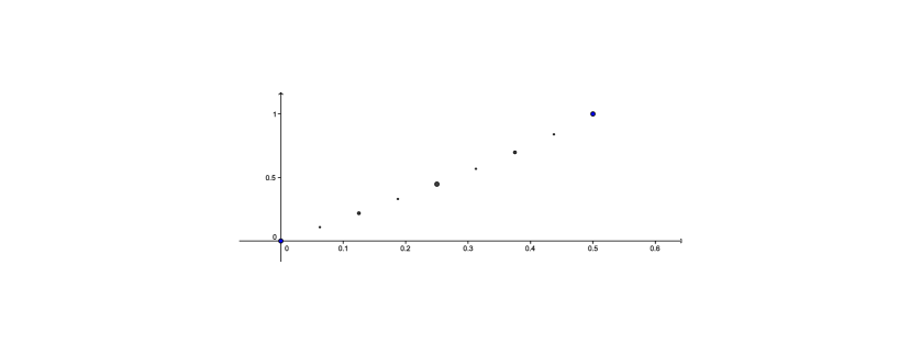
Figure 1. First steps in definition of $\mathcal{A}$.

After completing this procedure our function $\mathcal{B}(x)=1-\mathcal{A}^{-1}(x)$ will look like it is shown on Fig. 2.

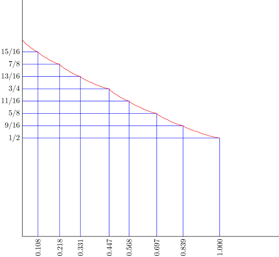
Figure 2. The graph of the function $\mathcal{B}=1-\mathcal{A}^{-1}$ on $[0,1]$.

Property (6) of the nonlinear mean $M$ implies that the difference of values of $\mathcal{A}$ at any two neighboring points of $D_{n}$ does not exceed $\left(\frac{3}{4}\right)^{n-1}$. It is not hard to derive from here that $\mathcal{A}$ is uniformly continuous on $D$ and, moreover, $\mathcal{A}\in\operatorname{Lip}_{\alpha}$ with $\alpha=\log_{2}\frac{4}{3}$. Thus, $\mathcal{A}$ can be extended continuously to the entire interval $[0,\frac{1}{2}]$. Property (5) implies that $\mathcal{A}$ is strictly increasing on $D$ and, thereby, on $[0,\frac{1}{2}]$. Thus, the inverse function $\mathcal{A}^{-1}\colon[0,1]\to[0,\frac{1}{2}]$ is well-defined and strictly increasing.

2.1.3. Properties of $\mathcal{A}$

The main properties of $\mathcal{A}$ we shall need is the estimate

$$\mathcal{A}(t)\leqslant 2t\qquad\text{ for all }t\in[0,\tfrac{1}{2}]\,,$$

the inequality

$$\mathcal{A}\left(\frac{s+t}{2}\right)\geqslant M[\mathcal{A}(s),\mathcal{A}(t)]\quad\text{ for all }s,t\in[0,\tfrac{1}{2}]\,,$$

and the fact that the function $\dfrac{\mathcal{A}(t)}{t}$ is non-decreasing on $(0,\frac{1}{2}]$. The first statement immediately follows from Property (3) of the nonlinear mean $M[a,b]$ by induction: at the points $t=0$ and $t=1$ we have $\mathcal{A}(t)=2t$, and if the inequality holds on $D_{n-1}$, then for $t\in D_{n}\setminus D_{n-1}$ we can estimate

$$\mathcal{A}(t)=M[\mathcal{A}(t^{-}),\mathcal{A}(t^{+})]\leqslant\frac{\mathcal{A}(t^{-})+\mathcal{A}(t^{+})}{2}\leqslant t^{-}+t^{+}=2t\,.$$

Thus, the assertion is true on $D$ and by continuity on the whole $[0,\tfrac{1}{2}]$. The proofs of two other statements can be found on Level 3 in Sections 3.2 and 3.3.

2.2. Continuity of $\mathcal{B}$

By definition, $\mathcal{B}$ is non-increasing on $\mathbb{R}$ and $\mathcal{B}(x)\geqslant 0$ for all $x\in\mathbb{R}$. It is easy to see that $\mathcal{B}(x)=1$ for $x\leqslant 0$ (just consider the identically zero test-function $f$). Let now $x\geqslant 0$. Take any test-function $f$ satisfying $\int_{I}f=0$ and $\|Sf\|_{{}_{\scriptstyle L^{\infty}}}\leqslant 1$. Construct a new function $g=g_{m,\delta}$ in the following way. Take an integer $m\geqslant 1$. Choose some $\delta\in(0,2^{-3m})$. Let $I_{j}=[0,2^{-j}]$, $J_{j}=(I_{j})_{+}=[2^{-(j+1)},2^{-j}]$ ($j=0,1,2,\dots$). Let $T_{j}$ be the linear mapping that maps $J_{j}$ onto $I$ (so, $T_{0}(x)=2x-1$, $T_{1}(x)=4x-1$, $T_{2}(x)=8x-1$, and so on). Put $f_{j}=f\circ T_{j}$ on $J_{j}$ and $f_{j}=0$ on $I\setminus J_{j}$. Now, let

$$g(x)=\delta\sum_{j=0}^{m-1}2^{j}h_{{}_{\scriptstyle I_{j}}}+\sqrt{1-2^{2m}\delta^{2}}\sum_{j=0}^{m}f_{j}\,.$$

The first sum may look a bit strange as written but it is just the Haar decomposition of the function $\left\{\begin{aligned} 1,\quad&\quad 2^{-m}\leqslant x\leqslant 1;\\ 1-2^{m},&\quad 0\leqslant x<2^{-m}\end{aligned}\right.$ multiplied by $\delta$ (cf. Fig. 3).

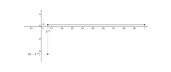
Figure 3. First summand of $g$.

Then, clearly, $\int_{I}g=0$. Since $f_{j}$ have mean $0$, are supported by disjoint dyadic intervals, and none of the functions $f_{j}$ from the second sum contains any of the function $h_{{}_{\scriptstyle I_{k}}}$ from the first sum in its Haar decomposition, we have

$$(Sg)^{2}\leqslant 1-2^{2m}\delta^{2}+\delta^{2}\sum_{j=0}^{m-1}2^{2j}\leqslant 1$$

on $I$. Finally, for each $j=0,1,\dots,m-1$, we have

$$\mu(\{g\geqslant\delta+\sqrt{1-2^{2m}\delta^{2}}\,x\}\cap J_{j})\geqslant\mu(\{f_{j}\geqslant x\}\cap J_{j})=2^{-(j+1)}\mu\{f\geqslant x\}$$

and, thereby, for the entire interval $I$, we have the inequality

$$\mu\{g\geqslant\delta+\sqrt{1-2^{2m}\delta^{2}}\,x\}\geqslant(1-2^{-m})\mu\{f\geqslant x\}\,.$$

Now, let us fix an integer $m>0$, thtn for every $x\in[0,2^{m-1}]$ and $\delta\in[0,2^{-3m}]$, we have

$$\delta+\sqrt{1-2^{2m}\delta^{2}}\,x\geqslant\delta+(1-2^{2m}\delta^{2})x=x+\delta(1-2^{2m}\delta x)\geqslant x+\frac{\delta}{2}\,.$$

Hence, by the definition of $\mathcal{B}$, we can write down the following estimate

$$\mathcal{B}\left(x+\tfrac{\delta}{2}\right)\geqslant\mu\{g\geqslant x+\tfrac{\delta}{2}\}\geqslant(1-2^{-m})\mu\{f\geqslant x\}\,.$$

Taking the supremum over all test-functions $f$ on the right hand side, we get

$$\mathcal{B}\left(x+\tfrac{\delta}{2}\right)\geqslant(1-2^{-m})\mathcal{B}(x)\,.$$

Recalling that $\mathcal{B}$ is non-increasing and $0\leqslant\mathcal{B}\leqslant 1$, we conclude from here that

$$0\leqslant\mathcal{B}(x)-\mathcal{B}\left(x+\tfrac{\delta}{2}\right)\leqslant 2^{-m}\,,$$

which immediately implies the uniform continuity of $\mathcal{B}$ on any compact subset of $\mathbb{R}$.

One useful corollary of this continuity result is the possibility to restrict ourselves to the functions $f$ that are finite linear combinations of the Haar functions in the definition of $\mathcal{B}$. Indeed, let $x\in\mathbb{R}$. Take any $\varepsilon>0$. Choose $x^{\prime}>x$ in such way that $\mathcal{B}(x^{\prime})\geqslant\mathcal{B}(x)-\varepsilon$. Choose a function $f$ satisfying $\int_{I}f=0$ and $\|Sf\|_{{}_{\scriptstyle L^{\infty}}}\leqslant 1$ such that $\mu\{f\geqslant x^{\prime}\}\geqslant\mathcal{B}(x^{\prime})-\varepsilon$. Let $f_{n}$ be the partial sums of the Haar series for $f$. Clearly, $\int_{I}f_{n}=0$ and $Sf_{n}\leqslant Sf$ everywhere on $I$. Since $f_{n}$ converge to $f$ almost everywhere on $I$, we can choose $n$ such that $\mu\{f_{n}\geqslant x\}\geqslant\mu\{f\geqslant x^{\prime}\}-\varepsilon$. But then $\mu\{f_{n}\geqslant x\}\geqslant\mathcal{B}(x)-3\varepsilon$. Moreover, considering the functions $g_{n}=(1-\frac{1}{n})f_{n}$ instead of $f_{n}$, we see that the supremum can be taken over finite linear combinations $f$ satisfying the strict inequality $\|Sf\|_{{}_{\scriptstyle L^{\infty}}}<1$.

2.3. The Bellman inequality

Take any $\tau\in(-1,1)$ and any two functions $f_{-},f_{+}\colon I\to\mathbb{R}$ satisfying $\int_{I}f_{\pm}=0$ and $\|Sf_{\pm}\|_{{}_{\scriptstyle L^{\infty}}}\leqslant 1$. Consider the function $f$ defined by

$$f(x)=\tau h_{{}_{\scriptstyle I}}+\sqrt{1-\tau^{2}}\begin{cases}f_{-}(2x),&0\leqslant x<\frac{1}{2}\,;\\ f_{+}(2x-1),&\frac{1}{2}\leqslant x\leqslant 1\,.\end{cases}$$

It is easy to see that $\int_{I}f=0$. Also, we have

$$((Sf)(x))^{2}=\tau^{2}+(1-\tau^{2})\begin{cases}((Sf_{-})(2x))^{2},&0\leqslant x<\frac{1}{2}\,;\\ ((Sf_{+})(2x-1))^{2},&\frac{1}{2}\leqslant x\leqslant 1\,,\end{cases}$$

whence $\|Sf\|_{{}_{\scriptstyle L^{\infty}}}\leqslant 1$. Now, it immediately follows from our definition of $f$ that, for every $x\in\mathbb{R}$,

$$\mu\{f\geqslant x\}=\frac{1}{2}\left[\mu\left\{f_{-}\geqslant\frac{x+\tau}{\sqrt{1-\tau^{2}}}\right\}+\mu\left\{f_{+}\geqslant\frac{x-\tau}{\sqrt{1-\tau^{2}}}\right\}\right]\,.$$

But, according to the definition of $\mathcal{B}$, the right hand side can be made as close to $\frac{1}{2}\left[\mathcal{B}\left(\frac{x+\tau}{\sqrt{1-\tau^{2}}}\right)+\mathcal{B}\left(\frac{x-\tau}{\sqrt{1-\tau^{2}}}\right)\right]$ as we wish by choosing appropriate $f_{\pm}$. Since our function $f$ belongs to the class of functions over which the supremum in the definition of $\mathcal{B}(x)$ is taken, we conclude that

(1) $$\mathcal{B}(x)\geqslant\frac{1}{2}\left[\mathcal{B}\left(\frac{x+\tau}{\sqrt{1-\tau^{2}}}\right)+\mathcal{B}\left(\frac{x-\tau}{\sqrt{1-\tau^{2}}}\right)\right]\,.$$

From now on, we shall use the notation $X(x,\tau)$ for $\frac{x+\tau}{\sqrt{1-\tau^{2}}}$. The inequality (1) will be referred to as the Bellman inequality from now on.

We shall call every non-increasing non-negative continuous function $B$ satisfying the Bellman inequality and the condition $B(x)=1$ for $x\leqslant 0$ a supersolution. Our next claim is that $\mathcal{B}$ is just the least supersolution. Since $\mathcal{B}$ is a supersolution, it suffices to show that $\mathcal{B}(x)\leqslant B(x)$ for any other supersolution $B$. It suffices to show that for any finite linear combination $f$ of the Haar functions satisfying $\|Sf\|_{{}_{\scriptstyle L^{\infty}}}<1$, we have $\mu\{f\geqslant x\}\leqslant B(x)$ for all $x\in\mathbb{R}$. We shall prove this statement by induction on the highest level of the Haar functions in the decomposition of $f$ (the level of the Haar function $h_{{}_{\scriptstyle J}}$ is just the number $n$ such that $\mu(J)=2^{-n}$). If $f$ is identically $0$ then the desired inequality immediately follows from the definition of a supersolution. Assume that our inequality is proved for all linear combinations containing only Haar functions up to level $n-1$ and that $f$ contains only Haar functions up to level $n$. Let $\tau$ be the coefficient at $h_{{}_{\scriptstyle I}}$ in the decomposition of $f$. Note that we must have $|\tau|<1$ (otherwise $Sf\geqslant 1$ on $I$). Let $T_{\pm}$ be the linear mappings that map $I$ onto $I_{\pm}$. Put $f_{\pm}=(f\circ T_{\pm}\mp\tau)/\sqrt{1-\tau^{2}}$. The functions $f_{\pm}$ are also finite linear combinations of Haar functions but they contain only Haar functions up to level $n-1$ (if $n=0$, it means that $f_{\pm}$ are identically $0$). Also, it is not hard to check that $\|Sf_{\pm}\|_{{}_{\scriptstyle L^{\infty}}}<1$. Now, clearly,

$$\mu\{f\geqslant x\}\leqslant\frac{1}{2}\big{[}\mu\{f_{-}\geqslant X(x,-\tau)\}+\mu\{f_{+}\geqslant X(x,\tau)\}\big{]}\\ \leqslant\frac{1}{2}\big{[}B(X(x,-\tau))+B(X(x,\tau))\big{]}\leqslant B(x)$$

by the induction assumption and the Bellman inequality. We are done.

Now we shall characterize all triples $(x_{-},x,x_{+})$ of real numbers such that $x_{\pm}=X(x,\pm\tau)$ for some $\tau\in(-1,1)$. A straightforward computation shows that in such case we must have $x=M[x_{-},x_{+}]$ and, conversely, if $x=M[x_{-},x_{+}]$, we can take $\tau=\dfrac{x_{+}-x_{-}}{\sqrt{4+(x_{+}-x_{-})^{2}}}$ and check that $x_{\pm}=X(x,\pm\tau)$ for this particular $\tau$. Thus, the Bellman inequality can be restated in the form that one must have

$$B(x)\geqslant\frac{1}{2}[B(x_{-})+B(x_{+})]$$

for all triples $x_{-},x,x_{+}$ satisfying the relation $x=M[x_{-},x_{+}]$.

In conclusion of this section, we show that it suffices to check the Bellman inequality only in the case when all three numbers $x_{-},x,x_{+}$ are non-negative. Indeed, if $x\leqslant 0$, then $B(x)=\max_{\mathbb{R}}B$ for any non-increasing function $B$ such that $B(x)=1$ for all $x\leqslant 0$, and the Bellman inequality becomes trivial. If $x>0$ and, say, $x_{-}<0$ (note that the roles of $x_{-}$ and $x_{+}$ are completely symmetric), we must have $x_{-}=X(x,-\tau)$ with $\tau>x>0$. But then $X(x,\tau)>0$ and the Bellman inequality becomes stronger if we replace $\tau>x$ by $\tau=x$. Indeed, $B(X(x,-\tau))$ and $B(x)$ will stay the same while $B(X(x,\tau))$ will not decrease because $B$ is non-increasing. This remark allows us to forget about the negative semiaxis at all and to define a supersolution as a non-negative non-increasing continuous function defined on $[0,+\infty)$ and satisfying the Bellman inequality there together with the condition $B(0)=1$.

2.4. Smooth supersolutions and the differential Bellman inequality

Suppose now that a supersolution $B$ is twice continuously differentiable on $(0,+\infty)$. Then we have the Taylor expansion

$$B(X(x,\pm\tau))=B(x)\pm B^{\prime}(x)\tau+\frac{1}{2}(xB^{\prime}(x)+B^{\prime\prime}(x))\tau^{2}+o(\tau^{2})\quad\text{as }\tau\to 0\,.$$

Plugging this expansion into the Bellman inequality, we see that we must have

$$xB^{\prime}(x)+B^{\prime\prime}(x)\leqslant 0$$

for all $x>0$. It is not hard to solve the corresponding linear differential equation: one possible solution is

$$\Phi(x)=\int_{x}^{\infty}\!\!\!e^{-y^{2}/2}\,dy$$

and the general solution is $C_{1}\Phi+C_{2}$ where $C_{1},C_{2}$ are arbitrary constants.

Let $\Psi\colon(0,\Phi(-\infty))\to(-\infty,+\infty)$ be the inverse function to $\Phi$. By the inverse function theorem, we have

$$\Psi^{\prime}=\frac{1}{\Phi^{\prime}\circ\Psi}=-e^{\Psi^{2}/2}\,.$$

Hence,

$$(B\circ\Psi)^{\prime\prime}=e^{\Psi^{2}}((B^{\prime}\circ\Psi)\cdot\Psi+B^{\prime\prime}\circ\Psi)\,.$$

Therefore, the differential Bellman inequality is equivalent to concavity of $B\circ\Psi$ on $(0,\Psi(-\infty))$. Since for any non-negative concave function $G$ on $(0,\Phi(-\infty))$, the ratio $G(t)/t$ is non-increasing, we conclude that the ratio $\dfrac{B(\Psi(t))}{t}$ is non-increasing and, thereby, the ratio $\dfrac{B(x)}{\Phi(x)}$ is non-decreasing on $(-\infty,+\infty)$.

The last two conditions (the concavity of $B\circ\Psi$ and the non-decreasing property of the ratio $\dfrac{B(x)}{\Phi(x)}$) would make perfect sense for all supersolutions, whether smooth or not. So, it would be nice to show that every supersolution can be approximated by a $C^{2}$-smooth one with arbitrary precision. To do it, just note that for every $x_{-},x_{+}\in\mathbb{R}$ and every $y\geqslant 0$, we have

$$M[x_{-}-y,x_{+}-y]=M[x_{-},x_{+}]-\frac{2y}{\sqrt{4+(x_{+}-x_{-})^{2}}}\geqslant M[x_{-},x_{+}]-y\,.$$

This allows us to conclude that if $B$ is a supersolution, then so is $B(\,\cdot\,-y)$ for all $y\geqslant 0$. Also note that any convex combination of supersolutions is a supersolution as well. Now just take any non-negative $C^{2}$ function $\eta$ supported by $[0,1]$ with total integral $1$, for $\delta>0$, define $\eta_{\delta}(x)=\delta^{-1}\eta(\delta^{-1}x)$, and consider the convolutions $B_{\delta}=B*\eta_{\delta}$. On one hand, each $B_{\delta}$ is a supersolution. On the other hand, $B_{\delta}\to B$ pointwise as $\delta\to\infty$.

2.5. $\mathcal{B}$ is strictly decreasing on $[0,+\infty)$

Let us start with showing that $B(x)<1$ for all $x>0$. For this, it suffices to note that the inequality $\|Sf\|_{{}_{\scriptstyle L^{\infty}}}\leqslant 1$ implies

$$\int_{I}f^{2}=\int_{I}(Sf)^{2}\leqslant 1\,.$$

Now, if we consider the problem of maximizing $\mu\{f\geqslant x\}$ under the restrictions $\int_{I}f=0$ and $\int_{I}f^{2}\leqslant 1$, we shall get another function $\widetilde{\mathcal{B}}(x)$ on $[0,+\infty)$. Since we relaxed our restrictions, we must have $\mathcal{B}\leqslant\widetilde{\mathcal{B}}$ everywhere. But, unlike our original problem of finding $\mathcal{B}$, to find $\widetilde{\mathcal{B}}$ exactly is a piece of cake: we have

$$\widetilde{\mathcal{B}}(x)=\frac{1}{1+x^{2}}\qquad\text{ for all }x\geqslant 0\,.$$

The reader can try to prove this statement himself or to look up the proof on Level 3. Right away, we shall only mention that $\widetilde{\mathcal{B}}(t)$ satisfies the condition $\widetilde{\mathcal{B}}(0)=1$ and the same Bellman inequality (the derivation of which is almost exactly the same as before; actually, the only result in this section that is impossible to repeat for $\widetilde{\mathcal{B}}$ in place of $\mathcal{B}$ is to show that it is the least supersolution).

Now, when we know that $\mathcal{B}(x)\leqslant\frac{1}{1+x^{2}}<1$ for $x>0$, the strict monotonicity becomes relatively easy. Indeed, assume that $\mathcal{B}(x)=\mathcal{B}(y)=a$ for some $0<x<y$. Then $a<1$. Due to the continuity of $\mathcal{B}$, we can choose the least $x\geqslant 0$ satisfying $\mathcal{B}(x)=a$. This $x\neq 0$ because $\mathcal{B}(0)=1>a$, so we must have $x>0$. Also, we still have $x<y$. Take now $\tau>0$ so small that $X(x,-\tau)<x$ and $X(x,\tau)<y$. Then the Bellman inequality immediately implies that $\mathcal{B}(X(x,-\tau))\leqslant 2\mathcal{B}(x)-\mathcal{B}(X(x,\tau))\leqslant 2\mathcal{B}(x)-\mathcal{B}(y)=a$. Since we must also have $\mathcal{B}(X(x,-\tau))\geqslant\mathcal{B}(x)=a$, we obtain $\mathcal{B}(X(x,-\tau))=a$, which contradicts the minimality of $x$. It is worth mentioning that a similar argument can be used to derive continuity directly from the Bellman inequality. We leave the details to the reader.

The strict monotonicity property implies that $\mathcal{B}^{-1}$ is well defined. Also, since $\mathcal{B}(x)\leqslant\widetilde{\mathcal{B}}(x)$, we must have $\mathcal{B}(x)\to 0+$ as $x\to\infty$. Thus, $\mathcal{B}^{-1}$ continuously maps the interval $(0,1]$ onto $[0,+\infty)$. The Bellman inequality is equivalent to the statement that

$$x=\mathcal{B}^{-1}(\mathcal{B}(x))\leqslant\mathcal{B}^{-1}\left(\frac{\mathcal{B}(x_{-})+\mathcal{B}(x_{+})}{2}\right)$$

for all triples $x_{-},\,x,\,x_{+}$ of non-negative numbers such that $x=M[x_{-},x_{+}]$. Denoting $\mathcal{B}(x_{-})=s$, $\mathcal{B}(x_{+})=t$, we see that the last inequality is equivalent to

$\ast \ast$ $$\mathcal{B}^{-1}\left(\frac{s+t}{2}\right)\geqslant M[\mathcal{B}^{-1}(s),\mathcal{B}^{-1}(t)]\,.$$

2.6. $\mathcal{B}=c\Phi$ beyond $\sqrt{3}$

Our first task here will be to show that the function $\Phi$ satisfies the Bellman inequality (1) if $x\geqslant\sqrt{3}$. Note that the inequality is an identity when $\tau=0$. So it suffices to show that

$$\frac{\partial}{\partial\tau}[\Phi(X(x,-\tau)+\Phi(X(x,\tau))]\leqslant 0\qquad\text{ for all }\tau\in[0,1)\,,$$

which, after a few simple algebraic manipulations, reduces to the inequality

$$(1+x\tau)e^{-x\tau/(1-\tau^{2})}\geqslant(1-x\tau)e^{x\tau/(1-\tau^{2})}\,.$$

If $x\tau\geqslant 1$, the left hand side is non-negative and the right hand side is non-positive. If $x\tau<1$, we can rewrite the inequality to prove in the form

$$\frac{1}{2}\log\frac{1+x\tau}{1-x\tau}-\frac{x\tau}{1-\tau^{2}}\geqslant 0\,.$$

Expanding the left hand side into a Taylor series with respect to $\tau$, we obtain the inequality

$$\sum_{k\geqslant 0}x\left(\frac{x^{2k}}{2k+1}-1\right)\tau^{2k+1}\geqslant 0$$

to prove. Observe that the coefficient at $\tau$ is always $0$ and the coefficient at $\tau^{3}$ is negative if $0\leqslant x<\sqrt{3}$. It means that our inequality holds with the opposite sign for all sufficiently small $\tau$ if $0\leqslant x<\sqrt{3}$ and, thereby, the Bellman inequality fails for such $x$ and $\tau$ as well. On the other hand, if $x\geqslant\sqrt{3}$, then all the coefficients on the left hand side are non-negative and the inequality holds.

Now let $c=\mathcal{B}(\sqrt{3})/\Phi(\sqrt{3})$. Consider the function $B(x)$ defined by

$$B(x)=\left\{\begin{aligned} \mathcal{B}(x),&\quad x\leqslant\sqrt{3}\,;\\ c\Phi(x),&\quad x\geqslant\sqrt{3}\,.\end{aligned}\right.$$

Note that, since the ratio $\dfrac{\mathcal{B}(x)}{\Phi(x)}$ is non-decreasing, we actually have $B(x)=\min\{\mathcal{B}(x),c\Phi(x)\}$ everywhere on $\mathbb{R}$. Indeed, $\mathcal{B}(\sqrt{3})=c\Phi(\sqrt{3})$ by our choice of $c$, whence $\mathcal{B}\geqslant c\Phi$ on $[\sqrt{3},+\infty)$ and $\mathcal{B}\leqslant c\Phi$ on $(-\infty,\sqrt{3}]$. Clearly, $B(x)=\mathcal{B}(x)=1$ for $x\leqslant 0$, $B$ is non-negative, continuous, and non-increasing. Let us check the Bellman inequality for $B$. Take any triple $x_{-},\,x,\,x_{+}$ with $x=M[x_{-},x_{+}]$. If $x\leqslant\sqrt{3}$, we have

$$B(x)=\mathcal{B}(x)\geqslant\frac{1}{2}[\mathcal{B}(x_{-})+\mathcal{B}(x_{+})]\geqslant\frac{1}{2}[B(x_{-})+B(x_{+})]\,.$$

If $x\geqslant\sqrt{3}$, we have

$$B(x)=c\Phi(x)\geqslant\frac{1}{2}[c\Phi(x_{-})+c\Phi(x_{+})]\geqslant\frac{1}{2}[B(x_{-})+B(x_{+})]\,.$$

Thus, $B$ is a supersolution and, therefore, $\mathcal{B}\leqslant B$ everywhere. But we also know that $\mathcal{B}\geqslant B$ everywhere. Thus, $\mathcal{B}=B$, i. e., $\mathcal{B}=c\Phi$ on $[\sqrt{3},\infty)$.

2.7. $\mathcal{B}=1-\mathcal{A}^{-1}$ on $[0,1]$

The first observation to make here is that we know the value $\mathcal{B}(1)$ exactly: $\mathcal{B}(1)=\frac{1}{2}$. Indeed, the inequality $\mathcal{B}(1)\leqslant\frac{1}{2}$ follows from the estimate $\mathcal{B}(x)\leqslant\widetilde{\mathcal{B}}(x)=\frac{1}{1+x^{2}}$ and the inequality $\mathcal{B}(1)\geqslant\frac{1}{2}$ follows from the consideration of the test-function $f=h_{{}_{\scriptstyle I}}$. Consider now the function $G(t)=\mathcal{B}^{-1}(1-t)$. It is continuous, increasing and maps $[0,\frac{1}{2}]$ onto $[0,1]$. According to the Bellman inequality in the form ($\ast \ast$ ‣ 2.5), we must have

$$G\left(\frac{s+t}{2}\right)\geqslant M[G(s),G(t)]\qquad\text{ for all }s,t\in[0,\tfrac{1}{2}],.$$

Also $G(0)=0=\mathcal{A}(0)$ and $G(\frac{1}{2})=1=\mathcal{A}(\frac{1}{2})$. Since $M$ is monotone in each variable on $[0,1]^{2}$, we can easily prove by induction that $G\geqslant\mathcal{A}$ on $D$ and, therefore, by continuity, on $[0,\frac{1}{2}]$. Applying $\mathcal{B}$ to both sides of this inequality, we conclude that $1-t\leqslant\mathcal{B}(\mathcal{A}(t))$ on $[0,\frac{1}{2}]$. Taking $t=\mathcal{A}^{-1}(x)$ ($x\in[0,1]$), we, finally, get

$$\mathcal{B}(x)\geqslant 1-\mathcal{A}^{-1}(x)\qquad\text{ for all }x\in[0,1]\,.$$

It remains only to prove the reverse inequality. To this end, it would suffice to show that the function

$$B(x)=\begin{cases}1,&x\leqslant 0;\\ 1-\mathcal{A}^{-1}(x),&0\leqslant x\leqslant 1\,;\\ \frac{1}{1+x^{2}},&x\geqslant 1\,.\end{cases}$$

is a supersolution. The only non-trivial property to check is the Bellman inequality. It has been already mentioned above that we may restrict ourselves to the case when all three numbers $x_{-},x,x_{+}$ are non-negative. Consider all possible cases:

2.7.1. Case 1: all three numbers are on $[0,1]$

In this case, we can just check the Bellman inequality in the form ($\ast \ast$ ‣ 2.5), which reduces to the already mentioned inequality

$$\mathcal{A}\left(\frac{s+t}{2}\right)\geqslant M[\mathcal{A}(s),\mathcal{A}(t)]\quad\text{ for all }s,t\in[0,\frac{1}{2}]$$

whose proof can be found on Level 3.

2.7.2. Case 2: $x>1$

Here all we need is to note that, since $\mathcal{A}(t)\leqslant 2t$, we have

$$1-\mathcal{A}^{-1}(x)\leqslant 1-\frac{x}{2}\leqslant\frac{1}{1+x^{2}}=\widetilde{\mathcal{B}}(x)$$

on $[0,1]$. Therefore, we can use the fact that the Bellman inequality is true for $\widetilde{\mathcal{B}}$ and write

$$B(x)=\widetilde{\mathcal{B}}(x)\geqslant\frac{1}{2}[\widetilde{\mathcal{B}}(x_{-})+\widetilde{\mathcal{B}}(x_{+})]\geqslant\frac{1}{2}[B(x_{-})+B(x_{+})]\,.$$

2.7.3. Case 3: $0<x<1$, $x_{+}\geqslant 1$

We can always assume that it is $x_{+}$ that is greater than $1$ because the roles of $x_{+}$ and $x_{-}$ in the Bellman inequality are completely symmetric. Note that when $0<x<1$, we have

$$\frac{\partial}{\partial\tau}X(x,\tau)=\frac{1+x\tau}{(1-\tau^{2})^{3/2}}>0$$

for all $\tau\in(-1,1)$. Thus, if $x_{+}>x$, we must have $\tau>0$ and $x_{-}=X(x,-\tau)<x$. The condition $x_{-}\geqslant 0$ implies that $\tau\leqslant x$.

First we consider the boundary case when $x_{-}=0$. Then $x_{+}=X(x,x)=\frac{2x}{\sqrt{1-x^{2}}}$, which is greater than or equal to $1$ if and only if $x\geqslant\tfrac{1}{\sqrt{5}}$. Then the inequality we need to prove reduces to

$$B(x)\geqslant\frac{1}{2}\bigl{[}B(X(x,x))+1\bigr{]}=\frac{1+x^{2}}{1+3x^{2}}\,.$$

Denote that function $\frac{1+x^{2}}{1+3x^{2}}$ on the right hand side by $F(x)$ and note that at the endpoints of this interval we have the identities $B(\tfrac{1}{\sqrt{5}})=F(\tfrac{1}{\sqrt{5}})=\frac{3}{4}$ and $B(1)=F(1)=\frac{1}{2}$. Recall also that $B\circ\Psi$ is concave on $\Psi^{-1}([\tfrac{1}{\sqrt{5}},1])$ (formally we proved this only for supersolutions but, since only arbitrarily small values of $\tau$ were used in the proof, we can conclude that this concavity result also holds for any non-negative non-increasing continuous function $B$ satisfying the Bellman inequality just for the triples $x_{-},\,x,\,x_{+}$ contained in $[\tfrac{1}{\sqrt{5}},1]$). So, it would suffice to show that the function $F\circ\Psi$ is convex on the same interval, which is equivalent to the assertion that $xF^{\prime}(x)+F^{\prime\prime}(x)\geqslant 0$ on $[\tfrac{1}{\sqrt{5}},1]$. A direct computation yields

$$xF^{\prime}(x)+F^{\prime\prime}(x)=4\frac{8x^{2}-3x^{4}-1}{(1+3x^{2})^{3}}\,.$$

But

$$8x^{2}-3x^{4}-1=3x^{2}(1-x^{2})+(5x^{2}-1)\geqslant 0$$

on $[\tfrac{1}{\sqrt{5}},1]$ and we are done.

Now we are ready to handle the remaining case $0<x_{-}<x<1<x_{+}$. Let $\widetilde{x}_{+}=X(x,x)$ and let $\widetilde{x}_{-}=X(x,-\tau)$ where $\tau\in(0,1)$ is chosen in such a way that $X(x,\tau)=1$. Then $0<x_{-}<\widetilde{x}_{-}<x<1<x_{+}<\widetilde{x}_{+}$ and we have the Bellman inequality for the triples $0,\,x,\,\widetilde{x}_{+}$ and $\widetilde{x}_{-},\,x,\,1$. If

$$B(x_{+})-B(\widetilde{x}_{+})\leqslant B(0)-B(x_{-})\quad\text{ or }\quad B(x_{-})-B(\widetilde{x}_{-})\leqslant B(1)-B(x_{+})\,,$$

we can prove the desired Bellman inequality for the triple $x_{-},\,x,\,x_{+}$ by comparing it to the known Bellman inequality for the triple $0,\,x,\,\widetilde{x}_{+}$ or $\widetilde{x}_{-},\,x,\,1$ respectively. So, the only situation that is bad for us is the one when the strict inequalities

$$B(x_{+})-B(\widetilde{x}_{+})>B(0)-B(x_{-})\quad\text{and}\quad B(x_{-})-B(\widetilde{x}_{-})>B(1)-B(x_{+})$$

hold simultaneously. Now observe that, if four positive numbers $a,\,b,\,c,\,d$ satisfy $a>c$ and $b>d$, then we also have $\dfrac{c}{c+b}<\dfrac{a}{a+d}$. Thus, in the bad situation, we must have

$$\frac{B(0)-B(x_{-})}{B(0)-B(\widetilde{x}_{-})}<\frac{B(x_{+})-B(\widetilde{x}_{+})}{B(1)-B(\widetilde{x}_{+})}\,.$$

Since $\frac{\mathcal{A}(t)}{t}$ is non-decreasing on $[0,\frac{1}{2}]$, we can say that

$$\frac{B(0)-B(x_{-})}{B(0)-B(\widetilde{x}_{-})}\geqslant\frac{x_{-}}{\widetilde{x}_{-}}\,.$$

So, in the bad situation we must have the inequality

$$\frac{x_{-}}{\widetilde{x}_{-}}<\frac{B(x_{+})-B(\widetilde{x}_{+})}{B(1)-B(\widetilde{x}_{+})}\,.$$

Note that everywhere in this inequality the function $B(x)$ coincides with $\widetilde{\mathcal{B}}(x)=\frac{1}{1+x^{2}}$. So, this is an elementary inequality (it contains fractions and square roots, of course, but still it is a closed form inequality about functions given by explicit algebraic formulae). It turns out that exactly the opposite inequality is always true (the proof can be found on Level 4, Subsection 4.5), so we are done with this case too.

2.8. Optimal functions for binary rational values of $\mathcal{B}$

By the construction of the dyadic suspension bridge $\mathcal{A}$, for every point $t\in D\setminus\{0,\frac{1}{2}\}$, we have $\mathcal{A}(t)=M[\mathcal{A}(t_{-}),\mathcal{A}(t_{+})]$. Let now $x=\mathcal{A}(t)$ for some $t\in D$ and let $x_{-}=\mathcal{A}(t_{-})$, $x_{+}=\mathcal{A}(t_{+})$. Then for the triple $x_{-},\,x,\,x_{+}$, the Bellman inequality becomes an identity and we can say that if we have a pair $f_{\pm}$ of finite linear combinations of Haar functions such that $\|Sf_{\pm}\|_{{}_{\scriptstyle L^{\infty}}}\leqslant 1$ and $\mu\{f_{\mp}\geqslant x_{\pm}\}=\mathcal{B}(x_{\pm})$, then, if we take $\tau\in(0,1)$ such that $x_{\pm}=X(x,\pm\tau)$ and define $f$ by

$$f=\tau h_{{}_{\scriptstyle I}}+\sqrt{1-\tau^{2}}\begin{cases}f_{-}(2x),&0\leqslant x<\frac{1}{2}\,;\\ f_{+}(2x-1),&\frac{1}{2}\leqslant x\leqslant 1\,,\end{cases}$$

we shall get a finite linear combination of Haar functions satisfying $\|Sf\|_{{}_{\scriptstyle L^{\infty}}}\leqslant 1$ and $\mu\{f\geqslant x\}=\mathcal{B}(x)$. Since we, indeed, have such extremal linear combinations for $x=0$ and $x=1$ (the identically $0$ function and the function $h_{{}_{\scriptstyle I}}$ respectively), we can now recursively construct an extremal linear combination for any $x=\mathcal{A}(t)$ with $t\in D$. Take, for instance, $\mathcal{A}(\frac{3}{8})$. The construction of the extremal function for this value reduces to finding the coefficient $\tau=\dfrac{\mathcal{A}(\frac{1}{2})-\mathcal{A}(\frac{1}{4})}{\sqrt{4+(\mathcal{A}(\frac{1}{2})-\mathcal{A}(\frac{1}{4}))^{2}}}$ and two extremal functions: one for $\mathcal{A}(\frac{1}{4})$ and one for $\mathcal{A}(\frac{1}{2})$. The construction of the extremal function for $\mathcal{A}(\frac{1}{4})$ reduces to finding the coefficient $\tau=\dfrac{\mathcal{A}(\frac{1}{2})-\mathcal{A}(0)}{\sqrt{4+(\mathcal{A}(\frac{1}{2})-\mathcal{A}(0))^{2}}}$ and two more extremal functions: one for $\mathcal{A}(0)$ and one for $\mathcal{A}(\frac{1}{2})$. But we know that the extremal function for $\mathcal{A}(0)=0$ is $0$ and the extremal function for $\mathcal{A}(\frac{1}{2})=1$ is $h_{{}_{\scriptstyle I}}$. So, we can put everything together and get a linear combination of $4$ Haar functions that is extremal for $\mathcal{A}(\frac{3}{8})$. This construction is shown on the picture 4.

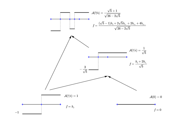
Figure 4. The construction of the extremal function for $\mathcal{A}(\frac{3}{8})$.

The resulting linear combination is

$$\frac{1}{\sqrt{26-2\sqrt{5}}}\left[(\sqrt{5}-1)h_{{}_{\scriptstyle I}}+2\sqrt{5}h_{{}_{\scriptstyle I_{-}}}+2h_{{}_{\scriptstyle I_{+}}}+4h_{{}_{\scriptstyle I_{+-}}}\right]\,,$$

which, indeed, equals $\mathcal{A}(\frac{3}{8})=\frac{\sqrt{5}+1}{\sqrt{26-2\sqrt{5}}}$ on the union $I_{-+}\cup I_{++}\cup I_{+-+}$ whose measure is exactly $\frac{5}{8}$. The square function, in its turn, equals $1$ on $I_{-}\cup I_{+-}$ and is strictly less than $1$ on $I_{++}$.

The simplest picture is obtained when we construct an extremal function for $\mathcal{A}(2^{-n})$. What we get is just the function

$$\sqrt{\frac{3}{4^{n}-1}}\Big{(}1-2^{n}\chi_{{}_{[0,2^{-n}]}}\Big{)}$$

that takes just two different values: one small positive on a big set and one large negative on a small set. The interested reader may amuse himself with drawing more pictures, trying to figure out how many Haar functions are needed to construct an extremal function for any particular “good” value of $x$, or proving that for all other values of $x\in[0,1]$ there are no extremal functions at all, but we shall stop here.

3. Level 3: Reductions to elementary inequalities

3.1. $\widetilde{\mathcal{B}}(x)=\frac{1}{1+x^{2}}$ for $x\geqslant 0$

Recall that

$$\widetilde{\mathcal{B}}(x)\buildrel\rm{def}\over{=}\sup\Bigl{\{}\mu\{f\geqslant x\}\colon\int_{I}f=0\,,\ \int_{I}f^{2}\leqslant 1\Bigr{\}}.$$

Considering the identically zero test-function $f$, we see that $\widetilde{\mathcal{B}}(x)=1$ fot all $x\leqslant 0$. Let now $x>0$. Putting

$$f(y)=\begin{cases}\displaystyle\ \ x,&\displaystyle 0\leqslant y\leqslant\frac{1}{1+x^{2}};\\ \displaystyle-\frac{1}{x},&\displaystyle\frac{1}{1+x^{2}}<y\leqslant 1\,,\end{cases}$$

we see that $\widetilde{\mathcal{B}}(x)\geqslant\frac{1}{1+x^{2}}$.

Now, take any test-function $f$. Let $E=\{f\geqslant x\}$ and let $m=\mu(E)$. Then

$$\int_{I\setminus E}f=-\int_{E}f\leqslant-mx$$

and

$$\int_{I\setminus E}f^{2}\geqslant\frac{1}{\mu(I\setminus E)}\Bigl{|}\int_{I\setminus E}f\Bigr{|}^{2}\geqslant\frac{m^{2}x^{2}}{1-m}$$

by Cauchy-Schwartz. Thus,

$$\int_{I}f^{2}=\int_{E}f^{2}+\int_{I\setminus E}f^{2}\geqslant mx^{2}+\frac{m^{2}x^{2}}{1-m}=\frac{m}{1-m}x^{2}\,.$$

Since this integral is bounded by $1$, we get the inequality

$$\frac{m}{1-m}x^{2}\leqslant 1\,,$$

whence $m\leqslant\dfrac{1}{1+x^{2}}$ .

One more thing we want to do in this section is to show directly that $\widetilde{\mathcal{B}}$ is a supersolution. If $x,X(x,\pm\tau)\geqslant 0$, the Bellman inequality

$$\widetilde{\mathcal{B}}(x)\geqslant\frac{1}{2}[\widetilde{\mathcal{B}}(X(x,-\tau)+\widetilde{\mathcal{B}}(X(x,\tau))]$$

reduces to

$$\frac{1}{1+x^{2}}\geqslant\frac{1}{2}\left[\frac{1-\tau^{2}}{1-2x\tau+x^{2}}+\frac{1-\tau^{2}}{1+2x\tau+x^{2}}\right]=\frac{(1-\tau^{2})(1+x^{2})}{(1+x^{2})^{2}-4x^{2}\tau^{2}}\,,$$

which is equivalent to

$$(1-\tau^{2})(1+x^{2})^{2}\leqslant(1+x^{2})^{2}-4x^{2}\tau^{2}\,.$$

Subtracting $(1+x^{2})^{2}$ from both sides, we get

$$(1+x^{2})^{2}\tau^{2}\geqslant 4x^{2}\tau^{2}\,.$$

Reducing by $\tau^{2}$ and taking the square root of both sides, we get the inequality

$$1+x^{2}\geqslant 2x\,,$$

which is obviously true.

3.2. The inequality $\mathcal{A}(\tfrac{s+t}{2})\geqslant M[A(s),A(t)]$

Since $\mathcal{A}$ is continuous, it suffices to check this inequality for $s,t\in D$. If $s,t\in D_{1}$, then our inequality turns into an identity. Suppose now that we already know that our inequality holds for all $s,t\in D_{n-1}$. To check its validity on $D_{n}$, we have to consider $2$ cases:

3.2.1. Case 1: $s\in D_{n}\setminus D_{n-1},t\in D_{n-1}$

Let $s^{\pm}=s\pm 2^{-n}$. Note that $s^{-}$ and $s^{+}$ are two neighboring points in $D_{n-1}$, whence they must lie on the same side of $t$ (it is possible that one of them coincides with $t$). Denote $y=\mathcal{A}(s^{-})$, $z=\mathcal{A}(s^{+})$. By the definition of the dyadic suspension bridge function $\mathcal{A}$, we then have

$$\mathcal{A}(s)=M[y,z]\,.$$

Denote $x=\mathcal{A}(t)$. Then

$$M[\mathcal{A}(s),\mathcal{A}(t)]=M[M[y,z],x]\,.$$

Note that $\frac{s^{-}+t}{2}$ and $\frac{s^{+}+t}{2}$ are two neighboring points of $D_{n}$ and the point $\frac{s+t}{2}\in D_{n+1}$ lies between them in the middle. Hence,

$$\mathcal{A}\left(\frac{s+t}{2}\right)=M\left[\mathcal{A}\left(\frac{s^{-}+t}{2}\right),\mathcal{A}\left(\frac{s^{+}+t}{2}\right)\right]$$

But, since our inequality holds on $D_{n-1}$, we have

$$\mathcal{A}\left(\frac{s^{-}+t}{2}\right)\geqslant M\left[\mathcal{A}\left(s^{-}\right),\mathcal{A}\left(t\right)\right]=M[y,x]$$

and

$$\mathcal{A}\left(\frac{s^{+}+t}{2}\right)\geqslant M\left[\mathcal{A}\left(s^{+}\right),\mathcal{A}\left(t\right)\right]=M[z,x]\,.$$

Using monotonicity of $M$ in each argument on $[0,1]^{2}$, we conclude that

$$\mathcal{A}\left(\frac{s+t}{2}\right)\geqslant M\left[M[z,x],M[y,x]\right]\,.$$

Therefore, it would suffice to prove that

$$M\left[M[z,x],M[y,x]\right]\geqslant M[M(y,z),x]$$

for all numbers $x,y,z\in[0,1]$ such that $y$ and $z$ lie on the same side of $x$. This will be done on Level 4 in Subsection 4.3.

3.2.2. Case 2: $s,t\in D_{n}\setminus D_{n-1}$

Without loss of generality, we may assume that $s<t$. Let, again, $s^{\pm}=s\pm 2^{-n},\,\,t^{\pm}=t\pm 2^{-n}\in D_{n-1}$. Clearly, $s^{-}<s^{+}\leqslant t^{-}<t^{+}$. Denote $x=\mathcal{A}(s^{-})$, $y=\mathcal{A}(s^{+})$, $z=\mathcal{A}(t^{-})$, $w=\mathcal{A}(t^{+})$. Then $x\leqslant y\leqslant z\leqslant w$.

By the definition of the dyadic suspension bridge function $\mathcal{A}$, we have

$$\mathcal{A}(s)=M[x,y],\qquad\mathcal{A}(t)=M[z,w]\,.$$

Note now that $\frac{s+t}{2}\in D_{n}$ is also a middle point for the pairs $s^{-},t^{+}$ and $s^{+},t^{-}$ of the points in $D_{n-1}$. Hence, by our assumption, we have

$$\mathcal{A}\left(\frac{s+t}{2}\right)\geqslant\max\{M[x,w],M[y,z]\}$$

and, to prove the desired inequality for $\mathcal{A}$ in this case, it would suffice to show that

$$M[M[x,y],M[z,w]]\leqslant\max\{M[x,w],M[y,z]\}\,,$$

provided that $0\leqslant x\leqslant y\leqslant z\leqslant w\leqslant 1$. This will be done on Level 4 in Subsection 4.4.

3.3. The ratio $\mathcal{A}(t)/t$ increases

Since $\mathcal{A}$ is continuous, it suffices to check this property for $t\in D$. We shall show by induction on $m$ that, for every $t_{0}\in D_{n}\setminus\{\frac{1}{2}\}$, the ratio $\frac{A(t)-A(t_{0})}{t-t_{0}}$ is non-decreasing on $D_{n+m}\cap(t_{0},t_{0}+2^{-n}]$. The property to prove coincides with this statement for $n=1$, $t_{0}=0$.

The base of induction $m=1$ is fairly simple. The interval $(t_{0},t_{0}+2^{-n}]$ contains just two points of $D_{n+1}$: $t_{1}=t_{0}+2^{-(n+1)}\in D_{n+1}\setminus D_{n}$ and $t_{2}=t^{0}+2^{-n}\in D_{n}$. By the definition of $\mathcal{A}$ and property $(3)$ of $M$, we have

$$A(t_{1})=M[A(t_{0}),A(t_{2})]\leqslant\frac{A(t_{0})+A(t_{2})}{2}\,,$$

whence

$$\frac{A(t_{1})-A(t_{0})}{t_{1}-t_{0}}\leqslant\frac{A(t_{2})-A(t_{0})}{2(t_{1}-t_{0})}=\frac{A(t_{2})-A(t_{0})}{t_{2}-t_{0}}\,.$$

Assume now that the statement is already proved for $m-1\geqslant 1$. Let $t_{0}\in D_{n}$ and let, again, $t_{1}=t_{0}+2^{-(n+1)}\in D_{n+1}\setminus D_{n}$ and $t_{2}=t^{0}+2^{-n}\in D_{n}\subset D_{n+1}$. By the induction assumption applied to $n+1$ and $m-1$ instead of $n$ and $m$, we see that the ratio $\frac{A(t)-A(t_{0})}{t-t_{0}}$ is non-decreasing on $D_{n+m}\cap(t_{0},t_{1}]$ and the ratio $\frac{A(t)-A(t_{1})}{t-t_{1}}$ is non-decreasing on $D_{n+m}\cap(t_{1},t_{2}]$. Note also that, for $t\in(t_{1},t_{2}]$, we have the identity

$$\frac{A(t)-A(t_{0})}{t-t_{0}}=\frac{A(t_{1})-A(t_{0})}{t_{1}-t_{0}}+\frac{t-t_{1}}{t-t_{0}}\left[\frac{A(t)-A(t_{1})}{t-t_{1}}-\frac{A(t_{1})-A(t_{0})}{t_{1}-t_{0}}\right]\,.$$

Since $t\mapsto\frac{t-t_{1}}{t-t_{0}}$ is a positive increasing function on $(t_{1},t_{2}]$, checking the non-decreasing property of the ratio $\frac{A(t)-A(t_{0})}{t-t_{0}}$ reduces to showing that the factor $\frac{A(t)-A(t_{1})}{t-t_{1}}-\frac{A(t_{1})-A(t_{0})}{t_{1}-t_{0}}$ is non-negative and non-decreasing on $D_{n+m}\cap(t_{1},t_{2}]$. We know that it is non-decreasing by the induction assumption and, therefore, it suffices to check its non-negativity at the least element of $D_{n+m}\cap(t_{1},t_{2}]$, which is $t^{\prime}=t_{1}+2^{-(n+m)}$.

Let $x=\mathcal{A}(t_{1})$. By the construction of the function $\mathcal{A}$, we have $\mathcal{A}(t^{\prime})=y_{m}$ where the sequence $y_{j}$ is defined recursively by $y_{1}=\mathcal{A}(t_{2})$, $y_{j}=M[x,y_{j-1}]$ for all $j\geqslant 2$. We shall also consider the auxiliary sequence $z_{j}$ defined recursively by $z_{1}=\mathcal{A}(t_{0})$, $z_{j}=\frac{z_{j-1}+x}{2}$ for all $j\geqslant 2$.

Note that

$$\frac{\mathcal{A}(t_{1})-A(t_{0})}{t_{1}-t_{0}}=\frac{x-z_{1}}{t_{1}-t_{0}}=2^{m-1}\frac{x-z_{m}}{t_{1}-t_{0}}\,.$$

Also,

$$\frac{\mathcal{A}(t^{\prime})-A(t_{1})}{t^{\prime}-t_{1}}=2^{m-1}\frac{y_{m}-x}{t_{2}-t_{1}}\,.$$

Since $t_{2}-t_{1}=t_{1}-t_{0}=2^{-(n+1)}$, our task reduces to proving that $y_{m}-x\geqslant x-z_{m}$ or, equivalently, $x\leqslant\frac{z_{m}+y_{m}}{2}$. We shall show by induction on $j$ that even the stronger inequality $x\leqslant M[z_{j},y_{j}]$ holds for all $j\geqslant 1$.

For the base we have the identity $x=M[z_{1},y_{1}]$ following right from the definition of $\mathcal{A}$ (recall that $t_{0}$ and $t_{2}$ are two neighboring points of $D_{n}$ and $t_{1}\in D_{n+1}$ lies in the middle between them).

To make the induction step, it would suffice to show that for every triple $0\leqslant z\leqslant x\leqslant y\leqslant 1$ satisfying $x\leqslant M[z,y]$, we also have

$$x\leqslant M\left[\frac{x+z}{2},M[x,y]\right]\,.$$

Unfortunately, we have managed to prove it only under the additional restriction $y-z\leqslant\frac{3}{4}$. Fortunately, this restriction holds automatically almost always. If $n\geqslant 2$, then using property $(6)$ of the nonlinear mean, we get

$$y_{j}-z_{j}\leqslant y_{1}-z_{1}=A(t_{2})-A(t_{0})\leqslant\left(\frac{3}{4}\right)^{n-1}\leqslant\frac{3}{4}$$

for all $j\geqslant 1$. Also, if $j\geqslant 2$, we have

$$y_{j}-z_{j}=M[x,y_{j-1}]-\frac{z_{j-1}\!+\!x}{2}\leqslant\frac{x\!+\!y_{j-1}}{2}-\frac{z_{j-1}\!+\!x}{2}=\frac{y_{j-1}\!-\!z_{j-1}}{2}\leqslant\frac{1}{2}$$

for all $n\geqslant 1$.

Thus, the only case we cannot cover by our induction step is $n=1$, $j=2$. We will have to add it to the base. It is just the numerical inequality

$$\frac{1}{\sqrt{5}}\leqslant M\left[\frac{1}{2\sqrt{5}},M\left[\frac{1}{\sqrt{5}},1\right]\right]\,,$$

which shall be checked on Level 5.

The last observation we want to make in this section is that, instead of checking the inequality $x\leqslant M[\frac{x+z}{2},M[x,y]]$ for all triples $0\leqslant z\leqslant x\leqslant y\leqslant 1$ satisfying $y-z\leqslant\frac{3}{4}$, $x\leqslant M[z,y]$, we can check it only for the case $0\leqslant y-z\leqslant\frac{3}{4}$, $x=M[z,y]$. Indeed, since $M[z,y]\geqslant x$, $M[z,x]\leqslant M[x,x]=x$, and $M$ is continuous, we can use the intermediate value theorem and find $y^{\prime}\in[x,y]$ such that $M[z,y^{\prime}]=x$. Obviously, $y^{\prime}-z\leqslant y-z\leqslant\frac{3}{4}$ too. Now, if we know that $x\leqslant M[\frac{x+z}{2},M[x,y^{\prime}]]$, we can just use monotonicity of $M$ twice and conclude that $x\leqslant M[\frac{x+z}{2},M[x,y]]$ as well. This observation allows to eliminate $x$ from the inequality to prove altogether. All we need to show is that

$$M[z,y]\leqslant M\left[\frac{z+M[z,y]}{2},M[M[z,y],y]\right]$$

whenever $0\leqslant z\leqslant y\leqslant 1$ and $y-z\leqslant\frac{3}{4}$. This will be done on Level 4 in Section 4.6

4. Level 4: Proofs of elementary inequalities

4.1. General idea

We shall reduce all our elementary inequalities to checking non-negativity of some polynomials of $2$ or $3$ variables with rational coefficients on the unit square $[0,1]^{2}$ or the unit cube $[0,1]^{3}$. Since the polynomials that will arise on this way are quite large (typically, they can be presented on $1$ or $2$ pages, but one of them, if written down in full, would occupy more than $6$ pages), to check their non-negativity by hand would be quite a tedious task, to say the very least. So, we will need some simple and easy program to test for non-negativity that would allow us to delegate the actual work to a computer.

4.2. Non-negativity test

We shall start with polynomials of one variable. Suppose that we want to check that $P(x)=a_{0}+a_{1}x+a_{2}x^{2}+\dots+a_{n}x^{n}\geqslant 0$ on $[0,1]$. Then, of course, we should check, at least that $a_{0}=P(0)\geqslant 0$. Suppose it is so. Write our polynomial in the form

$$P(x)=a_{0}+x(a_{1}+a_{2}x+\dots+a_{n}x^{n-1})$$

and replace the first factor $x$ by $x_{1}$. We shall get a polynomial of $2$ variables

$$Q(x,x_{1})=a_{0}+x_{1}(a_{1}+a_{2}x+\dots+a_{n}x^{n-1})\,.$$

Clearly, if $Q$ is non-negative on $[0,1]^{2}$, then $P$ is non-negative on $[0,1]$. But $Q$ is linear in $x_{1}$, so it suffices to check its non-negativity at the endpoints $x_{1}=0$ and $x_{1}=1$. The first case reduces to checking that $a_{0}\geqslant 0$, which has been done already, and the second case reduces to checking the non-negativity of the polynomial

$$(a_{0}+a_{1})+a_{2}x+\dots+a_{n}x^{n-1}=P(0)+\frac{P(x)-P(0)}{x}\,,$$

which is a polynomial of smaller degree.

This observation leads to the following informal algorithm:

1. Is $P(0)\geqslant 0$? If not, stop and report failure. If yes, proceed.

2. Is $P$ constant? If yes, stop and report success. If no, proceed.

3. Replace $P$ by $P(0)+\frac{P(x)-P(0)}{x}$ and go back to step (1).

Of course, since we know the number of steps needed to reduce the polynomial to a constant exactly (it is just the degree of the polynomial), the “go to” operation will be actually replaced by a “for” loop in the real program. Otherwise the algorithm we shall use is exactly as written. Here is the formal program for Mathematica the reader may want to play with a bit before proceeding just to make sure it works as promised.

P[x_]=...;
flag=False;
n=Exponent[P[x],x];
For[k=0, k<n+1, k++,
    If[P[0]<0, flag=True; Break[] ];
    P[x_]=Expand[P[0]+(P[x]-P[0])/x]
   ];
If[flag, Print["Test failed"], Print["Test successful"]];

Of course, when running this program, instead of three dots, one needs to plug in the polynomial one wants to test. Also, the reader may want to execute the command

Clear[P,x,n,k,flag];

prior to running this program in Mathematica if he has already introduced the corresponding variables during his previous work. Note, by the way, that, while the initialization of $P$ in the beginning can be done by the $:=$ operator instead of $=$, using $:=$ for modifying $P$ inside the loop will result in an infinite recursion, which can effectively suspend the operations of a computer. So, when copying this and other programs of ours from the paper, one should pay attention to various “minor” details like this one.

If one thinks a bit about what this test really does, one can realize that what is actually checked is the non-negativity of the polyaffine form

$$Q(x_{1},x_{2},\dots,x_{n})=a_{0}+a_{1}x_{1}+a_{2}x_{1}x_{2}+\dots+a_{n}x_{1}x_{2}\dots x_{n}$$

on $[0,1]^{n}$ and the test really reduces to checking that all partial sums of the coefficients starting with $a_{0}$ are non-negative. In this form, the test is well-known to any analyst in the form of the statement that non-negativity of Cesàro partial sums implies non-negativity of Abel–Poisson ones. What is surprising here is not the test itself, but its uncanny effectiveness.

The test can easily be generalized to polynomials of more than one variable. All we need to do is to treat a polynomial of $2$ or more variables as a polynomial of one fixed variable with coefficients that are polynomials of other variables. In this way, checking the non-negativity of one polynomial of, say, $3$ variables is reduced to checking non-negativity of several polynomials of $2$ variables, to each of which we can apply our test again. It seems that the best way to program such a test is to write a recursive subroutine but, since the number of variables in all our applications does not exceed $3$ and since the sleekness of our programming was the least of our concerns when working on this project, we just wrote the test for $3$ variables as follows:

LinearTest=Function[
  flag=False;
  nz=Exponent[R[x,y,z],z];
  For[kz=0, kz<nz+1, kz++,
      S[x_,y_]=R[x,y,0];
      ny=Exponent[S[x,y],y];
      For[ky=0, ky<ny+1, ky++,
          T[x_]=S[x,0];
          nx=Exponent[T[x],x];
          For[kx=0, kx<nx+1, kx++,
              If[T[0]<0, flag=True; Break[] ];
              T[x_]=Expand[T[0]+(T[x]-T[0])/x]
             ]
          If[flag, Break[] ];
          S[x_,y_]=Expand[S[x,0]+(S[x,y]-S[x,0])/y]
         ];
     If[flag, Break[] ];
     R[x_,y_,z_]=Expand[R[x,y,0]+(R[x,y,z]-R[x,y,0])/z]
     ];
  If[flag, Print["Test failed"], Print["Test succeded"] ];
]

The way to apply the test to some actual polynomial is to execute the sequence of commands

R[x,y,z]=...;
LinearTest[];

where, again, three dots should be replaced by the actual polynomial one wants to test. Note that we can interpret a polynomial of fewer than three variables as a polynomial of three variables, so this three-variable test can be applied verbatim to polynomials of $2$ variables as well with the same syntax. Again, what is actually checked is the non-negativity of a polyaffine form and the test reduces to checking that all the rectangular partial sums of the coefficients are non-negative (the last observation implies, in particular, that the order in which the variables are used in the test is of no importance; we make this remark because we ourselves were stupid enough to apply the test with all $6$ possible rearrangements of variables $x,y,z$ before getting convinced that it fails). On the other hand, it is quite possible that the test will fail for $P(x)$, but will succeed for $P(1-x)$: just consider $4x-6x^{2}+4x^{3}-x^{4}=1-(1-x)^{4}$. So, some clever fiddling with variables may occasionally help.

4.3. The inequality $M[M[y,x],M[z,x]]\geqslant M[M[y,z],x]$

Recall that we need to prove this inequality under the assumptions that $x,y,z\in[0,1]$, and $y$ and $z$ lie on the same side of $x$. Denote

$$a=M[y,x]\,,\qquad b=M[z,x]\,,\qquad c=M[y,z]\,.$$

Raising both sides of the original inequality to the second power (which is legitimate because they are non-negative), we see that we need to show that

$$\frac{(a+b)^{2}}{4+(a-b)^{2}}\geqslant\frac{(x+c)^{2}}{4+(x-c)^{2}}\,.$$

Multiplying by the denominators, we can rewrite it as

$$(a+b)^{2}\left(4+(x-c)^{2}\right)\geqslant(x+c)^{2}\left(4+(a-b)^{2}\right)\,.$$

Opening the parentheses and regrouping the terms, we get

$$\left((a^{2}+b^{2})+2ab\right)\left((4+x^{2}+c^{2})-2xc\right)\\ \geqslant\left((x^{2}+c^{2})+2xc\right)\left((4+a^{2}+b^{2})-2ab\right)\,.$$

Putting all the terms containing the product $ab$ on the left and all other terms on the right, we get the inequality

$$2ab(4+2x^{2}+2c^{2})\geqslant 4(x^{2}+c^{2}-a^{2}-b^{2})+2xc(4+2a^{2}+2b^{2})\,,$$

which, after division by $4$, reduces to

$$ab(2+x^{2}+c^{2})\geqslant(x^{2}+c^{2}-a^{2}-b^{2})+xc(2+a^{2}+b^{2})\,.$$

Now denote

$$U=2+x^{2}+c^{2}\,,\qquad V=x^{2}+c^{2}-a^{2}-b^{2}\,,\qquad W=x(2+a^{2}+b^{2})\,.$$

Our inequality becomes

$$Uab\geqslant V+Wc\,.$$

Since the left hand side is, clearly, non-negative, it suffices to check the squared inequality

$$U^{2}a^{2}b^{2}\geqslant V^{2}+W^{2}c^{2}+2VWc\,,$$

or, which is the same,

$$U^{2}a^{2}b^{2}-V^{2}-W^{2}c^{2}\geqslant 2VWc\,.$$

At this point, we need information about the sign of the left hand side $F=U^{2}a^{2}b^{2}-V^{2}-W^{2}c^{2}$ to proceed. Note that $a^{2},b^{2},c^{2}$ are rational functions of $x,y,z$ and, therefore, so are $U,V,W$ and $F$. We can program the computation of $F$ in Mathematica as follows:

Den[x_,y_]=4+(x-y)^2;
MM[x_,y_]=(x+y)^2/Den[x,y];
U[x_,y_,z_]=2+x^2+MM[y,z];
V[x_,y_,z_]=x^2+MM[y,z]-MM[y,x]-MM[z,x];
W[x_,y_,z_]=(2+MM[y,x]+MM[z,x])*x;
F[x_,y_,z_]=U[x,y,z]^2*MM[y,x]*MM[z,x]-V[x,y,z]^2-W[x,y,z]^2*MM[y,z];
Print[Factor[F[x,y,z]]];

The output looks like

$$(4(x-y)(x-z)(1024xy+1536x^{3}y+\dots+2y^{3}z^{7}-2x^{2}y^{3}z^{7}))/$$

$$((4+x^{2}-2xy+y^{2})^{2}(4+x^{2}-2xz+z^{2})^{2}(4+y^{2}-2yz+z^{2})^{2})\,.$$

Since $(x-y)(x-z)\geqslant 0$ under our assumptions and the product of the denominators is obviously positive, we only need to determine the sign of the huge polynomial $P_{1}(x,y,z)$ in the middle (if written in full, it occupies about half-page:

$P_{1}(x,y,z)=1024xy+1536x^{3}y+832x^{5}y+192x^{7}y+16x^{9}y-512x^{2}y^{2}-624x^{4}y^{2}-248x^{6}y^{2}-32x^{8}y^{2}+1024xy^{3}+1344x^{3}y^{3}+624x^{5}y^{3}+120x^{7}y^{3}+8x^{9}y^{3}-316x^{2}y^{4}-334x^{4}y^{4}-114x^{6}y^{4}-12x^{8}y^{4}+316xy^{5}+324x^{3}y^{5}+117x^{5}y^{5}+18x^{7}y^{5}+x^{9}y^{5}-45x^{2}y^{6}-45x^{4}y^{6}-13x^{6}y^{6}-x^{8}y^{6}+27xy^{7}+18x^{3}y^{7}+3x^{5}y^{7}+1024xz+1536x^{3}z+832x^{5}z+192x^{7}z+16x^{9}z-1024x^{2}yz-1312x^{4}yz-528x^{6}yz-64x^{8}yz+512xy^{2}z+576x^{3}y^{2}z+208x^{5}y^{2}z+8x^{7}y^{2}z-8x^{9}y^{2}z-624x^{2}y^{3}z-544x^{4}y^{3}z-112x^{6}y^{3}z+12xy^{4}z-44x^{3}y^{4}z-39x^{5}y^{4}z-14x^{7}y^{4}z-3x^{9}y^{4}z+20y^{5}z-150x^{2}y^{5}z-92x^{4}y^{5}z-4x^{6}y^{5}z+2x^{8}y^{5}z-11xy^{6}z+9x^{5}y^{6}z+2x^{7}y^{6}z+9y^{7}z-21x^{2}y^{7}z-11x^{4}y^{7}z-x^{6}y^{7}z-512x^{2}z^{2}-624x^{4}z^{2}-248x^{6}z^{2}-32x^{8}z^{2}+512xyz^{2}+576x^{3}yz^{2}+208x^{5}yz^{2}+8x^{7}yz^{2}-8x^{9}yz^{2}-680x^{2}y^{2}z^{2}-292x^{4}y^{2}z^{2}+68x^{6}y^{2}z^{2}+24x^{8}y^{2}z^{2}+504xy^{3}z^{2}+552x^{3}y^{3}z^{2}+146x^{5}y^{3}z^{2}-4x^{7}y^{3}z^{2}+2x^{9}y^{3}z^{2}-251x^{2}y^{4}z^{2}-35x^{4}y^{4}z^{2}+21x^{6}y^{4}z^{2}+x^{8}y^{4}z^{2}+111xy^{5}z^{2}+92x^{3}y^{5}z^{2}+11x^{5}y^{5}z^{2}-6x^{7}y^{5}z^{2}-4y^{6}z^{2}-24x^{2}y^{6}z^{2}+2x^{4}y^{6}z^{2}+2x^{6}y^{6}z^{2}+xy^{7}z^{2}+6x^{3}y^{7}z^{2}+x^{5}y^{7}z^{2}+1024xz^{3}+1344x^{3}z^{3}+624x^{5}z^{3}+120x^{7}z^{3}+8x^{9}z^{3}-624x^{2}yz^{3}-544x^{4}yz^{3}-112x^{6}yz^{3}+504xy^{2}z^{3}+552x^{3}y^{2}z^{3}+146x^{5}y^{2}z^{3}-4x^{7}y^{2}z^{3}+2x^{9}y^{2}z^{3}-40y^{3}z^{3}-132x^{2}y^{3}z^{3}-40x^{4}y^{3}z^{3}-8x^{6}y^{3}z^{3}-4x^{8}y^{3}z^{3}+65xy^{4}z^{3}+18x^{3}y^{4}z^{3}-23x^{5}y^{4}z^{3}+4x^{7}y^{4}z^{3}-9y^{5}z^{3}+21x^{2}y^{5}z^{3}+11x^{4}y^{5}z^{3}+x^{6}y^{5}z^{3}+5xy^{6}z^{3}+6x^{3}y^{6}z^{3}-3x^{5}y^{6}z^{3}+2y^{7}z^{3}-2x^{2}y^{7}z^{3}-316x^{2}z^{4}-334x^{4}z^{4}-114x^{6}z^{4}-12x^{8}z^{4}+12xyz^{4}-44x^{3}yz^{4}-39x^{5}yz^{4}-14x^{7}yz^{4}-3x^{9}yz^{4}-251x^{2}y^{2}z^{4}-35x^{4}y^{2}z^{4}+21x^{6}y^{2}z^{4}+x^{8}y^{2}z^{4}+65xy^{3}z^{4}+18x^{3}y^{3}z^{4}-23x^{5}y^{3}z^{4}+4x^{7}y^{3}z^{4}+8y^{4}z^{4}-80x^{2}y^{4}z^{4}-4x^{4}y^{4}z^{4}-4x^{6}y^{4}z^{4}+10xy^{5}z^{4}-12x^{3}y^{5}z^{4}+2x^{5}y^{5}z^{4}-8x^{2}y^{6}z^{4}+316xz^{5}+324x^{3}z^{5}+117x^{5}z^{5}+18x^{7}z^{5}+x^{9}z^{5}+20yz^{5}-150x^{2}yz^{5}-92x^{4}yz^{5}-4x^{6}yz^{5}+2x^{8}yz^{5}+111xy^{2}z^{5}+92x^{3}y^{2}z^{5}+11x^{5}y^{2}z^{5}-6x^{7}y^{2}z^{5}-9y^{3}z^{5}+21x^{2}y^{3}z^{5}+11x^{4}y^{3}z^{5}+x^{6}y^{3}z^{5}+10xy^{4}z^{5}-12x^{3}y^{4}z^{5}+2x^{5}y^{4}z^{5}-4y^{5}z^{5}+20x^{2}y^{5}z^{5}-45x^{2}z^{6}-45x^{4}z^{6}-13x^{6}z^{6}-x^{8}z^{6}-11xyz^{6}+9x^{5}yz^{6}+2x^{7}yz^{6}-4y^{2}z^{6}-24x^{2}y^{2}z^{6}+2x^{4}y^{2}z^{6}+2x^{6}y^{2}z^{6}+5xy^{3}z^{6}+6x^{3}y^{3}z^{6}-3x^{5}y^{3}z^{6}-8x^{2}y^{4}z^{6}+27xz^{7}+18x^{3}z^{7}+3x^{5}z^{7}+9yz^{7}-21x^{2}yz^{7}-11x^{4}yz^{7}-x^{6}yz^{7}+xy^{2}z^{7}+6x^{3}y^{2}z^{7}+x^{5}y^{2}z^{7}+2y^{3}z^{7}-2x^{2}y^{3}z^{7}$

To recover $P_{1}$ from $F$, it is enough to execute the command

P1[x_,y_,z_]=Factor[F[x,y,z]*
         Den[x,y]^2*Den[x,z]^2*Den[y,z]^2/4/(x-y)/(x-z)];

If we apply our non-negativity test to the polynomial $P_{1}(x,y,z)$ directly, then it reports failure. But after we looked into how exactly it failed, we discovered that it fails already on the polynomial $P(0,y,z)$. This particular polynomial is not hard to factor: executing the command

Print[Factor[P1[0,y,z]]];

we get

$$P_{1}(0,y,z)=y(y-z)^{2}z(y+z)^{2}(20+9y^{2}-4yz+9z^{2}+2y^{2}z^{2})\,,$$

which is obviously a non-negative function on $[0,1]^{2}$. So, it will suffice to show that $P_{1}(x,y,z)-P_{1}(0,y,z)$ is non-negative and that can be done by our test: the execution of the commands

R[x_,y_,z_]=P1[x,y,z]-P1[0,y,z];
LinearTest[];

reports a successful completion of the test.

Now, once we know that $F\geqslant 0$, we can say that our inequality would follow from the squared inequality

$$F^{2}-4V^{2}W^{2}c^{2}\geqslant 0$$

whose left hand side is a rational function of $x,y,z$. Remembering that we had trouble with $x=0$ last time, we should expect it again because $W=(2+a^{2}+b^{2})x$ has a factor $x$ in it, which means that our rational function and the corresponding huge polynomial factor in it are the same as in $F^{2}$ when $x=0$. Fortunately, this time we do not even need to factor anything to realize that $F^{2}\geqslant 0$ when $x=0$: the square is always non-negative. Let us keep it in mind and execute the commands

G[x_,y_,z_]=F[x,y,z]^2-4*V[x,y,z]^2*W[x,y,z]^2*MM[y,z];
Print[Factor[G[x,y,z]]];

The output looks like

$$(16(x-y)^{2}(x-z)^{2}(y-z)^{2}$$

$$(32768x^{5}y+65536x^{7}y+\dots+12x^{4}y^{6}z^{12}-4x^{6}y^{6}z^{12}))/$$

$$((4+x^{2}-2xy+y^{2})^{4}(4+x^{2}-2xz+z^{2})^{4}(4+y^{2}-2yz+z^{2})^{4})$$

with a huge polynomial $P_{2}(x,y,z)$ in the middle (about $6$ times as long as $P_{1}$). Now we know that $P_{2}(0,y,z)=P_{1}(0,y,z)^{2}\geqslant 0$ and that we may have some trouble at this level. So, we will immediately subtract $P_{2}(0,y,z)$ and apply our non-negativity test to the difference. The corresponding sequence of commands to execute is the following:

P2[x_,y_,z_]=Factor[G[x,y,z]*
             Den[x,y]^4*Den[x,z]^4*Den[y,z]^4/
                        16/(x-y)^2/(x-z)^2/(y-z)^2];
R[x_,y_,z_]=P2[x,y,z]-P2[0,y,z];
LinearTest[];

The test reports success, thus finishing the proof.

4.4. The inequality $M[M[x,y],M[z,w]]\leqslant\max\{M[x,w],M[y,z]\}$

Denote the right hand side by $u$. Since $x\leqslant y\leqslant u\leqslant z\leqslant w$, we can raise $x$ to $x^{\prime}\in[x,u]$ and $y$ to $y^{\prime}\in[y,u]$ such that $M[x^{\prime},w]=M[y^{\prime},z]=u$. The right hand side will not change and the left hand side will not decrease, so the inequality will get only stronger.

Now, choose $\sigma$ and $\tau$ such that

$$x^{\prime}=X(u,-\sigma)\,,\quad w=X(u,\sigma)\,,\qquad y^{\prime}=X(u,-\tau)\,,\quad z=X(u,\tau)\,.$$

Since $u\leqslant z\leqslant w\leqslant 1$, we must have $0\leqslant\tau\leqslant\sigma$ (recall that $\frac{\partial}{\partial\tau}X(u,\tau)=\frac{1+u\tau}{(1-\tau^{2})^{3/2}}>0$ when $0\leqslant u\leqslant 1$, $|\tau|<1$). Our inequality can be rewritten as

$$M\big{[}M[X(u,-\sigma),X(u,-\tau)],M[X(u,\sigma),X(u,\tau)]\big{]}\leqslant u\,.$$

Since the expressions $X(u,\pm\sigma)=\frac{u\pm\sigma}{\sqrt{1-\sigma^{2}}}$ and $X(u,\pm\tau)=\frac{u\pm\tau}{\sqrt{1-\tau^{2}}}$ contain square roots and we would strongly prefer to deal with purely rational functions, we will make one more change of variable and put $\sigma=\frac{2s}{1+s^{2}}$, $\tau=\frac{2t}{1+t^{2}}$ ($s,t\in[0,1)$). Then

$$X(u,\pm\sigma)=\frac{(1+s^{2})u\pm 2s}{1-s^{2}}\quad\text{ and }\quad X(u,\pm\tau)=\frac{(1+s^{2})u\pm 2t}{1-t^{2}}\,.$$

Now it is time to discuss the possible joint range of the variables $u,s,t$. Since the function $r\mapsto\frac{2r}{1+r^{2}}$ is strictly increasing on $[0,1)$, we must have $0\leqslant t\leqslant s$ because $0\leqslant\tau\leqslant\sigma$. Also, $\sigma=\frac{w-x^{\prime}}{\sqrt{4+(w-x^{\prime})^{2}}}$ and, since $0\leqslant w-x^{\prime}\leqslant 1$ and since the function $r\mapsto\frac{r}{\sqrt{4+r^{2}}}$ is increasing on $[0,+\infty)$, we get $\sigma\leqslant\frac{1}{\sqrt{5}}<\frac{8}{17}$, whence $s\leqslant\frac{1}{4}$.

As to $u$, since $x^{\prime}\geqslant 0$, we have $u\geqslant\sigma=\frac{2s}{1+s^{2}}$ and, surely, $u\leqslant 1$. Thus, the joint range of our variables is contained in the domain

$$0\leqslant t\leqslant s\leqslant\frac{1}{4}\,\qquad\frac{2s}{1+s^{2}}\leqslant u\leqslant 1\,.$$

Now we are ready to proceed with the proof. Denote

$$M_{\pm}=M[X(u,\pm\sigma),X(u,\pm\tau)]$$

and square both sides of the inequality. We get

$$\frac{(M_{-}+M_{+})^{2}}{4+(M_{-}-M_{+})^{2}}\leqslant u^{2}\,,$$

which can be rewritten as

$$(M_{-}+M_{+})^{2}\leqslant\left(4+(M_{-}-M_{+})^{2}\right)u^{2}\,,$$

or, after opening the parentheses and regrouping the terms, as

$$2M_{-}M_{+}(1+u^{2})\leqslant 4u^{2}-(1-u^{2})(M_{-}^{2}+M_{+}^{2})\,.$$

Observe now that

$$M_{\pm}^{2}\leqslant\frac{(X(u,\pm\tau)+X(u,\pm\sigma))^{2}}{4}\,,$$

and

$$X(u,\pm\tau)=\frac{u\pm\tau}{\sqrt{1-\tau^{2}}}\leqslant\frac{u\pm\tau}{\sqrt{1-u^{2}}}$$

and a similar inequality holds for $X(u,\pm\sigma)$. Thus

$$4u^{2}-(1-u^{2})(M_{-}^{2}+M_{+}^{2})\geqslant 4u^{2}-\frac{(2u-\sigma-\tau)^{2}}{4}-\frac{(2u+\sigma+\tau)^{2}}{4}\\ =4u^{2}-2u^{2}-\frac{(\sigma+\tau)^{2}}{2}\geqslant 4u^{2}-2u^{2}-\frac{(2u)^{2}}{2}=0\,.$$

So, we can continue our squaring process and obtain the inequality

$$\left(4u^{2}-(1-u^{2})(M_{-}^{2}+M_{+}^{2})\right)^{2}-4M_{-}^{2}M_{+}^{2}(1+u^{2})^{2}\geqslant 0$$

to prove, which is an inequality with a rational function $F=F(u,t,s)$ of $u,t,s$ on the left hand side.

To find this rational function explicitly, one can execute the following sequence of commands in Mathematica:

Y[u_,t_]=((1+t^2)*u+2*t)/(1-t^2);
MM[u_,t_,s_]=(Y[u,t]+Y[u,s])^2/(4+(Y[u,t]-Y[u,s])^2);
F[u_,t_,s_]=(4*u^2-(1-u^2)*(MM[u,-t,-s]+MM[u,t,s]))^2-
                          4*MM[u,-t,-s]*MM[u,t,s]*(1+u^2)^2;
Print[Factor[F[u,t,s]]];

The output looks a bit ugly with squares of two huge polynomials in the denominator but one can easily realize that those polynomials come from the non-negative factors $4+(Y[u,\pm t]-Y[u,\pm s])^{2}$, so, executing three more commands

Den[u_,t_,s_]=4+(Y[u,t]-Y[u,s])^2;
G[u_,t_,s_]=Factor[F[u,t,s]*Den[u,-t,-s]^2*Den[u,t,s]^2];
Print[G[u,t,s]];

we get a much nicer output

$$\frac{1}{(-1+s)^{8}(1+s)^{8}(-1+t)^{8}(1+t)^{8}}$$

$$(4096(s-t)^{2}(s+t)^{2}u^{2}(1-st+su-tu)(-1+st+su-tu)$$

$$(3s^{2}-4s^{4}+4s^{6}-\dots+t^{10}u^{8}+s^{4}t^{10}u^{8}))$$

(again we wrote only the very beginning and the very end of the huge polynomial that is the most important factor). Note that

$$(1-st+su-tu)( -1+st+su-tu)=u^{2}(s-t)^{2}-(1-st)^{2}$$

$$\leqslant(s-t)^{2}-(1-st)^{2}=-(1-s^{2})(1-t^{2})\leqslant 0\,.$$

So, the polynomial $P_{1}(u,s,t)$ to test for non-negativity can be obtained from $G$ by executing the command

P1[u_,s_,t_]=Factor[G[u,s,t]*(1-s^2)^8*(1-t^2)^8/4096/
        (s^2-t^2)^2/u^2/(1- s*t+s*u-t*u)/(1-s*t-s*u+t*u)];

Recall that we need the non-negativity of this polynomial in the domain

$$0\leqslant t\leqslant s\leqslant\frac{1}{4}\,,\qquad\frac{2s}{1+s^{2}}\leqslant u\leqslant 1\,,$$

and our test works on $[0,1]^{3}$. So, we will introduce the parametrization

$$s=z/4\,,\qquad t=yz/4\,,\qquad u=\frac{z/2}{1+z^{2}/16}+x$$

and let $x,y,z$ run independently over $[0,1]$. Note that these $x,y,z$ have nothing to do with the ones we started with. Also, parametrizing in this way, we cover a slightly larger domain than the one we really need. With such parametrization, our polynomial becomes a rational function again, so we need to multiply by the denominator, which is $(1+z^{2}/16)$ to some power. To find the power, we execute the command

Print[Exponent[P1[u,s,t],u]];

which gives us $8$ as an answer. So, the next step is to switch to our new parameters and to check that we, indeed, got a polynomial by executing the commands

P2[x_,y_,z_]=Factor[(1+z^2/16)^8*
                      P1[z/2/(1+z^2/16)+x,z/4,y*z/4]];
Print[P2[x,y,z]];

Looking at the output, we see that we have a huge number

$$4722366482869645213696=4^{36}$$

in the denominator. That is fine because Mathematica does the computations with rational numbers exactly, but still we preferred to see integers only, so we executed one more command

P3[x_,y_,z_]=Factor[4^36*P2[x,y,z]];

Now it is time for our test. Applied directly to the polynomial $P_{3}(x,y,z)$, it reports failure, but it is enough to replace $y$ by $1-y$ to get the “success” report. So, the last two lines in our program were

R[x_,y_,z_] = P3[x,1-y,z];
LinearTest[];

4.5. The inequality $\dfrac{x_{-}}{\widetilde{x}_{-}}\geqslant\dfrac{\widetilde{\mathcal{B}}(x_{+})-\widetilde{\mathcal{B}}(\widetilde{x}_{+})}{\widetilde{\mathcal{B}}(1)-\widetilde{\mathcal{B}}(\widetilde{x}_{+})}$

Recall that we need to prove this inequality under the conditions $0<x_{-}<x<1<x_{+}$. Choose $\tau$ such that $x_{\pm}=X(x,\pm\tau)$. We have two restrictions on $\tau$: the condition $0<x_{-}<x$ implies $0<\tau<x$ and the condition $x_{+}>1$ implies $(x+\tau)^{2}>1-\tau^{2}$ or, which is the same, $x^{2}+2x\tau+2\tau^{2}>1$.

We shall also need an explicit formula for $\widetilde{x}_{-}$. Solving the quadratic equation

$$\frac{(\widetilde{x}_{-}+1)^{2}}{4+(\widetilde{x}_{-}-1)^{2}}=x^{2}\,,$$

we get

$$\widetilde{x}_{-}=\frac{2x\sqrt{2-x^{2}}-(1+x^{2})}{1-x^{2}}\,.$$

Let now

$$F(x,\tau)=\widetilde{\mathcal{B}}(X(x,\tau))=\frac{1}{1+\frac{(x+\tau)^{2}}{1-\tau^{2}}}=\frac{1-\tau^{2}}{1+2x\tau+x^{2}}\,.$$

Since $\widetilde{x}_{+}=X(x,x)$ and $\widetilde{\mathcal{B}}(1)=\frac{1}{2}$, the right hand side of our inequality can be rewritten as

$$\operatorname{RHS}=\frac{F(x,\tau)-F(x,x)}{\frac{1}{2}-F(x,x)}\,.$$

The left hand side is

$$\frac{(x-\tau)(1-x^{2})}{\left(2x\sqrt{2-x^{2}}-(1+x^{2})\right)\sqrt{1-\tau^{2}}}\,.$$

Since $x_{-}$ and the right hand side are both positive, we can rewrite our inequality in the form

$$\left(2x\sqrt{2-x^{2}}-(1+x^{2})\right)\sqrt{1-\tau^{2}}\leqslant\frac{(x-\tau)(1-x^{2})}{\operatorname{RHS}}\,.$$

Since the expression on the right is positive, it suffices to prove the squared inequality

$$\left(4x^{2}(2-x^{2})+(1+x^{2})^{2}-4x(1+x^{2})\sqrt{2-x^{2}}\right)(1-\tau^{2})\\ \leqslant\frac{(x-\tau)^{2}(1-x^{2})^{2}}{\operatorname{RHS}^{2}}\,,$$

which is equivalent to

$$4x(1+x^{2})(1-\tau^{2})\sqrt{2-x^{2}}\\ \geqslant(1+10x^{2}-3x^{4})(1-\tau^{2})-\frac{(x-\tau)^{2}(1-x^{2})^{2}}{\operatorname{RHS}^{2}}\,.$$

Since the left hand side is positive, we may square again and prove the resulting inequality for a rational function.

All these algebraic manipulations were programmed in Mathematica as follows:

F[x_,t_]=(1-t^2)/(1+2*x*t+x^2);
RHS[x_,t_]=(F[x,t]-F[x,x])/(1/2-F[x,x]);
U[x_,t_]=4*x*(1+x^2)*(1-t^2);
V[x_,t_]=(1+10*x^2-3*x^4)*(1-t^2)-
                    (x-t)^2*(1-x^2)^2/RHS[x,t]^2;
G[x_,t_]=U[x,t]^2*(2-x^2)-V[x,t]^2;
Print[Factor[G[x,t]]];

(here we used $t$ instead of $\tau$ and introduced two auxiliary functions $U$ and $V$; otherwise this program matches the above text perfectly). The execution of this program yields the output

$$-\frac{1}{16(t+3x+3tx^{2}+x^{3})^{4}}$$

$$\left((-1+x)^{2}(1+x)^{2}(-1+2t^{2}+2tx+x^{2})(-1+5x^{2})^{2}\right.$$

$$\left.(-1+6t^{2}-12t^{4}+\dots+150tx^{13}+25x^{14})\right)$$

with some polynomial, which we will denote by $-P_{1}$, of quite reasonable size in the last parentheses. Since $-1+2\tau^{2}+2\tau x+x^{2}>0$, we need to prove that $P_{1}\geqslant 0$. To recover $P_{1}$ from $G$, we execute the command

P1[x_,t_]=Factor[G[x,t]*16*(t+3*x+3*t*x^2+x^3)^4/
              (1-x^2)^2/(-1+2*t^2+2*t*x+x^2)/(5x^2-1)^2];

Now it is time to use our restrictions on $x$ and $\tau$. We have $0<\tau<x<1$ and $2\tau^{2}+2\tau x+x^{2}>1$. The second condition is quite inconvenient to use for linear parametrizations, so we will replace it by a weaker condition $\tau\geqslant\frac{2}{3}(1-x)$ (the left hand side is a strictly increasing function of $\tau$ and, when $\tau=\frac{2}{3}(1-x)$, it equals $\frac{1}{9}(8-4x+5x^{2})$, which is less than $1$ for all $x\in(0,1)$ ). Thus, we have to prove our inequality for all points $(x,\tau)\in\mathbb{R}^{2}$ that lie in the triangle with the vertices $(\frac{2}{5},\frac{2}{5})$, $(1,0)$, and $(1,1)$. We shall use the parametrization

$$(x,\tau)=(1,0)+y(0,1)+yz\left(-\tfrac{3}{5},-\tfrac{3}{5}\right)\,,$$

or, which is the same,

$$x=1-\frac{3}{5}yz\,,\qquad\tau=y-\frac{3}{5}yz\,.$$

When $y$ and $z$ run independently over $[0,1]$ the point $(x,\tau)$ runs over our triangle. This parametrization can be made by executing the command

P2[y_,z_]=Factor[5^14*P1[1-3*y*z/5, y-3*y*z/5]];

where, again, the factor $5^{14}$ was introduced to keep all the coefficients integer. This polynomial resisted our attempts to prove its non-negativity by our simple test for several hours but finally we found the following way. Executing the command

Print[P2[y,z]];

and taking a quick look at $P_{2}$, one can see that $y$ can be factored out. So, it is natural to divide by $y$ and introduce the polynomial $P_{3}$ given by

P3[y_,z_]=Factor[P2[y,z]/y];

An attempt to apply the linear test to $P_{3}$ fails too but the execution of the commands

R[x_,y_,z_]=Factor[2^13*P3[(1-y)/2,1-z]];
LinearTest[];
R[x_,y_,z_] = Factor[2^13*P3[1-y/2, 1-z]];
LinearTest[];

reports success twice. Since the first pair of commands, in effect, checks the non-negativity of $P_{3}$ on $[0,\frac{1}{2}]\times[0,1]$ and the second pair checks its non-negativity on $[\frac{1}{2},1]\times[0,1]$, we are done.

4.6. The inequality $M[z,y]\leqslant M\left[\frac{z+M[z,y]}{2},M[M[z,y],y]\right]$

Recall that we need this inequality in the range $0\leqslant z\leqslant y\leqslant 1$, $y-z\leqslant\frac{3}{4}$. Let $x=M[z,y]$. Let $\tau=\frac{y-z}{\sqrt{4+(y-z)^{2}}}$ so that $z=X(x,-\tau)$, $y=X(x,\tau)$. Note that, since $0\leqslant y-z\leqslant\frac{3}{4}$, we have $0\leqslant\tau\leqslant\frac{y-z}{2}\leqslant\frac{3}{8}<\frac{5}{13}$. Our inequality becomes

$$x\leqslant M\left[\frac{X(x,-\tau)+x}{2},M[x,X(x,\tau)]\right]\,.$$

To eliminate the square root in $X(x,\pm\tau)=\frac{x\pm\tau}{\sqrt{1-\tau^{2}}}$, we shall use the substitution $\tau=\frac{2t}{1+t^{2}}$, $t\in[0,1)$, again. Note that, since the function $t\mapsto\frac{2t}{1+t^{2}}$ is strictly increasing on $[0,1)$, we actually have $t\leqslant\frac{1}{5}$. Then

$$X(x,\pm\tau)=\frac{(1+t^{2})x\pm 2t}{1-t^{2}}\,.$$

We shall denote the the right hand side by $Y(x,\pm t)$. Now let $U=\frac{1}{2}(X(x,-\tau)+x)=\frac{1}{2}(Y(x,-t)+x)$, $a=M[x,X(x,\tau)]=M[x,Y(x,t)]$. Note that $U$ and $a^{2}$ are rational functions of $x$ and $t$. The inequality to prove is $x\leqslant M(U,a)$, which is equivalent to

$$(U+a)^{2}\geqslant x^{2}(4+(U-a)^{2})\,,$$

or, after regrouping the terms, to

$$2Ua(1+x^{2})\geqslant 4x^{2}-(1-x^{2})(U^{2}+a^{2})\,.$$

Since the left hand side is, clearly, non-negative, it suffices to prove the squared inequality

$$4U^{2}a^{2}(1+x^{2})-\left(4x^{2}-(1-x^{2})(U^{2}+a^{2})\right)^{2}\geqslant 0\,,$$

whose left hand side is a rational function of $x$ and $t$. To find this rational function, one can execute the following commands

Y[x_,t_]=((1+t^2)*x+2*t)/(1-t^2);
U[x_,t_]=(Y[x,-t]+x)/2;
Den[x_,t_]=4+(x-Y[x,t])^2;
AA[x_,t_]=(x+Y[x,t])^2/Den[x,t];
F[x_,t_]=4*U[x,t]^2*AA[x,t]*(1+x^2)^2-
              (4*x^2-(1-x^2)*(U[x,t]^2+AA[x,t]))^2;
Print[Factor[F[x,t]]];

The output looks pretty good as is but it becomes even better if we multiply $F$ by $4+(x-Y(x,t))^{2}$, i. e., if we execute the commands

G[x_,t_]=F[x,t]*Den[x,t]^2;
Print[Factor[G[x,t]]];

What we get then is

$$-\frac{1}{(-1+t)^{8}(1+t)^{8}}$$

$$(16t^{2}(-1+tx)(-t^{6}+8t^{3}x-12t^{5}x+\dots-4t^{6}x^{10}+t^{5}x^{11}))$$

with some (not really large) polynomial $P_{1}$ in the last parentheses. Since $0\leqslant tx\leqslant 1$, we can reduce our inequality to the inequality $P_{1}(x,t)\geqslant 0$. To recover $P_{1}$ from $G$, it suffices to execute the command

P1[x_,t_]=Factor[G[x,t]*(1-t^2)^8/16/t^2/(1-t*x)];

Now it is time to use the information about $x$ and $t$ we have. Recall that $0\leqslant t\leqslant\frac{1}{5}$. Also $x\geqslant\frac{2t}{1+t^{2}}\geqslant\frac{3}{2}t$ in the range of $t$ that is interesting for us and $x\leqslant 1$. This suggests the parametrization

$$t=\frac{z}{5}\,,\qquad x=y+\frac{3}{10}z$$

where $y$ and $z$ run independently over $[0,1]$. The corresponding command to execute is

P2[y_,z_]=Factor[10^20*P1[y+3*z/10,z/5]];

(we introduced the factor $10^{20}$ just to make all the coefficients of $P_{2}$ integer). Now, the execution of the commands

R[x_,y_,z_]=P2[y,z];
LinearTest[];

reports a successful completion of the test, thus finishing the proof.

5. Level 5: Numerical inequalities

In this section we will just prove the inequality

$$M\left[\frac{1}{2\sqrt{5}},M\left[\frac{1}{\sqrt{5}},1\right]\right]>\frac{1}{\sqrt{5}}\,.$$

Direct computation yields

$$M\left[\frac{1}{\sqrt{5}},1\right]=\frac{\sqrt{5}+1}{\sqrt{26-2\sqrt{5}}}\,.$$

We shall start with showing that the square of this number is greater than $\frac{17}{35}$. Indeed, since $49\!>\!45$, we have $7\!>\!3\sqrt{5}$, whence $13\!>\!3(\sqrt{5}\!+\!2)$. Thus, multiplying both sides by $\sqrt{5}-2>0$, we get $13(\sqrt{5}-2)>3$, whence $13\sqrt{5}>29$. Now write

$$\frac{(\sqrt{5}+1)^{2}}{26-2\sqrt{5}}=\frac{3+\sqrt{5}}{13-\sqrt{5}}=\frac{39+13\sqrt{5}}{169-13\sqrt{5}}>\frac{39+29}{169-29}=\frac{68}{140}=\frac{17}{35}\,.$$

Thus, due to monotonicity of $M$, it will suffice to prove that

$$M\left[\frac{1}{2\sqrt{5}},\sqrt{\frac{17}{35}}\right]^{2}\geqslant\frac{1}{5}\,.$$

First, we note that $6\sqrt{119}>65$. Indeed,

$$66-6\sqrt{119}=6(11-\sqrt{119})=\frac{12}{11+\sqrt{119}}<1\,.$$

Now,

$$M\left[\frac{1}{2\sqrt{5}},\sqrt{\frac{17}{35}}\right]^{2}=\frac{\left(\frac{2\sqrt{17}+\sqrt{7}}{\sqrt{140}}\right)^{2}}{4+\left(\frac{2\sqrt{17}-\sqrt{7}}{\sqrt{140}}\right)^{2}}=\frac{(2\sqrt{17}+\sqrt{7})^{2}}{4\cdot 140+(2\sqrt{17}-\sqrt{7})^{2}}\\ =\frac{75+4\sqrt{119}}{635-4\sqrt{119}}=\frac{225+12\sqrt{119}}{1905-12\sqrt{119}}>\frac{225+130}{1905-130}=\frac{355}{1775}=\frac{1}{5}\,,$$

and we are done.

The arithmetic above can be easily verified in one’s head. Of course, one can ask a computer to calculate the difference between the left and the right hand sides of our inequality and get something like $0.000912384$, which seems to be slightly above $0$, but this approach doesn’t hold up to our declared standards of using computers in the proofs, so, despite its shortness, we had to reject it.

References

- [1] S.-Y. A. Chang, J. M. Wilson, and T. H. Wolff, Some weighted norm inequalities for the Schrödinger operator, Comment. Math. Helv., 60 (1985), 217–246.