Structure of magnetized strange quark star in perturbative QCD

Abstract

We have performed the leading order perturbative calculation to obtain the equation of state (EoS) of the strange quark matter (SQM) at zero temperature under the magnetic field $B=10^{18}\ G$. The SQM comprises two massless quark flavors (up and down) and one massive quark flavor(strange). Consequently, we have used the obtained EoS to calculate the maximum gravitational mass and the corresponding radius of the magnetized strange quark star (SQS). We have employed two approaches, including the regular perturbation theory (RPT) and the background perturbation theory (BPT). In RPT the infrared (IR) freezing effect of the coupling constant has not been accounted for, while this effect has been included in BPT. We have obtained the value of the maximum gravitational mass to be more than three times the solar mass. The validity of isotropic structure calculations for SQS has also been investigated. Our results show that the threshold magnetic field from which an anisotropic approach begins to be significant lies in the interval $2\times 10^{18}G<B<3\times 10^{18}G$. Furthermore, we have computed the redshift, compactness and Buchdahl-Bondi bound of the SQS to show that this compact object cannot be a black hole.

I Introduction

In the last stage of stellar evolution, due to the completion of the fusion reactions in a luminous star, the gravity pressure dominates the fusion pressure. This can lead to the birth of a highly dense matter star known as compact star shapiro2008black ; schmitt2010dense ; glendenning2012compact ; karttunen2016fundamental . Having large compactness (the ratio of mass to the radius of a star) is a feature that distinguishes compact stars from ordinary stars. Based on the range of the compactness, compact stars are classified into three groups; white dwarfs, neutron stars, and stellar black holes camenzind2007compact ; rezzolla2018physics . After Murray Gell-Mann gell2010schematic and George Zweig zweig1964_3 , proposed quarks and gluons as confined constituents of hadrons and also after the first experimental evidence for this postulate in SLAC friedman1972deep , Ivanenko, Kurdgelaidze and then Itoh discussed a new phase denser than nuclear matter. Such dense matter can be created by squeezing nucleons at the core of neutron stars. This phase in which the quarks are considered as the degrees of freedom ivanenko1965hypothesis ; itoh1970hydrostatic ; haensel1986strange was named quark matter. If the quark matter includes strange quarks, it is called strange quark matter. Bodmer and Witten independently discussed an interesting feature of SQM in Refs. bodmer1971collapsed ; witten1984cosmic ; farhi1984strange . They claimed that SQM is the true ground state of QCD which means that the minimum energy per baryon in SQM is lower than that of the most stable nuclear matter (${}^{56}Fe\sim 930\ MeV$). Since the strange hadrons are so unstable, to find a stable SQM from nuclear matter, the conversion rate should be so that a large number of quarks change their flavor to strange by weak interactions in a short time. This situation can only be available in the bulk size and extreme pressure, which is accessible at the core of the neutron stars farhi1986physics . For this reason, the possibility of the existence of SQSs has been greatly discussed in literature alcock1986strange ; chakrabarty1991equation ; madsen1999physics ; weber2005strange . However, in Ref. holdom2018quark , there is a discussion on a phenomenological model including scalar and pseudoscalar nonets which results in finding a two flavor quark matter to be more stable than SQM for baryon number $A>300$.

Nowadays, the quark matter is proposed to exist in two new classes of compact stars: i) hybrid stars with quark core surrounded by hadronic shell schertler1998influence ; blaschke2001cooling ; burgio2003maximum ; alford2005hybrid and ii) pure quark stars or strange stars in which surface density exceeds nuclear saturation density michel1988quark ; drago2001quark ; bombaci2008quark . The behavior of the mass-radius diagram in pure quark stars is different from that of neutron stars. It is originated from their different EoSs farhi1986physics ; greiner2013nuclear ; panah2019contraction ; sedaghat2021compact .

Until now, it has been confirmed observationally that pulsars and magnetars have a strong magnetic field at their surface as large as $10^{12}-10^{13}\ G$ and $10^{14}-10^{16}\ G$, respectively kouveliotou1998x ; turolla2015magnetars . However, theoretically, the maximum strength of the magnetic field in a magnetar is of the order of $10^{18}\ G$ lai1991cold ; chanmugam1992magnetic ; lai2001matter and for self-bound quark stars, this limit may increase up to $10^{20}\ G$ ferrer2010equation . The origin of such strong magnetic fields has not been clarified. They might be due to the fossil magnetic field of the progenitor star chanmugam1992magnetic ; sotani2015massive . In rotating protoneutron stars in which the period of rotation is less than $3ms$, a weak magnetic field can be intensified up to $10^{15}\ G$ duncan1992formation ; sotani2015massive . In such strong magnetic fields, the Landau quantization of the transverse momenta in stellar structure is significant landau1956zhetf ; landau1977quantum ; kayanikhoo2020influence .

The magnetic field geometry in the star is still unknown. Many authors have considered a uniform magnetic field in the star chakrabarty1996quark ; sotani2015massive ; fogacca2016compact , while others have used a density-dependent magnetic field dexheimer2017magnetic ; sotani2017quark ; kayanikhoo2020influence . The magnetic fields used in these references are in the range from $5\times 10^{13}\ G$ to $10^{20}\ G$. For example, in the Ref. chakrabarty1996effect , by using the MIT bag model, the maximum gravitational mass of the SQS in the presence of a uniform magnetic field of the order of $10^{18}\ G$, is obtained $1.5M_{\odot}$. In the Ref. sotani2015massive , the maximum mass of an isotropic massive hybrid star in the presence of the magnetic field $B=10^{19}\ G$, has been evaluated $2.8M_{\odot}$. In Ref. kayanikhoo2020influence , the maximum mass of the SQS under a Gaussian dependent magnetic field with the values $B=5\times 10^{18}\ G$ for interior and $B=5\times 10^{13}\ G$ for the surface of the star has been calculated $1.44M_{\odot}$. Moreover, in the Ref. sotani2017quark , using the bag model with a density-dependent magnetic field, the maximum mass of anisotropic hybrid star reaches to $2.2M_{\odot}$ for magnetic fields greater than $B=6.86\times 10^{19}\ G$ at the core of the star.

The anisotropic effect in the calculation of the structural properties of SQS is usually considered at strong magnetic fields. In a strong magnetic field, the rotational symmetry is broken due to the difference between the longitudinal pressure, $P_{\lVert}$ (which is parallel to the magnetic field) and the transverse pressure, $P_{\bot}$ (which is perpendicular to the magnetic field) ferrer2010equation ; chu2018quark . If this difference is negligible, the isotropic approximation can be justified; otherwise, considering the anisotropic structure for the star is significant.

In Ref. andreichikov2013asymptotic , it has been shown that the running coupling constant of QCD has asymptotic freedom in strong magnetic fields. Therefore, considering the possibility of performing perturbative calculations due to this feature of coupling constant in strong magnetic fields would be interesting. Thus we use the perturbative QCD calculation to obtain the maximum gravitational mass and the corresponding radius of SQS in the presence of the magnetic field $B=10^{18}\ G$ (equipartition limit). In order to simplify the perturbative QCD calculations, we consider a uniform magnetic field. Employing QCD perturbation theory is one of the approaches to obtain the EoS of the SQM in the absence of a magnetic field. Previously, it has been done in Refs. fraga2005role and kurkela2010cold , of the order of $\alpha_{s}$ and $\alpha_{s}^{2}$, respectively, in the absence of a magnetic field. In this paper, we consider the interaction between quarks and strong magnetic field non-perturbatively and QCD interaction of quarks perturbatively of the order of $O(\alpha_{s})$. By using the behavior of the running $\alpha_{s}$ in the presence of a constant strong magnetic field andreichikov2013asymptotic , we calculate the EoS of a stable strange quark star exposed to a uniform strong magnetic field as large as $10^{18}\ G$ at zero temperature. We then evaluate the structural properties of this star.

In this paper, we study a pure SQS. However, in a realistic description of SQS, one should consider a hadronic layer at the star’s surface. An electric dipole layer is formed in the gap between the SQM and hadronic matter. This electric dipole gap can create a strong electric field to enable the SQM to carry the hadronic layer. A discontinuity is expected between the SQM phase and the hadronic layer across the electric dipole gap weber2005strange . The outline of this paper is as follows. In the next section, the Landau levels are considered as the energy states emerging in solving the Dirac equation for a charged particle moving in a uniform magnetic field. In section  Ref sec 3, to perform perturbative calculations, the Feynman rules for quark propagator and running coupling in the presence of uniform magnetic field are presented. Then, the thermodynamic potential of SQM is computed numerically up to the leading order of coupling constant. Also, the stability conditions to obtain the EoS of the SQS in our different approaches are explained. Two models including regular perturbation theory (RPT) and background perturbation theory (BPT) are considered. In section  Ref Thermodynamic properties, our results from perturbative calculations for the EoS and thermodynamic properties of the SQS in RPT and BPT are presented. Then, by numerically solving the Tolman-Oppenhaimer-Volkoff (TOV) equations, the maximum gravitational mass and the corresponding radius of SQS in RPT and BPT are obtained. Furthermore, the redshift, compactness, and Buchdahl-Bondi bound of the SQS are evaluated to show that the compact object under study cannot be a black hole. To evaluate the validity of isotropic approximation in the calculation of the structure of SQS, the effect of anisotropy on the structure of SQS for different magnetic fields is investigated in section  Ref anisotropic structure. We finish our paper with some concluding remarks.

II Landau levels

Since we are working on a QCD dense matter in a uniform strong magnetic field, we can neglect the QED interaction between quarks. In this case, there are two significant interactions, including the interaction between quarks and magnetic field and the QCD interaction between quarks. The first interaction is not perturbative, while the QCD interaction is perturbative in the high energy limit. It is natural to solve the Dirac equation for a single particle with charge $e_{f}$ and mass $m_{f}$ moving in a uniform magnetic field along the z axis. The energy spectrum is given by

$$E_{j}(p_{z},B)=\sqrt{p_{z}^{2}+m_{f}^{2}+2j\lvert e_{f}B\rvert},$$ (1)

where numbers, $j=0,1,2,{...}$, are referred to as Landau levels and $f$ denotes the quark flavor. It is shown that except for the lowest Landau level (LLL), the solutions are twofold degenerate for a particle with spins up and down bhattacharya2007solution . While the orbital motion of the quarks in transverse direction, $p_{\perp}^{2}=p_{x}^{2}+p_{y}^{2}$, is quantized, the longitudinal component of the momentum, $p_{\lvert\lvert}=p_{z}$, is unaffected by the magnetic field and remains free shovkovy2013magnetic . The splitting gap between levels is of the order of $\sqrt{2\lvert e_{f}B\rvert}$ kojo2013renormalization . If $\mu$ is the chemical potential of the fermion, the highest Landau level is obtained by fogacca2016compact

$$j_{max}=\left[\dfrac{\mu^{2}-m_{f}^{2}}{2e_{f}B}\right],$$ (2)

where $[x]$ is the integer part of $x$.

III Fermion propagator and QCD running coupling in uniform magnetic field

To calculate the perturbative contribution of the Feynman diagrams, we need to know fermion and gluon propagators in the presence of a strong magnetic field. It is more convenient to work in Euclidean space at the finite chemical potential. So the Euclidean metric $(g_{\mu\nu}=\delta_{\mu\nu})$ must be used. This makes no difference between the covariant and contravariant components of the vectors. In Euclidean space, the propagator of a quark with charge $e_{f}$ moving in a uniform magnetic field is given in terms of generalized Laguerre polynomials labeling the $j$th Landau levels miransky2015quantum .

$$S(p)=-i\sum_{j=0}^{\infty}\left(-1\right)^{j}e^{\frac{-p_{\perp}^{2}}{{\lvert e_{f}B\rvert}}}\dfrac{D_{j}\left(\lvert e_{f}B\rvert,p\right)}{p_{0}^{2}+\left(p_{3}^{2}+m_{f}^{2}+2j\lvert e_{f}B\rvert\right)},$$ (3)

where,

$$D_{j}\left(\lvert e_{f}B\rvert,p\right)= (m_{f}-\gamma_{0}p_{0}-\gamma_{3}p_{3})$$

$$\times\left[(1+\mathcal{K})L_{j}\left(\mathcal{X}\right)-(1-\mathcal{K})L_{j-1}\left(\mathcal{X}\right)\right]$$

$$+4\left(\gamma_{1}p_{1}+\gamma_{2}p_{2}\right)L_{j-1}^{(1)}\left(\dfrac{2p_{\bot}^{2}}{e_{f}B}\right).$$ (4)

where $\gamma_{i}$s are Dirac gamma matrices in Euclidean space. Also, $\mathcal{K}=$ $i\gamma_{1}\gamma_{2}$sign$(e_{f}B)$ and $\mathcal{X=}\dfrac{2p_{\bot}^{2}}{e_{f}B}$. At finite chemical potential, the zero components of the fermionic momenta are shifted by $p_{0}\longrightarrow p_{0}+i\mu$ kurkela2010cold . Since gluon has no interaction with magnetic field, its propagator has the same regular form as in absence of magnetic field. Thus in Feynman gauge, the gluon propagator is

$$D_{\mu\nu}(k)=\dfrac{\delta_{\mu\nu}}{k^{2}}.$$ (5)

The running coupling of QCD at one-loop level (one gluon exchange approximation) in the presence of uniform magnetic field has been given in andreichikov2013asymptotic

$$\alpha(Q,B)=\frac{\alpha(\Lambda_{0})}{1+\alpha(\Lambda_{0})\left[\dfrac{11N_{c}}{12\pi}\ln\left(\dfrac{Q^{2}+M_{B}^{2}}{\Lambda_{0}^{2}}\right)+F(Q,B)\right]},$$ (6)

where

$$F(Q,B) = \dfrac{1}{Q^{2}}\sum_{f}\dfrac{\lvert e_{f}B\lvert}{\pi}\exp\left(\dfrac{-q_{\bot}^{2}}{2e_{f}B}\right)T\left(\dfrac{Q^{2}}{4m_{f}^{2}}\right),$$ (7)

$$\alpha(\Lambda_{0}) = \dfrac{12\pi}{11N_{c}\ln\left(\dfrac{\Lambda_{0}^{2}+M_{B}^{2}}{\Lambda_{V}^{2}}\right)},$$ (8)

and

$$T(z)=-\dfrac{\ln(\sqrt{1+z}+\sqrt{z})}{\sqrt{z(z+1)}}.$$ (9)

With an accuracy better than $10\%$, $T(z)$ becomes vysotsky2010atomic ; andreichikov2013asymptotic

$$T(z)=\dfrac{2z}{3+2z}.$$ (10)

In Eqs. (6) and (8), $N_{c}$ is the number of colors and $M_{B}$ is originated from background perturbation theory (BPT) for explaining infrared (IR) freezing effect simonov2011asymptotic ; deur2016qcd . According to this effect which is represented by some experiments such as colliding polarized electrons to protons deur2008determination or hadronic decays of the $\tau$ lepton ackerstaff1999measurement , the running coupling has slowly varying behavior in the IR region of energy. IR freezing effect can be explained in such a way that the running behavior of the coupling constant is originated from particle-antiparticle loop corrections. Confinement implies that quarks and anti-quarks cannot have a wavelength more than the size of the hadron. Thus the loop corrections for the coupling constant are suppressed in IR scale and $\alpha_{s}$ is expected to lose its energy dependence brodsky2008maximum ; deur2016qcd . We have chosen two approaches with and without considering the IR freezing effect in running coupling to check the impact of this QCD effect on the star structure. These two approaches are as follows: i) without considering IR freezing effect in which $M_{B}=0$ (RPT) and ii) with considering IR freezing effect in which $M_{B}$ $\cong 1\ GeV$ interpreted as the ground-state mass of two gluons connected by the fundamental string, with string tension $\sigma=0.18\ GeV^{2}$ (BPT) andreichikov2013asymptotic ; ferrer2015quark . $\Lambda_{V}$ is the QCD scale parameter which is considered $0.38\ GeV$ and $0.48\ GeV$ in RPT and BPT, respectively badalian2019radial . We have used $\Lambda_{0}=2\ GeV$ for both approaches and considered the strange quark as a massive particle while the masses of up and down quarks are negligible. The running mass of strange quark up to one-loop correction in the absence of a magnetic field is given by vermaseren19974

$$m_{s}(Q)=m_{s}(2GeV)\left[\dfrac{\alpha_{s}(Q)}{\alpha_{s}(2GeV)}\right]^{\dfrac{\gamma_{0}}{\beta_{0}}},$$ (11)

where $m_{s}(2\ GeV)\cong 0.1\ GeV$ tanabashi2018review , and $\beta_{0}$ and $\gamma_{0}$ are beta function and anomalous dimension, respectively in one-loop order which are given as

$$\beta_{0} = \dfrac{1}{3}\left(11N_{c}-2N_{f}\right),$$

$$\gamma_{0} = 3C_{F},$$ (12)

where $N_{f}$ is the number of flavors and $C_{F}$ is given as

$$C_{F}=\dfrac{N_{c}^{2}-1}{2N_{c}}.$$ (13)

By inserting Eq. (6) in Eq. (11), and assuming the same initial conditions, we can obtain the running mass of strange quark in both RPT and BPT which is shown in Fig. 1. As we can see from Fig. 1, the running mass of the strange quark in BPT is lower than that of RPT below $Q=2\ GeV$. In energies more than this value, the running mass in RPT is lower than that of BPT.

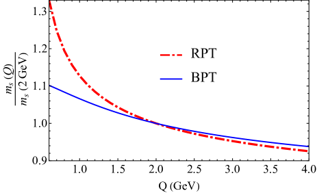
Figure 1:  Running mass of strange quark versus energy scale ($Q$) in presence of magnetic field $B=10^{18}\ G$ in RPT (full curve) and BPT (dashed curve) approaches.

Fig. 2 shows the comparison of the running coupling constant in the presence of $B=10^{18}$ G in both RPT and  BPT approaches. From this figure, we see that in all energy scales, the coupling constant in BPT is lower than that of RPT. Furthermore, the running coupling in BPT approach changes smoothly due to IR freezing effect.

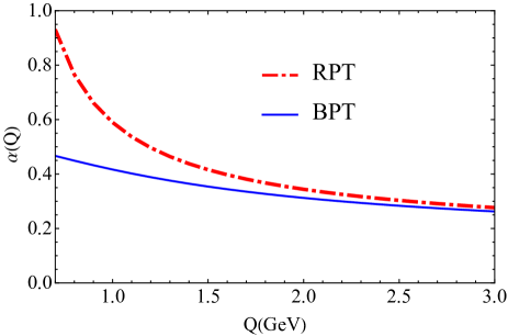
Figure 2: The comparison of QCD running coupling constant in presence of magnetic field $B=10^{18}\ G$ in RPT (dashed curve) and  BPT (dotted curve) approaches.

IV Thermodynamic potential up to the leading order

In grand canonical ensemble, the grand potential $\Omega$ at zero temperature is defined by

$$\dfrac{\Omega}{V}=\epsilon-{\mu}_{f}n_{f}-{\mu}_{e}n_{e},$$ (14)

where $V$ and $\epsilon$ are the volume and energy density of the system, respectively. $\mu_{f}$ and $n_{f}$ are quark’s chemical potential and density with flavor $f$. $\mu_{e}$ and $n_{e}$ are the electron chemical potential and electron number density, respectively. The quark number density, electron number density, longitudinal pressure and transverse pressure can be evaluated from the grand potential by

$$n_{i,e} = -\dfrac{1}{V}\dfrac{\partial\Omega}{\partial\mu_{i,e}},$$ (15)

$$P_{\lVert} = -\mathfrak{B}-\dfrac{\Omega}{V}+P_{CSC}-\dfrac{B^{2}}{8\pi},$$ (16)

$$P_{\bot} = -\mathfrak{B}-\dfrac{\Omega}{V}+P_{CSC}-M.B+\dfrac{B^{2}}{8\pi},$$ (17)

where $\mathfrak{B}$ is a free parameter interpreted as non-perturbative effects not included in perturbative expansion kurkela2010cold . To describe a more realistic quark matter, we have considered the color superconductivity pressure, $P_{CSC}$. This pressure is due to an appearing gap in the energy of the Cooper pairs in the Color-Flavor-Locked phase which is given as $P_{CSC}=\dfrac{\Delta^{2}(\mu_{u}+\mu_{d}+\mu_{s})^{2}}{3\pi^{2}}$, alford1999color where $\Delta$ is the gap parameter. The gap parameter depends on the magnetic field. Therefore, we consider different values for $\Delta$ ranging from $0$ to $100MeV$ in appendix B. This appendix shows that the maximum gravitational mass of SQS increases by increasing $\Delta$. In the following, we only obtain our results for $\Delta=100MeV$. In Eq. (17), $M$ is the magnetization of the system, which is calculated by $-\dfrac{\partial\Omega}{\partial B}$. To obtain the grand potential, we use the fact that $\Omega$ for each quark flavor can be divided into two perturbative and non-perturbative parts

$$\Omega=\Omega_{free}+\Omega_{2L},$$ (18)

where the non-perturbative part, $\Omega_{free}$, is the thermodynamic the potential of a free fermion moving in a uniform magnetic field which is given by

$$\frac{\Omega_{free}}{V}= -\,\sum_{f,j=0}^{\infty}\frac{|e_{f}B|}{2\pi^{2}}\bigg{\{}3(2-\delta_{j0})$$

$$\times\int_{0}^{(k_{z}^{f})_{F}}dk_{z}\frac{k_{z}{}^{2}}{\sqrt{m_{f}{}^{2}+k_{z}{}^{2}+2j|e_{f}B|}}\bigg{\}}$$

$$-\,\sum_{j=0}^{\infty}\frac{|eB|}{2\pi^{2}}\bigg{\{}(2-\delta_{j0})$$

$$\times\int_{0}^{(k_{z}^{e})_{F}}dk_{z}\frac{k_{z}{}^{2}}{\sqrt{m_{e}{}^{2}+k_{z}{}^{2}+2j|eB|}}\bigg{\}}$$ (19)

In above equation, $\left(k_{z}^{f}\right)_{F}$ denotes the quark fermi momentum with flavor $f$ which is $\sqrt{\mu_{f}^{2}-m_{f}^{2}-2j|e_{f}B|}$. $\left(k_{z}^{e}\right)_{F}$ denotes the electron fermi momentum with which is $\sqrt{\mu_{e}^{2}-m_{e}^{2}-2j|eB|}$. The perturbative part of the grand potential, $\Omega_{2L}$, is the QCD contribution at leading order for a system of quarks and gluons under strong magnetic field which is depicted by a two-loop diagram in Fig. 3.

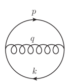
Figure 3: Two-loop diagram contributing to perturbative part of the grand potential at the leading order.

Appendix A shows the procedure to calculate the two-loop diagram at finite chemical potential. The masses of up and down quarks are negligible. For the mass of strange quark, we use the running mass from Eq. (11). The result of two-loop diagram (Eq. (A)), depends on the renormalization scale $Q$ that appears in mass and coupling constant through Eqs. (6) and (11). In the absence of strong magnetic field, phenomenological models propose $Q=2\pi\sqrt{T^{2}+\frac{\mu^{2}}{\pi^{2}}}$ for a massless quark with chemical potential $\mu$ at temperature $T$. At zero temperature, for a system composed of $N_{f}$ flavors, $Q=2\left({\sum_{f}\mu_{f}/3}\right)\equiv 2\overline{\mu}$ which can have a variation by a factor of 2 with respect to its central value schneider2003qcd ; bandyopadhyay2019pressure ; karmakar2019anisotropic .

Fig. 4 shows the ratio of $\dfrac{P_{\bot}-P_{\lVert}}{P_{\lVert}}$ versus baryon density, $n_{B}$, which indicates that the difference between longitudinal and transverse pressures decreases by increasing baryon number density. In section VIII, we show that the maximum gravitational masses due to these pressures ($P_{\lVert},P_{\bot}$) result in the same values approximately. Therefore our assumption for having an isotropic structure for the system under study is justified.

Fig. 5 shows the validity of our perturbative calculations. In this figure, the ratio of calculated pressure up to the leading order in $\alpha_{s}$ to the pressure of free quarks is presented. As the figure shows, this ratio tends to unity by increasing the renormalization scale $Q$ for three choices of renormalization scale in RPT approach. Such an asymptotic behavior is necessary for any perturbative method, which shows that the perturbative part is lower than the non-perturbative part. Also, the non-perturbative contribution decreases by increasing the energy due to the asymptotic freedom of the coupling constant. Furthermore, we have imposed the following constraints in our perturbative calculations:

i) To establish the causality, the ratio of the speed of sound to the speed of light in the vacuum should be lower than unity.

ii) To establish dynamical stability, the adiabatic index should be lower than $\dfrac{4}{3}$ panah2019contraction .

iii) The relation between pressure and energy density is in such a way that $\epsilon+P\geq 0$ and $\epsilon\geq\mid P\mid$ roupas2021qcd .

iv) To describe a realistic SQS, the minimum value of the baryon number density should be higher than the nuclear saturation density $(n_{B}=0.16fm^{-3})$.

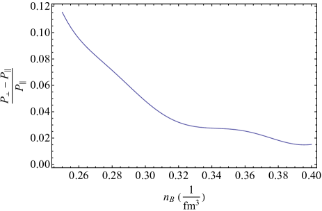
Figure 4: The ratio of $\dfrac{P_{\bot}-P_{\lVert}}{P_{\lVert}}$ versus baryon number density.

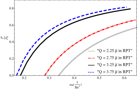
Figure 5: The ratio of calculated pressure up to leading order in $\alpha_{s}$ to the pressure of the free quarks versus renormalization scale $Q$ for three choices of renormalization scale in RPT approach.

V Equation of state and stability conditions

In this section, we use the numerical results from the grand potential presented in the previous section to derive the EoS of a stable SQS. We derive the relationship between the total energy density and pressure (EoS) to evaluate the star’s maximum mass and corresponding radius. Therefore, we can derive the EoS using Eqs. (15-IV) and (A) from the following relation

$$\varepsilon=-P_{\lVert}+\mu_{u}n_{u}+\mu_{d}n_{d}+\mu_{s}n_{s}.$$ (20)

It should be noted that in deriving the EoS, we have considered beta equilibrium and charge neutrality conditions blaschke2001physics . For beta equilibrium, we have the following weak processes.

$$d\longrightarrow u+e+\bar{\nu}_{e},~{}~{}~{}\&~{}~{}~{}u+e\longrightarrow d+\nu_{e},$$

$$s\longrightarrow u+e+\bar{\nu}_{e},~{}~{}~{}\&~{}~{}~{}u+e\longrightarrow s+\nu_{e},$$

$$s+u\longleftrightarrow d+u,$$ (21)

which lead to the following conditions

$$\mu_{s}=\mu_{d}\equiv\mu,~{}~{}~{}\&~{}~{}~{}\mu_{u}=\mu-\mu_{e}.$$ (22)

The mean free path of neutrinos is considerably larger than the size of the star, and therefore their chemical potential can be neglected in the calculations. For charge neutrality, the following condition must be imposed.

$$\frac{2}{3}n_{u}-\frac{1}{3}n_{d}-\frac{1}{3}n_{s}-n_{e}=0,$$ (23)

where $n_{e}$, the electron number density, is equal to

$$n_{e}=\dfrac{eB}{(2\pi)^{2}}\mu_{e}^{2}.$$ (24)

Furthermore, for the existence of SQS, another condition must be implemented, which implies that the minimum energy per baryon should be lower than that of the most stable nuclei $\left({}^{56}Fe\right)$ weber2005strange

$$\dfrac{\epsilon}{n_{B}}\leq 0.93GeV,$$ (25)

where $n_{B}$, the baryon number density, is obtained by quark number densities as

$$n_{B}=\dfrac{n_{u}+n_{d}+n_{s}}{3}.$$ (26)

VI Thermodynamic properties of strange quark matter in strong magnetic field

In this section, we investigate our results for thermodynamic properties such as baryon density, speed of sound, adiabatic index, and also the EoS of SQM in RPT and BPT, respectively.

VI.1 Results in RPT

Using Eqs. (15), (IV) and (A), the quark number densities as functions of quark chemical potentials are obtained. Then, we use Eqs. (22), (23), (24) and (26) to get the allowed values of chemical potentials for the quarks. The values of $\mathfrak{B}$ in Eq. (16) are chosen in such a way to get zero total pressure at the surface of the star where the baryon density is minimum. If we neglect interaction between quarks, $\mathfrak{B}$ has the role of MIT bag constant ranging from $41.58\ MeV/fm^{3}$ to $319.31\ MeV/fm^{3}$ aziz2019constraining . The EoS of SQM for different choices of renormalization scale is shown in Fig. 6. The minimum value for the renormalization scale starts at a point from which the perturbative calculation is valid. Furthermore, for renormalization scales more than $Q=3.25\overline{\mu}$, the results do not change significantly. From this figure, it is understood that the EoS becomes stiffer by increasing the renormalization scale. To establish causality condition, the ratio of the speed of sound to the speed of light in vacuum $\left(\sqrt{dP/d\epsilon}\right)$ must be lower than unity. Fig. 7 shows that our results satisfy the causality condition for different choices of renormalization scale.

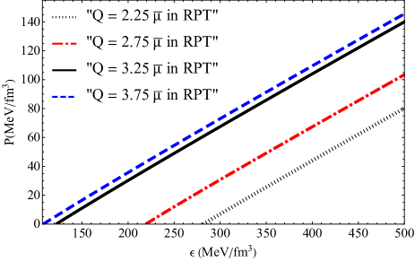
Figure 6: Pressure versus energy density (EoS) for different choices of renormalization scale in RPT.

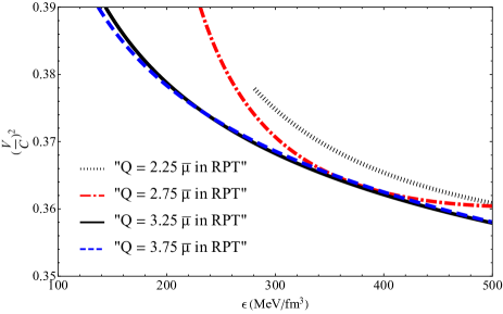
Figure 7:  Squared speed of sound versus energy density for different choices of renormalization scale in RPT.

It is known that for dynamical stability the adiabatic index $\Gamma=dP/d\epsilon\dfrac{(P+\epsilon)}{P}$ must be higher than $4/3$ bardeen1966catalogue ; knutsen1988stability ; mak2013isotropic ; panah2019white ; panah2019contraction . The adiabatic index has been presented as a function of energy density in Fig. 8. As one can see from this figure, the condition $\Gamma>4/3$ is satisfied for all renormalization scales.

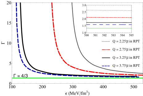
Figure 8: Adiabatic index versus the ratio of baryon density to nuclear saturation density for different choices of renormalization scale in RPT.

VI.2 Results in BPT

Now we perform the calculations for BPT the same as we did for RPT. Here, $M_{B}$ in Eq. (6) is equal to $\sqrt{2\pi\sigma}$. The parameter $\sigma$ is the string tension which is equal to $0.18\ GeV^{2}$ deur2016qcd . Assuming the same constraints presented in section V, we obtain the EoS of the SQM for different renormalization scales. For the values $Q>2.75\overline{\mu}$, the results for the structural properties of the star do not change significantly.

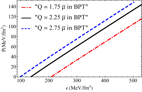
Figure 9: Pressure versus energy density (EoS) for different choices of renormalization scale in BPT.

The diagrams of the speed of sound and adiabatic index in BPT are shown in Figs. 10 and 11. These diagrams indicate that the constraints related to the speed of sound and adiabatic indices are satisfied well by our obtained EoSs.

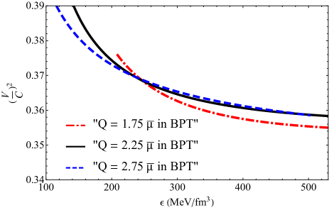
Figure 10: Squared speed of sound versus energy density for different choices of renormalization scale in BPT.

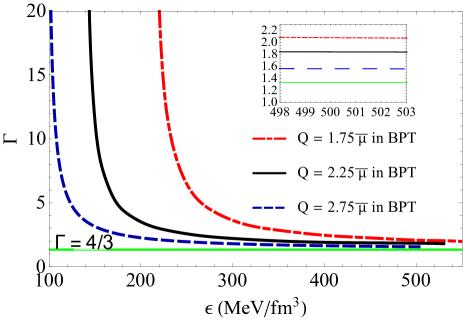
Figure 11:  Adiabatic index versus the ratio of baryon density to nuclear saturation density for different choices of renormalization scale in BPT.

VII Magnetized strange quark star structure

After computing the EoS, the structure of a hydrostatic and non-rotating strange stars can be obtained by general relativistic equations of hydrostatics. Here, the relation between mass and radius of the star is found by solving TOV equations oppenheimer1939massive ,

$$\ dM(r) = 4\pi r^{2}\epsilon(r)dr,$$ (27)

$$\frac{dP(r)}{dr} = \dfrac{G\left[P(r)+\epsilon(r)\right]\left[M(r)+4\pi r^{3}P(r)\right]}{r\left(2GM(r)-r\right)},$$ (28)

where $G$ and $r$ are the Newton gravitational constant and radial coordinate of the star, respectively. For different central pressure values, different gravitational masses and radii are obtained. In the following, the results for different values of the renormalization scale in RPT and BPT approaches are discussed.

Our results for the structural properties of SQS in RPT have been presented in Figs. 12 and 13. The limiting behavior of mass in Fig. 12 shows the maximum gravitational mass of SQS. From this figure, we see that the maximum gravitational mass increases by increasing the renormalization scale, $Q$, which corresponds to stiffer EoSs (Fig. 9). This behavior indicates that stiffer EoS leads to higher gravitational mass for SQS in our model. Our results for maximum gravitational mass and corresponding radius in RPT are given in Table 1. Previously

Figure 12:  Mass versus energy density for different choices of renormalization scale in RPT.

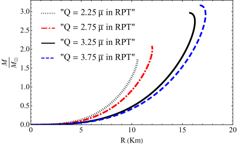
Figure 13:  Mass-radius diagram for different choices of renormalization scale in RPT.

the maximum gravitational mass of the SQS by perturbative calculation in the absence of magnetic field was obtained in Refs. fraga2005role ; kurkela2010cold . In Ref. kurkela2010cold , by using regular perturbation theory up to second order of coupling constant, the maximum mass of a pure strange quark star was obtained to be $2.75M_{\odot}$. From Table. 1, we see that in RPT model, the maximum mass of SQS can reach the value $M\simeq 3.17M_{\odot}$ which is considerably higher than that of in the absence of magnetic field calculated in Refs. kurkela2010cold ; fraga2005role .

Table 1: maximum gravitational mass and the corresponding radius of SQS for different renormalization scales in RPT.

$Q$/$\overline{\mu}$	$\dfrac{M}{M_{\odot}}$	$R(km)$	$R_{Sch}(km)$	$z$	$\dfrac{M_{BB}}{{M}_{\odot}}$	$\sigma(10^{-1})$
2.25	1.72	10.56	5.07	0.38	3.18	4.80
2.75	2.09	11.98	6.16	0.43	3.61	5.14
3.25	2.97	15.67	8.76	0.50	4.72	5.59
3.75	3.17	16.53	9.34	0.52	4.98	5.65

Now we discuss the maximum gravitational mass and the corresponding radius of the SQS in BPT. Figs. 14 and 15 show that by increasing $Q$, the maximum mass increases. Our

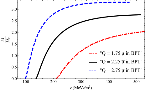
Figure 14:  Mass versus energy density for different choices of renormalization scale in BPT.

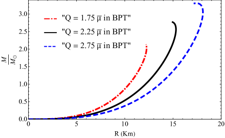
Figure 15: Mass-radius diagram for different choices of renormalization scale in BPT.

results for the maximum gravitational mass and the corresponding radius in BPT are given in Table 2. By comparing our results in two approaches from Tables 1 and 2, we can conclude that the gravitational mass of strange quark star in BPT is higher than that of RPT. It seems that it is originated from the behavior of the coupling constant. The coupling constant in BPT is smaller and runs slower than that in RPT.

Table 2: The values of the mass and the corresponding radius of the star in different renormalization scales in BPT

$Q$/$\overline{\mu}$	$\dfrac{M}{M_{\odot}}$	$R(Km)$	$R_{Sch}(km)$	$z$	$\dfrac{M_{BB}}{{M}_{\odot}}$	$\sigma(10^{-1})$
1.75	2.11	12.22	6.22	0.43	3.68	5.09
2.25	2.77	14.96	8.17	0.48	4.51	5.46
2.75	3.31	17.26	9.76	0.52	5.20	5.65

VII.1 Compactness

Compactness is a quantity that gives us information about the strength of gravity of compact objects. The compactness of a spherical object is usually defined in the following form

$$\sigma=\frac{R_{Sch}}{R},$$ (29)

where $R_{Sch}$ and $R$ are the Schwarzschild radius and radius of compact object, respectively. Our results for the compactness are presented in Tables. 1 and 2, which indicate that by increasing renormalization scale ($Q$), the compactness from the perspective of a distant observer (or an observer outside the compact object) increases.

VII.2 Gravitational Redshift

Another quantity that gives us information on the strength of gravity is related to the gravitational redshift. The gravitational redshift is given by

$$z=\frac{1}{\sqrt{1-\frac{2GM}{c^{2}R}}}-1,$$ (30)

where $M$ and $R$ are related to the compact star’s mass and radius, respectively. The results related to the gravitational redshift are given in Tables. 1 and 2. These results indicate that the gravitational redshift increases by increasing the renormalization scale. But this quantity is less than $1$ for magnetized SQSs.

VII.3 Buchdahl-Bondi Bound

Here, we want to study the upper mass limit of a static spherical quark star with uniform density in GR, the so-called Buchdahl theorem buchdahl1959general . The GR compactness limit is given by buchdahl1959general

$$M\leq M_{BB}=\frac{4c^{2}R}{9G},$$ (31)

in which the upper mass limit is $M_{\max}=\frac{4c^{2}R}{9G}$. Our numerical results in Tables. 1 and 2, confirm that the obtained masses of magnetized SQSs in GR respects the equation (31).

Our calculations from the redshift ($z$) and Buchdahl-Bondi bound ($M_{BB}$) of magnetized SQSs confirm that these compact objects cannot be black holes, because the values of redshift for these compact objects are finite ($z<1$), and also the maximum mass of these compact objects are less than Buchdahl-Bondi bound ($M_{\max}<M_{BB}$).

VIII The effect of the anisotropy on the structure of the magnetized SQS

In this section, we consider the magnetic fields with the values $10^{18}\ G$, $2\times 10^{18}\ G$ and $3\times 10^{18}\ G$ and calculate the maximum mass of the SQS by considering longitudinal pressure, $P_{\lVert}$ and the transverse pressure, $P_{\bot}$, in TOV equations separately. The maximum gravitational mass and the corresponding radius evaluated by $P_{\lVert}$, are denoted by $M_{\lVert}$ and $R_{\lVert}$ and the ones obtained by $P_{\bot}$, are denoted by $M_{\bot}$ and $R_{\bot}$, respectively. Fig. 16 and Table. 3 show our results in RPT by assuming the renormalization scale $Q=3.75\overline{\mu}$. As we can see from the results, there is no distinguishable difference between $M_{\lVert}$ and $M_{\bot}$ for the magnetic field $10^{18}\ G$ and $2\times 10^{18}\ G$. But for $B=3\times 10^{18}\ G$ this difference is obvious and the isotropic structure is not a good approximation. We have defined the $\delta$ parameter as the measure of the anisotropy of the star which is equal to $\dfrac{M_{\lVert}-M_{\bot}}{\left(M_{\lVert}+M_{\bot}\right)/2}$ chu2018quark . The values of the $\delta$ parameter for different magnetic fields have been presented in Table. 3. As we can see from this table, this parameter is negligible for the magnetic fields less than about $2\times 10^{18}\ G$. The threshold magnetic field from which an anisotropic approach begins to be significant lies in the interval $2\times 10^{18}G<B<3\times 10^{18}G$. Such behavior can also be seen in Ref. chu2018quark within the extended confined isospin-density-dependent mass model. Therefore, it seems that considering the isotropic structure for a SQS under the magnetic fields $B<2\times 10^{18}G$ is reasonable in our models.

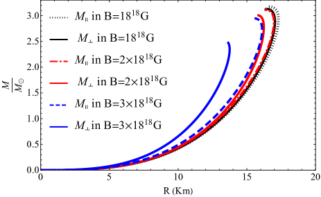
Figure 16:  Mass-radius diagram for different magnetic fields in RPT and $Q=3.75\overline{\mu}$. $M_{\lVert}$ and $M_{\bot}$ are the maximum mass calculated by the pressures $P_{\lVert}$ and $P_{\bot}$, respectively.

Table 3: The values of the maximum mass and the corresponding radius of the SQS for different magnetic fields in RPT and $Q=3.75\overline{\mu}$. $M_{\lVert}$ and $M_{\bot}$ are the maximum mass calculated by the pressures $P_{\lVert}$ and $P_{\bot}$, respectively. $R_{\lVert}$ and $R_{\bot}$ are their corresponding radii.

$B(G)$	$\dfrac{M_{\lVert}}{M_{\odot}}$	$R_{\lVert}(Km)$	$\dfrac{M_{\bot}}{M_{\odot}}$	$R_{\bot}(Km)$	$\delta(\%)$
$10^{18}$	3.17	16.53	3.13	16.35	1.27
$2\times 10^{18}$	3.11	16.16	3.01	15.67	3.27
$3\times 10^{18}$	2.95	15.57	2.49	13.40	17

IX Conclusions and Outlook

In this paper, we first introduced QCD Feynman rules in the presence of a strong magnetic field. Then we performed perturbative calculations of the thermodynamic potential of a strange quark matter (SQM) up to O($\alpha_{s}$) in the presence of magnetic field $B=10^{18}\ G$. We used two approaches in our perturbative calculations: i) QCD without IR freezing effect in regular perturbation theory (RPT) and ii) QCD with IR freezing effect in background perturbation theory (BPT). The thermodynamic potential of SQM was computed by separating it into non-perturbative and perturbative parts. The non-perturbative part contained the interaction of quarks with the magnetic field, and the perturbative part included QCD interaction between quarks. The perturbative part contained a two-loop diagram added to the thermodynamic potential of a moving fermion in a uniform magnetic field as the non-perturbative part. Using the obtained thermodynamic potential and also considering the stability conditions of SQM, thermodynamic properties such as quark number densities, speed of sound, adiabatic index, and also the EoSs of strange quark stars (SQSs) were obtained in RPT and BPT models. Then by employing the obtained EoSs, we calculated the structure properties of SQSs. Moreover, the redshift, compactness, and Buchdahl-Bondi bound of the SQSs were calculated to show that these compact objects cannot be black holes. Then, the anisotropic effect on the structure of SQS in our models under different magnetic fields was calculated. it was shown that the threshold magnetic field from which an anisotropic approach begins to be significant lies in the interval $2\times 10^{18}G<B<3\times 10^{18}G$. The maximum mass of the SQS under the magnetic field $B=10^{18}\ G$ was obtained $3.17M_{\odot}$ and $3.31M_{\odot}$ in RPT and BPT, respectively, which is considerably higher than those of Bag models and NJL theories. Furthermore, it is notable that some of our results for the maximum gravitational mass are outside the limits obtained by observational constraints for neutron stars. Therefore an observed violation of those limits might be a piece of evidence for SQS. For example the compact object with the mass $2.5-2.67M_{\odot}$ in GW190814 miao2021bayesian or the remnant mass of GW190425 sedaghat2021compact might be SQSs.

X Appendix

Appendix A Calculation of the thermodynamic potential of the two-loop diagram

By using the Feynman rules introduced in section III we have

$$\dfrac{\Omega_{2L}}{V}= \dfrac{g^{2}d_{A}}{2}$$

$$\times\sum_{n,j=0}^{\infty}\int\dfrac{d^{4}p}{(2\pi)^{4}}\int\dfrac{d^{4}k}{(2\pi)^{4}}\dfrac{(-1)^{j+n}e^{-(p_{\perp}^{2}+k_{\perp}^{2})/{\lvert e_{f}B\rvert}}}{(p-k)^{2}}$$

$$\times\dfrac{Tr\left[\gamma^{\mu}D_{j}(\lvert e_{f}B\rvert,p)\gamma_{\mu}D_{n}(\lvert e_{f}B\rvert,k)\right]}{\mathcal{A}_{1}\mathcal{A}_{2}},$$ (32)

where $\mathcal{A}_{1}=(p_{0}+i\mu)^{2}+(p_{3}^{2}+m_{f}^{2}+2j\lvert e_{f}B\rvert)$ and $\mathcal{A}_{2}=(k_{0}+i\mu)^{2}+(k_{3}^{2}+m_{f}^{2}+2n\lvert e_{f}B\rvert)$. Also, $d_{A}$ is $N_{c}^{2}-1$. The summation is over Landau levels, and $D_{j}(\lvert e_{f}B\rvert,p)$ and $D_{n}(\lvert e_{f}B\rvert,k)$ are functions in terms of generalized Laguerre polynomials and Dirac Gamma matrices in Euclidean space. To obtain the contribution (A), we use a very useful method derived in Ref. ghicsoiu2017high which is referred to as cutting rules. Based on this method, the evaluation of the Feynman integrals at zero temperature and finite chemical potential is reduced to the evaluation of three-dimensional phase space integrals over on-shell amplitudes at $T=\mu=0$. Indeed, the one point irreducible N-loop n-point Feynman diagram, $F(P_{k},\mu)$, can be simplified as:

$$F(P_{k},\mu)=$$ (33)

$$F_{0-cut}(P_{k})+F_{1-cut}(P_{k},\mu)+...+F_{N-cut}(P_{k},\mu),$$

where $F_{0-cut}(P_{k})$ is the original diagram computed at zero chemical potential, and the other terms are contributions resulting from the cutting procedure. Indeed, $F_{j-cut}(P_{k},\mu)$ represents the sum of all diagrams in which the j number of internal fermion propagators have been cut from the original graph. In the following, we explain the steps in the cutting procedure:

1. The cut propagators are removed from the original

graph

2. The remaining $N-j$- loop $n+2j$- point amplitude

is computed by considering the point that the all

external momenta are real-valued.

3. The cut momenta $p_{i}$ is set on-shell by inserting

$({p_{0}})_{i}=iE_{i}$.

4. The remaining expression is integrated over the cut

three-dimensional momenta $p_{i}$ with the weight

$\dfrac{-\theta(\mu-E_{i})}{2E_{i}}$, where for a quark moving in a uniform

magnetic field $B$ at the $j$th Landau level, $E_{p}$ is equal

to $\sqrt{p_{3}^{2}+m_{f}^{2}+2j\lvert e_{f}B\rvert}$.

Notably, $F_{0-cut}(P_{k})$ has no dependence on chemical potential, and according to Eq. (15), it has no contribution in quark number densities. Therefore, it is has been removed from calculations. By following the cutting procedure and Eq. (A), we get

$$\dfrac{\Omega_{2L}}{V}=F_{1-cut}+F_{2-cut},$$ (34)

where $F_{1-cut}$ and $F_{2-cut}$ are given as

$$F_{1-cut} =-2\times\dfrac{g^{2}d_{A}}{2}\bigg{\{}\sum_{n,j=0}^{\infty}\int\dfrac{\theta(\mu-E_{p})}{2E_{p}}\dfrac{d^{3}\mathbf{p}}{(2\pi)^{3}}$$

$$\times\int\dfrac{d^{4}k}{(2\pi)^{4}}I_{1}\bigg{\}}_{p_{0}=iE_{p}},$$ (35)

$$F_{2-cut} =\dfrac{g^{2}d_{A}}{2}\bigg{\{}\sum_{n,j=0}^{\infty}\int\dfrac{\theta(\mu-E_{p})}{2E_{p}}\dfrac{d^{3}\mathbf{p}}{(2\pi)^{3}}$$

$$\times\int\dfrac{\theta(\mu-E_{k})}{2E_{k}}\dfrac{d^{3}\mathbf{k}}{(2\pi)^{3}}I_{2}\bigg{\}}_{p_{0}=iE_{p},k_{0}=iE_{k}},$$ (36)

where, $I_{1}$ and $I_{2}$ are defined as

$$I_{1} =(-1)^{j+n}e^{-(p_{\perp}^{2}+k_{\perp}^{2})/{\lvert e_{f}B\rvert}}$$

$$\times\dfrac{Tr\left[\gamma^{\mu}D_{j}(\lvert e_{f}B\rvert,p)\gamma_{\mu}D_{n}(\lvert e_{f}B\rvert,k)\right]}{({k_{0}}^{2}+{E_{k}}^{2})((p_{0}-k_{0})^{2}+(\mathbf{p}-\mathbf{k})^{2})},$$ (37)

$$I_{2} =(-1)^{j+n}e^{-(p_{\perp}^{2}+k_{\perp}^{2})/{\lvert e_{f}B\rvert}}$$

$$\times\dfrac{Tr\left[\gamma^{\mu}D_{j}(\lvert e_{f}B\rvert,p)\gamma_{\mu}D_{n}(\lvert e_{f}B\rvert,k)\right]}{(p_{0}-k_{0})^{2}+(\mathbf{p}-\mathbf{k})^{2}}.$$ (38)

Due to the Landau quantization of transverse momentums at the $j$th Landau level, we set $\sqrt{2j\lvert e_{f}B\rvert}$ and $\sqrt{2(j+1)\lvert e_{f}B\rvert}$ for the lower and upper limits of the transverse momentum integrals, respectively. To calculate Eq. (34), we need to sum over all the terms corresponding to $n$th and $j$th Landau levels. Indeed for each pair $(n,j)$ which appear as Landau levels in propagators of quarks, there is an integral which should be computed. It should be noted that by multiplying a factor $-1/2$ in Eq. (34), originated from perturbative expansion kapusta2006finite , we obtain Eq. (A).

$$\dfrac{\Omega_{2L}}{V}=\dfrac{g^{2}d_{A}}{2}\sum_{n,j=0}^{\infty}\bigg{\{}\int\dfrac{d^{4}p}{(2\pi)^{4}}\int\dfrac{d^{4}k}{(2\pi)^{4}}I_{1}(-\theta(\mu-E_{q}))$$

$$-\dfrac{1}{2}\int\dfrac{d^{4}p}{(2\pi)^{4}}\int\dfrac{d^{4}k}{(2\pi)^{4}}I_{2}(-\theta(\mu-E_{q}))(-\theta(\mu-E_{p}))\bigg{\}},$$ (39)

Appendix B Investigating the effect of the gap parameter in maximum gravitational mass of SQS

By using different values of $\Delta$ in Eq. (16), we have plotted mass-radius diagrams for SQS under the magnetic field $B=10^{18}G$. As the Table 4 and Figures 17 and 18 show, the maximum gravitational mass of SQS increases by increasing $\Delta$ for both RPT and BPT models. Furthermore, it is notable that our calculations show that the impact of $\Delta$ on the structure of SQS begins to be significant from $\Delta>25MeV$.

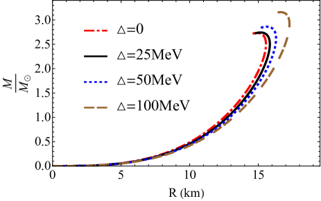
Figure 17:  Mass-radius diagram for different values of $\Delta$ parameter in RPT ($Q=3.75\overline{\mu}$) model.

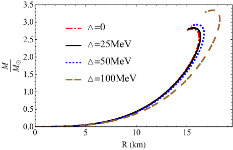
Figure 18:  Mass-radius diagram for different values of $\Delta$ parameter in BPT ($Q=2.75\overline{\mu}$) model.

Table 4: The values of the maximum mass and the corresponding radius of SQS for different values of $\Delta$ in RPT($Q=3.75\overline{\mu}$) and BPT($Q=2.75\overline{\mu}$) models.

	RPT	RPT	BPT	BPT
$\Delta(MeV)$	$\dfrac{M_{\lVert}}{M_{\odot}}$	$R_{\lVert}(Km)$	$\dfrac{M_{\lVert}}{M_{\odot}}$	$R_{\lVert}(Km)$
$0$	2.71	14.81	2.84	15.80
$25$	2.75	15.00	2.87	15.89
$50$	2.86	15.65	2.95	16.04
$100$	3.17	16.53	3.31	17.26

References

- (1) S.L. Shapiro, S.A. Teukolsky, Black holes, white dwarfs, and neutron stars: The physics of compact objects (John Wiley & Sons, 2008)
- (2) A. Schmitt, Dense matter in compact stars: A pedagogical introduction, vol. 811 (Springer, 2010)
- (3) N.K. Glendenning, Compact stars: Nuclear physics, particle physics and general relativity (Springer Science & Business Media, 2012)
- (4) H. Karttunen, P. Kröger, H. Oja, M. Poutanen, K.J. Donner, Fundamental astronomy (Springer, 2016)
- (5) M. Camenzind, Compact objects in astrophysics (Springer, 2007)
- (6) L. Rezzolla, P. Pizzochero, D.I. Jones, N. Rea, I. Vidaña, The physics and astrophysics of neutron Stars (Springer, 2018)
- (7) M. Gell-Mann, in Murray Gell-Mann: Selected Papers (World Scientific, 2010), pp. 151–152
- (8) G. Zweig, An su model for strong interaction symmetry and its breaking. Tech. rep., CM-P00042884 (1964)
- (9) J.I. Friedman, H.W. Kendall, Annual Review of Nuclear Science 22(1), 203 (1972)
- (10) D. Ivanenko, D. Kurdgelaidze, Hypothesis concerning quark stars. Tech. rep., Moscow State Univ. (1965)
- (11) N. Itoh, Progress of Theoretical Physics 44(1), 291 (1970)
- (12) P. Haensel, J. Zdunik, R. Schaefer, Astronomy and Astrophysics 160, 121 (1986)
- (13) A. Bodmer, Physical Review D 4(6), 1601 (1971)
- (14) E. Witten, Physical Review D 30(2), 272 (1984)
- (15) E. Farhi, R.L. Jaffe, Physical Review D 30(11), 2379 (1984)
- (16) E. Farhi, Comments on Nuclear and Particle Physics 16(MIT-CTP-1343), 289 (1986)
- (17) C. Alcock, E. Farhi, A. Olinto, The Astrophysical Journal 310, 261 (1986)
- (18) S. Chakrabarty, Physical Review D 43(2), 627 (1991)
- (19) J. Madsen, in Hadrons in dense matter and hadrosynthesis (Springer, 1999), pp. 162–203
- (20) F. Weber, Progress in Particle and Nuclear Physics 54(1), 193 (2005)
- (21) B. Holdom, J. Ren, C. Zhang, Physical Review Letters 120(22), 222001 (2018)
- (22) K. Schertler, C. Greiner, P. Sahu, M. Thoma, Nuclear Physics A 637(3), 451 (1998)
- (23) D. Blaschke, H. Grigorian, D. Voskresensky, Astronomy & Astrophysics 368(2), 561 (2001)
- (24) G. Burgio, H.J. Schulze, F. Weber, Astronomy & Astrophysics 408(2), 675 (2003)
- (25) M. Alford, M. Braby, M. Paris, S. Reddy, The Astrophysical Journal 629(2), 969 (2005)
- (26) F.C. Michel, Physical Review Letters 60(8), 677 (1988)
- (27) A. Drago, A. Lavagno, Physics Letters B 511(2-4), 229 (2001)
- (28) I. Bombaci, in The Eleventh Marcel Grossmann Meeting: On Recent Developments in Theoretical and Experimental General Relativity, Gravitation and Relativistic Field Theories (In 3 Volumes) (World Scientific, 2008), pp. 605–628
- (29) W. Greiner, H. Stöcker, The Nuclear Equation of State: Part A: Discovery of Nuclear Shock Waves and the EOS, vol. 216 (Springer Science & Business Media, 2013)
- (30) B. Eslam Panah, T. Yazdizadeh, G.H. Bordbar, The European Physical Journal C 79(10), 815 (2019)
- (31) J. Sedaghat, S. Zebarjad, G. Bordbar, B. Eslam Panah, arXiv preprint arXiv:2104.00544 (2021)
- (32) C. Kouveliotou, S. Dieters, T. Strohmayer, J. Van Paradijs, G. Fishman, C. Meegan, K. Hurley, J. Kommers, I. Smith, D. Frail, et al., Nature 393(6682), 235 (1998)
- (33) R. Turolla, S. Zane, A. Watts, Reports on Progress in Physics 78(11), 116901 (2015)
- (34) D. Lai, S.L. Shapiro, The Astrophysical Journal 383, 745 (1991)
- (35) G. Chanmugam, Annual Review of Astronomy and Astrophysics 30(1), 143 (1992)
- (36) D. Lai, Reviews of Modern Physics 73(3), 629 (2001)
- (37) E.J. Ferrer, V. de La Incera, J.P. Keith, I. Portillo, P.L. Springsteen, Physical Review C 82(6), 065802 (2010)
- (38) H. Sotani, T. Tatsumi, Monthly Notices of the Royal Astronomical Society 447(4), 3155 (2015)
- (39) R.C. Duncan, C. Thompson, The Astrophysical Journal 392, L9 (1992)
- (40) L. Landau, JETP (Sov. Phys.) 3, 920 (1956)
- (41) L. Landau, E. Lifshitz, Quantum Mechanics (Pergamon Press, 1977)
- (42) F. Kayanikhoo, K. Naficy, G.H. Bordbar, The European Physical Journal A 56(1), 2 (2020)
- (43) S. Chakrabarty, Physical Review D 54(2), 1306 (1996)
- (44) D.A. Fogaça, S. Sanches Jr, T. Motta, F.S. Navarra, Physical Review C 94(5), 055805 (2016)
- (45) V. Dexheimer, B. Franzon, R. Gomes, R. Farias, S. Avancini, S. Schramm, Physics Letters B 773, 487 (2017)
- (46) H. Sotani, T. Tatsumi, Monthly Notices of the Royal Astronomical Society 467(1), 1249 (2017)
- (47) S. Chakrabarty, P. Sahu, Physical Review D 53(8), 4687 (1996)
- (48) P.C. Chu, X.H. Li, H.Y. Ma, B. Wang, Y.M. Dong, X.M. Zhang, Physics Letters B 778, 447 (2018)
- (49) M.A. Andreichikov, V. Orlovsky, Y.A. Simonov, Physical Review Letters 110(16), 162002 (2013)
- (50) E.S. Fraga, P. Romatschke, Physical Review D 71(10), 105014 (2005)
- (51) A. Kurkela, P. Romatschke, A. Vuorinen, Physical Review D 81(10), 105021 (2010)
- (52) K. Bhattacharya, arXiv preprint arXiv:0705.4275 (2007)
- (53) I.A. Shovkovy, in Strongly Interacting Matter in Magnetic Fields (Springer, 2013), pp. 13–49
- (54) T. Kojo, N. Su, Physics Letters B 726(4-5), 839 (2013)
- (55) V.A. Miransky, I.A. Shovkovy, Physics Reports 576, 1 (2015)
- (56) M. Vysotsky, JETP letters 92(1), 15 (2010)
- (57) Y.A. Simonov, Physics of Atomic Nuclei 74(8), 1223 (2011)
- (58) A. Deur, S.J. Brodsky, G.F. de Téramond, Progress in Particle and Nuclear Physics 90, 1 (2016)
- (59) A. Deur, V. Burkert, J.P. Chen, W. Korsch, Physics Letters B 665(5), 349 (2008)
- (60) K. Ackerstaff et al, The European Physical Journal C 7(4), 571 (1999)
- (61) S.J. Brodsky, R. Shrock, Physics Letters B 666(1), 95 (2008)
- (62) E. Ferrer, V. De la Incera, X. Wen, Physical Review D 91(5), 054006 (2015)
- (63) A. Badalian, B. Bakker, Physical Review D 100(5), 054036 (2019)
- (64) J. Vermaseren, S. Larin, T. Van Ritbergen, Physics Letters B 405(3-4), 327 (1997)
- (65) M. Tanabashi, K. Hagiwara, K. Hikasa, K. Nakamura, Y. Sumino, F. Takahashi, J. Tanaka, K. Agashe, G. Aielli, C. Amsler, et al., (2018)
- (66) M. Alford, K. Rajagopal, F. Wilczek, Nuclear Physics B 537(1-3), 443 (1999)
- (67) R. Schneider, arXiv preprint hep-ph/0303104 (2003)
- (68) A. Bandyopadhyay, B. Karmakar, N. Haque, M.G. Mustafa, Physical Review D 100(3), 034031 (2019)
- (69) B. Karmakar, R. Ghosh, A. Bandyopadhyay, N. Haque, M.G. Mustafa, Physical Review D 99(9), 094002 (2019)
- (70) Z. Roupas, G. Panotopoulos, I. Lopes, Physical Review D 103(8), 083015 (2021)
- (71) D. Blaschke, N.K. Glendenning, A. Sedrakian, Physics of neutron star interiors, vol. 578 (Springer Science & Business Media, 2001)
- (72) A. Aziz, S. Ray, F. Rahaman, M. Khlopov, B. Guha, International Journal of Modern Physics D 28(13), 1941006 (2019)
- (73) J.M. Bardeen, K.S. Thorne, D.W. Meltzer, The Astrophysical Journal 145, 505 (1966)
- (74) H. Knutsen, Monthly Notices of the Royal Astronomical Society 232(1), 163 (1988)
- (75) M. Mak, T. Harko, The European Physical Journal C 73(10), 1 (2013)
- (76) B. Eslam Panah, H. Liu, Physical Review D 99(10), 104074 (2019)
- (77) J.R. Oppenheimer, G.M. Volkoff, Physical Review 55(4), 374 (1939)
- (78) H.A. Buchdahl, Physical Review 116(4), 1027 (1959)
- (79) Z. Miao, J.L. Jiang, A. Li, L.W. Chen, The Astrophysical Journal Letters 917(2), L22 (2021)
- (80) I. Ghişoiu, T. Gorda, A. Kurkela, P. Romatschke, M. Säppi, A. Vuorinen, Nuclear Physics B 915, 102 (2017)
- (81) J.I. Kapusta, C. Gale, Finite-temperature field theory: Principles and applications (Cambridge University Press, 2006)