Cluster Structures with Machine Learning Support in Neutron Star M-R relations

Abstract

Neutron stars (NS) are compact objects with strong gravitational fields, and a matter composition subject to extreme physical conditions. The properties of strongly interacting matter at ultra-high densities and temperatures impose a big challenge to our understanding and modelling tools. Some difficulties are critical, since one cannot reproduce such conditions in our laboratories or assess them purely from astronomical observations. The information we have about neutron star interiors are often extracted indirectly, e.g., from the star mass-radius relation. The mass and radius are global quantities and still have a significant uncertainty, which leads to great variability in studying the micro-physics of the neutron star interior. This leaves open many questions in nuclear astrophysics and the suitable equation of state (EoS) of NS. Recently, new observations appear to constrain the mass-radius and consequently has helped to close some open questions. In this work, utilizing modern machine learning techniques, we analyze the NS mass-radius (M-R) relationship for a set of EoS containing a variety of physical models. Our objective is to determine patterns through the M-R data analysis and develop tools to understand the EoS of neutron stars in forthcoming works.

1 Introduction

Neutron stars (NS) are one of the densest objects in the Universe, and the geometry of the spacetime around it deviates considerably from flat spacetime. These objects have densities in the range of few ${\rm g/cm^{3}}$ to more than $10^{15}\ {\rm g/cm^{3}}$ in their centers [1]. Such extreme density and temperature conditions are expected to affect the properties of interacting matter. The microscopic description, i.e, the equation of state (EoS) of NS have been extensively studied. In recent years, new data from gravitational waves, optical, X- and gamma-rays and from satellites in other bandwidths, composed a new research area of multi-messenger astronomy and some joint constraints have been achieved [2, 3, 4, 5, 6, 7]. These efforts have helped to shade light on the path to the EoS.

Recently, the current authors have explored [8] correlations among a small set of equation of states derived from different models, where the sample studied was the most common utilized in the literature [9, 10, 11, 12]. We have studied correlations among the many parameters that generate those EoS, i.e., the microscopic description of each EoS. In [8] we limited our analysis to just one global property, the maximum mass reached for each EoS. In this work we are going to extend the set utilized, studying global properties such as mass, radius, maximum mass and correlations with the properties of the equations of state. In Section 2 we give a description of the mass-radius relationship and its connection with the EoS, i.e., the connection between the micro and macro physics. In Section 3 we discuss the machine-learning clustering method employed. Finally, in Section 4 we give our finals remarks.

2 From micro to macroscopic properties

The micro-physics approach to the EoS comes from the quantum theory of many-body systems. It depends on the highly complex theory of super-dense matter, and on the degrees of freedom of QCD. The connection with global properties comes through the Einstein’s field equation, i.e., the models of neutron stars need to be constructed in the framework of Einstein’s general relativity equations,

$$G^{\mu\nu}\equiv R^{\mu\nu}-\frac{1}{2}g^{\mu\nu}R=8\pi T^{\mu\nu}(\rho,P(\rho)),$$ (1)

where the matter field is coupled to the gravitational field by the energy-momentum tensor. This tensor, $T^{\mu\nu}$, contains the equation of state $P(\rho)$. The many-body equations generating the EoS, are solved in flat spacetime, entering as a posteriori input for the Einstein’s field equations. Therefore, to associate the microscopic properties’ connection to the astronomical data, one needs to readjust the quantum theories’ parameters, recalculate the many-body equations and regenerate the global properties in a process of backwards feedback since the gravitation field equations and the many-body equations are not solved simultaneously. One can use the machine learning technique to inverse the approach, such as in inverse problems [13, 14, 15, 16] and, starting with the global properties, find the underlying features of the dense matter, as proposed, e.g., in Ref. [17].

To model neutron stars one needs to use the theory of general relativity and find out the hydrostatic equilibrium equation, reduced to the Tolman-Oppenheimer-Volkoff (TOV) equation [18, 19] describing a static spherical neutron star. The hydrostatic equilibrium equations read in natural units

$$p^{\prime}=-(\rho+p)\frac{4\pi pr+m/r^{2}}{(1-2m/r)},$$ (2)

where prime indicates radial derivative, $r$ is the radial coordinate, $p$ the pressure, $\rho$ the energy density, and $m$ is the gravitational mass enclosed within the surface of radius $r$, i.e., $m^{\prime}=4\pi\rho r^{2}.$

To solve the TOV equation, one needs to provide the EoS with the boundaries conditions $m(0)=0$, $p(0)=p_{c}$ and $\rho(0)=\rho_{c}$ at the center of the star ($r=0$). Propagating the solution to $r=R$, the stellar surface, the pressure must vanish there, i.e., $p(R)=0$. The total gravitational mass is obtained from

$$M(R)\equiv 4\pi\int_{0}^{R}r^{2}\rho(r)dr.$$ (3)

The M-R relation outputs are what we call global properties, and they can be compared to astronomical data. For each EoS, an M-R relation is obtained. One can construct a bilinear map between the EoS space ($V$) and the M-R relation space ($W$). In [8] we have studied correlations in the former space, while here we are interested in correlations of the latter. One can go further and study the correlations in the $V\otimes W$ space.

One can compare the correlations in $V$ with the vicinity of the nuclear saturation density, which recently started to gather valuable data [20]; for $W$, one can compare with the gravitational waves [21, 22] and the NICER [23, 24] constraints for the mass-radius relation.

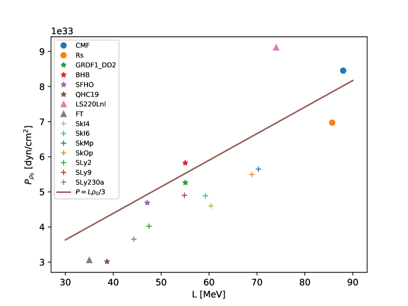
(a) Pressure in the neighborhood of the nuclear saturation density vs the slope parameter of the symmetry energy for a set of EoS in colored geometric shapes. The brown line represents Eq. (4).

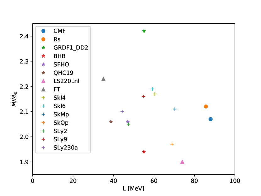
(b) Maximum mass vs the slope parameter of the symmetry energy for a set of EoS in colored geometric shapes.

Figure 1: Pressure and maximum mass vs the slope parameter of the symmetry energy.

In Fig. 1(a) we show a set of EoS for an energy range 30–90 MeV of the slope of the symmetry energy. For symmetric nuclear matter, the slope of the symmetry energy, $L$, is closely related to the pressure by means of

$$p\approxeq\frac{1}{3}L\rho_{0},$$ (4)

where $\rho_{0}$ is the nuclear saturation density. We can clearly observe a correlation in the vicinity of the nuclear saturation density. These EoS can be used in Eq. (2) and one can obtain the corresponding masses and radii. For Fig. 1(b) we considered the maximum mass that each EoS can reach. These stars have an associated $\rho_{c}$ (or $p_{c}$) that unlike $\rho_{0}$ cannot be reached on Earth, and the only way to determine stellar values is through an indirect method, i.e., through the maximum mass that one needs to compare with the observational data. No simple and direct correlation is seen in Fig. 1(b), as it was clear in the case of Fig. 1(a), for what one needs machine learning techniques that are robust to changes in complex correlations and the emergence of structures in global properties. Here, we are going to use a classification scheme, i.e., clustering techniques that will help us to make new predictions in future studies.

3 Clustering

Clustering methods were developed to study complex datasets and determine patterns and correlations among the degrees of freedom of the system (features). The idea is to separate the elements into groups that share similarities, often too complicated to be identified at first glance. The method of clustering falls into the category of unsupervised learning techniques [25].

To compute correlations, find global structures, and clusters, we consider a larger set of EoS than our previous work [8], where we were interested in the microscopic aspects. For this work, we use the 65 EoS from the LIGO Lalsuite [26] library. In Fig. 2 we show the maximum mass for all the EoS. We also show the possible region for the mass-radius according to the gravitational wave observation [21, 22] in a gray shaded circle. The horizontal dotted line marks two solar masses, since some pulsars above two solar masses have being observed [27, 28, 29, 30].

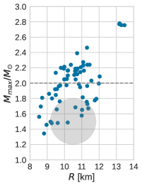
Figure 2: Maximum mass and its respective radius for 65 EoS from the LIGO Lalsuite [26] library. The gray shaded circle shows the mass-radius constraints from GW170817 event. The horizontal dotted line at $2\ M_{\odot}$ is to remind the two massive pulsars J0348+0432 and J1614-2230 observed.

$k$-means

Here we employed the $k$-means clustering method [25] to determine cluster structures present in the results shown in Fig.2. The $k$ is the number of $k$-means clusters present in the data set. This is a method of quantization [31, 25], where it assumes that the clusters are defined by the distance of the points to their class centers only. The goal of clustering is to find the $k$-mean vectors $c_{1},\ldots,c_{k}$ and provide the cluster assignment $y_{i}\in\{1,...,k\}$ of each point $x_{i}$ in the set. The following criterion is used:

$${\rm J}=\sum_{j=1}^{k}\sum_{i=j}^{n}\|x_{i}-c_{j}\|^{2}=\underset{\mathbf{S}}{\arg\min}\sum_{i=1}^{K}\left|S_{i}\right|\operatorname{Var}S_{i},$$ (5)

where centroids are given by: $c_{j}=\frac{1}{m_{j}}\sum_{i=1}^{m_{j}}x_{i}$.

In this way, given the initial set, the algorithm goes between two steps: (i) Assignment step: Assign one element to the cluster with the nearest mean with the least squared Euclidean distance; (ii) Update step: Recalculate the centroids for the elements of each cluster. The $k$-means algorithm is based on an interleaving approach where the cluster assignments $y_{i}$ are established given the centers and the centers are then computed given the assignments.

The number of $k$ clusters is determined with the help of well-known procedures [32, 25]. We have used two different ways to arrive and confirm the value of three clusters ($k=3$). The first one is the elbow point, which determines the $k$ and the homogeneity of the groups. On the left side of Fig. 3 we plot the within-group homogeneity as a function of $k$. The “elbow point” (vertical dashed line) represents the optimal for $k=3$ clusters. On the right side of the same Fig.3 we have the silhouette plot, which measures the similarity/cohesion of the elements to its clusters relative to other clusters employing a distance metric map. The optimal value here is found at the highest inflection point that takes place at $k=3$, which confirms the number of three cluster present in our data set. More details about methods employed here can be found in [25].

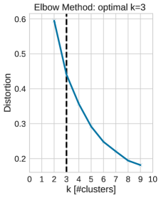
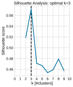
Figure 3: The Elbow and Silhouette methods to determine the optimal number of $k=3$ clusters.

In Fig. 4 (left panel), we show the resulting $k=3$ cluster structure obtained with the $k$-means approach. The three groups determined in this dataset are highlighted in different colors: the first one is pink, the second one in green and finally the third one in red. The dark stars give the position of each cluster centroid. Each cluster contains many EoS with different microphysical characteristics. The separation into groups represents similarities in traits or characteristics in this space $W$. On the right side of the same figure, we have the normalized stiffness of the EoS, we have the increment in the mass that goes from the softness to the stiff ones, the stiff EoS being responsible for the most massive stars. The clusters depicted by the $k$-means approach can be associated to three regimes of the stiffness space, the high (red), intermediate (green) and low (purple) regimes.

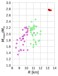
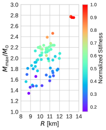
Figure 4: Left side: Three clusters obtained in the maximum mass and its respective radius space utilizing $k$-means. Right side: Mass-radius distribution according to the normalized stiffness of the EoS.

4 Concluding remarks

In this work, we have studied properties of a set of different EoS. We have solved the hydrostatic equilibrium equations to obtain the maximum mass and radius for each EoS. The outputs were used to define a vector space named $W$. The elements of this vector are taken to represent global characteristics of the microphysics of the equation of state for each model. Utilizing the $k$-means algorithm we were able to find structures in this space, leading to three subspaces, i.e. three clusters. The structures found represent similarities in traits/characteristics within the group only based in the elements of $W$. The number of clusters $k=3$ was determined with two different approaches frequently employed in ML studies. The resulting structures can be associated to differences in the physics models used to derive each EoS. We have shown that the clusters found by the unsupervised ML approach can be associated to different stiffness of the equation of state. We believe that this approach can be combined with astronomical data to find additional correlations. This would help for a better understanding of extrapolation limits of current models.

This work is a complementary study to our previous work [8], where we have analyzed the microphysics of the EoS. Combining the two works we can also study the $V\otimes W$ space which will certainly bring new correlations and bring light to the path of the correct EoS of neutron stars. We recall that the study of the whole M-R relation points is also important when comparing with precise data from LIGO-VIRGO-KAGRA and NICER and other astronomical data.

References

References

- [1] Haensel P, Potekhin A Y and Yakovlev D G 2007 Neutron Stars 1: Equation of State and Structure Astrophysics and Space Science Library, Neutron Stars (New York: Springer-Verlag) ISBN 978-0-387-33543-8
- [2] Margalit B and Metzger B D 2017 The Astrophysical Journal Letters 850 L19
- [3] Radice D, Perego A, Zappa F and Bernuzzi S 2018 The Astrophysical Journal Letters 852 L29
- [4] Tews I, Margueron J and Reddy S 2018 Physical Review C 98 045804
- [5] Motta T F, Kalaitzis A M, Antić S, Guichon P A M, Stone J R and Thomas A W 2019 The Astrophysical Journal 878 159
- [6] Gamba R, Read J S and Wade L E 2019 Classical and Quantum Gravity 37 025008
- [7] Lourenço O, Dutra M, Lenzi C H, Biswal S K, Bhuyan M and Menezes D P 2020 The European Physical Journal A 56 32
- [8] Lobato R V, Chimanski E V and Bertulani C A 2022 arXiv:2202.13940 [astro-ph, physics:nucl-th] (Preprint 2202.13940)
- [9] Lattimer J M and Prakash M 2001 The Astrophysical Journal 550 426–442
- [10] Lackey B D, Nayyar M and Owen B J 2006 Physical Review D 73 024021
- [11] Bejger M, Bulik T and Haensel P 2005 Monthly Notices of the Royal Astronomical Society 364 635–639
- [12] Özel F and Freire P 2016 Annual Review of Astronomy and Astrophysics 54 401–440
- [13] Glasko V B 1984 Inverse Problems of Mathematical Physics (American Institute of Physics)
- [14] Prilepko A I, Orlovsky D G and Vasin I A 2000 Methods for Solving Inverse Problems in Mathematical Physics (CRC Press) ISBN 978-0-8247-1987-6
- [15] Samarskii A A and Vabishchevich P N 2008 Numerical Methods for Solving Inverse Problems of Mathematical Physics (Walter de Gruyter) ISBN 978-3-11-020579-4
- [16] Aster R C, Borchers B and Thurber C H 2018 Parameter Estimation and Inverse Problems (Elsevier) ISBN 978-0-12-813423-8
- [17] Fujimoto Y, Fukushima K and Murase K 2018 Physical Review D 98 023019
- [18] Tolman R C 1939 Physical Review 55 364–373
- [19] Oppenheimer J R and Volkoff G M 1939 Physical Review 55 374–381
- [20] Reed B T, Fattoyev F J, Horowitz C J and Piekarewicz J 2021 Physical Review Letters 126 172503
- [21] The LIGO Scientific Collaboration and the Virgo Collaboration and et al 2018 Physical Review Letters 121 161101 (Preprint 1805.11581)
- [22] LIGO Scientific Collaboration and Virgo Collaboration and et al 2019 Physical Review X 9 011001 (Preprint 1805.11579)
- [23] Miller M C, Lamb F K, Dittmann A J, Bogdanov S, Arzoumanian Z, Gendreau K C, Guillot S, Harding A K, Ho W C G, Lattimer J M, Ludlam R M, Mahmoodifar S, Morsink S M, Ray P S, Strohmayer T E, Wood K S, Enoto T, Foster R, Okajima T, Prigozhin G and Soong Y 2019 The Astrophysical Journal 887 L24
- [24] Riley T E, Watts A L, Bogdanov S, Ray P S, Ludlam R M, Guillot S, Arzoumanian Z, Baker C L, Bilous A V, Chakrabarty D, Gendreau K C, Harding A K, Ho W C G, Lattimer J M, Morsink S M and Strohmayer T E 2019 The Astrophysical Journal 887 L21
- [25] Géron A 2017 Hands-on Machine Learning with Scikit-Learn and TensorFlow: Concepts, Tools, and Techniques to Build Intelligent Systems (O’Reilly Media) ISBN 978-1-4919-6229-9
- [26] LIGO Scientific Collaboration 2018 LIGO Algorithm Library - LALSuite free software (GPL)
- [27] Demorest P B, Pennucci T, Ransom S M, Roberts M S E and Hessels J W T 2010 Nature 467 1081–1083
- [28] Antoniadis J, Freire P C C, Wex N, Tauris T M, Lynch R S, van Kerkwijk M H, Kramer M, Bassa C, Dhillon V S, Driebe T, Hessels J W T, Kaspi V M, Kondratiev V I, Langer N, Marsh T R, McLaughlin M A, Pennucci T T, Ransom S M, Stairs I H, van Leeuwen J, Verbiest J P W and Whelan D G 2013 Science 340 1233232
- [29] Linares M, Shahbaz T and Casares J 2018 The Astrophysical Journal 859 54
- [30] Cromartie H T, Fonseca E, Ransom S M, Demorest P B, Arzoumanian Z, Blumer H, Brook P R, DeCesar M E, Dolch T, Ellis J A, Ferdman R D, Ferrara E C, Garver-Daniels N, Gentile P A, Jones M L, Lam M T, Lorimer D R, Lynch R S, McLaughlin M A, Ng C, Nice D J, Pennucci T T, Spiewak R, Stairs I H, Stovall K, Swiggum J K and Zhu W W 2020 Nature Astronomy 4 72–76
- [31] Linde Y, Buzo A and Gray R 1980 IEEE Transactions on Communications 28 84–95
- [32] Halkidi M, Batistakis Y and Vazirgiannis M 2001 Journal of Intelligent Information Systems 17 107–145