Shape-Pose Disentanglement using $\mathbf{SE}(3)$-equivariant Vector Neurons

Abstract.

We introduce an unsupervised technique for encoding point clouds into a canonical shape representation, by disentangling shape and pose. Our encoder is stable and consistent, meaning that the shape encoding is purely pose-invariant, while the extracted rotation and translation are able to semantically align different input shapes of the same class to a common canonical pose. Specifically, we design an auto-encoder based on Vector Neuron Networks, a rotation-equivariant neural network, whose layers we extend to provide translation-equivariance in addition to rotation-equivariance only. The resulting encoder produces pose-invariant shape encoding by construction, enabling our approach to focus on learning a consistent canonical pose for a class of objects. Quantitative and qualitative experiments validate the superior stability and consistency of our approach.

1. Introduction

Point clouds reside at the very core of 3D geometry processing, as they are acquired at the beginning of the 3D processing pipeline and usually serve as the raw input for shape analysis or surface reconstruction. Thus, understanding the underlying geometry of a point cloud has a profound impact on the entire 3D processing chain. This task, however, is challenging since point clouds are unordered, and contain neither connectivity, nor any other global information.

In recent years, with the emergence of neural networks, various techniques have been developed to circumvent the challenges of analyzing and understanding point clouds [Qi et al., 2017a, b; Wang et al., 2019; Hamdi et al., 2021; Ma et al., 2022; Shi et al., 2019; Liu et al., 2020; Yang et al., 2020]. However, most methods rely on pre-aligned datasets, where the point clouds are normalized, translated and oriented to have the same pose.

In this work, we present an unsupervised technique to learn a canonical shape representation by disentangling shape, translation, and rotation. Essentially, the canonical representation is required to meet two conditions: stability and consistency. The former means that the shape encoding should be invariant to any rigid transformation of the same input, while the latter means that different shapes of the same class should be semantically aligned, sharing the same canonical pose.

Canonical alignment is not a new concept. Recently, Canonical Capsules [Sun et al., 2021] and Compass [Spezialetti et al., 2020] proposed self-supervised learning of canonical representations using augmentations with Siamese training. We discuss these methods in more detail in the next section. In contrast, our approach is to extract a pose-invariant shape encoding, which is explicitly disentangled from the separately extracted translation and rotation.

Specifically, we design an auto-encoder, trained on an unaligned dataset, that encodes the input point cloud into three disentangled components: (i) a pose-invariant shape encoding, (ii) a rotation matrix and (iii) a translation vector. We achieve pure $\mathbf{SE}(3)$-invariant shape encoding and $\mathbf{SE}(3)$-equivariant pose estimation (enabling reconstruction of the input shape), by leveraging a novel extension of the recently proposed Vector Neuron Networks (VNN) [Deng et al., 2021]. The latter is an $\mathbf{SO}(3)$-equivariant neural network for point cloud processing, and while translation invariance could theoretically be achieved by centering the input point clouds, such approach is sensitive to noise, missing data and partial shapes. Therefore we propose an extension to VNN achieving $\mathbf{SE}(3)$-equivariance.

It should be noted that the shape encodings produced by our network are stable (i.e., pose-invariant) by construction, due to the use of $\mathbf{SE}(3)$-invariant layers.

At the same time, the extracted rigid transformation is equivariant to the pose of the input. This enables the learning process to focus on the consistency across different shapes. Consistency is achieved by altering the input point cloud with a variety of simple shape augmentations, while keeping the pose fixed, allowing us to constrain the learned transformation to be invariant to the identity, (i.e., the particular shape), of the input point cloud.

Moreover, our disentangled shape and pose representation is not limited to point cloud decoding, but can be combined with any 3D data decoder, as we demonstrate by learning a canonical implicit representation of our point cloud utilizing occupancy networks [Mescheder et al., 2019].

We show, both qualitatively and quantitatively, that our approach leads to a stable, consistent, and purely $\mathbf{SE}(3)$-invariant canonical representation compared to previous approaches.

2. Background and Related Work

2.1. Canonical representation

A number of works proposed techniques to achieve learnable canonical frames, typically requiring some sort of supervision [Rempe et al., 2020; Novotny et al., 2019; Gu et al., 2020]. Recently, two unsupervised methods were proposed: Canonical Capsules [Sun et al., 2021] and Compass [Spezialetti et al., 2020]. Canonical Capsules [Sun et al., 2021] is an auto-encoder network that extracts positions and pose-invariant descriptors for $k$ capsules, from which the input shape may be reconstructed. Pose invariance and equivariance are achieved only implicitly via Siamese training, by feeding the network with pairs of rotated and translated versions of the same input point cloud.

Compass [Spezialetti et al., 2020] builds upon spherical CNN [Cohen et al., 2018], a semi-equivariant $\mathbf{SO}(3)$ network, to estimate the pose with respect to the canonical representation. It should be noted that Compass is inherently tied to spherical CNN, which is not purely equivariant [Cohen et al., 2018]. Thus, similarly to Canonical Capsules, Compass augments the input point cloud with a rotated version to regularize an equivariant pose estimation. It should be noted that neither method guarantees pure equivariance.

Similarly to Canonical Capsules, we employ an auto-encoding scheme to disentangle pose from shape, i.e., the canonical representation, and similarly to Compass, we strive to employ an equivariant network, however, our network is $\mathbf{SE}(3)$-equivariant and not only $\mathbf{SO}(3)$-equivariant. More importantly, differently from these two approaches, the different branches of our network are $\mathbf{SE}(3)$-invariant or $\mathbf{SE}(3)$-equivariant by construction, and thus the learning process is free from the burden of enforcing these properties. Rather, the process focuses on learning a consistent shape representation in a canonical pose.

2.2. 3D reconstruction

Our method reconstructs an input point cloud by disentangling the input 3D geometry into shape and pose. The encoder outputs a pose encoding and a shape encoding which is pose-invariant by construction, while the decoder reconstructs the 3D geometry from the shape encoding alone. Consequently, our architecture can be easily integrated into various 3D auto-encoding pipelines. In this work, we shall demonstrate our shape-pose disentanglement for point cloud encoding and implicit representation learning.

State-of-the-art point cloud auto-encoding methods rely on a folding operation of a template (optionally learned) hyperspace point cloud to the input 3D point cloud [Yang et al., 2018; Groueix et al., 2018; Deprelle et al., 2019]. Following this approach, we employ AtlasNetV2 [Deprelle et al., 2019] which uses multiple folding operations from hyperspace patches to 3D coordinates, to reconstruct point clouds in a pose-invariant frame.

Implicit 3D representation networks [Mescheder et al., 2019; Park et al., 2019; Xu et al., 2019] enable learning of the input geometry with high resolution and different mesh topology. We utilize occupancy networks [Mescheder et al., 2019] to learn an implicit pose-invariant shape representation.

2.3. Rotation-equivariance and Vector Neuron Network

The success of 2D convolutional neural networks (CNN) on images, which are equivariant to translation, drove a similar approach for 3D data with rotation as the symmetry group. The majority of works on 3D rotation-equivariance [Esteves et al., 2018; Cohen et al., 2018; Thomas et al., 2018; Weiler et al., 2018], focus on steerable CNNs [Cohen and Welling, 2016], where each layer “steers” the output features according to the symmetry property (rotation and occasionally translation for 3D data). For example, Spherical CNNs [Esteves et al., 2018; Cohen et al., 2018] transform the input point cloud to a spherical signal, and use spherical harmonics filters, yielding features on $\mathbf{SO}(3)$-space. Usually, these methods are tied with specific architecture design and data input which limit their applicability and adaptation to SOTA 3D processing.

Recently, Deng et al. [Deng et al., 2021] introduced Vector Neuron Networks (VNN), a rather light and elegant framework for $\mathbf{SO}(3)$-equivariance. Empirically, the VNN design performs on par with more complex and specific architectures. The key benefit of VNNs lies in their simplicity, accessibility and generalizability. Conceptually, any standard point cloud processing network can be elevated to $\mathbf{SO}(3)$-equivariance (and invariance) with minimal changes to its architecture. Below we briefly describe VNNs and refer the reader to [Deng et al., 2021] for further details.

In VNNs the representation of a single neuron is lifted from a sequence of scalar values to a sequence of 3D vectors. A single vector neuron feature is thus a matrix $\mathbb{V}\in\mathbb{R}^{C\times 3}$, and we denote a collection of $N$ such features by $\mathcal{V}\in\mathbb{R}^{N\times C\times 3}$. The layers of VNNs, which map between such collections, $f:\mathcal{V}\in\mathbb{R}^{N\times C\times 3}\rightarrow\mathbb{\mathcal{V}^{\prime}}\in\mathbb{R}^{N\times C^{\prime}\times 3}$, are equivariant to rotations $R\in\mathbb{R}^{3\times 3}$, that is:

(1) $$f\left(\mathcal{V}R\right)=f\left(\mathbb{\mathcal{V}}\right)R,$$

where $\mathcal{V}R=\left\{\mathbb{V}_{n}R\right\}_{n=1}^{N}$.

Ordinary linear layers fulfill this requirement, however, other non-linear layers, such as ReLU and max-pooling, do not. For ReLU activation, VNNs apply a truncation w.r.t to a learned half-space. Let $\mathbb{V},\mathbb{V^{\prime}}\in\mathbb{R}^{C\times 3}$ be the input and output vector neuron features of a single point, respectively. Each 3D vector $\mathbb{v}^{\prime}\in\mathbb{V}^{\prime}$ is obtained by first applying two learned matrices $\mathbb{Q},\mathbb{K}\in\mathbb{R}^{1\times C}$ to project $\mathbb{V}$ to a feature $\mathbb{q}=\mathbb{Q}\mathbb{V}\in\mathbb{R}^{1\times 3}$ and a direction $\mathbb{k}=\mathbb{K}\mathbb{V}\in\mathbb{R}^{1\times 3}$. To achieve equivariance, $\mathbb{v}^{\prime}\in\mathbb{V^{\prime}}$ is then defined by truncating the part of $\mathbb{q}$ that lies in the negative half-space of $\mathbb{k}$, as follows,

(2) $$\mathbb{v^{\prime}}=\begin{cases}\mathbb{q}&\text{if}\quad{\left\langle\mathbb{q},\mathbb{k}\right\rangle}\geq 0,\\ \mathbb{q}-{\left\langle\mathbb{q},\frac{\mathbb{k}}{\left\lVert\mathbb{k}\right\rVert}\right\rangle}\frac{\mathbb{k}}{\left\lVert\mathbb{k}\right\rVert}&\text{otherwise}.\end{cases}$$

In addition, VNNs employ rotation-equivariant pooling operations and normalization layers. We refer the reader to [Deng et al., 2021] for the complete definition.

Invariance layers can be achieved by inner product of two rotation-equivariant features. Let $\mathbb{V}\in\mathbb{R}^{C\times 3}$, and $\mathbb{V^{\prime}}\in\mathbb{R}^{C^{\prime}\times 3}$ be two equivariant features obtained from an input point cloud $\mathbb{X}$. Then rotating $\mathbb{X}$ by a matrix $R$, results in the features $\mathbb{V}R$ and $\mathbb{V^{\prime}}R$, and

(3) $$\langle\mathbb{V}R,\mathbb{V^{\prime}}R\rangle=\mathbb{V}R(\mathbb{V^{\prime}}R)^{T}=\mathbb{V}RR^{T}\mathbb{V^{\prime}}^{T}=\mathbb{V}\mathbb{V^{\prime}}^{T}=\langle\mathbb{V},\mathbb{V^{\prime}}\rangle.$$

In our work, we also utilize vector neurons, but we extend the different layers to be $\mathbf{SE}(3)$-equivariant, instead of $\mathbf{SO}(3)$-equivariant, as described in Section 3.1. This new design allow us to construct an $\mathbf{SE}(3)$-invariant encoder, which gradually disentangles the pose from the shape, first the translation and then the rotation, resulting in a pose-invariant shape encoding.

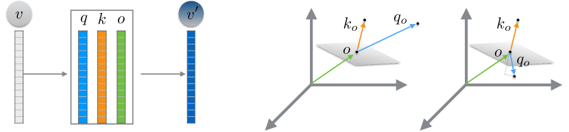
Figure 1. Vector Neuron Translation equivariant non linear layer. We learn for each input point feature $\mathbb{v}$, three component $\mathbb{o},\mathbb{q},\mathbb{k}$, and interpret them as an origin $\mathbb{o}$, a feature $\mathbb{q_{o}}=\mathbb{q}-\mathbb{o}$ and a direction $\mathbb{k_{o}}=\mathbb{k}-\mathbb{o}$. Similarly to VNN operation, the feature component of $\mathbb{q_{o}}$ which is in the half-space defined by $-\mathbb{k_{o}}$ is clipped. In-addition, we translate the feature by the learned origin $\mathbb{o}$ outputting the $\mathbb{v^{\prime}}$.

3. Method

We design an auto-encoder to disentangle shape, translation, and rotation. We wish the resulting representation to be stable, i.e., the shape encoding should be pose-invariant, and the pose $\mathbf{SE}(3)$-equivariant. At the same we wish multiple different shapes in the same class to have a consistent canonical pose. To achieve stability, we revisit VNNs and design new $\mathbf{SE}(3)$-equivariant and invariant layers, which we refer to as Vector Neurons with Translation (VNT). Consistency is then achieved by self-supervision, designed to preserve pose across shapes. In the following, we first describe the design of our new VNT layers. Next, we present our VNN and VNT-based auto-encoder architecture. Finally, we elaborate on our losses to encourage disentanglement of shape from pose in a consistent manner.

3.1. $\mathbf{SE}(3)$-equivariant Vector Neuron Network

As explained earlier, Vector Neuron Networks (VNN) [Deng et al., 2021] provide a framework for $\mathbf{SO}(3)$-equivariant and invariant point cloud processing. Since a pose of an object consists of translation and rotation, $\mathbf{SE}(3)$-equivariance and invariance are needed for shape-pose disentanglement. While it might seem that centering the input point cloud should suffice, note that point clouds are often captured with noise and occlusions, leading to missing data and partial shapes, which may significantly affect the global center of the input. Specifically, for canonical representation learning, a key condition is consistency across different objects, thus, such an approach assumes that the center of the point cloud is consistently semantic between similar but different objects, which is hardly the case. Equivariance to translation, on the other-hand, allows identifying local features in different locations with the same filters, without requiring global parameters.

Therefore, we revisit the Vector Neuron layers and extend them to Vector Neurons with Translation (VNT), thereby achieving $\mathbf{SE}(3)$-equivariance.

3.1.1. Linear layers:

While linear layers are by definition rotation-equivariant, they are not translation-equivariant. Following VNN, our linear module $f_{\textrm{lin}}\left(\cdot;\mathbb{W}\right)$ is defined via a weight matrix $\mathbb{W}\in\mathbb{R}^{C^{\prime}\times C}$, acting on a vector-list feature $\mathbb{V}\in\mathbb{R}^{C\times 3}$. Let $R\in\mathbb{R}^{3\times 3}$ be a rotation matrix and $T\in\mathbb{R}^{1\times 3}$ a translation vector. For $f_{\textrm{lin}}\left(\cdot;\mathbb{W}\right)$ to be $\mathbf{SE}(3)$-equivariant, the following must hold:

(4) $$f_{\textrm{lin}}\left(\mathbb{V}R+\mathbbm{1}_{C}T\right)=\mathbb{W}\mathbb{V}R+\mathbb{\mathbbm{1}}_{C^{\prime}}T=f_{\textrm{lin}}(\mathbb{V})R+\mathbb{\mathbbm{1}}_{C^{\prime}}T,$$

where $\mathbbm{1}_{C}=[1,1,\dots,1]^{T}\in\mathbb{R}^{C\times 1}$ is a column vector of length $C$. A sufficient condition for (18) to hold is achieved by constraining each row of $\mathbb{W}$ to sum to one. Formally, $\mathbb{W}\in\mathcal{W}^{C^{\prime}\times C}$, where

(5) $$\mathcal{W}^{C^{\prime}\times C}=\left\{\mathbb{W}\in\mathbb{R}^{C^{\prime}\times C}\mid\textstyle{\sum_{j=1}^{C}}w_{i,j}=1\quad\forall i\in[1,C^{\prime}]\right\},$$

See the supplementary material for a complete proof.

3.1.2. Non-linear layers:

We extend each non-linear VNN layer to become $\mathbf{SE}(3)$-equivariant by adding a learnable origin. More formally, for the ReLU activation layer, given an input feature list $\mathbb{V}\in\mathbb{R}^{C\times 3}$, we learn three (rather than two) linear maps, $\mathbb{Q},\mathbb{K},\mathbb{O}\in\mathcal{W}^{1\times C}$ projecting the input to $\mathbb{q},\mathbb{k},\mathbb{o}\in\mathbb{R}^{1\times 3}$. The feature and direction are defined w.r.t the origin $\mathbb{o}$, i.e., the feature is given by $\mathbb{q_{o}}=\mathbb{q}-\mathbb{o}$, while the direction is given by $\mathbb{k_{o}}=\mathbb{k}-\mathbb{o}$, as illustrated in Fig. 1. The ReLU is applied by clipping the part of $\mathbb{q_{o}}$ that resides behind the plane defined by $\mathbb{k_{o}}$ and $\mathbb{o}$, i.e.,

(6) $$\mathbb{v^{\prime}}=\begin{cases}\mathbb{o}+\mathbb{q_{o}}&\text{if}\quad{\left\langle\mathbb{q_{o}},\mathbb{k_{o}}\right\rangle}\geq 0,\\ \mathbb{o}+\mathbb{q_{o}}-{\left\langle\mathbb{q_{o}},\frac{\mathbb{k_{o}}}{\left\lVert\mathbb{k_{o}}\right\rVert}\right\rangle}\frac{\mathbb{k_{o}}}{\left\lVert\mathbb{k_{o}}\right\rVert},&\text{otherwise}.\end{cases},$$

Note that $\mathbb{o}+\mathbb{q_{o}}=\mathbb{q}$, and that $\mathbb{K},\mathbb{O}$ may be shared across the elements of $\mathbb{V}.$

It may be easily seen that we preserve the equivariance w.r.t $\mathbf{SO}(3)$ rotations, as well translations. In the same manner, we extend the $\mathbf{SO}(3)$-equivariant VNN maxpool layer to become $\mathbf{SE}(3)$-equivariant. We refer the reader to the supplementary material for the exact adaptation and complete proof.

3.1.3. Translation-invariant layers:

Invariance to translation can be achieved by subtracting two $\mathbf{SE}(3)$-equivariant features. Let $\mathbb{V},\mathbb{V^{\prime}}\in\mathbb{R}^{C\times 3}$ be two $\mathbf{SE}(3)$-equivariant features obtained from an input point cloud $\mathbb{X}$. Then, rotating $\mathbb{X}$ by a matrix $R$ and translating by $T$, results in the features $\mathbb{V}R+\mathbb{\mathbbm{1}}_{C}T$ and $\mathbb{V^{\prime}}R+\mathbb{\mathbbm{1}}_{C}T$, whose difference is translation-invariant:

(7) $$\left(\mathbb{V}R+\mathbb{\mathbbm{1}}_{C}T\right)-\left(\mathbb{V^{\prime}}R+\mathbb{\mathbbm{1}}_{C}T\right)=\left(\mathbb{V}-\mathbb{V^{\prime}}\right)R$$

Note that the resulting feature is still rotation-equivariant, which enables to process it with VNN layers, further preserving $\mathbf{SO}(3)$-equivariance.

3.2. $\mathbf{SE}(3)$-equivariant Encoder-Decoder

We design an auto-encoder based on VNT and VNN layers to disentangle pose from shape. Thus, our shape representation is pose-invariant (i.e., stable), while our pose estimation is $\mathbf{SE}(3)$-pose-equivariant, by construction. The decoder, which can be an arbitrary 3D decoder network, reconstructs the 3D shape from the invariant features.

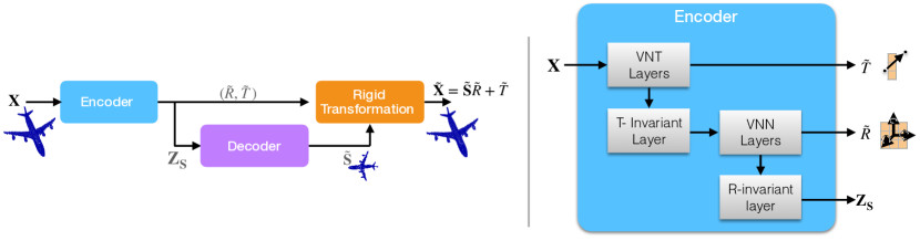
Figure 2. The architecture of our auto-encoder for shape-pose disentanglement. The auto-encoder (left) disentangles the input point cloud $\mathbb{X}$ to rotation $\tilde{R}$, translation $\tilde{T}$ and a canonical representation $\tilde{\mathbb{S}}$. The shape encoding $\mathbb{Z_{s}}$ is invariant by construction to the pose, while the learned rotation and translation are equivariant to it. Our encoder (right) learns features that are initially equivariant to the pose, and gradually become invariant to it, first to translation and then to rotation, eventually yielding pose invariant features $\mathbb{Z_{s}}$.

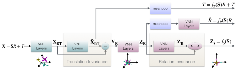
Figure 3. The architecture of our encoder. The representation of the input point cloud $\mathbb{X}$ yields a pose-invariant (bottom branch) shape encoding $\mathbb{Z_{s}}$ in two steps: first, making it invariant to translation and then to rotation. At the same time, the learned rigid transformation $(\tilde{R},\tilde{T})$ (top and middle branches) is equivariant to the input pose. The small rendered planes at the bottom, illustrate the alignment at each stage.

The overall architecture of our AE is depicted in Fig. 2. Given an input point cloud $\mathbb{X}\in\mathbb{R}^{N\times 3}$, we can represent it as a rigid transformation of an unknown canonical representation $\mathbb{S}\in\mathbb{R}^{N\times 3}$:

(8) $$\mathbb{X}=\mathbb{S}R+\mathbbm{1}_{N}T,$$

where $\mathbbm{1}_{N}=[1,1,\dots,1]^{T}\in\mathbb{R}^{N\times 1}$ is a column vector of length $N$, $R\in\mathbb{R}^{3\times 3}$ is a rotation matrix and $T\in\mathbb{R}^{1\times 3}$ is a translation vector.

Our goal is to find the shape $\mathbb{S}$, which is by definition pose-invariant and should be consistently aligned across different input shapes. To achieve this goal, we use an encoder that first estimates the translation $\tilde{T}$ using translation-equivariant VNT layers, then switches to a translation-invariant representation from which the rotation $\tilde{R}$ is estimated using rotation-equivariant VNN layers. Finally, the representation is made rotation-invariant and the shape encoding $\mathbb{Z_{s}}$ is generated. A reconstruction loss is computed by decoding $\mathbb{Z_{s}}$ into the canonically-positioned shape $\tilde{\mathbb{S}}$ and applying the extracted rigid transformation. In the following we further explain our encoder architecture and the type of decoders used.

3.2.1. $\mathbf{SE}(3)$-equivariant Encoder

Our encoder is composed of rotation and translation equivariant and invariant layers as shown in Fig. 3. We start by feeding $\mathbb{X}$ through linear and non-linear VNT layers yielding $\mathbb{X_{RT}}\in\mathbb{R}^{N\times C\times 3}$, where the $RT$ subscript indicates $\mathbf{SE}(3)$-equivariant features, as described in Section 3.1.

$\mathbb{X_{RT}}$ is then fed-forward through additional VNT layers resulting in a single vector neuron per point $\mathbb{\bar{X}_{RT}}\in\mathbb{R}^{N\times 1\times 3}$. We mean-pool the features to produce a 3D SE(3)-equivariant vector as our translation estimation, as shown in the upper branch of Fig. 3, yielding $\tilde{T}=f_{T}(\mathbb{X})=f_{T}(\mathbb{S})R+T\in\mathbb{R}^{1\times 3}$, where we denote by $f_{T}:\mathbb{R}^{N\times 3}\rightarrow\mathbb{R}^{1\times 3}$ the aggregation of the VNT-layers from the input point cloud $\mathbb{X}$ to the estimated $\tilde{T}$, thus, it is a translation and rotation equivariant network.

In addition, as explained in Section 3.1, the following creates translation invariant features, $\mathbb{Y_{R}}=\mathbb{X_{RT}}-\mathbb{\bar{X}_{RT}}\in\mathbb{R}^{N\times C\times 3}$.

While $\mathbb{Y_{R}}$ is translation invariant, it is still rotation equivariant, thus, we can proceed to further process $\mathbb{Y_{R}}$ with VNN layers, resulting in (deeper) rotation equivariant features $\mathbb{Z_{R}}\in\mathbb{R}^{N\times C^{\prime}\times 3}$.

Finally, $\mathbb{Z_{R}}$ is fed forward through a VNN rotation-invariant layer as explained in Section 2.3, resulting in a shape encoding, $\mathbb{Z_{s}}$, which is by construction pose invariant. Similar to the translation reconstruction, the rotation is estimated by mean pooling $\mathbb{Z_{R}}$ and feeding it through a single VN linear layer yielding $\tilde{R}=f_{R}(\mathbb{X})=f_{R}(\mathbb{S})R\in\mathbb{R}^{3\times 3},$

where $f_{R}:\mathbb{R}^{N\times 3}\rightarrow\mathbb{R}^{3\times 3}$ denotes the aggregation of the layers from the input point cloud $\mathbb{X}$ to the estimated rotation $\tilde{R}$ and, as such, it is a rotation-equivariant network. The entire encoder architecture is shown in Fig. 3 and we refer the reader to our supplementary for a detailed description of the layers.

3.2.2. Decoder

The decoder is applied on the shape encoding $\mathbb{Z_{s}}$ to reconstruct the shape $\tilde{\mathbb{S}}$. We stress again that $\tilde{\mathbb{S}}$ is invariant to the input pose, regardless of the training process. Motivated by the success of folding networks [Yang et al., 2018; Groueix et al., 2018; Deprelle et al., 2019] for point clouds auto-encoding, we opt to use AtlasNetV2 [Deprelle et al., 2019] as our decoder, specifically using the point translation learning module. For implicit function reconstruction, we follow Occupancy network decoder [Mescheder et al., 2019]. Please note, that our method is not coupled with any decoder structure.

3.3. Optimizing for shape-pose disentanglement

While our auto-encoder is pose-invariant by construction, the encoding has no explicit relation to the input geometry. In the following we detail our losses to encourage a rigid relation between $\tilde{\mathbb{S}}$ and $X$, and for making $\tilde{\mathbb{S}}$ consistent across different objects.

3.3.1. Rigidity

To train the reconstructed shape $\mathbb{\tilde{S}}$ to be isometric to the input point cloud $\mathbb{X}$, we enforce a rigid transformation between the two, namely ${\mathbb{X}=\mathbb{\tilde{S}}\tilde{R}+\mathbbm{1}_{N}\tilde{T}}$.

For point clouds auto-encoding we have used the Chamfer Distance (CD):

(9) $$\mathcal{L}_{\textit{rec}}=\textit{CD}\left(\mathbb{X},\mathbb{\tilde{S}}\tilde{R}+\mathbbm{1}_{N}\tilde{T}\right),$$

Please note that other tasks such as implicit function reconstruction use equivalent terms, as we detail in our supplementary files.

In addition, while $\tilde{R}=f_{R}(\mathbb{X})$ is rotation-equivariant we need to constraint it to SO(3), and we do so by adding an orthonormal term:

(10) $$\mathcal{L}_{\textit{ortho}}=\|I-\tilde{R}\tilde{R}^{T}\|^{2}_{2}+\|I-\tilde{R}^{T}\tilde{R}\|_{2}^{2},$$

where $\|\cdot\|_{2}$ is mean square error (MSE) loss.

3.3.2. Consistency

Now, our shape reconstruction $\mathbb{\tilde{S}}$ is isometric to $\mathbb{X}$ and it is invariant to $T$ and $R$. However, there is no guarantee that the pose of $\mathbb{\tilde{S}}$ would be consistent across different instances.

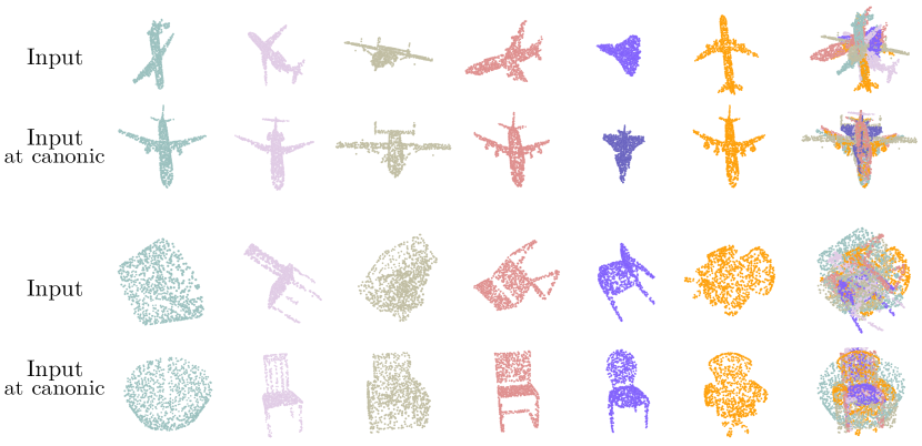
Figure 4. Aligning planes and chairs. The input planes and chairs (first and third row, respectively) have different shapes and different poses, as can be seen separately and together (rightmost column). We apply the inverse learned pose, transforming the input to its canonical pose (second and fourth row).

Assume two different point clouds $\mathbb{X_{1}},\mathbb{X_{2}}$ are aligned. If their canonical representations $\mathbb{S_{1}},\mathbb{S_{2}}$ are also aligned, then they have the same rigid transformation w.r.t their canonical representation and vice versa, i.e., $\mathbb{X_{i}}=\mathbb{S_{i}}R+\mathbbm{1}_{N}T$, $i=1,2$. To achieve such consistency, we require:

(11) $$\{f_{T}(\mathbb{X_{1}}),f_{R}(\mathbb{X_{1}})\}=\{f_{T}(\mathbb{X_{2}}),f_{R}(\mathbb{X_{2}})\}.$$

We generate such pairs of aligned point clouds, by augmenting the input point cloud $\mathbb{X}$ with several simple augmentation processes, which do not change the pose of the object. In practice, we have used Gaussian noise addition, furthest point sampling (FPS), patch removal by k-nn (we select one point randomly and remove $k$ of its nearest neighbors) and re-sampling of the input point cloud.

We then require that the estimated rotation and translation is the same for the original and augmented versions,

(12) $$\mathcal{L}^{\textit{aug}}_{\textit{consist}}=\sum_{A\in\mathcal{A}}\|f_{R}\left(\mathbb{X}\right)-f_{R}\left(A(\mathbb{X})\right)\|_{2}^{2}+\|f_{T}\left(\mathbb{X}\right)-f_{T}\left(A(\mathbb{X})\right)\|_{2}^{2},$$

where $\mathcal{A}$ is the group of pose preserving augmentations and $\|\cdot\|_{2}$ is MSE loss.

In addition, for point cloud reconstruction, we can also generate a version of $\mathbb{X}$, with a known pose, by feeding again the reconstructed shape $\mathbb{\tilde{S}}$. We transform $\mathbb{\tilde{S}}$ by a random rotation matrix $R^{*}$ and a random translation vector $T^{*}$ and require the estimated pose to be consistent with this transformation:

(13) $$\mathcal{L}^{\textit{can}}_{\textit{consist}}=\|f_{R}\left(\mathbb{\tilde{S}}R^{*}+T^{*}\right)-R^{*}\|_{2}^{2}+\|f_{T}\left(\mathbb{\tilde{S}}R^{*}+T^{*}\right)-T^{*}\|_{2}^{2},$$

Our overall loss is

(14) $$\mathcal{L}=\mathcal{L}_{\textit{rec}}+\lambda_{1}\mathcal{L}_{\textit{ortho}}+\lambda_{2}\mathcal{L}^{\textit{aug}}_{\textit{consist}}+\lambda_{3}\mathcal{L}^{\textit{can}}_{\textit{consist}},$$

where the $\lambda_{i}$ are hyper parameters, whose values in all our experiments were set to $\lambda_{1}=0.5$, $\lambda_{2}=\lambda_{3}=1$.

3.4. Inference

At inference time, we feed forward point cloud $\mathbb{X}\in\mathbb{R}^{N\times 3}$ and retrieve its shape and pose. However, since our estimated rotation matrix $\tilde{R}$ is not guaranteed to be orthonormal, at inference time, we find the closest ortho-normal matrix to $\tilde{R}$ (i.e., minimize the Forbenius norm), following [Bar-Itzhack, 1975], by solving:

(15) $$\hat{R}=\tilde{R}\left(\tilde{R}^{T}\tilde{R}\right)^{-\frac{1}{2}}.$$

The inverse of the square root can be computed by singular value decomposition (SVD). While this operation is also differentiable we have found it harmful to incorporate this constraint during the training phase, thus it is only used during inference. We refer the reader to [Bar-Itzhack, 1975] for further details.

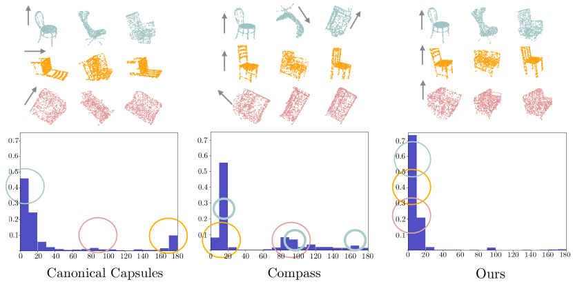
Figure 5. Histogram of canonical pose deviation from the mean canonical pose. We estimate the canonical pose of aligned 3D point clouds from ShapeNet using our method, Canonical Capsules [Sun et al., 2021] and Compass [Spezialetti et al., 2020]. In the bottom row, we show the normalized histogram of the deviation from the mean pose. It is clear that while our method is shape-consistent, both Compass and Canonical Capsules struggle to have a single canonical pose. In the top row, we focus on small, medium and large deviation cases of Canonical Capsules, marked by cyan, red, and orange circles on the histogram plot, respectively. The canonical pose of the same objects is shown for Compass and our method, as well as their location on the corresponding histogram plot. The arrow next to the objects is directed toward the local shape z+ direction.

4. Results

We preform qualitative and quantitative comparison of our method for learning shape-invariant pose. Due to page limitations, more results can be found in our supplementary files.

4.1. Dataset and implementation details

We employ the ShapeNet dataset [Chang et al., 2015] for evaluation. For point cloud auto-encoding we follow the settings in [Sun et al., 2021] and [Deprelle et al., 2019], and use ShapeNet Core focusing on two categories: airplanes and chairs. While airplanes are more semantically consistent and containing less variation, chairs exhibit less shape-consistency and may contain different semantic parts. All 3D models are randomly rotated and translated in the range of $[-0.1,0.1]$ at train and test time.

For all experiments, unless stated otherwise, we sample random $1024$ points for each point cloud. The auto-encoder is trained using Adam optimizer with learning rate of $1e^{-3}$ for $500$ epochs, with drop to the learning rate at $250$ and $350$ by a factor of $10$. We save the last iteration checkpoint and use it for our evaluation. The decoder is AtlasNetV2 [Deprelle et al., 2019] decoder with $10$ learnable grids.

4.2. Pose consistency

We first qualitatively evaluate the consistency of our canonical representation as shown in Fig. 4. At test time, we feed different instances at different poses through our trained network, yielding estimated pose of the input object w.r.t the pose-invariant shape. We then apply the inverse transformation learned, to transform the input to its canonical pose. As can be seen, the different instances are roughly aligned, despite having different shapes. More examples can be found in our supplementary files.

We also compare our method, both qualitatively and quantitatively, to Canonical Capsules [Sun et al., 2021] and Compass [Spezialetti et al., 2020] by using the alignment in ShapeNet (for Compass no translation is applied). First, we feed forward all of the aligned test point clouds $\left\{\mathbb{X}_{i}\right\}_{i=1}^{N_{t}}$ through all methods and estimate their canonical pose $\{\tilde{R}_{i}\}_{i=1}^{N_{t}}$. We expect to have a consistent pose for all aligned input shapes, thus, we quantify for each instance $i$ the angular deviation $d^{\textit{consist}}_{i}$ of its estimated pose $\tilde{R}_{i}$ from the mean pose $d^{\textit{consist}}_{i}=\angle{\left(\tilde{R}_{i},\frac{1}{N_{t}}\sum_{i}\tilde{R}_{i}\right)}.$ We present an histogram of $\{d^{\textit{consist}}_{i}\}_{i=1}^{N_{t}}$ in Fig. 5. As can be seen, our method results in a more aligned canonical shapes as indicated by the peak around the lower deviation values. We visualize the misalignment of Canonical Capsules by sampling objects with small, medium and large deviation, and compare them to the canonical representation achieved by Compass and our method for the same instances. The misalignment of Canonical Capsules may be attributed to the complexity of matching unsupervised semantic parts between chairs as they exhibit high variation (size, missing parts, varied structure). We quantify the consistency by the standard deviation of the estimated pose $\sqrt{\frac{1}{N_{t}}\sum_{i}{d_{i}^{2}}}$ in Table 1. Evidently, Compass falls short for both object classes. Canonical Capsules preform slightly better than our method for planes, while our method is much more consistent for the chair category.

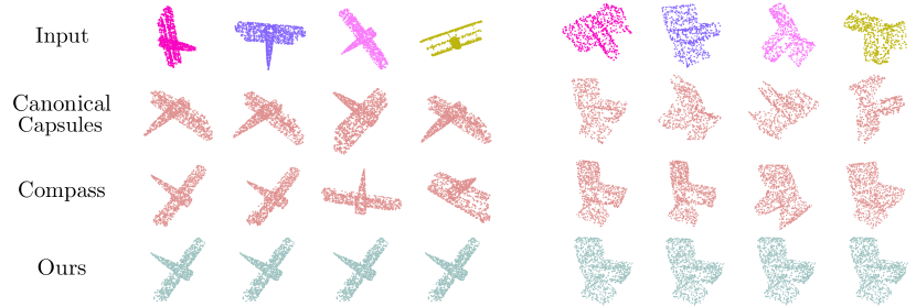
Figure 6. Stability of the canonical representation to rigid transformation of the input. The location and orientation of the same point cloud affects its canonical representation in both Canonical Capsules [Sun et al., 2021] and Compass [Spezialetti et al., 2020]. Our canonical representation (bottom row) is $\mathbf{SE}(3)$-invariant to the rigid transformation of the input.

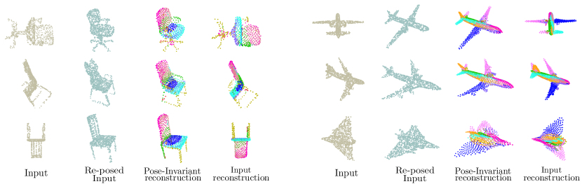
Figure 7. Reconstruction of chairs and planes under SE(3) transformations. The input point cloud (left) is disentangled to shape (second from the right) and pose, which together reconstruct the input point cloud, as shown in the right most column. The inverse pose is applied to the input point cloud to achieve a canonical representation (second image from the left). The colors of the reconstructed point cloud indicate different decoders of AtlasNetV2 [Deprelle et al., 2019]

.

Table 1. Stability and consistency of the estimated pose, lower is better.

		Stability			Consistency
	Capsules	Compass	Ours	Capsules	Compass	Ours
Airplanes	7.42	13.81	$\mathbb{2e^{-3}}$	$\mathbb{45.76}$	$71.43$	$49.97$
Chairs	4.79	12.01	$\mathbb{4e^{-3}}$	$68.13$	$68.2$	$\mathbb{24.31}$

4.3. Stability

A key attribute in our approach is the network construction, which outputs a purely $\mathbf{SE}(3)$-invariant canonical shape. Since we do not require any optimization for such invariance, our canonical shape is expected to be very stable compared with Canonical Capsules and Compass. We quantify the stability, as proposed by Canonical Capsules, in a similar manner to the consistency metric. For each instance $i$, we randomly rotate the object $k=10$ times, and estimate the canonical pose for each rotated instance $\{\tilde{R}_{ij}\}_{j=1}^{k}$. We average across all $N_{t}$ instances the standard deviation of the angular pose estimation as follows,

(16) $$d^{\textit{stability}}=\frac{1}{N_{t}}\sum_{i}{\sqrt{\sum_{j}\angle{\left(\tilde{R}_{ij},\frac{1}{k}\sum_{j}\tilde{R}_{ij}\right)}^{2}}}.$$

The results are reported in Table 1. As expected, Canonical Capsules and Compass exhibit non-negligible instability, as we visualize in Fig. 6.

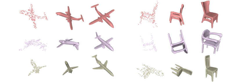
Figure 8. Reconstruction results of OccNet [Mescheder et al., 2019] via shape-pose disentanglement. An input point cloud on the left is disentangled to shape encoding and pose. OccNet decodes only the shape encoding yielding a canonical shape on the right column. The reconstruction is then transformed by the estimated pose as seen in the middle column. Meshes are extracted via Multiresolution IsoSurface Extraction (MISE) [Mescheder et al., 2019]

4.4. Reconstruction quality

We show qualitatively our point cloud reconstruction in Fig. 7. Please note that our goal is not to build a SOTA auto-encoder in terms of reconstruction, rather we learn to disentangle pose from shape via auto-encoding. Nonetheless, our auto-encoder does result in a pleasing result as shown in Fig. 7. Moreover, since we utilize AtlasNetV2[Deprelle et al., 2019] which utilizes a multiple patch-based decoder, we can examine which point belongs to which decoder. As our shape-encoding is both invariant to pose and consistent across different shapes, much like in the aligned scenario, each decoder assume some-what of semantic meaning, capturing for example the right wing of the airplanes. Please note that we do not enforce any structuring on the decoders.

4.5. 3D implicit reconstruction

We show that our encoder can be attached to a different reconstruction task by repeating OccNet [Mescheder et al., 2019] completion experiment. We replace OccNet encoder with our shape-pose disentagling encoder. The experiment is preformed with the same settings as in [Mescheder et al., 2019]. We use the subset of [Choy et al., 2016], and the point clouds are sub-sampled from the watertight mesh, containing only $300$ points and applied with a Gaussian noise. We have trained OccNet for $600K$ iterations and report the results of the best (reconstruction wise) checkpoint. We show in Fig. 8 a few examples of rotated point clouds (left), its implicit function reconstruction (middle) and the implicit function reconstruction in the canonical pose (right).

5. Conclusions

We have presented a stable and consistent canonical representation learning. To achieve a pose-invariant represenation, we have devised an $\mathbf{SE}(3)$-equivairant encoder, extending the VNN framework, to meet the requirements of canonical pose learning, i.e., learning rigid transformations. Our experiments show, both qualitatively and quantitatively, that our canonical representation is significantly more stable than recent approaches and has similar or better consistency, especially for diverse object classes. Moreover, we show that our approach is not limited to specific decoding mechanism, allowing for example to reconstruct canonical implicit neural field. In the future, we would like to explore the potential of our canonical representation for point cloud processing tasks requiring aligned settings, such as completion and unsupervised segmentation, where the canonical representation is learned on-the-fly, along with the task.

Appendix A $\mathbf{SE}(3)$-equivariance verification

In this section we verify that our VNT layers are indeed translation and rotation equivariant, as well as explicitly present other layers, not included in the paper.

A.1. Verifying $\mathbf{SE}(3)$-equivariant linear layer

We verify that the linear module $f_{\textrm{lin}}\left(\cdot;\mathbb{W}\right)$, defined via a weight matrix
$\mathbb{W}\in\mathcal{W}^{C^{\prime}\times C}$, acting on a vector-list feature $\mathbb{V}\in\mathbb{R}^{C\times 3}$, such that

(17) $$\mathcal{W}^{C^{\prime}\times C}=\left\{\mathbb{W}\in\mathbb{R}^{C^{\prime}\times C}\mid\textstyle{\sum_{j=1}^{C}}w_{i,j}=1\quad\forall i\in[1,C^{\prime}]\right\},$$

is $\mathbf{SE}(3)$-equivariant.

Let $\mathbb{w_{j}}\in\mathbb{R}^{C^{\prime}\times C}$ be the $j$ column of $\mathbb{W}$, and let $R\in\mathbb{R}^{3\times 3}$ be a rotation matrix and $T\in\mathbb{R}^{1\times 3}$ a translation vector. For $f_{\textrm{lin}}\left(\cdot;\mathbb{W}\right)$ to be $\mathbf{SE}(3)$-equivariant, the following must hold:

$$f_{\textrm{lin}}\left(\mathbb{V}R+\mathbbm{1}_{C}T\right)=\mathbb{W}\left(\mathbb{V}R+\mathbb{\mathbbm{1}}_{C}T\right)=\mathbb{W}\mathbb{V}R+\mathbb{W}\mathbb{\mathbbm{1}}_{C}T=$$

(18) $$=\mathbb{W}\mathbb{V}R+\left(\sum_{j=1}^{C}\mathbb{w}_{j}\right)T=(\mathbb{W}\mathbb{V})R+\mathbb{\mathbbm{1}}_{C^{\prime}}T,=f_{\textrm{lin}}(\mathbb{V})R+\mathbb{\mathbbm{1}}_{C^{\prime}}T,$$

where $\mathbbm{1}_{C}=[1,1,\dots,1]^{T}\in\mathbb{R}^{C\times 1}$ is a column vector of length $C$, and $\sum_{j=1}^{C}\mathbb{w_{j}}=\mathbbm{1}_{C^{\prime}}$, since $\left(\sum_{j=1}^{C}\mathbb{w_{j}}\right)[i]=\sum_{j=1}^{C}{w_{ij}}=1$ for $i=1,\dots,C^{\prime}$

A.2. Verifying $\mathbf{SE}(3)$-equivariant ReLU

We verify that the ReLU layer is $\mathbf{SE}(3)$-equivariant.

Let $\mathbb{V},\mathbb{V^{\prime}}\in\mathbb{R}^{C\times 3}$ be the input and output of a ReLU layer,

(19) $$\mathbb{V^{\prime}}=f_{\textrm{ReLU}}\left(\mathbb{V}\right).$$

Let ${\mathbb{v^{\prime}}\in\mathbb{R}^{1\times 3}}$ be a single vector, such that $\mathbb{v^{\prime}}\in\mathbb{V^{\prime}}$. As explained in Section 3.1 of the paper, we learn three translation equivariant linear maps, $\mathbb{Q},\mathbb{K},\mathbb{O}\in\mathcal{W}^{1\times C}$ projecting the input to $\mathbb{q},\mathbb{k},\mathbb{o}\in\mathbb{R}^{1\times 3}$, yielding an origin $\mathbb{o}$, a feature $\mathbb{q_{o}}=\mathbb{q}-\mathbb{o}$ and a direction $\mathbb{k_{o}}=\mathbb{k}-\mathbb{o}$. The ReLU layer for a single vector neuron is then defined via

(20) $$\mathbb{v^{\prime}}=\begin{cases}\mathbb{o}+\mathbb{q_{o}}&\text{if}\quad{\left\langle\mathbb{q_{o}},\mathbb{k_{o}}\right\rangle}\geq 0,\\ \mathbb{o}+\mathbb{q_{o}}-{\left\langle\mathbb{q_{o}},\frac{\mathbb{k_{o}}}{\left\lVert\mathbb{k_{o}}\right\rVert}\right\rangle}\frac{\mathbb{k_{o}}}{\left\lVert\mathbb{k_{o}}\right\rVert},&\text{otherwise}.\end{cases}.$$

$\mathbb{q},\mathbb{k},\mathbb{o}$ are $\mathbf{SE}(3)$-equivariant and according to Eq .(7) of the paper, $\mathbb{q_{o}},\mathbb{k_{o}}$ are translation invariant (and rotation equivariant) as they are the subtraction of two $\mathbf{SE}(3)$-equivariant vector neurons, thus, the condition term ${\left\langle\mathbb{q_{o}},\mathbb{k_{o}}\right\rangle}$ is also translation invariant. As shown in VNN [6], the inner product of two rotation equivariant vector-neurons is rotation invariance. Similarly here, assume the input $\mathbb{V}$ is rotated with a rotation matrix $R\in\mathbb{R}^{3\times 3}$, then

(21) $${\left\langle\mathbb{q_{o}}R,\mathbb{k_{o}}R\right\rangle}=\mathbb{q_{o}}RR^{T}\mathbb{k_{o}}=\mathbb{q_{o}}\mathbb{k_{o}}^{T}={\left\langle\mathbb{q_{o}},\mathbb{k_{o}}\right\rangle}$$

To conclude, the condition term ${\left\langle\mathbb{q_{o}},\mathbb{k_{o}}\right\rangle}$ is $\mathbf{SE}(3)$-invariant.

When ${\left\langle\mathbb{q_{o}},\mathbb{k_{o}}\right\rangle}\geq 0$, the output vector neuron $\mathbb{v^{\prime}}=\mathbb{o}+\mathbb{q_{o}}=\mathbb{q}$, and thus it is $\mathbf{SE}(3)$-equivariant.

When ${\left\langle\mathbb{q_{o}},\mathbb{k_{o}}\right\rangle}<0$ the output vector neuron is

(22) $$\mathbb{o}+\mathbb{q_{o}}-{\left\langle\mathbb{q_{o}},\frac{\mathbb{k_{o}}}{\left\lVert\mathbb{k_{o}}\right\rVert}\right\rangle}\frac{\mathbb{k_{o}}}{\left\lVert\mathbb{k_{o}}\right\rVert},$$

Similarly to Eq .(21) the term

(23) $${\left\langle\mathbb{q_{o}},\frac{\mathbb{k_{o}}}{\left\lVert\mathbb{k_{o}}\right\rVert}\right\rangle}\frac{1}{\left\lVert\mathbb{k_{o}}\right\rVert}=\frac{{\left\langle\mathbb{q_{o}},\mathbb{k_{o}}\right\rangle}}{{\left\langle\mathbb{k_{o}},\mathbb{k_{o}}\right\rangle}},$$

is also $\mathbf{SE}(3)$-invariant.

We can now easily prove that if the input $\mathbb{V}$ is rotated with a rotation matrix $R\in\mathbb{R}^{3\times 3}$ and translation vector $T\in\mathbb{R}^{1\times 3}$, then

$$\mathbb{v^{\prime}}= \mathbb{o}R+\mathbbm{1}_{C}T+\mathbb{q_{o}}R-{\left\langle\mathbb{q_{o}},\frac{\mathbb{k_{o}}}{\left\lVert\mathbb{k_{o}}\right\rVert}\right\rangle}\frac{\mathbb{k_{o}}R}{\left\lVert\mathbb{k_{o}}\right\rVert}$$

(24) $$=\left(\mathbb{o}+\mathbb{q_{o}}-{\left\langle\mathbb{q_{o}},\frac{\mathbb{k_{o}}}{\left\lVert\mathbb{k_{o}}\right\rVert}\right\rangle}\frac{\mathbb{k_{o}}}{\left\lVert\mathbb{k_{o}}\right\rVert}\right)R+\mathbbm{1}_{C}T=\mathbb{v^{\prime}}R+\mathbbm{1}_{C}T,$$

Thereby completing the proof.

A.3. VNT-LeakyReLU

LeakyReLU is defined in a similar manner to the ReLU layer, with slight modification to the output vector neuron, given by

(25) $$\mathbb{v^{\prime}}=\alpha\mathbb{q}+\left(1-\alpha\right)\mathbb{v^{\prime}}_{\textrm{ReLU}},$$

where $\alpha\in\mathbb{R}$

Easy to see that the $\mathbb{v^{\prime}}$ is $\mathbf{SE}(3)$-equivariant.

A.4. VNT-MaxPool

Given a set of vector-neuron list $\mathcal{V}\in\mathbb{R}^{N\times C\times 3}$, we learn two linear maps $\mathbb{K},\mathbb{O}\in\mathcal{W}^{C\times C}$, shared between $\mathbb{V_{n}}\in\mathcal{V}$.

We obtain a translation invariant direction

(26) $$\mathcal{K}=\left\{\mathbb{K}\mathbb{V_{n}}-\mathbb{O}\mathbb{V_{n}},\right\}_{n=1}^{N}$$

and a translation invariant features

(27) $$\mathcal{Q}=\left\{\mathbb{V_{n}}-\mathbb{O}\mathbb{V_{n}}\right\}_{n=1}^{N}.$$

The VNT-MaxPool is defined by

(28) $$f_{MAX}\left(\mathcal{V}\right)[c]=\mathbb{V}_{n^{*}}[c]$$

(29) $$\textrm{where}\quad n^{*}=\underset{n}{\operatorname*{arg\,max}}{\left\langle\mathbb{Q_{n}}[c],\mathbb{K_{n}}[c]\right\rangle},$$

where $\mathbb{Q_{n}}\in\mathcal{Q}$ and $\mathbb{K_{n}}\in\mathcal{K}$. Since $\mathbb{Q_{n}}$, $\mathbb{K_{n}}$ are translation invariant, and their inner product is also rotation invariant the selection process of $n^{*}$ for every channel $c$ is invariant to $\mathbf{SE}(3)$. We note that both $\mathbb{K},\mathbb{O}$ can be shared across vector-neurons.

Appendix B Implementations Details

B.1. Encoder architecture

In this section we elaborate on our encoder architecture. Our encoder contains VNT layers following with VNN layers as reported in Table 2. LinearLeakyReLU stands for the leakyReLU with feature learning $\mathcal{Q}$. For the exact VNN layers definition (and specifically STNkd) we refer the reader to VNN [6].

Table 2. Our shape-pose disentangling encoder architecture.

Name	Input channel	Output channel	Type
LinearLeakyReLU	$3$	$64$//$3$	VNT
LinearLeakyReLU	$64$//$3$	64//3	VNT
T-invariant	$64$//$3$	$64$//$3$	VNT
LinearLeakyReLU	$64$//$3$	$64$//$3$	VNN
STNkd+concat	$64$//$3$	$2\cdot$($64$//$3$)	VNN
LinearLeakyReLU	$2\cdot$($64$//$3$)	$2\cdot$($64$//$3$)	VNN
LinearLeakyReLU	$2\cdot$($64$//$3$)	$170$	VNN
BatchNorm	$170$	$170$	VNN
Meanpool+concat	$170$	$340$	VNN
R-invariant	$340$	$340$	VNN
Flatten	$340\cdot 3$	$1020$	Regular
Max-pool	$1020$	$1020$	Regular

Appendix C Implicit reconstruction

Occupancy network reconstruction from a point clouds $X\in\mathbb{R}^{N\times 3}$, with a learned embedding $\mathbb{z}\in\mathcal{X}$ , learns a mapping function $f_{\theta}(p,\mathbb{z}):\mathbb{R}^{3}\times\mathcal{X}\rightarrow[0,1]$. In occupancy network completion experiment, the point cloud is sampled from the watertight mesh, and the mesh is used as supervision to sample $M$ training point $\left\{p_{i}\right\}_{i=1}^{M}$ inside and outside the mesh, indicated by $\left\{o_{i}\right\}\in[0,1]^{M}$. We follow the same experiment, with slight changes. We feed our learned pose-invariant encoding $\mathbb{Z_{s}}$ through $f_{\theta}$, and project the points $\left\{p_{i}\right\}$ from the input pose to the learned canonical pose by:

(30) $$\tilde{p}_{i}=(p_{i}-\tilde{T})\tilde{R}^{T}\quad i=1,\dots,M$$

Therefore, our reconstruction loss is

(31) $$\mathcal{L}_{\textit{rec}}=\sum_{i=1}^{M}{\mathcal{L}_{\textrm{BCE}}\left(f_{\theta}(\tilde{p}_{i},\mathbb{Z_{s}}),o_{i}\right)},$$

where $\mathcal{L}_{\textrm{BCE}}$ is binary cross entropy loss. For implicit reconstruction we have found it beneficial to train the network in an alternating approach, where at the first phase we backward w.r.t $\mathcal{L}_{\textit{rec}}$ and in the second phase we backward w.r.t

(32) $$\mathcal{L}_{2}=\lambda_{1}\mathcal{L}_{\textit{ortho}}+\lambda_{2}\mathcal{L}^{\textit{aug}}_{\textit{consist}}.$$

Appendix D Additional results

D.1. Augmentations ablation

In this section we specify in more details our augmentations, which can be seen in Fig. 9, and ablate their individual donation to the consistency of our canonical representation. Our augmentations are Furthest point sampling (FPS), with random number of points $N_{\textrm{FPS}}=\textrm{U}\left(300,500\right)$ per batch, K-NN removal (KNN), where a point is randomly selected on the point cloud, and its $N_{\textrm{KNN}}=100$ points are removed, Gaussian Noise added to the point clouds with $\mu=0$ and $\sigma=0.025$, a re-sampling augmentations (Resample) where we re-select which $N=1024$ to sample from the original point cloud, and canonical rotation (Can), where the point cloud reconstruction in its canonical representation is rotated and transformed to create a supervised version of itself. Since our method is pose-invariant by construction, different augmentations have no effect on the stability, thus, we ablate only w.r.t the consistency as reported in Table 3. We ablate the donation of each augmentation by removing it from the training process and measuring the consistency as defined in the paper. Evidently, the lesser factor is the noise addition augmentation, while KNN and FPS donate the most to the consistency metric.

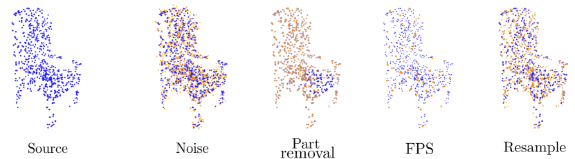
Figure 9. Point cloud augmentations. The source point cloud on the left (blue), is modified (brown) to supervise a rotation and translation learning invariant of the shape.

Table 3. Consistency of different augmentations composition (lower is better). Each column but the last represents the absence of an augmentation, indicating its importance to the consistency metric.

	-FPS	- Noise	-KNN	-Resample	-Can	All
Airplanes	52.31	50.0	$66.4$	$50.5$	$53.7$	${\bf 49.9}$
Chairs	27.31	24.41	$27.31$	$25.3$	$25.1$	$\mathbb{24.31}$

D.2. Pose consistency

We present more canonical alignment results for point clouds and implicit function reconstruction Fig. 10, Fig. 11, Fig. 12 and Fig. 13.

In addition, we experiment with partial dataset for shape completion derived from ShapeNet (See Yuan et al. ”Pcn: Point completion network”). The partial points clouds are a projection of 2.5D depth maps of the model into 3D point clouds. The dataset contains $8$ such partial point clouds per model. As can be seen in Fig. 14 while learning a consistent canonical pose is difficult for partial shapes, our canonical pose is reasonable and mostly consistent. Although, misalignment is apparent in the consistency histogram, please note that no complete point cloud is present in this setting, and no hyper-parameter tuning was done.

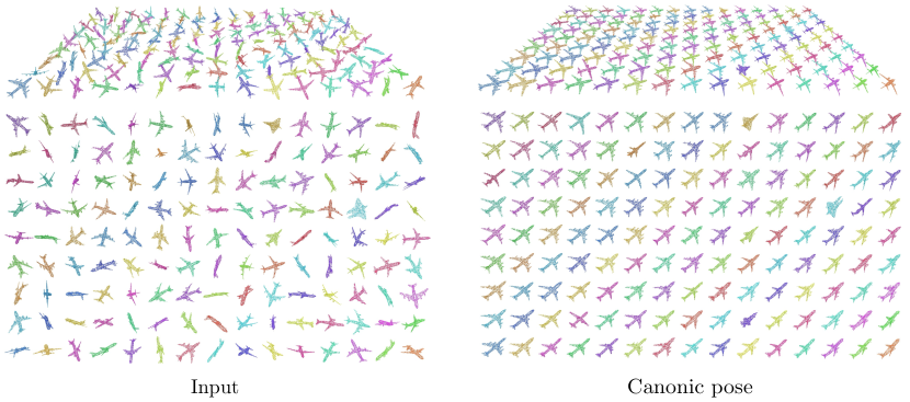
Figure 10. More results of planes in canonic representations. The planes on the left are randomly translated and rotated, as seen from a side view (first row) and top view (second row). Our canonical representation, on the right, exhibit good alignment across different instances both in orientation and position.

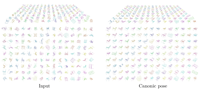
Figure 11. More results of chairs in canonic representations. The chairs on the left are randomly translated and rotated, as seen from a side view (first row) and top view (second row). Our canonical representation, on the right, exhibit good alignment across different instances both in orientation and position.

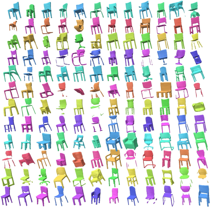
Figure 12. More results of implicit function reconstruction for chairs in canonic representations. Our canonical representation exhibit good alignment across different instances both in orientation and position.

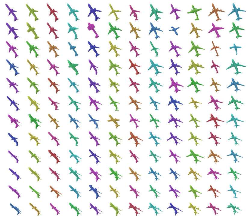
Figure 13. More results of implicit function reconstruction for planes in canonic representations. Our canonical representation exhibit good alignment across different instances both in orientation and position.

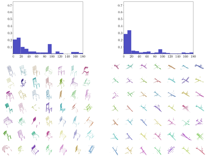
Figure 14. Consistency of the canonical pose for partial shapes of planes and chairs. While our method is not directly optimized to achieve canonic alignment of partial shapes due to occlusions, it has reasonable performances has can be seen in the histogram of the first row and from samples in the second row.

D.3. Stability

Please see the attached videos for stability visualization, divided to two sub-folders for chairs and airplanes. In each video, we sample a single point cloud and rotate it with multiple random rotation matrices. We feed the rotated point cloud (see on the left of each video) through Compass, Canonical Capsules and Our method, and show the input point cloud in canonical pose for all methods. Our method reconstruct a $\mathbf{SE}(3)$-invariant canonical representation and a $\mathbf{SE}(3)$-equivariant pose estimation, thus, almost no changes are observable in the canonical representation, while both Canonical Capsules and Compass exhibit instability in the canonical pose estimation.

References

- [1]
- Bar-Itzhack [1975] Itzhack Y Bar-Itzhack. 1975. Iterative optimal orthogonalization of the strapdown matrix. IEEE Trans. Aerospace Electron. Systems 1 (1975), 30–37.
- Chang et al. [2015] Angel X Chang, Thomas Funkhouser, Leonidas Guibas, Pat Hanrahan, Qixing Huang, Zimo Li, Silvio Savarese, Manolis Savva, Shuran Song, Hao Su, et al. 2015. Shapenet: An information-rich 3d model repository. arXiv preprint arXiv:1512.03012 (2015).
- Choy et al. [2016] Christopher B Choy, Danfei Xu, JunYoung Gwak, Kevin Chen, and Silvio Savarese. 2016. 3d-r2n2: A unified approach for single and multi-view 3d object reconstruction. In European conference on computer vision. Springer, 628–644.
- Cohen et al. [2018] Taco S Cohen, Mario Geiger, Jonas Köhler, and Max Welling. 2018. Spherical cnns. arXiv preprint arXiv:1801.10130 (2018).
- Cohen and Welling [2016] Taco S Cohen and Max Welling. 2016. Steerable cnns. arXiv preprint arXiv:1612.08498 (2016).
- Deng et al. [2021] Congyue Deng, Or Litany, Yueqi Duan, Adrien Poulenard, Andrea Tagliasacchi, and Leonidas J Guibas. 2021. Vector neurons: A general framework for SO (3)-equivariant networks. In Proceedings of the IEEE/CVF International Conference on Computer Vision. 12200–12209.
- Deprelle et al. [2019] Theo Deprelle, Thibault Groueix, Matthew Fisher, Vladimir Kim, Bryan Russell, and Mathieu Aubry. 2019. Learning elementary structures for 3D shape generation and matching. In Advances in Neural Information Processing Systems. 7433–7443.
- Esteves et al. [2018] Carlos Esteves, Christine Allen-Blanchette, Ameesh Makadia, and Kostas Daniilidis. 2018. Learning so (3) equivariant representations with spherical cnns. In Proceedings of the European Conference on Computer Vision (ECCV). 52–68.
- Groueix et al. [2018] Thibault Groueix, Matthew Fisher, Vladimir G Kim, Bryan C Russell, and Mathieu Aubry. 2018. A papier-mâché approach to learning 3d surface generation. In Proceedings of the IEEE conference on computer vision and pattern recognition. 216–224.
- Gu et al. [2020] Jiayuan Gu, Wei-Chiu Ma, Sivabalan Manivasagam, Wenyuan Zeng, Zihao Wang, Yuwen Xiong, Hao Su, and Raquel Urtasun. 2020. Weakly-supervised 3D shape completion in the wild. In European Conference on Computer Vision. Springer, 283–299.
- Hamdi et al. [2021] Abdullah Hamdi, Silvio Giancola, and Bernard Ghanem. 2021. Mvtn: Multi-view transformation network for 3d shape recognition. In Proceedings of the IEEE/CVF International Conference on Computer Vision. 1–11.
- Liu et al. [2020] Zhe Liu, Xin Zhao, Tengteng Huang, Ruolan Hu, Yu Zhou, and Xiang Bai. 2020. Tanet: Robust 3d object detection from point clouds with triple attention. In Proceedings of the AAAI Conference on Artificial Intelligence, Vol. 34. 11677–11684.
- Ma et al. [2022] Xu Ma, Can Qin, Haoxuan You, Haoxi Ran, and Yun Fu. 2022. Rethinking Network Design and Local Geometry in Point Cloud: A Simple Residual MLP Framework. In International Conference on Learning Representations.
- Mescheder et al. [2019] Lars Mescheder, Michael Oechsle, Michael Niemeyer, Sebastian Nowozin, and Andreas Geiger. 2019. Occupancy networks: Learning 3d reconstruction in function space. In Proceedings of the IEEE/CVF Conference on Computer Vision and Pattern Recognition. 4460–4470.
- Novotny et al. [2019] David Novotny, Nikhila Ravi, Benjamin Graham, Natalia Neverova, and Andrea Vedaldi. 2019. C3dpo: Canonical 3d pose networks for non-rigid structure from motion. In Proceedings of the IEEE/CVF International Conference on Computer Vision. 7688–7697.
- Park et al. [2019] Jeong Joon Park, Peter Florence, Julian Straub, Richard Newcombe, and Steven Lovegrove. 2019. Deepsdf: Learning continuous signed distance functions for shape representation. In Proceedings of the IEEE/CVF Conference on Computer Vision and Pattern Recognition. 165–174.
- Qi et al. [2017a] Charles R Qi, Hao Su, Kaichun Mo, and Leonidas J Guibas. 2017a. Pointnet: Deep learning on point sets for 3d classification and segmentation. In Proceedings of the IEEE conference on computer vision and pattern recognition. 652–660.
- Qi et al. [2017b] Charles Ruizhongtai Qi, Li Yi, Hao Su, and Leonidas J Guibas. 2017b. Pointnet++: Deep hierarchical feature learning on point sets in a metric space. Advances in neural information processing systems 30 (2017).
- Rempe et al. [2020] Davis Rempe, Tolga Birdal, Yongheng Zhao, Zan Gojcic, Srinath Sridhar, and Leonidas J Guibas. 2020. Caspr: Learning canonical spatiotemporal point cloud representations. Advances in neural information processing systems 33 (2020), 13688–13701.
- Shi et al. [2019] Shaoshuai Shi, Xiaogang Wang, and Hongsheng Li. 2019. Pointrcnn: 3d object proposal generation and detection from point cloud. In Proceedings of the IEEE/CVF conference on computer vision and pattern recognition. 770–779.
- Spezialetti et al. [2020] Riccardo Spezialetti, Federico Stella, Marlon Marcon, Luciano Silva, Samuele Salti, and Luigi Di Stefano. 2020. Learning to orient surfaces by self-supervised spherical cnns. arXiv preprint arXiv:2011.03298 (2020).
- Sun et al. [2021] Weiwei Sun, Andrea Tagliasacchi, Boyang Deng, Sara Sabour, Soroosh Yazdani, Geoffrey E Hinton, and Kwang Moo Yi. 2021. Canonical Capsules: Self-Supervised Capsules in Canonical Pose. Advances in Neural Information Processing Systems 34 (2021).
- Thomas et al. [2018] Nathaniel Thomas, Tess Smidt, Steven Kearnes, Lusann Yang, Li Li, Kai Kohlhoff, and Patrick Riley. 2018. Tensor field networks: Rotation-and translation-equivariant neural networks for 3d point clouds. arXiv preprint arXiv:1802.08219 (2018).
- Wang et al. [2019] Yue Wang, Yongbin Sun, Ziwei Liu, Sanjay E Sarma, Michael M Bronstein, and Justin M Solomon. 2019. Dynamic graph cnn for learning on point clouds. Acm Transactions On Graphics (tog) 38, 5 (2019), 1–12.
- Weiler et al. [2018] Maurice Weiler, Mario Geiger, Max Welling, Wouter Boomsma, and Taco Cohen. 2018. 3d steerable cnns: Learning rotationally equivariant features in volumetric data. arXiv preprint arXiv:1807.02547 (2018).
- Xu et al. [2019] Qiangeng Xu, Weiyue Wang, Duygu Ceylan, Radomir Mech, and Ulrich Neumann. 2019. Disn: Deep implicit surface network for high-quality single-view 3d reconstruction. Advances in Neural Information Processing Systems 32 (2019).
- Yang et al. [2018] Yaoqing Yang, Chen Feng, Yiru Shen, and Dong Tian. 2018. Foldingnet: Point cloud auto-encoder via deep grid deformation. In Proceedings of the IEEE conference on computer vision and pattern recognition. 206–215.
- Yang et al. [2020] Zetong Yang, Yanan Sun, Shu Liu, and Jiaya Jia. 2020. 3dssd: Point-based 3d single stage object detector. In Proceedings of the IEEE/CVF conference on computer vision and pattern recognition. 11040–11048.