Multiple Charged Meson Production in Exclusive $B_{c}$ Decays: $K+4\pi,$$KK+3\pi$, $7\pi$ Cases.

Abstract

Theoretical analysis of three exclusive decays, $B_{c}\to\psi^{(^{\prime})}+\mathcal{R},$where $R=K+4\pi,$$KK+3\pi$, or $7\pi$, is given. Using the factorization method and the resonance approximation (methods proved to be very useful in the analysis of some other similar decays), we have obtained analytical expressions of the required amplitudes and created distributions over some interesting mass combinations. Presented results could be used for comparison with forthcoming experimental data and better understanding of the nature of heavy quarkonia.

I Introduction

Heavy quarkonia mesons, that is particles that in valence approximation are built from heavy (i.e. $c$ of $b$) pairs can be considered as a unique laboratory to study strong interaction both in perturbative and non-perturbative regimes. On the partonic level the processes of their production and decay can be described in terms of creation or annihilation of the heavy quark, that hadronizes later into experimentally obesrved particle. Doubly heavy meson with an opened flavor,$B_{c}=bc$ take an intermediate position between charmonium $\left(c\bar{c}\right)$ and bottomonium $\left(b\bar{b}\right)$ particles, that allows one to use it as a test for models that were developed to describe heacy quarkonium particles with hidden flavor. Nice theoretical review concerning different properties of this particle can be found, for example, in paper Gershtein et al. (1995)

The presented paper is devoted to phenomenological analysis of some exclusive $B_{c}$-meson decay with the vector charmonium production accomplished by $K+4\pi$, $KK+3\pi$ or $7\pi$. This work is a continuation of series of papers at were devoted to production of other systems of light mesons in the similar processes.

General idea used in all these works is simple. It is well known that in valence approximation $B_{c}$-meson is built from $b$- and $c$-quarks. Exclusive decay of this particle into vector charmonium and some set of light mesons on the partonic level can be described by the weak decay of the constituent $b$-quark: $b\to Wc$. Produced $W$ boson hadronizes into the final system of light particles, while $c$-quark with a spectator $\bar{c}$ forms $J/\psi$ or $\psi(2S)$ . The subprocess $B_{c}\to W\psi^{(^{\prime})}$ can be described in terms of weak $B_{c}$-meson form-factors. The suitable theoretical model for the W- boson hadronization, on the other hand, is the so-called resonance approach.

Described above simple model turned out to be surprisingly powerful. It was used to describe decays $B_{c}\to J/\psi+3\pi$, etc., and the predictions for differential distributions and integrated branching fractions are in good agreement withe experimental results. In the present paper we are extending the analysis to three new decays.

The rest of the paper is organized as follows. In the next section a short description of the adopted approach is given and the parametrization of the $B_{c}$-meson’s form-factors is resented. Section 3 is devoted to theoretical description of same observed already decays, that mile be used as subprocesses for new ones. These new decays will be studied in section 4, while the last section is reserved to some discussion and conclusion.

II Exclusive $B_{c}$ decays

In the partonic approximation $B_{c}$ meson is build from $b\bar{c}$ quarks, so its exclusive decays into vector charmonium and a set of light mesons can be described as a weak decay of the constituent $b$ quark. Produced $c$ with a spectator $\bar{c}$ forms the final charmonium, while $W$-boson hadronizes into the final system of light mesons $\mathcal{R}$. The schematic Feynman diagram of this process is shown in figure 1.

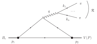
Figure 1: Feynman diagram for $B_{c}\to\psi\mathcal{R}$ decay

In the factorization approximation this diagram can be written in the form

$$\mathcal{M} = \frac{G_{F}V_{bc}}{\sqrt{2}}a_{1}H^{\mu}\epsilon_{\mu}^{(\mathcal{R})},$$

where the Wilson coefficient $a_{1}(m_{b})\approx 1.14$ describes the effect of final state interaction Buchalla et al. (1996), $G_{F}$ is a Fermi coupling constant, $V_{bc}$ is a corresponding coefficient of the CKM matrix, while $H^{\mu}$ and $\epsilon_{\mu}^{(\mathcal{R})}$ are the amplitudes of the $B_{c}\to\psi W$ and $W\to R$ transitions respectively.

Let us define the the first amplitude first. It is clear, that it can depend only on the momenta of the initial and final heavy mesons $p_{1,2}$. There are several ways how it can be written in the Lorentz-invariant form and in our paper we will use the parametrization adopted, for example, in paper Kiselev et al. (2000a):

$$H_{\mu} = \left[2M_{\psi}A_{0}\left(q^{2}\right)\frac{q^{\mu}q^{\nu}}{q^{2}}+\left(M_{B_{c}}-M_{\psi}\right)A_{1}\left(q^{2}\right)\left(g^{\mu\nu}-\frac{q^{\mu}q^{\nu}}{q^{2}}\right)-\right.$$

$$\left.A_{2}\left(q^{2}\right)\left(p_{1}^{\mu}+p_{2}^{\mu}-\frac{M_{B_{c}}^{2}-M_{\psi}^{2}}{q^{2}}q^{\mu}\right)-\frac{2iV\left(q^{2}\right)}{M_{B_{c}+M_{\psi}}}e^{\mu\nu\alpha}p_{1\alpha}p_{2}\right]\epsilon_{\nu}^{(\psi)}.$$

Here $\epsilon^{(\psi)}$ is the polarization vector of final charmonium meson and $A_{0,1,2}\left(q^{2}\right)$, $V\left(q^{2}\right)$ are axial and vector form factors of $B_{c}\to\psi W$ transition. It is clear that these functions cannot be determined from perturbative theory, so some other approach should be used, such as for example QCD sum rules Huang and Zuo (2007); Kiselev et al. (2000b, c, a); Kiselev (2002), different potential quark models Kiselev et al. (1993); Gershtein et al. (1995, 1997); Colangelo and De Fazio (2000); Ivanov et al. (2005), light-front models Anisimov et al. (1999); Choi and Ji (2009a, b), etc. In our paper we will use form-factors sets presented in paper Kiselev et al. (2000a).

These form factors can be parametrized as

$$F\left(q^{2}\right) = \frac{F\left(0\right)}{1-q^{2}/m_{fit}^{2}},$$

where $q^{2}=\left(p_{1}-p_{2}\right)^{2}$ is the transferred momentum squared and the values of function at zero and maximal agruments are listed in table 1.

	$F(0)$	$F\left(q_{max}^{2}=M_{B_{c}}^{2}-M_{J/\psi}^{2}\right)$		$F(0)$	$F\left(q_{max}^{2}=M_{B_{c}}^{2}-M_{J/\psi}^{2}\right)$
$A_{0}$	0.60	1.6	$A_{2}$	0.69	1.4
$A_{1}$	0.63	1.3	$V$	1.0	2.1

Table 1: Parameters of the $B_{c}\to\psi^{(^{\prime})}W$ transition form factors

All information about the final system $\mathcal{R}$ is hidden in the effective polarization vector $\epsilon^{(\mathcal{R})}$. Its explicit form and numerical values depend on the number of final particles, their types and momenta. The only general issue is that in the limit of isospin conservation the relation $q^{\mu}\epsilon_{\mu}^{(\mathcal{R})}$ should hold, to the contribution of $A_{0}$ form factor vanishes. More detailed investigation requires some model assumptions on the physics of the underlying processes. Our previous works it was shown, that the resonance model gives the results that are in a good agreement with the experiment. In the framework of this model the amplitude of the process under consideration is written in the terms of hadronic resonances with suitable quantum numbers and the form of the amplitudes is chosen accordingly. In the present paper we will continue to use such an approach to describe the production of $\mathcal{R}=K+4\pi,$ $KK+3\pi$, and $7\pi$ states. It turns out that the corresponding processes can be explained in terms of previously considered and tested on experiment reactions with $KK\pi$, $3\pi$, $5\pi$ production. For this reason we will first consider these processes.

III Known Decays

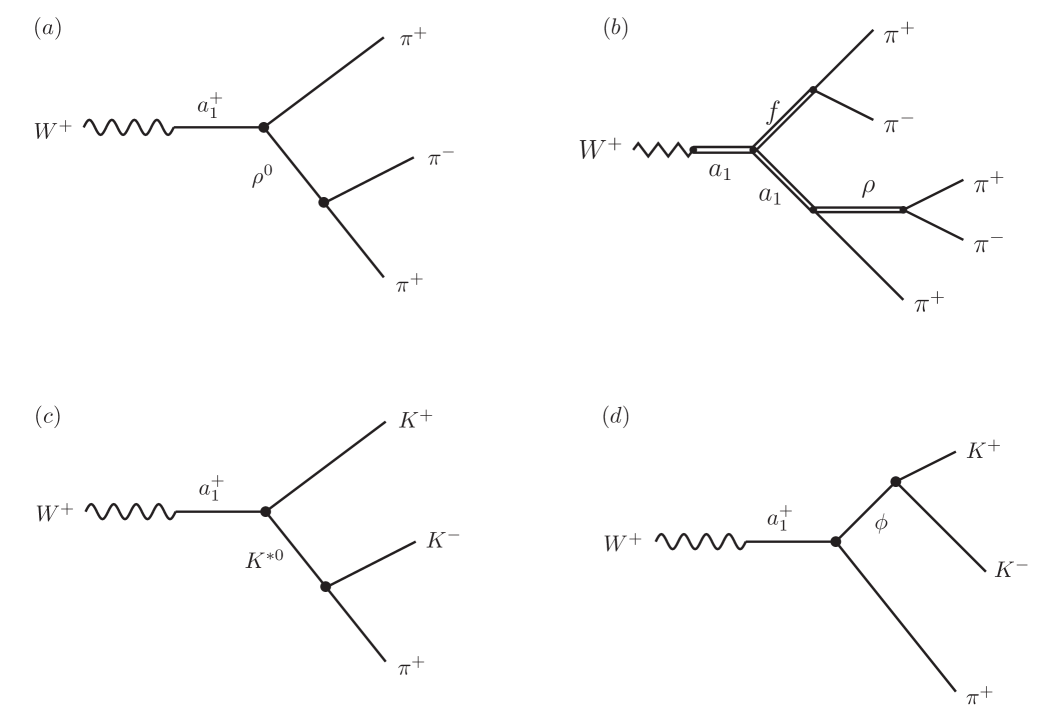
Figure 2: Feynman diagrams for old decay processes

Let us first consider $B_{c}\to\psi+3\pi$ decay. In resonance approximation it can be described by the diagram shown on figure 2(a). The corresponding amplitude can be written in the form

$$\epsilon_{(3\pi)}^{\mu}\left(Q\to k_{1}k_{2}k_{3}\right) \sim BW_{a1}\left(Q^{2}\right)\left(g_{\mu\alpha}-\frac{Q_{\mu}Q_{\alpha}}{Q^{2}}\right)q_{[13]}^{\alpha}BW_{\rho}\left(q_{\{13\}}^{2}\right)+\left\{q_{1}\Leftrightarrow q_{2}\right\},$$

where $q_{1,2,3}$ are the momenta of two final $\pi^{+}$ mesons and $\pi^{-}$ meson, $Q=q_{1}+q_{2}+q_{3}$ is the total momentum of virtual $a_{1}$, and notations

$$q_{[ij]}^{\alpha} = q_{i}^{\alpha}-q_{j}^{\alpha},\qquad q_{\{ij\}}^{\alpha}=q_{i}^{\alpha}+q_{j}^{\alpha}$$

were introduced. As you can see, we are using usual Feynman rules to write this relation and general from of the vertices is determined by quantum numbers of the participating particles. For example, the interaction $(q_{1}-q_{3})_{\alpha}$ was selected for $\rho\to\pi\pi$ decay since we are dealing with vector particle decay into two scalars, so P-wave is in place. The only interesting thing in the above equation is the propagators of the virtual $a_{1}$ and $\rho$ mesons. Following Flatte (1976) they are written using Flatte parametrization, where the energy dependence of the resonance width is taken into account:

$$BW_{a}\left(q^{2}\right) = \frac{M_{a}^{2}}{M_{a}^{2}-q^{2}-iM_{a}\Gamma_{a}(q)},$$

$$BW_{\rho}\left(q^{2}\right) = \frac{1}{1+\beta}\left[\frac{M_{\rho}^{2}}{M_{\rho}^{2}-q^{2}-iM_{\rho}\Gamma_{\rho}\left(q^{2}\right)}+\beta\frac{M_{\rho^{\prime}}^{2}}{M_{\rho^{\prime}}^{2}-q^{2}-iM_{\rho^{\prime}}\Gamma_{\rho^{\prime}}\left(q^{2}\right)}\right]$$

This process was studied theoretically in works Berezhnoy et al. (2011); Luchinsky (2012); Kuhn and Was (2008)and later experimental confirmation by the LHCb collaboration followed Aaij et al. (2012) As you can see from figure 3(a), the agreement between theory and experiment is pretty good.

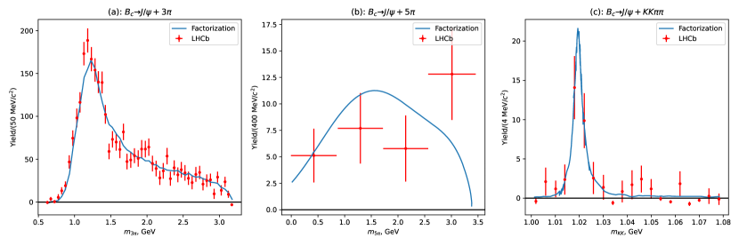
Figure 3: Comparison of theoretical predictions (blue line) with experiment (red dots).LHCb results shown in the left, center and right figures were published in papers Aaij et al. (2022), Aaij et al. (2014) and Aaij et al. (2022) respectively.

This process can be used as a building block to describe the production of the higher number of charged $\pi$ mesons, the corresponding Feynman diagram is shown in figure 2(b). The amplitude of this diagram is equal to

$$\epsilon_{(5\pi)}^{\mu} = BW_{a}\left(Q^{2}\right)BW_{f}\left(\left(q_{4}+q_{5}\right)^{2}\right)\epsilon_{(3\pi)}^{\mu}\left(q_{1},q_{2},q_{3}\right)+\text{symmetrization},$$

and the comparison of theoretical Luchinsky (2012) and experimental Aaij et al. (2017) distributions in shown in figure 3(b). As you can see, the agreement is again quite reasonable.

Let is consider now production of $KK\pi$ state. Two Feynman diagrams, that were used to describe it, are shown in figure 2(c), (d). The corresponding amplitude can be written in the following form

$$\epsilon_{KK\pi}^{\mu} = BW_{a}\left(Q^{2}\right)BW_{K^{*}}\left(q_{\{12\}}^{2}\right)q_{[12]}^{\mu}$$

Figure 3(c) shows that there is a good agreement between theoretical Luchinsky (2013) and experimental Aaij et al. (2022) results.

IV New Decays

In this section three new decays will be described, we will present amplitudes of these processes and theoretical predictions for some typical distributions.

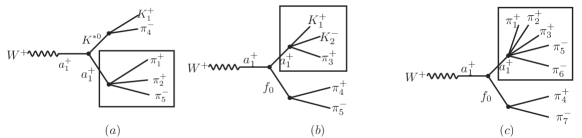
Figure 4: Diagram for $W\to\mathcal{R}$ transition

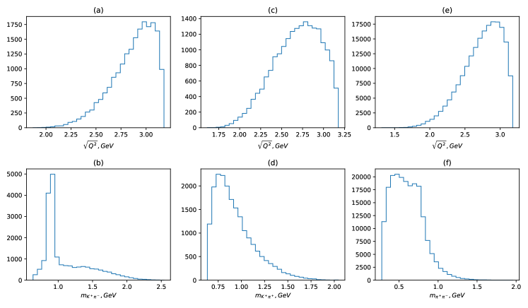
Figure 5: Distributions in $B_{c}\to J/\psi+\mathcal{R}$ decays:

Let us consider $\mathcal{R}=K^{+}\pi^{+}\pi^{+}\pi^{-}\pi^{-}$ final state first. In the resonance approximation $W$-boson hadronization into this system of light particles can be described by the diagram shown in figure 4(a). As you can see, this diagram includes $a_{1}\to 3\pi$ transition as a subprocess, so we can use presented above parametrization to describe it. The form of the other vertices’ amplitudes is easily determined by the quantum numbers of the interacting particles. As a result, the following form of the transition amplitude was used later:

$$\epsilon_{K4\pi}^{\mu} = BW_{a}\left(Q^{2}\right)BW_{K^{*}}\left(q_{\{14\}}^{2}\right)e^{\mu\nu\alpha\beta}q_{[14]}^{\nu}\left(q_{\{14\}}-q_{\{234\}}\right)^{\alpha}\epsilon_{(3\pi)}^{\beta}\left(q_{2,}q_{3,}q_{5}\right).$$

In figure 5(a), (b) some distributions are shown. On the last figure in the $m_{K\pi}$ system you can clearly see a peak caused by $K^{*0}$ resonance.

The subprocess $a_{1}\to KK\pi$, on the other hand, can be used in production of $KK+3\pi$ final state. The diagram is shown in figure 4(b) and the corresponding can be written in the form

$$\epsilon_{KK3\pi}^{\mu} = BW_{a}\left(Q^{2}\right)BW_{f}\left(q_{\{45\}}^{2}\right)\epsilon_{KK\pi}^{\mu}\left(q_{1}q_{2}q_{3}\right)+\text{symmetrization}.$$

In figure 5(c), (d) some distributions of the corresponding hadronic process are shown. Note that in this case there are no peaks in the $m_{K\pi}$ spectrum since there are no resonances in $K^{+}\pi^{+}$ channel.

The final process to be considered in our article is $B_{c}\to\psi^{(^{\prime})}+7\pi$ decay. The corresponding $W$-boson hadronization diagram is shown in figure 4(c).. As you can see, this reaction includes $a_{1}\to 5\pi$ transition as a subprocess, to its amplitude is written as

$$\epsilon_{7\pi}^{\mu} = BW_{a}\left(Q^{2}\right)BW_{f}\left(q_{\{47\}}^{2}\right)\epsilon_{5\pi}^{\mu}\left(q_{1,}q_{2},q_{3},q_{5},q_{6}\right)+\text{symmetrization}.$$

In figure 5(e), (f) distributions over the transferred momentum and mass of the $\pi^{+}\pi^{-}$ pair are shown. In the latter distribution you can see a small $\rho$-meson peak, which is almost hidden by the broad $f_{0}$ resonance.

V Conclusion

The presented paper is devoted to theoretical analysis of some exclusive $B_{c}$-meson decays. This work is a continuation of a series of papers, that are using the same approach for description of some other decays.

The theoretical model used in all these works is pretty simple. The reactions under consideration are represented as two-step process. The first step is weak $B_{c}$-meson decay into final victor charmonium and virtual $W$-boson, which then hadronizes into a system of light mesons. The first stage was described in terms of $B_{c}$-meson form-factors, while for the second stage the resonance approximation was used.

This simple method turned out to be surprisingly useful and able to produce theoretical predictions for a number of Bc-meson decays, that are in good agreement with experimental results. In the presented paper it was used to obtain analytical expressions for the amplitudes of three more decays: $B_{c}\to J/\psi+K+4\pi$, $B_{c}\to J/\psi+KK+3\pi$, and $B_{c}\to J/\psi+7\pi$. In addition, the numerical analysis of these reactions was performed and same interesting differential distributions can be found in thins work.

There is, of course, lot of work to be done in this field. For example, there are same unknown normalization constants in the used model, that cannot be determined from experimental data. For this reason we do not make predictions for the branching fractions of the considered decays, only normalized distributions are presented. Calculation of the branching fractions will be the topic of our future work.

The author would like to thank Dr. A. Likhoded, Dr. I. Belyaev, and Dr. D. Pereima for useful, stimulating, and motivating discussions. This research was done with support of RFBR grant 20-02-00154 A.

References

- Gershtein et al. (1995) S. S. Gershtein, V. V. Kiselev, A. K. Likhoded, and A. V. Tkabladze, Phys. Usp. 38, 1 (1995), eprint hep-ph/9504319.
- Buchalla et al. (1996) G. Buchalla, A. J. Buras, and M. E. Lautenbacher, Rev. Mod. Phys. 68, 1125 (1996), eprint hep-ph/9512380.
- Kiselev et al. (2000a) V. V. Kiselev, A. E. Kovalsky, and A. K. Likhoded, Nucl. Phys. B 585, 353 (2000a), eprint hep-ph/0002127.
- Huang and Zuo (2007) T. Huang and F. Zuo, Eur. Phys. J. C 51, 833 (2007), eprint hep-ph/0702147.
- Kiselev et al. (2000b) V. Kiselev, A. Likhoded, and A. Onishchenko, Nucl.Phys. B569, 473 (2000b), eprint hep-ph/9905359.
- Kiselev et al. (2000c) V. V. Kiselev, A. E. Kovalsky, and A. K. Likhoded, in 5th International Workshop on Heavy Quark Physics (2000c), eprint hep-ph/0006104.
- Kiselev (2002) V. V. Kiselev (2002), eprint hep-ph/0211021.
- Kiselev et al. (1993) V. V. Kiselev, A. K. Likhoded, and A. V. Tkabladze, Phys. Atom. Nucl. 56, 643 (1993).
- Gershtein et al. (1997) S. S. Gershtein, V. V. Kiselev, A. K. Likhoded, A. V. Tkabladze, A. V. Berezhnoy, and A. I. Onishchenko, in 4th International Workshop on Progress in Heavy Quark Physics (1997), eprint hep-ph/9803433.
- Colangelo and De Fazio (2000) P. Colangelo and F. De Fazio, Phys. Rev. D 61, 034012 (2000), eprint hep-ph/9909423.
- Ivanov et al. (2005) M. A. Ivanov, J. G. Korner, and P. Santorelli, Phys. Rev. D 71, 094006 (2005), [Erratum: Phys.Rev.D 75, 019901 (2007)], eprint hep-ph/0501051.
- Anisimov et al. (1999) A. Y. Anisimov, P. Y. Kulikov, I. M. Narodetsky, and K. A. Ter-Martirosian, Phys. Atom. Nucl. 62, 1739 (1999), eprint hep-ph/9809249.
- Choi and Ji (2009a) H.-M. Choi and C.-R. Ji, Phys. Rev. D 80, 114003 (2009a), eprint arXiv:0909.5028 [hep-ph].
- Choi and Ji (2009b) H.-M. Choi and C.-R. Ji, Phys. Rev. D 80, 054016 (2009b), eprint arXiv:0903.0455 [hep-ph].
- Flatte (1976) S. M. Flatte, in 11th Rencontres de Moriond: new fields in hadronic physics (1976), pp. 83–92.
- Berezhnoy et al. (2011) A. V. Berezhnoy, A. K. Likhoded, and A. V. Luchinsky (2011), eprint arXiv:1104.0808 [hep-ph].
- Luchinsky (2012) A. V. Luchinsky, Phys. Rev. D 86, 074024 (2012), eprint arXiv:1208.1398 [hep-ph].
- Kuhn and Was (2008) J. H. Kuhn and Z. Was, Acta Phys. Polon. B 39, 147 (2008), eprint hep-ph/0602162.
- Aaij et al. (2012) R. Aaij et al. (LHCb), Phys. Rev. Lett. 108, 251802 (2012), eprint arXiv:1204.0079 [hep-ex].
- Aaij et al. (2022) R. Aaij et al. (LHCb), JHEP 01, 065 (2022), eprint arXiv:2111.03001 [hep-ex].
- Aaij et al. (2014) R. Aaij et al. (LHCb), JHEP 05, 148 (2014), eprint arXiv:1404.0287 [hep-ex].
- Aaij et al. (2017) R. Aaij et al. (LHCb), Eur. Phys. J. C 77, 72 (2017), eprint arXiv:1610.01383 [hep-ex].
- Luchinsky (2013) A. V. Luchinsky (2013), eprint arXiv:1307.0953 [hep-ph].