Evaluation of finite difference based asynchronous partial differential equations solver for reacting flows

Abstract

Next-generation exascale machines with extreme levels of parallelism will provide massive computing resources for large scale numerical simulations of complex physical systems at unprecedented parameter ranges. However, novel numerical methods, scalable algorithms and re-design of current state-of-the art numerical solvers are required for scaling to these machines with minimal overheads. One such approach for partial differential equations based solvers involves computation of spatial derivatives with possibly delayed or asynchronous data using high-order asynchrony-tolerant (AT) schemes to facilitate mitigation of communication and synchronization bottlenecks without affecting the numerical accuracy. In the present study, an effective methodology of implementing temporal discretization using a multi-stage Runge-Kutta method with AT schemes is presented. Together these schemes are used to perform asynchronous simulations of canonical reacting flow problems, demonstrated in one-dimension including auto-ignition of a premixture, premixed flame propagation and non-premixed autoignition. Simulation results show that the AT schemes incur very small numerical errors in all key quantities of interest including stiff intermediate species despite delayed data at processing element (PE) boundaries. For simulations of supersonic flows, the degraded numerical accuracy of well-known shock-resolving WENO (weighted essentially non-oscillatory) schemes when used with relaxed synchronization is also discussed. To overcome this loss of accuracy, high-order AT-WENO schemes are derived and tested on linear and non-linear equations. Finally the novel AT-WENO schemes are demonstrated in the propagation of a detonation wave with delays at PE boundaries.

1 Introduction

The fundamental understanding of a multitude of complex scientific and engineering phenomena relies extensively on high fidelity numerical simulations of the governing equations. Of particular interest is the so-called Direct Numerical Simulations (DNS) [1] of reacting and non-reacting turbulent flows wherein all turbulence scales are fully resolved. In the DNS approach the time-dependent governing Navier-Stokes, energy and species continuity equations are solved with high accuracy, and all dynamically relevant ranges of unsteady spatial and temporal scales are numerically resolved. This stringent resolution criteria imposes prohibitive computational cost and consequently limits the attainable parametric range of relevant DNS. Even for moderate Reynolds number or number of transported species, for example, DNS requires massive supercomputers with hundreds of thousands of processing elements (PEs) working concurrently.

In some of the most well resolved DNS of complex flows [2, 3, 4, 5, 6, 7, 8, 9, 10, 11, 12, 13] high-order finite difference schemes have been used extensively to approximate the spatial derivatives. The parallel efficiency of these schemes is high since they use local stencils extending only to the nearest grid-points to approximate the derivatives. However, in a data parallel decomposition of the domain, where multiple PEs are working on different parts of the computational domain in parallel, the PEs also need to communicate across the processor boundaries of the nearest computational domain neighbors in each direction. These communications proceed in the form of halo exchanges of processor boundary information that is stored in buffer/ghost points. For current state-of-the-art numerical solvers, the PEs synchronize and wait for these halo exchanges to complete before derivatives at PE boundaries are computed. If this synchronization is not imposed, data from the latest communication may not be available at the buffer points. However, if old or delayed data is used at the boundaries with the standard finite difference schemes, the resulting solution is inconsistent and inaccurate [14, 15]. Thus, standard schemes inherently necessitate synchronizations at PE boundaries and consequently incur severe penalties due to processor idling, especially when a large number of PEs are used. This is the communication and synchronization bottleneck that is expected to pose a major challenge in efficiently scaling to next-generation exascale machines [16].

An efficient way to mitigate this bottleneck is to relax the strict communication and synchronization requirements and perform simulations asynchronously. Essentially the derivatives are computed with the latest available data which may or may not be at the current time level and thus a delay is encountered at the PE boundaries. However, due to the degraded numerical accuracy of standard schemes with asynchrony, alternate approaches are needed for asynchronous computations such that numerical errors incurred are minimal. While asynchronous computations have been utilized successfully for iterative linear solvers [17, 18, 19, 20], some of the early work in asynchronous simulations of partial differential equations (PDEs) is limited to simple canonical equations in one-dimension. In [21, 22, 23] the governing equation is modified apriori to offset the effect of asynchrony on the numerical solution. However, extension of this approach to higher order and dimension is very challenging. An alternate approach to realize asynchronous computing is to modify the numerical scheme [14, 15, 24, 25]. An example of this approach would be the asynchrony-tolerant (AT) schemes of arbitrarily high orders that were used for asynchronous simulations of one-dimensional linear and non-linear equations in [24]. The statistical error analysis of these AT schemes presented in [24] shows that the error depends upon simulation parameters, such as the number of PEs and delays at the boundaries. In a more recent study, the AT schemes were used to perform accurate asynchronous simulations of Burgers’ turbulence [26] and compressible turbulence [27] that also exhibited superior scaling to their synchronous counterpart. Two distinct algorithms, synchronization avoiding (SAA) and communication avoiding (CAA), to efficiently introduce asynchrony at boundaries in a three-dimensional flow solver were also presented and verified in [27]. The ability of the asynchronous method to absorb system noise effects was demonstrated in [26]. The stability and spectral accuracy of AT schemes was analyzed in detail in [28]. To further advance the applicability of AT schemes, multi-physics simulations such as turbulent combustion, requiring massive computations, are a natural next choice.

As a first step to evaluate the numerical performance of AT schemes for computationally expensive and highly nonlinear turbulent combustion simulations, several canonical reacting one-dimensional flow problems are performed. In particular, the effect of data asynchrony is studied for autoignition, premixed flame propagation and non-premixed autoignition. Both single-step and detailed chemical mechanisms with stiff reactions are used to test the efficacy of the AT schemes. Moreover, for simulations of flows involving shocks and discontinuities AT-WENO schemes are derived for the first time. These AT-WENO schemes are then demonstrated for their numerical performance in simulations of both reacting and non-reacting flow.

The remainder of the paper is organized as follows. In section 2 a brief overview of asynchronous computing and AT schemes is presented along with time integration using multi-stage Runge-Kutta schemes. The AT-WENO schemes are derived in section 3 followed by order of accuracy tests. The governing equations are included in section 4 and the numerical test cases and results are presented in section 5. Finally, sections 6 and 7 comprise discussions and conclusions, respectively. The AT schemes used in the simulations and expressions for the AT-WENO schemes are included in the Appendix.

2 Asynchronous computing method

2.1 Concept

To illustrate the asynchronous computing method proposed in [14, 15], consider the simple one-dimensional time-dependent heat equation,

$$\frac{\partial u}{\partial t}=\alpha\frac{\partial^{2}u}{\partial x^{2}},$$ (1)

where u$(x,t)$ is the temperature and $\alpha$ is the diffusion coefficient. This equation can be approximated using a first-order Euler and second-order central difference schemes for spatial and temporal derivatives, respectively, as

$$\frac{{u_{j}^{n+1}}-u_{j}^{n}}{\Delta t}=\alpha\frac{u_{j+1}^{n}-2u_{j}^{n}+u_{j-1}^{n}}{\Delta x^{2}}+\mathcal{O}(\Delta t,\Delta x^{2}).$$ (2)

Here $u_{j}^{n+1}=u(x_{j},t_{n})$ is the temperature at a grid point $j$ and a time level $n$. This finite difference equation, for a given set of initial and boundary conditions, can be used to evolve the temperature field in a discretized one-dimensional domain (see Fig. 1(a)). Implementation of this numerical method in a serial code is straightforward, as function ($u$) values at the grid points and at necessary time levels would be available in the processing element’s memory. On the other hand, in a parallel computing model with a distributed memory setting, the one-dimensional domain is decomposed into $\mathcal{P}$ sub-domains that are mapped to $\mathcal{P}$ processes/processing elements (PEs), as illustrated in Fig. 1(b) for $\mathcal{P}=2$. Now, each PE’s memory would contain a subset of function values that belong to the mapped sub-domain. The grid points in each sub-domain can be further divided into two sets: first, the interior points at which the function updates are computed with data available within the PE’s memory, and second, the PE boundary points at which the function updates depend on the data from neighbouring PEs. This is facilitated by, as mentioned earlier, the so-called halo exchanges which communicate the necessary function values from a neighbouring PE into buffer or ghost points. Note that the function update using Eq. (2) at PE boundary points cannot proceed until the halo exchanges are complete. This is often ensured by imposing explicit synchronization that results in significant overheads.

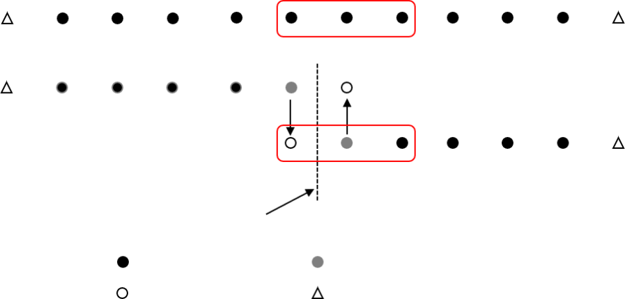
Figure 1: A schematic of a one-dimensional discretized domain in (a) serial and in (b) parallel (bottom) with two processing elements. The red curve denotes the three-point stencil about point $j$ and the dashed line denotes the processor boundary.

In the asynchronous computing method [15], the halo exchanges are initiated, but no explicit synchronization is imposed. Therefore the function value at buffer points may or may not be at the latest time level $n$, which modifies the update equation in Eq. (2) for PE boundary points (assuming that the points are at the left boundary) to

$$\frac{{u_{j}^{n+1}}-u_{j}^{n}}{\Delta t}=\alpha\frac{u_{j+1}^{n}-2u_{j}^{n}+u_{j-1}^{n-\tilde{k}}}{\Delta x^{2}}+\mathcal{O}(\Delta t/\Delta x^{2},\Delta t,\Delta x^{2}),$$ (3)

where $\tilde{k}$ represents the time level delay resulting from the relaxed synchronization. If the communication at the latest time level is complete, then $\tilde{k}=0$ and the computations at the PE boundary points are synchronous (like the interior points). Otherwise, $\tilde{k}>0$ and the update equation would involve a delayed function value, resulting in asynchronous computations. Note that depending on the computation and communication time scales, delays at different PE boundaries can be different and can be several time levels older. Let $\mathcal{L}$ be the maximum allowable delay between the two PEs at a PE boundary. Then, the delay $\tilde{k}\in\left\{0,1,2,\dots,\mathcal{L}-1\right\}$. As the arrival of messages at PE boundaries can be modeled as a random process [29], the corresponding delay values, $\tilde{k}$, take on random values. Let $p_{k}$ represent the probability of occurrence of a $k$ time level delay, i.e. $\tilde{k}=k$, in a simulation. The sum of probabilities is $\sum_{k=0}^{\mathcal{L}-1}p_{k}=1$.

It is evident that the numerical properties of standard schemes used asynchronously would not just depend on numerical and physical parameters such as grid resolution ($\Delta x$), time step ($\Delta t$) and diffusion coefficient ($\alpha$), but would also depend on simulation parameters such as the number of PEs ($\mathcal{P}$), stencil size, delay probabilities ($p_{k}$) and maximum allowable delay ($\mathcal{L}$). A statistical framework was developed in [15] to assess the numerical properties of finite differences implemented with relaxed communication synchronizations. It was shown that asynchronous computations at the PE boundaries would not only affect the stability and consistency of the overall numerical method, but also significantly degrade the accuracy. For the schemes considered in Eq. (3), the truncation error consists of terms that are functions of $\Delta t/\Delta x^{2}$, $\Delta t$ and $\Delta x^{2}$ to leading order. From stability analysis, which gives the relation $\Delta t\sim\Delta x^{2}$ for a constant CFL number, the leading order term is identified as $\mathcal{O}{(\Delta t/\Delta x^{2})}$, which is zeroth-order accurate. Following the analysis described in [15], one can obtain the overall accuracy in the domain to be $\mathcal{O}{(\Delta x)}$ or first-order accurate. It can also be shown that the error would scale linearly with the number of PEs $P$ and mean delay $\bar{\tilde{k}}$. As standard schemes would result in poor accuracy under relaxed data synchronization, new asynchrony-tolerant schemes were derived subsequently [24], which are summarised next.

2.2 Asynchrony-tolerant (AT) spatial schemes

The basic idea of asynchrony-tolerant (AT) schemes is to use an extended stencil in space and/or time to recover loss of accuracy due to the use of delayed data. For example, the spatial derivative of $u_{j}^{n}:=u(j\Delta x,n\Delta t)$ at location $j$ and time level $n$ can be computed using

$$\left.\frac{\partial u}{\partial x}\right|_{j}^{n}=\frac{1}{\Delta x}\sum_{\ell=0}^{\mathcal{L}-1}\sum_{m=-M_{1}(\ell)}^{M_{2}(\ell)}a_{m}^{\ell}u_{j+m}^{n-\ell},$$ (4)

where $\Delta x$ is the grid size, $M_{1}(\ell)$ and $M_{2}(\ell)$ are the extents of stencil to the left and right of $u_{j}^{n}$ and $\mathcal{L}$ is the maximum allowable delay level. For a given set of parameters $\{\mathcal{L},M_{1}(\ell),M_{2}(\ell)\}$ the unknown weights $a_{m}^{\ell}$ are obtained by solving a linear system of equations that is formed by imposing necessary accuracy constraints on terms of the Taylor series expansion of $u_{j+m}^{n-\ell}$ about $u_{j}^{n}$. If $\mathcal{L}=1$ and $M_{1}(0)=M_{2}(0)=M$, this system of equations yields coefficients for the standard central difference scheme. For $\mathcal{L}>1$, AT schemes can be derived if the stencil parameters $\{M_{1}(\ell),M_{2}(\ell)\}$ are appropriately chosen. An example of a second-order AT scheme with $\Delta t\sim\Delta x^{2}$ at the left processor boundary, i.e. delayed data is used only at the left stencil points, is

$$\left.\frac{\partial u}{\partial x}\right|_{j}^{n}=\frac{\tilde{k}u_{j-1}^{n-\tilde{k}-1}-(\tilde{k}+1)u_{j-1}^{n-\tilde{k}}+u_{j+1}}{\Delta x}$$ (5)

where $\tilde{k}$ is the delay [24]. We note that the coefficients in Eq. (5) depend upon delays, unlike the fixed coefficients in standard schemes. Furthermore, in the absence of delays i.e when $\tilde{k}=0$, Eq. (5) reduces to the standard central difference scheme for the first derivative. The general methodology to derive different families of AT schemes of arbitrary order of accuracy is described in [24]. Here the AT schemes from [24] are directly used and are listed in the Appendix without details of the derivation.

2.3 Temporal scheme: Runge-kutta

For a fully-discrete system, the global order of accuracy depends on both the spatial and temporal discretizations. In order to compute this global order, a stability relation of the form $\Delta t\sim\Delta x^{r}$ is used to express the leading order truncation error term of the time discretization scheme also in terms of grid size ($\Delta x$). For example, for a fourth-order spatial scheme ($\mathcal{O}(\Delta x^{4})$), if a second-order temporal discretization scheme ($\mathcal{O}(\Delta t^{2})$) is used then the global spatial order is two if $\Delta t\sim\Delta x$ and four if $\Delta t\sim\Delta x^{2}$. One of the most widely used schemes for high-order temporal discretization is the multi-stage Runge-Kutta (RK) method. An $S$-stage explicit RK scheme for an equation of the form $du/dt=f(u,t)$ over a time step $\Delta t$ is given by

$$u^{n+1}=u^{n}+\Delta t\sum_{s=0}^{S}b_{s}K_{s},$$ (6)

where the stages $K_{s}$ are computed using

$$K_{1} =f(u^{n},t^{n})$$ (7)

$$K_{s} =f(u^{n}+\Delta t\sum_{i=1}^{s-1}(a_{si}k_{i}),t^{n}+c_{s}\Delta t).$$

Here $a_{si},b_{s},c_{s}$ are the coefficients of the RK scheme. For an RK scheme, in advancing from time level $n$ to $n+1$, intermediate stages $K_{s}$ are computed. Each of these stages depends upon the previous stages as can be seen from Eq. (7). Thus, for simulations performed in parallel, RK schemes require PEs to communicate and synchronize after every stage in order to update the corresponding values at buffer points. However, if simulations are performed with asynchronous communications using AT schemes, then a fractional delay will be encountered at the intermediate stages and different AT schemes will be required for each stage. An alternate method is proposed to effectively use multi-stage RK schemes with AT that circumvents the need to communicate at every stage and avoids fractional delays.

In the presence of delays, each stage $K_{s}$ is computed using AT schemes at PE boundary points. As mentioned before, the current stage $K_{s}$ explicitly depends upon the previous stages, $K_{s-1},K_{s-2},\dots,K_{1}$. Thus, to ensure accuracy all the stages of RK scheme are computed locally at both PE boundary and buffer points of each PE. Furthermore, at the old time levels required by the AT scheme, these stages are also computed at the internal points close to the PE boundary. In order to perform the additional computations at buffer points, a larger message of size (= No. of stages in RK $\times$ spatial stencil) has to be communicated across processors at every time step. However, the PEs no longer communicate at every stage of the RK. Thus, there exists a trade-off between communication which is expensive and computation which is relatively cheap.

To illustrate that the RK schemes preserve the order of accuracy when combined with high-order AT schemes, the one-dimensional diffusion equation in Eq. (1) is reconsidered. Denoting the right-hand-side of Eq. (1) by $f(u,t)=\partial^{2}u/\partial x^{2}$ (excluding the diffusion coefficient, $\alpha$), the temporal discretization at the $j$-th spatial point using a two-stage second-order RK scheme (RK2) is given by

$$u_{j}^{n+1}=u_{j}^{n}+\alpha\Delta t\left(\frac{K_{j,1}}{2}+\frac{K_{j,2}}{2}\right)$$ (8)

where $K_{j,1}=f(u_{j}^{n},t^{n})$, $K_{j,2}=f\left((u_{j}^{n})^{*},t^{n}+\Delta t\right)$ and $(u_{j}^{n})^{*}=u_{j}^{n}+\Delta t(f(u_{j}^{n},t^{n}))=u_{j}^{n}+\Delta t\alpha K_{j,1}$. When a standard fourth-order central difference scheme is used for numerical approximation of $f(u_{j}^{n},t^{n})$, the following $K_{j,1}$ and $K_{j,2}$ are obtained,

$$K_{j,1}= \frac{-u_{j-2}^{n}+16u_{j-1}^{n}-30u_{j}^{n}+16u_{j+1}^{n}-u_{j+2}^{n}}{12\Delta x^{2}}$$ (9)

$$K_{j,2}= -\frac{\alpha\Delta t(K_{j-2,1})+u_{j-2}^{n}}{12\Delta x^{2}}+\frac{4\left(\alpha\Delta t(K_{j-1,1})+u_{j-1}^{n}\right)}{3\Delta x^{2}}-\frac{5\left(\alpha\Delta t\left(K_{j,1}\right)+u_{j}^{n}\right)}{2\Delta x^{2}}$$

$$+\frac{4\left(\alpha\Delta t(K_{j+1,1})+u_{j+1}^{n}\right)}{3\Delta x^{2}}-\frac{\alpha\Delta t\left(K_{j+2,1}\right)+u_{j+2}^{n}}{12\Delta x^{2}}.$$

The Taylor series expansion of Eq. (8) on substituting Eq. (9) then yields a truncation error of the form

$$\text{TE}_{j}^{n}|_{\text{sync}}=\frac{1}{6}\left(-f^{(0,3)}(x,t)\right)\Delta t^{2}-\frac{1}{90}\alpha f^{(6,0)}(x,t)\Delta x^{4}+\mathcal{O}(\Delta x^{6},\Delta t^{3},\Delta x^{4}\Delta t)$$ (10)

or

$$\text{TE}_{j}^{n}|_{\text{sync}}=(-\frac{r_{\alpha}^{2}u^{(0,3)}(x,t)}{6\alpha^{2}}-\frac{1}{90}\alpha u^{(6,0)}(x,t))\Delta x^{4}+\mathcal{O}(\Delta x^{6}),$$ (11)

where $r_{\alpha}=\alpha\Delta t/\Delta x^{2}$ is the diffusive CFL number and the subscript “sync” denotes synchronous. Note that from Eq. (11) the global spatial order of accuracy is four.

When a fourth-order AT scheme is used at the boundary points for computation of spatial derivatives, we have

$$K_{j,1}= \left(\tilde{k}^{2}+\tilde{k}\right)\frac{\left(-u_{j-2}^{n-\tilde{k}-2}+16u_{j-1}^{n-\tilde{k}-2}-30u_{j}^{n}+16u_{j+1}^{n}-u_{j+2}^{n}\right)}{24\Delta x^{2}}$$ (12)

$$-\left(\tilde{k}^{2}+2\tilde{k}\right)\frac{\left(-u_{j-2}^{n-\tilde{k}-1}+16u_{j-1}^{n-\tilde{k}-1}-30u_{j}^{n}+16u_{j+1}^{n}-u_{j+2}^{n}\right)}{12\Delta x^{2}}$$

$$+\left(\tilde{k}^{2}+3\tilde{k}+2\right)\frac{\left(-u_{j-2}^{n-\tilde{k}}+16u_{j-1}^{n-\tilde{k}}-30u_{j}^{n}+16u_{j+1}^{n}-u_{j+2}^{n}\right)}{24\Delta x^{2}}$$

which is used to compute $K_{j,2}=f(u_{j}^{n}+\Delta t\alpha K_{j,1},t^{n}+\Delta t)$ with $f(.,.)$ being evaluated using the fourth-order AT-scheme as well. Once again, the Taylor series expansion is used to obtain the truncation error,

$$\text{TE}_{j}^{n}|_{\text{AT},\tilde{k}}=-\frac{5}{24}\alpha\tilde{k}\left(\tilde{k}^{2}+3\tilde{k}+2\right)u^{(0,3)}(x,t)\frac{\Delta t^{3}}{\Delta x^{2}}-\frac{1}{6}u^{(0,3)}(x,t)\Delta t^{2}-\frac{1}{90}\alpha u^{(6,0)}(x,t)\Delta x^{4}+\mathcal{O}(\tilde{k}^{3}\frac{\Delta t^{3}}{\Delta x}).$$ (13)

The above expression simplifies to give a global fourth-order truncation error term when $r_{\alpha}$ is substituted,

$$\text{TE}_{j}^{n}|_{\text{AT},\tilde{k}}=-\left(\frac{75\tilde{k}\left(\tilde{k}^{2}+3\tilde{k}+2\right)r_{\alpha}^{3}u^{(0,3)}(x,t)+60r_{\alpha}^{2}u^{(0,3)}(x,t)+4\alpha^{3}u^{(6,0)}(x,t)}{360\alpha^{2}}\right)\Delta x^{4}+\mathcal{O}(\Delta x^{6}).$$ (14)

When the delay is zero i.e. $\tilde{k}=0$, the truncation error in Eq. (14) reduces to $\text{TE}_{j}^{n}|_{\text{sync}}$ (Eq. (11)) which is the synchronous truncation error at the internal points. Therefore, RK schemes can be used with the AT-schemes without affecting the global order of accuracy. During a simulation the stencil data at older time levels for the buffer as well as for internal points are available, and hence standard synchronous schemes can be used to compute the sub-stages $K_{j,s}$ at these points for efficient implementation of RK with AT. Numerical simulations of linear equations were performed using this approach and the global order of accuracy was preserved. Here the order of accuracy tests are shown for RK schemes with AT-WENO schemes that are derived next (see Table 1).

3 Asynchrony-tolerant Weighted Essentially Non-oscillatory schemes (AT-WENO)

Despite their advantages, central finite difference schemes are not always suitable for performing DNS of, for example, supersonic flows. In the presence of sharp gradients or discontinuities in density, temperature and composition due to detonations, shocks or high pressure flames, the central difference schemes are prone to numerical oscillations and instabilities. A well established numerical technique to accurately simulate flows with piece-wise smooth solutions between discontinuities is the so called weighted essentially non-oscillatory schemes (WENO) [30, 31]. These schemes aim to achieve high-order accuracy at the smooth regions of the flow and resolve the discontinuities with minimal oscillations by automatically selecting the locally smoothest stencil. WENO schemes are considerably more expensive than regular central difference schemes due to the need to evaluate the same flux functions from multiple candidate stencils [32]. However, the numerical method is suitable for implementation in finite difference codes using stencil operations very similar to the central difference schemes. Also, the usual advantages of DNS using finite difference schemes including parallelism and scalability apply to the WENO schemes as well. Apart from DNS [33, 12], the advantages of WENO schemes have also been demonstrated in implicit large eddy simulations (iLES) [34, 35, 36].

In this section, a brief overview of the standard WENO schemes is provided followed by a discussion on the effect of asynchrony on the standard WENO schemes (AS-WENO) and derivation of the asynchrony-tolerant WENO (AT-WENO) schemes for accurate numerical simulations when delays are observed at PE boundaries. Consider the one-dimensional ($x$-direction) version of the governing equations:

$$\frac{\partial Q}{\partial t}+\frac{\partial C}{\partial x}+\frac{\partial D}{\partial x}=S,$$ (15)

where $Q$ is the solution vector, $C$ is the vector comprising the convective flux terms, $D$ is the viscous and molecular diffusion flux vector, and $S$ is the vector of source terms. The exact form of terms in $Q,C$ and $D$ is defined in section 4. In the WENO framework, the terms contained in the $D$ vector do not require any special treatment and are evaluated using central difference schemes (standard or AT). However, the convective flux terms in $C$ have to be computed appropriately to ensure both stability and accuracy in regions near and at discontinuities. Specifically, the derivative of the convective flux $\partial C/\partial x$ at a point $j$ is approximated using the flux at the edges, i.e., $\widehat{C}_{j\pm\frac{1}{2}}$ of a cell $\mathcal{I}_{j}=[x_{j-\frac{1}{2}},x_{j+\frac{1}{2}}]$. The flux at the edges is computed using the WENO approximation procedure that can be carried out using interpolation or reconstruction, and accordingly, requires point values or cell averages of the fluxes. Note that the hat notation $(~{}\widehat{}~{})$ is used to denote the variables at cell edges. The derivative is then computed using the relation

$$\left.\frac{\partial C}{\partial{x}}\right|_{j}=\frac{\widehat{C}_{j+\frac{1}{2}}-\widehat{C}_{j-\frac{1}{2}}}{\Delta x}$$ (16)

for a uniform grid and the order depends upon the order of the numerical flux approximation $\widehat{C}_{j\pm\frac{1}{2}}$. When using finite-differences, the WENO approximation directly yields the fluxes at the edges in terms of the fluxes at the grid points. For stability, appropriate up-winding of fluxes is also required and is achieved through splitting the flux, for example using the local Lax-Friedrichs flux splitting methodology,

$$C=C^{+}+C^{-},\quad\text{where}$$ (17)

$$C^{\pm}=\frac{1}{2}(C\pm\lambda_{max}Q),$$

at every grid-point. The quantity $\lambda_{max}$ in Eq. (17) is the maximum local wave propagation speed which can be computed as

$$\left.\lambda_{max}\right|_{j}=\max\{(|u|)_{j-1},(|u\pm c|)_{j-1},(|u|)_{j},(|u\pm c|)_{j}\},$$ (18)

where $u$ and $c$ are the local flow velocity and the speed of sound, respectively. The derivative is then simply evaluated using

$$\left.\frac{\partial C}{\partial x}\right|_{j}=\frac{\widehat{C}^{+}_{j+\frac{1}{2}}-\widehat{C}^{+}_{j-\frac{1}{2}}}{\Delta x}+\frac{\widehat{C}^{-}_{j+\frac{1}{2}}-\widehat{C}^{-}_{j-\frac{1}{2}}}{\Delta x}$$ (19)

with an appropriate upwind stencil for approximating both positive and negative fluxes [12]. For computation of derivative in Eq. (19) using the WENO procedure, the first step is to approximate the fluxes at the edges ($j\pm 1/2$) through an interpolation or a reconstruction procedure. For simplicity, the approximation of these fluxes using an interpolation technique is discussed here in detail. However, the approximation through reconstruction that treats grid-point values as cell averages can also be performed following the steps detailed here. In order to do so, the primitive function defined in [30] is required.

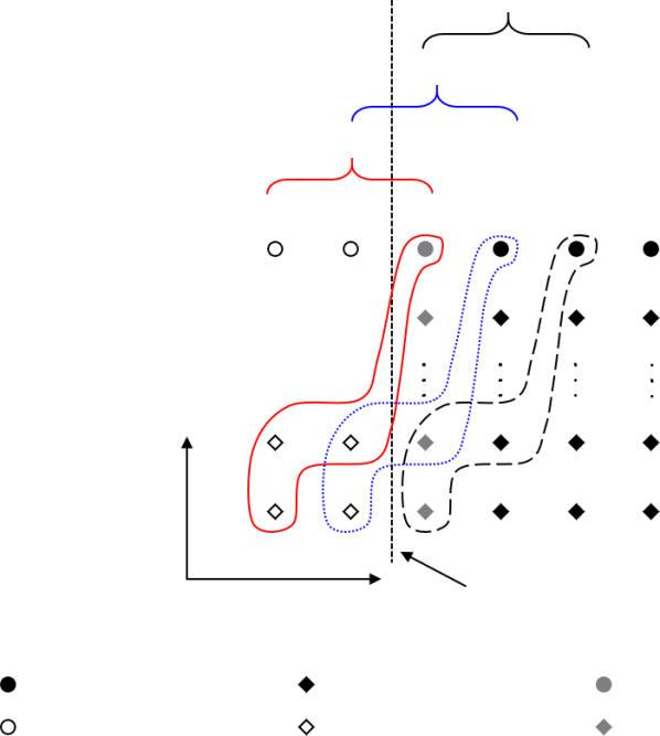
Figure 2: Four-point candidate stencils for asynchronous WENO approximation at the left processor boundary. $S^{(0)},S^{(1)}$ and $S^{(2)}$ are the three-point candidate synchronous WENO stencils for approximation at point $j+1/2$ and the corresponding curves are the AT candidate stencil with delays on the left.

For illustration, consider a specific WENO scheme that uses three sub-stencils each of which comprises three grid-points denoted by $S^{(i)}$, $i=\{0,1,2\}$, in Fig. 2 to approximate the value of a quantity $\hat{u}$ at cell edges, say $j+1/2$, and time-level $n$. Taken together the larger stencil obtained by combining these $S^{(i)}$ contains five points. Since the approximation order depends upon the number of points, a fifth-order accurate approximation can be obtained with the full stencil for a smooth function. This is the classical three-fifth order WENO scheme, where the three smaller candidate stencils $S^{(0)}=\{j-2,j-1,j\}$, $S^{(1)}=\{j-1,j,j+1\}$, and $S^{(2)}=\{j,j+1,j+2\}$ give a degree two polynomial interpolation of $\hat{u}_{j+\frac{1}{2}}^{n}$ at time level $n$. The synchronous third-order interpolant in each of the three stencils can be computed using Taylor series expansion or Lagrange interpolation [30, 31],

$$\hat{u}_{j+\frac{1}{2}}^{n,(0)}=\frac{3}{8}u_{j-2}^{n}-\frac{5}{4}u_{j-1}^{n}+\frac{15}{8}u_{j}^{n}+\mathcal{O}(\Delta x^{3})$$ (20)

$$\hat{u}_{j+\frac{1}{2}}^{n,(1)}=-\frac{1}{8}u_{j-1}^{n}+\frac{3}{4}u_{j}^{n}+\frac{3}{8}u_{j+1}^{n}+\mathcal{O}(\Delta x^{3})$$

$$\hat{u}_{j+\frac{1}{2}}^{n,(2)}=\frac{3}{8}u_{j}^{n}+\frac{3}{4}u_{j+1}^{n}-\frac{1}{8}u_{j+2}^{n}+\mathcal{O}(\Delta x^{3}).$$

The final approximation is taken as a convex combination of the above three third-order approximations, yielding a higher order interpolant in the larger stencil. Ideally, if $u(x,t)$ is smooth in the large stencil $S=\bigcup\limits_{i=0}^{2}S^{(i)}=\{j-2,j-1,j,j+1,j+2\}$, a fifth-order approximation can be achieved using the following expression:

$$\hat{u}_{j+\frac{1}{2}}^{n}=\sum_{i=0}^{2}\omega_{i}\hat{u}_{j+\frac{1}{2}}^{n,(i)},$$ (21)

where $\omega_{i}$’s are the non-linear weights

$$\omega_{i}=\frac{\alpha_{i}}{\sum\limits_{i=0}^{2}\alpha_{i}},\quad\alpha_{i}=\frac{\gamma_{i}}{(\epsilon+\beta^{(i)})^{2}}.$$ (22)

The non-linear weights in Eq. (22) satisfy $w_{i}\geq 0$ and $\sum\limits_{i=0}^{2}\omega_{i}=1$ and are related to the ideal or linear weights $\gamma_{i}$ through the smoothness indicator $\beta^{(i)}$ [37, 31, 38]. A simple Taylor series expansion yields the ideal weights $\gamma=\{\frac{1}{16},\frac{5}{8},\frac{5}{16}\}$, such that

$$\hat{u}_{j+\frac{1}{2}}^{n}=\frac{3}{128}u_{j-2}^{n}-\frac{5}{32}u_{j-1}^{n}+\frac{45}{64}u_{j}^{n}+\frac{15}{32}u_{j+1}^{n}-\frac{5}{128}u_{j+2}^{n}+\mathcal{O}(\Delta x^{5}).$$ (23)

We now focus on the effect of data asynchrony on each of the individual approximations. Consider a point $j$ at the left processor boundary with a delay $\tilde{k}$ encountered at each of the buffer points. The order of accuracy of the interpolants in the first two stencils is affected by this delay,

$$\hat{u}_{j+\frac{1}{2}}^{n,(0)}=\frac{3}{8}u_{j-2}^{n-\tilde{k}}-\frac{5}{4}u_{j-1}^{n-\tilde{k}}+\frac{15}{8}u_{j}^{n}+\mathcal{O}(\Delta t,\Delta x\Delta t,\Delta x^{3})$$ (24)

$$\hat{u}_{j+\frac{1}{2}}^{n,(1)}=-\frac{1}{8}u_{j-1}^{n-\tilde{k}}+\frac{3}{4}u_{j}^{n}+\frac{3}{8}u_{j+1}^{n}+\mathcal{O}(\Delta t,\Delta x\Delta t,\Delta x^{3}).$$

More precisely, there are terms in the truncation error that depend upon $\Delta t$. On relating $\Delta t\sim\Delta x^{r}$, the interpolants with delays reduce to first order when $r=1$ (convective CFL) and to second order when $r=2$ (diffusive CFL). The convex combination of the three interpolants with ideal weights $\gamma_{i}$ also has a leading order truncation term that scales as $\mathcal{O}(\Delta t)$, thereby degrading the order even in the full stencil, i.e

$$\hat{u}_{j+\frac{1}{2}}^{n}=\frac{3}{128}u_{j-2}^{n-\tilde{k}}-\frac{5}{32}u_{j-1}^{n-\tilde{k}}+\frac{45}{64}u_{j}^{n}+\frac{15}{32}u_{j-1}^{n}-\frac{5}{128}u_{j+2}^{n}+\mathcal{O}(\Delta t,\Delta x\Delta t,\Delta t^{2},\Delta x^{2}\Delta t).$$ (25)

Clearly, the standard interpolants cannot be used in the presence of delays. A similar degradation in order was observed when standard finite difference schemes are used with asynchrony [15] for computation of spatial derivatives. Following the general methodology to overcome this loss of accuracy in [24], the asynchrony-tolerant WENO schemes (AT-WENO) can be derived. For this, the AT-interpolant for each of the substencils in the presence of delays is computed. When multiple time-levels are used, the interpolation is two-dimensional i.e. in space and time, and thus, requires a greater numbers of points to achieve a given order of accuracy. Since the Taylor series expansion is used to obtain the coefficients, a relation of the form $\Delta t\sim\Delta x^{r}$ is also needed to identify the overall low-order terms (in space) that should be eliminated for achieving the desired order of accuracy. A schematic representation to identify low-order terms which need to be subjected to constraints is illustrated in Figures 2 and 3 in [24]. For example, for a third-order accurate approximation, when $\Delta t\sim\Delta x$, six equations corresponding to terms of the order $\{1,\Delta t,\Delta x,\Delta t^{2},\Delta t\Delta x,\Delta x^{2}\}$ are needed, and therefore, each candidate stencil comprises six points. Similarly, if $r=2$ only four equations $\{1,\Delta t,\Delta x,\Delta x^{2}\}$ are required, and therefore, a four-point stencil is sufficient to achieve a third-order approximation. Since the stencil now depends upon the delays observed at the processor boundaries, the stencil itself is random because of the random nature of the delays. One can represent this stochastic stencil as $\tilde{S}$. For the first candidate stencil (as shown in Fig. 2), $\tilde{S}^{(0)}=\{u_{j-2}^{-\tilde{k}+n-1},u_{j-2}^{n-\tilde{k}},u_{j-1}^{n-\tilde{k}},u_{j}^{n}\}$ with delay $\tilde{k}$ and $r=2$, the AT interpolant is

$$\tilde{u}_{j+\frac{1}{2}}^{n,(0)}=\frac{7}{8}\tilde{k}u_{j-2}^{-\tilde{k}+n-1}+\frac{1}{8}\left(3-7\tilde{k}\right)u_{j-2}^{n-\tilde{k}}-\frac{5}{4}u_{j-1}^{n-\tilde{k}}+\frac{15}{8}u_{j}^{n}+\text{TE}^{(0)}.$$ (26)

The leading order truncation error in Eq. (26) term depends on the delay $\tilde{k}$ and is equal to

$$\text{TE}^{(0)}=\frac{-5}{4}\tilde{k}\dot{u}^{\prime}(x,t)\Delta t\Delta x+\frac{5}{16}u^{\prime\prime\prime}(x,t)\Delta x^{3}+\dots\sim\mathcal{O}(\Delta x^{3}),$$ (27)

where $\dot{u}=\partial u/\partial t$ and $u^{\prime}=\partial u/\partial x$ and $\Delta t\sim\Delta x^{2}$ gives the overall spatial order of accuracy to be $\mathcal{O}(\Delta x^{3})$. When $\tilde{k}=0$, Eq. (26) reduces to the standard third-order synchronous interpolant in Eq. (20). For the second stencil $\tilde{S}^{(1)}=\{u_{j-1}^{-\tilde{k}+n-1},u_{j-1}^{-\tilde{k}},u_{j}^{n},u_{j+1}^{n}\}$, with delays considered only at the buffer point ($u_{j-1}$), the third-order interpolant is

$$\tilde{u}_{j+\frac{1}{2}}^{n,(1)}=\frac{1}{8}\tilde{k}u_{j-1}^{-\tilde{k}+n-1}+\frac{1}{8}\left(-\tilde{k}-1\right)u_{j-1}^{n-\tilde{k}}+\frac{3}{4}u_{j}^{n}+\frac{3}{8}u_{j+1}^{n}+\text{TE}^{(1)},$$ (28)

where the leading order truncation error term

$$\text{TE}^{(1)}=-\frac{1}{16}u^{\prime\prime\prime}(x,t)\Delta x^{3}+\dots\sim\mathcal{O}(\Delta x^{3})$$ (29)

is independent of delay $\tilde{k}$, unlike Eq. (27). Lastly, for stencil $\tilde{S}^{(2)}=\{u_{j}^{n},u_{j+1}^{n},u_{j+2}^{n}\}=S^{(2)}$, since all the points are within the PE, the standard interpolant i.e. $\tilde{u}_{j+\frac{1}{2}}^{n,(2)}=\hat{u}_{j+\frac{1}{2}}^{n,(2)}$ can readily be used. The full stencil is comprised of seven points $\tilde{S}=\bigcup\limits_{i=0}^{2}\tilde{S}^{(i)}=\{u_{j-2}^{-\tilde{k}+n-1},u_{j-2}^{n-\tilde{k}},u_{j-1}^{-\tilde{k}+n-1},u_{j-1}^{n-\tilde{k}},u_{j}^{n},u_{j+1}^{n},u_{j+2}^{n}\}$. With this choice of stencil, at most, a fourth-order accurate approximation can be obtained for the full stencil since the degrees of freedom are sufficient only to eliminate seven low-order terms. Extension to higher orders would require extending the stencil in both space and time. This is explained in great detail in [24] for AT finite difference schemes.

On evaluation of the ideal weights for this larger stochastic stencil $\tilde{S}$ i.e.

$$\tilde{u}_{j+\frac{1}{2}}^{n}=\sum_{i=0}^{2}\gamma_{i}\tilde{u}_{j+\frac{1}{2}}^{n,(i)},$$ (30)

yields

$$\gamma=\left\{0,\frac{1}{2},\frac{1}{2}\right\}$$ (31)

which, in turn, gives a fourth-order truncation error term in Eq. (30). These ideal weights eliminate the first stencil $\tilde{S}^{(0)}$ and reduce the full stencil to a four-point synchronous stencil in the absence of delays. If the second stencil is modified $\tilde{S}^{(1)}=\{u_{j-1}^{-\tilde{k}+n-1},u_{j-1}^{n-\tilde{k}},u_{j}^{n-\tilde{k}},u_{j+1}^{n}\}$, the ideal weights are no longer positive, $\gamma=\left\{-\frac{3}{2},-\frac{5}{2},5\right\}.$ Further changing the third stencil to $\tilde{S}^{(2)}=\{u_{j}^{-\tilde{k}+n-1},u_{j}^{n-\tilde{k}},u_{j+1}^{n-\tilde{k}},u_{j+2}^{n}\}$ such that all three stencils now have similar stencil structure and thus use four points as shown in Fig. 2, the ideal weights obtained are

$$\gamma=\left\{\frac{3}{8},\frac{5}{4},-\frac{5}{8}\right\}.$$ (32)

This exercise shows that irrespective of the choice of asynchronous stencil with four points, at least one of the ideal or linear weights is non-positive for integer values of $\tilde{k}$. This non-convex nature of ideal weights leads to instabilities and oscillations [39]. The procedure to deal with the non-positive weights has been described in [39] and it involves splitting all the weights into positive and negative parts,

$$\tilde{\gamma}_{i}^{+}=\frac{1}{2}\left(\gamma_{i}+\theta|\gamma_{i}|\right)$$ (33)

$$\tilde{\gamma}_{i}^{-}=\tilde{\gamma}_{i}^{+}-\gamma_{i}$$

for $i=\{0,1,2\}$. The split ideal weights are then scaled by the parameters

$$\sigma^{\pm}=\sum_{i=1}^{3}\tilde{\gamma}_{i}^{\pm};\quad\gamma_{i}^{\pm}=\tilde{\gamma}_{i}^{+}/\sigma^{\pm},$$ (34)

which are used to write the split polynomial interpolations

$$\left(\hat{u}_{j+\frac{1}{2}}^{n}\right)^{\pm}=\sum_{i=0}^{2}\gamma_{i}^{\pm}\hat{u}_{j+\frac{1}{2}}^{n,(i)},$$ (35)

which is equivalent to replacing the ideal positive weight $\gamma_{i}$ in Eq. (22) by the corresponding scaled split weight $\gamma^{\pm}_{i}$ [39]. However, this procedure does involve a series of additional computations to compute the derivative of the flux accurately.

For this particular choice of stencil with delayed data at the left boundaries, the reconstruction polynomial can also be derived using the primitive function [30]. For example, for a stencil of the form $\tilde{S}^{(i)}=\{u_{j-1+i}^{-\tilde{k}+n-1},u_{j+i}^{n-\tilde{k}},u_{j+1+i}^{n-\tilde{k}},u_{j+1+i}^{n}\}$ where $i=\{0,1,2\}$, one obtains the following AT approximations,

$$\tilde{u}^{n,(i)}_{j+\frac{1}{2}}= \frac{1}{6}\left(3i^{2}-12i+5\right)\tilde{k}u_{i+j-2}^{-\tilde{k}+n-1}+\frac{1}{6}\left(-3i^{2}\tilde{k}+12i\tilde{k}-5\tilde{k}+3i^{2}-6i+2\right)u_{i+j-2}^{n-\tilde{k}}$$ (36)

$$+\frac{1}{6}\left(-6i^{2}+18i-7\right)u_{i+j-1}^{n-\tilde{k}}+\frac{1}{6}\left(3i^{2}-12i+11\right)u_{i+j}^{n}.$$

The reconstruction polynomials in Eq. (36) reduce to the traditional candidate reconstruction polynomials in [38, 30] when $\tilde{k}=0$ for three-fifth order WENO scheme with ideal weights $\{1/10,6/10,3/10\}$.

As is evident from Eq. (22), the non-linear weights $\omega_{i}$ that are integral to the WENO formulation depend upon the smoothness indicators $\beta_{i}$ defined in [30] as

$$\beta^{(i)}=\sum_{\ell=1}^{k}\Delta x^{2\ell-1}\int_{x_{j-\frac{1}{2}}}^{x_{j+\frac{1}{2}}}\left(\frac{d^{\ell}}{dx^{\ell}}p^{(i)}(x)\right)^{2}dx$$ (37)

where $p^{(i)}(x)$ is the polynomial of degree $k$ (=2, in the example considered here) for stencil $S^{(i)}$. For a one-dimensional polynomial interpolation Eq. (37) can be easily evaluated to give a smoothness indicator for each stencil. However, for a simpler extension to an asynchronous stencil, Simpson’s 3/8 rule is used to compute $\beta^{(i)}$,

$$\beta^{(i)}=\frac{\Delta x}{6} \Bigg{(}\sum_{\ell=1}^{k}\Delta x^{2\ell-1}\Bigg{(}\left.\frac{d^{\ell}}{dx^{\ell}}p^{(j)}(x)\right|_{x=x_{j-\frac{1}{2}}}\Bigg{)}^{2}+4\sum_{\ell=1}^{k}\Delta x^{2\ell-1}\Bigg{(}\left.\frac{d^{\ell}}{dx^{\ell}}p^{(j)}(x)\right|_{x=x_{j-\frac{1}{6}}}\Bigg{)}^{2}$$ (38)

$$+4\sum_{\ell=1}^{k}\Delta x^{2\ell-1}\Bigg{(}\left.\frac{d^{\ell}}{dx^{\ell}}p^{(j)}(x)\right|_{x=x_{j+\frac{1}{6}}}\Bigg{)}^{2}+\sum_{\ell=1}^{k}\Delta x^{2\ell-1}\Bigg{(}\left.\frac{d^{\ell}}{dx^{\ell}}p^{(j)}(x)\right|_{x=x_{j+\frac{1}{2}}}\Bigg{)}^{2}\Bigg{)},$$

such that the derivatives of the interpolant are computed numerically at each of $\{x_{j-\frac{1}{2}},x_{j-\frac{1}{6}},x_{j+\frac{1}{6}},x_{j+\frac{1}{2}}\}$ using all the points in the stencil $S^{(i)}$. This yields the smoothness indicator expressed in the form

$$\beta^{(0)}=\frac{1}{3}\left(4\left(u^{n}\right)_{j-2}^{2}+\left(11u^{n}_{j}-19u^{n}_{j-1}\right)u^{n}_{j-2}+25\left(u^{n}\right)_{j-1}^{2}+10\left(u^{n}\right)_{j}^{2}-31u^{n}_{j-1}u^{n}_{j}\right)$$ (39)

$$\beta^{(1)}=\frac{1}{3}\left(4\left(u^{n}\right)_{j-1}^{2}+\left(5u^{n}_{j+1}-13u^{n}_{j}\right)u^{n}_{j-1}+13\left(u^{n}\right)_{j}^{2}+4\left(u^{n}\right)_{j+1}^{2}-13u^{n}_{j}u^{n}_{j+1}\right)$$

$$\beta^{(2)}=\frac{1}{3}\left(10\left(u^{n}\right)_{j}^{2}+\left(11u^{n}_{j+2}-31u^{n}_{j+1}\right)u^{n}_{j}+25\left(u^{n}\right)_{j+1}^{2}+4\left(u^{n}\right)_{j+2}^{2}-19u^{n}_{j+1}u^{n}_{j+2}\right)$$

which is consistent with $\beta^{(j)}$ in the literature. Extending this to the asynchronous stencil, the smoothness indicator of the following form is obtained when a four-point stencil is used for all three candidate stencils,

$$\tilde{\beta}^{(0)}=\frac{1}{3} \Bigg{(}\left(10\tilde{k}^{2}-11\tilde{k}+4\right)\left(u_{j-2}^{n-\tilde{k}}\right)^{2}+\Big{(}-20\tilde{k}^{2}u_{j-2}^{n-\tilde{k}-1}+\tilde{k}\left(11u_{j-2}^{n-\tilde{k}-1}+31u_{j-1}^{n-\tilde{k}}-20u_{j}^{n}\right)-19u_{j-1}^{n-\tilde{k}}$$ (40)

$$+11u_{j}^{n}\Big{)}u_{j-2}^{n-\tilde{k}}+10\tilde{k}^{2}\left(u_{j-2}^{n-\tilde{k}-1}\right)^{2}+25\left(u_{j-1}^{n-\tilde{k}}\right)^{2}-31u_{j}^{n}u_{j-1}^{n-\tilde{k}}+\tilde{k}u_{j-2}^{n-\tilde{k}-1}\left(20u_{j}^{n}-31u_{j-1}^{n-\tilde{k}}\right)+10\left(u_{j}^{n}\right)^{2}\Bigg{)}$$

$$\tilde{\beta}^{(1)}=\frac{1}{3} \Bigg{(}\left(4\tilde{k}^{2}-5\tilde{k}+4\right)\left(u_{j-1}^{n-\tilde{k}}\right)^{2}+\Big{(}-8\tilde{k}^{2}u_{j-1}^{n-\tilde{k}-1}+\tilde{k}\left(5u_{j-1}^{n-\tilde{k}-1}+13u_{j}^{n-\tilde{k}}-8u_{j+1}^{n}\right)-13u_{j}^{n-\tilde{k}}$$ (41)

$$+5u_{j+1}^{n}\Big{)}u_{j-1}^{n-\tilde{k}}+4\tilde{k}^{2}\left(u_{j-1}^{n-\tilde{k}-1}\right)^{2}+13\left(u_{j}^{n-\tilde{k}}\right)^{2}-13u_{j+1}^{n}u_{j}^{n-\tilde{k}}$$

$$+\tilde{k}u_{j-1}^{n-\tilde{k}-1}\left(8u_{j+1}^{n}-13u_{j}^{n-\tilde{k}}\right)+4\left(u_{j+1}^{n}\right)^{2}\Bigg{)}$$

$$\tilde{\beta}^{(2)}=\frac{1}{3} \Bigg{(}\left(4\tilde{k}^{2}-11\tilde{k}+10\right)\left(u_{j}^{n-\tilde{k}}\right)^{2}+\Big{(}-8\tilde{k}^{2}u_{j}^{n-\tilde{k}-1}+\tilde{k}\left(11u_{j}^{n-\tilde{k}-1}+19u_{j+1}^{n-\tilde{k}}-8u_{j+2}^{n}\right)-31u_{j+1}^{n-\tilde{k}}+11u_{j+2}^{n}\Big{)}$$ (42)

$$u_{j}^{n-\tilde{k}}+4\tilde{k}^{2}\left(u_{j}^{n-\tilde{k}-1}\right)^{2}+25\left(u_{j+1}^{n-\tilde{k}}\right)^{2}-19u_{j+2}^{n}u_{j+1}^{n-\tilde{k}}+\tilde{k}u_{j}^{n-\tilde{k}-1}\left(8u_{j+2}^{n}-19u_{j+1}^{n-\tilde{k}}\right)+4\left(u_{j+2}^{n}\right)^{2}\Bigg{)}.$$

Each of the $\tilde{\beta}^{i}$ listed in Eq. (40), Eq. (41), Eq. (42) reduce to the corresponding $\beta^{(j)}$ expressions in Eq. (39) when $\tilde{k}=0$. With the approximations and smoothness indicators in the candidate stencil known along with the ideal weights, the derivative of the flux can then be computed using the standard WENO procedure.

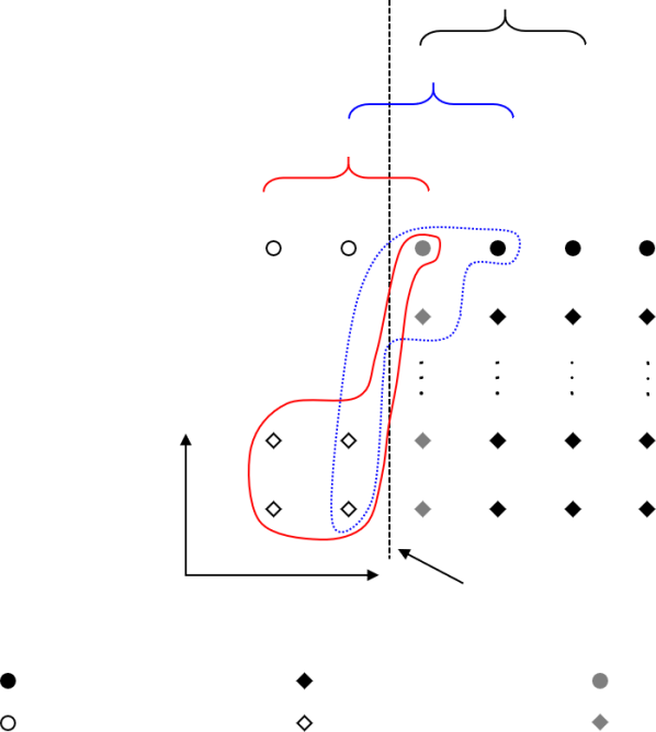
Figure 3: Updated stencil for WENO at the left processor boundary.

For the choice of stencil discussed above, if the delay is zero then instead of achieving fifth-order approximation in the larger stencil, only fourth-order accuracy is obtained. This is explained as follows. The ideal weights $\{\gamma_{0},\gamma_{1},\gamma_{2}\}$ in Eq. (30) satisfy $\sum_{i=0}^{2}\gamma_{i}=1$ and thus, two additional constraints need to be imposed to find a unique solution when seeking a combination of smaller stencils. Upon upgrading from a third-order approximation in the smaller stencil $\tilde{S}^{(j)}$ to a fourth-order approximation in the full stencil $\tilde{S}$, only two lower order truncation error terms of the form $\{\Delta t\Delta x,\Delta x^{3}\}$ can be eliminated. Thus, a unique solution for $\gamma_{i}$ is obtained. However, such an approximation will never recover fifth-order accuracy in the absence of delays since the $\Delta x^{4}$ truncation error term is non-zero. Consequently, when there is no delay, the large stencil $\tilde{S}$ will have at most four points and the approximation is only fourth-order accurate. For example, the ideal weights Eq. (32) yield non-zero coefficients only for points $\{j-2,j-1,j,j+2\}$ in the full stencil when $\tilde{k}=0$. Moreover, this stencil is spatially discontinuous.

The reduction in the number of points in the larger stencil when the delay is zero and a corresponding lower order accurate approximation can be overcome by selectively eliminating additional truncation error terms. For an asynchronous fifth-order approximation, terms of the form $\{\Delta t^{2},\Delta t\Delta x^{2},\Delta x^{4}\}$ in addition to $\{\Delta t\Delta x,\Delta x^{3}\}$ also need to be eliminated. Since this yields a system with six constraints and only three unknowns, a unique solution cannot be determined. However, it is still possible to achieve a fifth-order approximation in the absence of delays. Addition of one more point in the smaller asynchronous stencil and using this degree of freedom to eliminate the $\Delta t\Delta x$ truncation term does not affect the order of the resulting interpolant. However, when the ideal weights in the large stencil are computed, one of the constraints can now be imposed on the $\Delta x^{4}$ term. This exercise then yields convex ideal weights that are exactly equal to the ones obtained when all three small stencils are synchronous. While the asynchronous approximation in the full stencil is still of order four, the synchronous approximation recovers fifth-order accuracy when the delay goes to zero. Moreover, a convex combination of the candidate stencil with none of the weights being negative is achieved. Thus, the additional computation involved in the treatment on negative weights is no-longer required. This new asynchronous stencil at the left boundary is given as

$$\tilde{S}^{(0)}_{L}=\{u_{j-2}^{n-\tilde{k}-1},u_{j-2}^{n-\tilde{k}},u_{j-1}^{n-\tilde{k}-1},u_{j-1}^{n-\tilde{k}},u_{j}^{n}\},$$ (43)

$$\tilde{S}^{(1)}_{L}=\{u_{j-1}^{n-\tilde{k}-1},u_{j-1}^{n-\tilde{k}},u_{j}^{n-\tilde{k}},u_{j}^{n},u_{j+1}^{n}\}$$

$$\tilde{S}^{(2)}_{L}=S^{(2)}=\{u_{j}^{n},u_{j-1}^{n},u_{j+2}^{n}\}.$$

and is shown in Fig. 3. For this stencil the third-order interpolation of the form

$$\tilde{u}_{j+\frac{1}{2}}^{n,(0)}=-\frac{3}{8}\tilde{k}u_{j-2}^{-\tilde{k}+n-1}+\frac{5}{4}\tilde{k}u_{j-1}^{-\tilde{k}+n-1}+\frac{1}{8}\left(3\tilde{k}+3\right)u_{j-2}^{n-\tilde{k}}+\frac{1}{4}\left(-5\tilde{k}-5\right)u_{j-1}^{n-\tilde{k}}+\frac{15}{8}u_{j}^{n}$$ (44)

$$\tilde{u}_{j+\frac{1}{2}}^{n,(1)}=\frac{1}{8}\tilde{k}u_{j-1}^{-\tilde{k}+n-1}+\frac{1}{8}\left(-\tilde{k}-1\right)u_{j-1}^{n-\tilde{k}}+\frac{3}{4}u_{j}^{n}+\frac{3}{8}u_{j+1}^{n}$$

$$\tilde{u}_{j+\frac{1}{2}}^{n,(2)}=\frac{3}{8}8u_{j}^{n}+\frac{3}{4}u_{j+1}^{n}-\frac{1}{8}u_{j+2}^{n}$$

is obtained when a constraint is imposed on the truncation error term $\Delta t\Delta x$ for the first two stencils, $\tilde{S}^{(0)}$ and $\tilde{S}^{(1)}$. The ideal weights are then computed to be

$$\gamma=\left\{\frac{1}{16},\frac{5}{8},\frac{5}{16}\right\}.$$ (45)

While the interpolation procedure for approximating the fluxes at the edges is explained in detail, approximation using reconstruction, which is equivalent to the WENO approximation for the first derivative, is the main relevant WENO procedure when designing finite volume or finite difference schemes to solve hyperbolic conservation laws [40]. Similar constraints in terms of the order-of-accuracy and elimination of specific terms can also be used to derive a reconstruction function with an asynchronous stencil using a primitive variable. For the choice of stencil listed in Eq. (43), by treating point values as cell-averages the third-order reconstruction approximation at the left boundary assumes the following functional form

$$\tilde{u}_{j+\frac{1}{2}}^{n,(0)}=-\frac{1}{3}\tilde{k}u_{j-2}^{-\tilde{k}+n-1}+\frac{7}{6}\tilde{k}u_{j-1}^{-\tilde{k}+n-1}+\frac{1}{6}\left(2\tilde{k}+2\right)u_{j-2}^{n-\tilde{k}}+\frac{1}{6}\left(-7\tilde{k}-7\right)u_{j-1}^{n-\tilde{k}}+\frac{11}{6}u_{j}^{n}$$ (46)

$$\tilde{u}_{j+\frac{1}{2}}^{n,(1)}=\frac{1}{6}\tilde{k}u_{j-1}^{-\tilde{k}+n-1}+\frac{1}{6}\left(-\tilde{k}-1\right)u_{j-1}^{n-\tilde{k}}+\frac{5}{6}u_{j}^{n}+\frac{1}{3}u_{j+1}^{n}$$

$$\tilde{u}_{j+\frac{1}{2}}^{n,(2)}=\frac{1}{3}{u_{j}^{n}}+\frac{5}{6}u_{j+1}^{n}-\frac{1}{6}u_{j+2}^{n}$$

such that the coefficients reduce to their corresponding synchronous values when $\tilde{k}=0$. The ideal or linear weights in this case can then be computed to be

$$\gamma=\left\{\frac{1}{10},\frac{3}{5},\frac{3}{10}\right\}$$ (47)

which provides the fifth-order reconstruction polynomial in the larger stencil when the delay is zero, and is fourth-order, otherwise. Finally, the smoothness indicator for stencil Eq. (43) is computed using Simpson’s 3/8 rule,

$$\tilde{\beta}^{(0)}=\frac{1}{3} \Bigg{(}4\left(u_{j-2}^{n-\tilde{k}}\right)^{2}+25\left(u_{j-1}^{n-\tilde{k}}\right)^{2}+\tilde{k}^{2}\Big{(}4\left(u_{j-2}^{n-\tilde{k}-1}\right)^{2}+4\left(u_{j-2}^{n-\tilde{k}}\right)^{2}+19u_{j-2}^{n-\tilde{k}}\left(u_{j-1}^{n-\tilde{k}-1}-u_{j-1}^{n-\tilde{k}}\right)$$ (48)

$$+25\left(u_{j-1}^{n-\tilde{k}-1}-u_{j-1}^{n-\tilde{k}}\right)^{2}+u_{j-2}^{n-\tilde{k}-1}\left(19\left(u_{j-1}^{n-\tilde{k}}-u_{j-1}^{n-\tilde{k}-1}\right)-8u_{j-2}^{n-\tilde{k}}\right)\Big{)}-31u_{j}^{n}u_{j-1}^{n-\tilde{k}}+10\left(u_{j}^{n}\right)^{2}$$

$$+u_{j-2}^{n-\tilde{k}}\left(11u_{j}^{n}-19u_{j-1}^{n-\tilde{k}}\right)+\tilde{k}\Big{(}8\left(u_{j-2}^{n-\tilde{k}}\right)^{2}+\left(19u_{j-1}^{n-\tilde{k}-1}-38u_{j-1}^{n-\tilde{k}}+11u_{j}^{n}\right)u_{j-2}^{n-\tilde{k}}$$

$$+u_{j-2}^{n-\tilde{k}-1}\left(-8u_{j-2}^{n-\tilde{k}}+19u_{j-1}^{n-\tilde{k}}-11u_{j}^{n}\right)-\left(u_{j-1}^{n-\tilde{k}-1}-u_{j-1}^{n-\tilde{k}}\right)\left(50u_{j-1}^{n-\tilde{k}}-31u_{j}^{n}\right)\Big{)}\Bigg{)}$$

$$\tilde{\beta}^{(1)}=\frac{1}{3} \Bigg{(}4\tilde{k}^{2}\left(u_{j-1}^{n-\tilde{k}-1}-u_{j-1}^{n-\tilde{k}}\right)^{2}+4\left(u_{j-1}^{n-\tilde{k}}\right)^{2}+13\left(u_{j}^{n}\right)^{2}+4\left(u_{j+1}^{n}\right)^{2}+\left(5u_{j+1}^{n}-13u_{j}^{n}\right)u_{j-1}^{n-\tilde{k}}$$ (49)

$$-13u_{j}^{n}u_{j+1}^{n}-\tilde{k}\left(u_{j-1}^{n-\tilde{k}-1}-u_{j-1}^{n-\tilde{k}}\right)\left(8u_{j-1}^{n-\tilde{k}}-13u_{j}^{n}+5u_{j+1}^{n}\right)\Bigg{)}$$

$$\tilde{\beta}^{(2)}=\frac{1}{3} \Bigg{(}10\left(u_{j}^{n}\right)^{2}-31u_{j+1}^{n}u_{j}^{n}+25\left(u_{j+1}^{n}\right)^{2}+4\left(u_{j+2}^{n}\right)^{2}+\left(11u_{j}^{n}-19u_{j+1}^{n}\right)u_{j+2}^{n}\Bigg{)}=\beta^{(2)}.$$ (50)

In terms of the leading order truncation error, these smoothness indicators have the same properties as their synchronous counterparts, and therefore, preserve the order characteristics of the non-linear weights in Eq. (21). Thus, the AT-WENO approximation in the simulations presented here is carried out using the reconstruction polynomials in Eq. (46), ideal weights in Eq. (47) and the smoothness indicators listed in Eq. (50). While only a specific example of AT-WENO is presented here, similar steps can be followed to derive high-order schemes as well by extending the stencil in both space and time. Furthermore, additional low-order truncation error terms can also be selectively eliminated in both candidate and full stencil such that the AT-WENO scheme in the full stencil reduces to the corresponding synchronous scheme in the absence of delays.

Before proceeding with the validation simulations in Section 5, the order of accuracy of the synchronous and the new AT-WENO schemes is tested on a linear advection equation,

$$\frac{\partial u}{\partial t}+c\frac{\partial u}{\partial x}=0$$ (51)

in a periodic domain $x\in[-1,1]$ for an initial condition $u(x,0)=\sin^{4}(\pi x+0.25)$ and a convective velocity of $c=5$ for different spatial resolutions. Since the AT-WENO scheme is derived using the relation $\Delta t\sim\Delta x^{2}$, we retain this power-law for computing the time step in the simulations to assess the order of accuracy. The temporal scheme used is RK-3 implemented using the procedure listed in section 2.3. Delays with uniform probability are introduced at every grid-point. The $L_{1}$ and $L_{\infty}$ norm of the error at $t=1.0$ is tabulated in Table 1 for the synchronous case, standard WENO used asynchronously (AS-WENO) and the asynchrony-tolerant WENO (AT-WENO). As expected, the order degrades to two when the standard WENO sees delays at the boundaries and the error is orders of magnitude larger than the synchronous error. On the contrary, the AT-WENO schemes exhibit errors comparable to the synchronous case and the order of accuracy is close to four.

The analysis was repeated for an inviscid Burgers equation,

$$\frac{\partial u}{\partial t}+\frac{\partial}{\partial x}\left(\frac{u^{2}}{2}\right)=0$$ (52)

in a periodic domain with an initial condition, $u(x,0)=0.5+\sin(\pi x)$. The order of accuracy both before and after the formation of the shock is computed. At $t=0.15$, the solution is smooth throughout the domain and the order deterioration only occurs when the standard WENO is used asynchronously (AS-WENO). Both synchronous and AT-WENO have an order higher than the theoretical order when the grid is refined. For $L_{1}$ and $L_{\infty}$ norm of error after shock formation, only the smooth region at a distance of 0.05 on both sides of the shock, ie. $|x-\text{x}_{\text{shock}}|>0.05$, is considered [37]. Once again, errors in both the $L_{1}$ and $L_{\infty}$ norms and the order of accuracy for AT-WENO are consistent with that for standard WENO. Thus, AT-WENO exhibits expected numerical accuracy for both linear and non-linear equations.

Case	N	$L_{1}$ error	$L_{1}$ order	$L_{\infty}$ error	$L_{\infty}$ order
	16	1.95E-01	-	3.93E-01	-
	32	3.87E-02	2.3	9.09E-02	2.1
Synchronous	64	2.79E-03	3.8	5.57E-03	4.0
(Order 5)	128	2.65E-04	3.4	1.07E-03	2.4
	256	1.09E-05	4.6	7.00E-05	3.9
	512	3.01E-07	5.8	2.18E-06	5.0
	16	3.25E-01	-	6.10E-01	-
	32	1.42E-01	1.2	2.93E-01	1.0
AS-WENO	64	2.84E-02	2.3	6.38E-02	2.2
$p=[0.5,0.5]$	128	5.70E-03	2.3	1.32E-02	2.3
(Order 5)	256	1.22E-03	2.2	2.90E-03	2.2
	512	2.82E-04	2.1	6.79E-04	2.1
	16	2.00E-01	-	3.86E-01	-
	32	4.15E-02	2.3	1.00E-01	1.9
AT-WENO	64	2.98E-03	3.8	6.70E-03	3.9
$p=[0.5,0.5]$	128	2.90E-04	3.4	9.54E-04	2.9
(Order 4)	256	1.42E-05	4.4	7.04E-05	3.8
	512	5.79E-07	4.6	2.40E-06	4.9
	16	3.01E-01	-	5.09E-01	-
	32	6.18E-02	2.3	1.37E-01	1.9
AT-WENO	64	5.20E-03	3.8	1.13E-02	3.6
$p=[0.3,0.3,0.3]$	128	4.22E-04	3.6	1.12E-03	3.3
(Order 4)	256	2.40E-05	4.1	7.73E-05	3.9
	512	1.26E-06	4.3	2.86E-06	4.8

Table 1: Order of accuracy for linear advection equation $u_{t}+cu_{x}=0$ with initial condition $u(x,0)=\sin^{4}(\pi x+0.25)$ at $t=1.0$ for synchronous, AS-WENO and AT-WENO.

$t=0.15$: Before shock
Case	N	$L_{1}$ error	$L_{1}$ order	$L_{\infty}$ error	$L_{\infty}$ order
	32	3.03E-04	-	2.36E-03	-
Synchronous	64	1.14E-05	4.7	1.08E-04	4.4
(Order 5)	128	4.38E-07	4.7	3.71E-06	4.9
	256	1.41E-08	5.0	2.12E-07	4.1
	512	3.37E-10	5.4	4.53E-09	5.5
	32	7.99E-04	-	4.77E-03	-
AS-WENO	64	1.44E-04	2.5	7.21E-04	2.7
$p=[0.5,0.5]$	128	3.39E-05	2.1	1.49E-04	2.3
(Order 5)	256	8.61E-06	2.0	3.76E-05	2.0
	512	2.05E-06	2.1	8.93E-06	2.1
	32	3.11E-04	-	2.48E-03	-
AT-WENO	64	1.21E-05	4.7	1.15E-04	4.4
$p=[0.5,0.5]$	128	4.85E-07	4.6	4.14E-06	4.8
(Order 4)	256	1.82E-08	4.7	2.07E-07	4.3
	512	6.61E-10	4.8	4.82E-09	5.4
	32	3.23E-04	-	2.67E-03	-
AT-WENO	64	1.32E-05	4.6	1.23E-04	4.4
$p=[0.3,0.3,0.3]$	128	6.14E-07	4.4	4.88E-06	4.7
(Order 4)	256	2.74E-08	4.5	1.99E-07	4.6
	512	1.25E-09	4.5	7.42E-09	4.7
$t=0.55$: After shock
Case	N	$L_{1}$ error	$L_{1}$ order	$L_{\infty}$ error	$L_{\infty}$ order
	32	6.26E-03	-	1.20E-01	-
	64	2.43E-04	4.7	1.14E-02	3.4
Synchronous	128	6.09E-06	5.3	3.00E-04	5.2
(Order 5)	256	1.83E-07	5.1	2.18E-05	3.8
	512	2.25E-09	6.3	3.79E-07	5.8
	32	6.49E-03	-	1.20E-01	-
AS-WENO	64	3.21E-04	4.3	1.10E-02	3.4
$p=[0.5,0.5]$	128	3.17E-05	3.3	3.48E-04	5.0
(Order 5)	256	6.96E-06	2.2	1.75E-05	4.3
	512	1.70E-06	2.0	4.14E-06	2.1
	32	6.26E-03	-	1.20E-01	-
AT-WENO	64	2.44E-04	4.7	1.14E-02	3.4
$p=[0.5,0.5]$	128	6.10E-06	5.3	2.99E-04	5.2
(Order 4)	256	1.85E-07	5.0	2.18E-05	3.8
	512	2.43E-09	6.2	3.78E-07	5.8
	32	6.26E-03	-	1.20E-01	-
AT-WENO	64	2.44E-04	4.7	1.14E-02	3.4
$p=[0.3,0.3,0.3]$	128	6.15E-06	5.3	2.99E-04	5.3
(Order 4)	256	1.89E-07	5.0	2.18E-05	3.8
	512	2.80E-09	6.1	3.76E-07	5.9

Table 2: Order of accuracy for inviscid Burgers’ equation $u_{t}+(u^{2}/2)_{x}=0$ with initial condition $u(x,0)=0.5+\sin(\pi x)$ before and after the shock for synchronous, AS-WENO and AT-WENO.

4 Governing equations

In the following sections the effect of asynchrony is evaluated for a set of canonical reacting flow configurations. The AT schemes described in Section 3 are implemented in a compressible reacting flow solver with periodic and open boundaries. The governing conservation equations and constitutive laws are presented in this section. The one-dimensional form of the conservation equations for mass, momentum, total energy and species are

$$\frac{\partial\rho}{\partial t}=-\frac{\partial(\rho u)}{\partial x}$$ (53)

$$\frac{\partial(\rho u)}{\partial t}=-\frac{\partial(\rho uu)}{\partial x}+\frac{\partial\tau}{\partial x}-\frac{\partial P}{\partial x}$$

$$\frac{\partial(\rho e_{0})}{\partial t}=-\frac{\partial[u(\rho e_{0}+P)]}{\partial x}+\frac{\partial(\tau u)}{\partial x}-\frac{\partial q}{\partial x}$$

$$\frac{\partial(\rho Y_{i})}{\partial t}=-\frac{\partial(\rho uY_{i})}{\partial x}-\frac{\partial(\rho Y_{i}V_{i})}{\partial x}+W_{i}\dot{\omega}_{i},$$

where $Y_{i}$ is the mass fraction, $W_{i}$ is the molecular weight, $V_{i}$ is the species mass diffusion, $\dot{\omega}_{i}$ is the molar production rate of species $i$ and $e_{0}$ is the specific total energy

$$e_{0}=\frac{u^{2}}{2}-\frac{P}{\rho}+h.$$ (54)

$h=\sum_{i=1}^{N_{s}}Y_{i}h_{i}=\sum_{i=1}^{N_{s}}Y_{i}\left(h_{i}^{0}+\int_{T_{0}}^{T}c_{p,i}dT\right)$ is the total enthalpy expressed in terms of $h_{i}^{0}$ which is the enthalpy of formation of species $i$ at temperature $T_{0}$ and the isobaric heat capacity $c_{p}=\sum_{i=1}^{N_{s}}Y_{i}c_{p,i}$. For an ideal gas mixture, $P=\rho{R_{u}}T/W$ and $c_{p}-c_{v}=R_{u}/W$, where $W=\left(\sum_{i=1}^{N_{s}}Y_{i}/W_{i}\right)^{-1}$ and $R_{u}$ is the universal gas constant, are used to compute the pressure and specific heats. The viscous stress $\tau$ is

$$\tau=\frac{4}{3}\mu\frac{\partial u}{\partial x},$$ (55)

and the heat flux and species diffusion velocities are given by

$$q=-\lambda\frac{\partial T}{\partial x}+\sum_{i=1}^{N_{s}}h_{i}J_{i}$$ (56)

$$V_{i}=-\frac{D_{i}^{\text{mix}}}{X_{i}}\frac{\partial X_{i}}{\partial x}$$

where $J_{i}=\rho Y_{i}V_{i}$ is the species diffusive flux, $D_{i}^{\text{mix}}$ is the mixture-averaged diffusion coefficient, and $X_{i}=Y_{i}W/W_{i}$ is the mole fraction. Barodiffusion and the Soret and Dufour effects are not considered. CHEMKIN [41] and TRANSPORT [42] software libraries were linked with the solver and used for evaluating reaction rates, thermodynamic and mixture-averaged transport properties. Eq. (53) can be written in a compact form as in Eq. (15) where

$$Q=\begin{pmatrix}\rho\\ \rho u\\ \rho e_{0}\\ \rho Y_{i}\end{pmatrix},\quad C=\begin{pmatrix}\rho u\\ \rho u^{2}+P\\ u(\rho e_{0}+P)\\ \rho uY_{i}\end{pmatrix},\quad D=\begin{pmatrix}0\\ -\tau\\ -\tau u+q\\ \rho Y_{i}V_{i}\end{pmatrix},\text{ and}\quad S=\begin{pmatrix}0\\ 0\\ 0\\ W_{i}\dot{\omega}_{i}\end{pmatrix}.$$ (57)

The derivatives of product terms in Eq. (53) are expanded using the chain rule. For example, $\partial(\rho uY_{i})/\partial x:=(\rho uY_{i})_{x}=\rho u(Y_{i})_{x}+\rho u_{x}Y_{i}+\rho_{x}uY_{i}$. This essentially allows computation of derivatives of such terms using AT schemes without having to retain every product term at multiple time-levels. Apart from the expansion using the chain rule, the one-dimensional asynchronous solver used in the present study is largely based on S3D [3] which is widely used to perform DNS of turbulent combustion.

5 Numerical Results

In this section, five different flow configurations are selected to assess the effect of asynchrony on canonical combustion problems. For the first case, two types of asynchronous simulations are considered,

1. Standard schemes used asynchronously (AS-SFD or AS, AS-WENO as applicable)

2. AT schemes for asynchronous computation (AT, AT-WENO as applicable).

For the remainder of the cases, only the the asynchronous simulation performed using AT schemes is compared with the synchronous simulation. The domain is decomposed into $P$ processors and delays are introduced using a random number generator at each processor boundary similar to [24]. The maximum allowed delay levels are three with the probability of non-zero delay gradually increasing from Set-1 to Set-3. The different probability sets considered in numerical simulations are tabulated in Table 3 where Set-4 represents a synchronous simulation. The probability for Set-2 and Set-3 is similar to the probability of delays observed on TACC supercomputers [27]. A summary of all the numerical experiments performed and their relevance is listed in Table 4.

	Probability	Legend
	$[p_{0}~{}p_{1}~{}p_{2}]$
Set-1	[0.8 0.1 0.1]	___ $\circ$
Set-2	[0.6 0.3 0.1]	- . *
Set-3	[0.4 0.5 0.1]	- - $\square$
Set-4	[1.0 0.0 0.0]	$\dots$ +

Table 3: Probability of simulated delays for different sets used in the numerical experiments presented in Section 5. This legend (color and/or symbol) is used in all the figures from Fig. 4 to Fig. 13.

Case number	Case name	Relevant processes to be resolved
5.1	Acoustic wave propagation (non-reacting)	Pressure perturbation travelling at speed of sound
5.2	Auto-ignition of $H_{2}$ (periodic domain)	Spontaneous ignition dominated by reaction term
5.3	Auto-ignition of $C_{2}H_{4}$ (temperature fluctuations at inflow)	Unsteadiness, oscillatory ignition front
5.4	Premixed flame propagation	Reactive-diffusive balance in reaction zone
5.5	Non-premixed ignition	Diffusion controlled reaction front
5.6	Propagation of a detonation wave	Jump due to shock front followed by a reaction zone

Table 4: Summary of numerical simulations and their relevance.

5.1 Non-reacting case: acoustic wave propagation

For this non-reacting case the propagation of an acoustic wave in air is considered. The effect of the source of the acoustic wave, for example from an ignition kernel, is decoupled from its propagation, and the only focus here is on whether the asynchrony-tolerant framework can accurately capture waves traversing with the speed of sound. Furthermore, if an error in gradients due to delayed data at the boundaries manifest themselves in the form of dilatational modes then one should observe these effects in the propagation of acoustic waves through larger errors. In the current problem the acoustic wave is considered to be a perturbation in the pressure field that is described with the following initial condition [43],

$$u(x,0)=u_{0}+\mathcal{A}\exp{\left[-\mathcal{B}\left(\frac{x-x_{0}}{L}\right)\right]}$$ (58)

$$P(x,0)=P_{0}+\rho_{0}c_{0}\left(u-u_{0}\right)$$

$$\rho(x,0)=\rho_{0}+\frac{\rho_{0}\left(u-u_{0}\right)}{c_{0}}$$

$$T=P/\rho R$$

where $u_{0},\rho_{0},P_{0}$ prescribe the uniform mean values, and ideal gas law is used to compute the temperature field. Here $\mathcal{A}$ and $\mathcal{B}$ determine the magnitude and stiffness of the acoustic fluctuation and $x_{0}$ is the location of the fluctuation peak. This initial field is shown as a light blue line in Fig. 4 and Fig. 5. Non-reflecting inflow/outflow boundary conditions [44, 45] are used and the initial fluctuation is allowed to traverse across at least one processing element boundary where it encounters delays. While at the internal points standard fourth-order central difference schemes are used, at the physical boundary points the derivatives are computed using second-order finite difference schemes. For computation of derivatives at the processor boundaries, fourth-order AT schemes are used (see Appendix A).

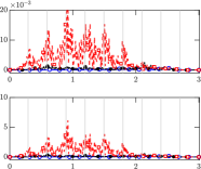
Figure 4: AS-SFD: instantaneous profiles and errors in pressure ($atm$) and velocity ($ms^{-1}$) at $t=4\times 10^{-6}s$. The different lines: blue (Set-1), black (Set-2), red (Set-3) and magenta (Set-4) are defined in Table 3. The light blue line indicates the initial condition and gray vertical lines represent processor boundaries. AS: Asynchronous with standard finite-difference schemes, S: synchronous.

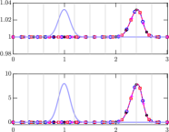
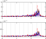
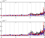
Figure 5: Asynchrony-tolerant (AT): instantaneous profiles and errors in pressure ($atm$) and velocity ($ms^{-1}$) at $t=4\times 10^{-6}s$ (left) and $t=6\times 10^{-6}s$ (right). The different lines: blue (Set-1), black (Set-2), red (Set-3) and magenta (Set-4) are defined in Table 3. The light blue line indicates the initial condition and gray vertical lines represent processor boundaries. AT: asynchronous with asynchrony-tolerant, S: synchronous.

When the standard central-difference schemes are used asynchronously (AS-SFD), there are visible fluctuations in the pressure field even at early times. This is evident from Fig. 4 where both instantaneous pressure and velocity fields at time $t=4\times 10^{-6}s$ show large numerical errors and clear deviation from the corresponding synchronous field. For larger delay values corresponding to Set-3 in Table 3, the numerical perturbations become significant at much shorter times and render the simulation unstable eventually. These errors are amplified even after the acoustic wave leaves the domain. However, when AT schemes are used for the propagation of an acoustic wave with delays at processor boundaries, the solution remains in close agreement with its synchronous counterpart and the errors are several orders of magnitude smaller (see Fig. 5). Similar behavior is also observed at later times when the wave is close to leaving the right boundary. Moreover, the errors in both pressure and velocity are not localized to near processing element boundary points where AT schemes are used to compute derivatives.

The $L_{1}$ and $L_{\infty}$ norms of the errors computed with respect to the synchronous simulation are defined as

$$Z_{L_{1}}=\langle Z_{\text{synchronous}}-Z_{\text{AS or AT}}\rangle$$ (59)

$$Z_{L_{\infty}}=\max\left(Z_{\text{synchronous}}-Z_{\text{AS or AT}}\right),$$

where $Z$ is any quantity, for example temperature, pressure or mass fractions, and $\langle.\rangle$ is the spatial average. These errors are listed in Table 5 for both AS-SFD and AT simulations at two different times. The AT schemes exhibit significantly less numerical error at both times, and the error does not grow monotonically with time like it does for the AS-SFD.

		$t=4\times 10^{-6}s$		$t=6\times 10^{-6}s$
AS-SFD
	Case	$U~{}(ms^{-1})$	$P~{}(atm)$	$U~{}(ms^{-1})$	$P~{}(atm)$
	1	3.33e-02	1.36e-04	3.30e-02	1.34e-04
$L_{1}$ error	2	9.87e-02	4.00e-04	3.78e-01	1.52e-03
	3	8.01e-01	3.26e-03	2.28e+01	9.31e-02
	1	2.27e-01	9.43e-04	2.72e-01	1.08e-03
$L_{\infty}$ error	2	6.53e-01	2.69e-03	2.03e+00	8.08e-03
	3	6.16e+00	2.57e-02	1.45e+02	7.56e-01
Asynchrony-tolerant (AT)
	Case	$U~{}(ms^{-1})$	$P~{}(atm)$	$U~{}(ms^{-1})$	$P~{}(atm)$
	1	5.88e-05	2.43e-07	3.38e-05	1.40e-07
$L_{1}$ error	2	6.70e-05	2.75e-07	4.82e-05	1.95e-07
	3	8.83e-05	3.64e-07	3.81e-05	1.57e-07
	1	5.25e-04	2.18e-06	3.27e-04	1.29e-06
$L_{\infty}$ error	2	7.84e-04	3.23e-06	4.70e-04	1.92e-06
	2	1.16e-03	4.73e-06	6.09e-04	2.56e-06

Table 5: $L_{1}$ and $L_{\infty}$ norms of error in velocity and pressure in acoustic wave propagation simulations.

5.2 Premixed Auto-ignition of $H_{2}$ using one-step chemistry

Figure 6: Temporal evolution of the peak temperature ($K$) and pressure ($atm$) during auto-ignition of a premixture of hydrogen/air in a periodic domain. The different lines (without symbols): blue (Set-1), black (Set-2), red (Set-3) and magenta (Set-4) are defined in Table 3. The dashed line indicates the time at which the instantaneous scalar and velocity profiles and errors are listed in Table 6 and Table 7.

A canonical problem of practical relevance to compression ignition in internal combustion engines is auto-ignition of a premixed fuel-air mixture at constant volume. Here auto-ignition of a fuel lean $H_{2}$/air mixture at an equivalence ratio of $0.4895$ at an initial temperature of $400K$ is considered. A hot spot represented by a Gaussian temperature spike with a peak value of $1040K$, which is above the ignition limit, is introduced at the center of a one-dimensional closed domain and the mixture eventually auto-ignites after an induction period. This thermal explosion leads to a rapid increase in temperature to nearly 2000K. Following the ignition of the hot spot, reaction fronts emanate from the spontaneous ignition kernel, one propagating to the left, while the other to the right. The gas expansion from the heat release during auto-ignition results in an induced velocity from an initially quiescent flow field. The time elapsed from the initial hot-spot to a time at which the temporal gradient of temperature or heat release rate is maximum is the so-called ignition delay time $(\tau_{ign})$. The time evolution of maximum temperature and pressure is shown in Fig. 6. It is clear that while the temperature increases slowly initially, there is an exponential increase in the temperature at around $t=5\times 10^{-5}s$. The temporal evolution of the peak temperature and pressure is captured accurately by the asynchrony-tolerant schemes. Following ignition, the two fronts propagate towards the left and right boundary and are allowed to traverse across at least one processing element boundary where delays are explicitly encountered. For simplicity we consider a periodic domain that allows us to compute spectral characteristics of both thermodynamic and hydrodynamic quantities. Note that the periodic boundary conditions considered here provide a closed volume with compression heating from the exothermic reactions that lead to a gradual rise in pressure with time. This is evident from Fig. 6 where the pressure increases from $1~{}atm$ to $1.4~{}atm$ after ignition.

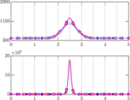
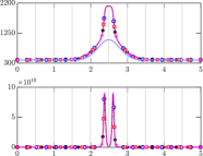
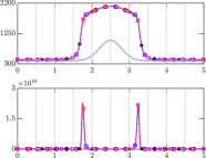
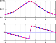
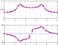
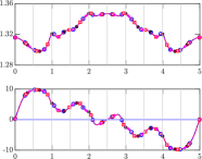
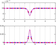
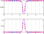
Figure 7: Asynchrony-tolerant (AT): auto-ignition of a premixed $H_{2}$/air mixture: instantaneous profiles of temperature ($K$), heat-release rate ($Jm^{-3}s^{-3}$), pressure ($atm$), velocity ($ms^{-1}$), and mass fractions of $Y_{H_{2}}$ and $Y_{H_{2}O}$. The different lines: blue (Set-1), black (Set-2), red (Set-3) and magenta (Set-4) are defined in Table 3. The light blue line indicates the initial condition and the gray vertical lines represent processor boundaries.

To investigate the effect of delays at processor boundaries on important quantities of interest both before and after spontaneous ignition, the spatial evolution of temperature, velocity, pressure, heat release, and mass fractions of hydrogen and water are shown in Fig. 7. The time instants considered are indicated with dashed-black lines in Fig. 6. Qualitatively, no difference exists between the instantaneous values of these quantities for synchronous simulation and asynchronous simulations with AT schemes. The $L_{1}$ and $L_{\infty}$ norm of error computed with respect to the synchronous simulation is listed in Table 6 and Table 7, respectively, for three time instants. Also listed are the errors when the standard schemes are used asynchronously. Note that in this case the errors are several orders of magnitude larger than AT schemes, irrespective of the quantity. Moreover, for the former case, the maximum error in temperature is approximately 9K which can trigger reactions and result in nonphysical ignition in otherwise quiescent flow due to the strong temperature dependence of reaction rates. Such numerical errors are not observed for AT schemes even when the gradients, for example, in temperature or species mass fractions exist at the processing element boundaries.

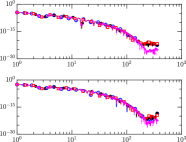
Figure 8: AS-SFD: spectra of temperature ($\hat{T}(\kappa)$), velocity ($\hat{U}(\kappa)$), and mass fractions $\hat{Y}_{H_{2}}(\kappa)$ and $\hat{Y}_{H_{2}O}(\kappa)$ for auto-ignition of a premixed $H_{2}$/air mixture. The different lines: blue (Set-1), black (Set-2), red (Set-3) and magenta (Set-4) are defined in Table 3.

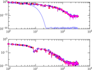
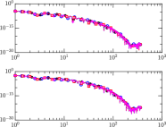
Figure 9: Asynchrony-tolerant (AT): spectra of temperature ($\hat{T}(\kappa)$), velocity ($\hat{U}(\kappa)$), and mass fractions $\hat{Y}_{H_{2}}(\kappa)$ and $\hat{Y}_{H_{2}O}(\kappa)$ for auto-ignition of premixed $H_{2}$. The different lines: blue (Set-1), black (Set-2), red (Set-3) and magenta (Set-4) are defined in Table 3.

The spectra of temperature, velocity and mass fraction of reactants and products, are shown in Fig. 8 and Fig. 9. The AT schemes exhibit excellent agreement with the synchronous simulations at all wavenumbers ($\kappa$). Moreover, non-physical accumulation of energy at high wavenumbers due to numerical errors does not exist which is in fact observed in Fig. 8 when the standard schemes are used with asynchrony. Hence, AT schemes demonstrate an excellent resolving efficiency in both physical and spectral space despite delayed data being used for the computation of derivatives at processing element boundaries.

Time	Case	$U~{}(ms^{-1})$	$P~{}(atm)$	$T~{}(K)$	$H_{2}$	$H_{2}O$
AS-SFD
	1	2.4294e-01	8.1737e-04	3.2713e-01	1.2700e-06	2.5152e-05
1.5e-4	2	3.9893e-01	1.3420e-03	5.3992e-01	2.1059e-06	4.1778e-05
	3	5.6643e-01	1.9061e-03	7.6244e-01	2.9054e-06	5.8324e-05
Asynchrony-tolerant (AT)
	1	1.07e-07	3.16e-10	8.50e-08	1.89e-13	2.29e-12
4.96e-5	2	1.23e-07	3.68e-10	8.19e-08	2.96e-13	2.31e-12
	3	1.33e-07	4.21e-10	1.11e-07	4.22e-13	3.66e-12
	1	6.80e-07	2.18e-09	7.14e-07	2.49e-12	2.53e-11
7.2e-5	2	6.46e-07	2.20e-09	9.74e-07	3.77e-12	4.89e-11
	3	1.07e-06	3.52e-09	1.09e-06	2.79e-12	3.67e-11
	1	1.17e-04	2.70e-07	7.67e-04	4.56e-09	4.87e-08
1.5e-4	2	5.67e-05	1.49e-07	2.52e-04	1.54e-09	1.61e-08
	3	1.10e-04	2.70e-07	7.17e-04	4.33e-09	4.62e-08

Table 6: $L_{1}$ norm of error in temperature, velocity, and mass fraction of $H_{2}$ and $H_{2}O$ for auto-ignition of premixed hydrogen.

Time	Case	$U~{}(ms^{-1})$	$P~{}(atm)$	$T~{}(K)$	$H_{2}$	$H_{2}O$
AS-SFD
	1	8.73e-01	2.72e-03	3.50e+00	1.80e-05	3.19e-04
1.5e-4	2	1.51e+00	4.46e-03	5.78e+00	2.96e-05	5.25e-04
	3	2.14e+00	6.23e-03	8.79e+00	4.41e-05	7.88e-04
Asynchrony-tolerant (AT)
	1	1.30e-06	2.44e-09	1.48e-06	4.61e-12	6.60e-11
2e-5	2	1.64e-06	2.30e-09	2.07e-06	1.07e-11	9.12e-11
	3	1.83e-06	2.80e-09	1.18e-06	1.19e-11	9.79e-11
	1	7.55e-06	2.64e-08	9.52e-06	7.27e-11	8.87e-10
5.52e-5	2	5.70e-06	1.95e-08	1.88e-05	1.36e-10	1.90e-09
	3	9.45e-06	3.26e-08	1.19e-05	9.30e-11	1.10e-09
	1	1.08e-03	2.44e-06	1.14e-02	5.51e-08	9.58e-07
1.5e-4	2	4.08e-04	7.97e-07	3.60e-03	1.77e-08	3.05e-07
	3	8.06e-04	1.75e-06	1.07e-02	5.12e-08	8.93e-07

Table 7: $L_{\infty}$ norm of error in temperature, velocity, and mass fraction of $H_{2}$ and $H_{2}O$ for auto-ignition of premixed hydrogen.

5.3 Auto-ignition: temperature fluctuations at the inflow boundary

The effect of turbulent fluctuations on fuel-air mixing, wrinkling of flames or spontaneous ignition front propagation is central to turbulent combustion. To simulate this effect in one-dimension and to ensure that the AT schemes can propagate fluctuations accurately across processing element boundaries, a temperature perturbation is forced at the left inflow boundary. The initial condition, shown by the light blue line in Fig. 10, is the steady state solution obtained from the auto-ignition of premixed $C_{2}H_{4}$/air mixture at a pressure of $2~{}atm$. A 22 species 18-step reduced mechanism describing the oxidation kinetics of ethylene/air [46] is used. The steady solution is perturbed with sinusoidal temperature fluctuations with a magnitude of $180K$ and frequency $20Khz$ at the left boundary using an oscillatory inflow boundary condition [47, 48]. As the perturbations approach the igniting front, the adjacent temperature increases as is evident from the increase in the mass fraction of $CH_{2}O$ radical in Fig. 10. This induces a secondary ignition kernel to the left of the initial front as can be seen in Fig. 10 (left column). The two kernels eventually interact and as time progresses, a steady ignition front develops to the left of the initial kernel as shown in the plots in the right column of Fig. 10. This front oscillates about a mean location, with the peak temperature and pressure also oscillating in response to the incoming sinusoidal fluctuations. The AT schemes accurately capture the transient and steady state evolution of both the temperature and intermediate species even in the presence of delays at the processor boundaries. An excellent qualitative agreement between the instantaneous profiles for AT and synchronous simulations in Fig. 10 is observed. Both $L_{1}$ and $L_{\infty}$ norms of the errors tabulated in Table 8 and Table 9 are also reasonably small at both times.

Time	Case	$U~{}(ms^{-1})$	$P~{}(atm)$	$T~{}(K)$	$OH$	$CH_{2}O$	$H_{2}O$
Asynchrony-tolerant (AT)
	1	3.20e-08	1.10e-10	1.32e-07	6.67e-13	3.53e-13	4.48e-12
4.48e-4	2	3.89e-08	1.27e-10	1.70e-07	8.75e-13	4.82e-13	5.91e-12
	3	4.97e-08	1.66e-10	1.75e-07	9.06e-13	4.90e-13	6.08e-12
	1	3.09e-09	1.09e-11	3.32e-08	1.50e-13	9.12e-14	1.16e-12
9.98e-4	2	3.99e-09	1.38e-11	1.93e-08	1.20e-13	4.42e-14	6.33e-13
	3	4.77e-09	1.69e-11	2.82e-08	1.69e-13	7.69e-14	8.95e-13

Table 8: Asynchrony-tolerant (AT): $L_{1}$ norm of error in temperature, velocity, and mass fraction of $OH$ and $CH_{2}O$ for auto-ignition of $C_{2}H_{4}/air$ flame with temperature fluctuations at the inflow.

Time	Case	$U~{}(ms^{-1})$	$P~{}(atm)$	$T~{}(K)$	$OH$	$CH_{2}O$	$H_{2}O$
Asynchrony-tolerant (AT)
	1	2.10e-07	8.22e-10	1.08e-06	5.76e-12	4.36e-12	5.12e-11
4.48e-4	2	2.20e-07	9.66e-10	1.53e-06	9.46e-12	6.58e-12	7.44e-11
	3	3.46e-07	1.30e-09	1.33e-06	8.23e-12	5.76e-12	6.54e-11
	1	2.05e-08	7.70e-11	5.33e-07	2.81e-12	2.15e-12	2.58e-11
1.9e-3	2	2.78e-08	1.01e-10	3.13e-07	1.68e-12	1.26e-12	1.50e-11
	3	3.57e-08	1.28e-10	4.41e-07	2.42e-12	1.83e-12	2.14e-11

Table 9: Asynchrony-tolerant (AT): $L_{\infty}$ norm of error in temperature, velocity, and mass fraction of $OH$ and $CH_{2}O$ for auto-ignition of $C_{2}H_{4}/air$ flame with temperature fluctuations at the inflow.

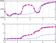
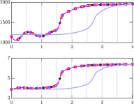
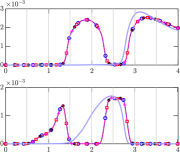
Figure 10: Asynchrony-tolerant (AT): instantaneous profiles of temperature ($K$), velocity ($ms^{-1}$), and mass fractions of $OH$ and $CH_{2}O$ radicals for autoignition of premixed $C_{2}H_{4}$/air mixtures with temperature fluctuations at the inflow. The different lines: blue (Set-1), black (Set-2), red (Set-3) and magenta (Set-4) are defined in Table 3. The light blue line indicates the initial condition and gray vertical lines represent processor boundaries.

5.4 Premixed flame propagation

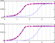
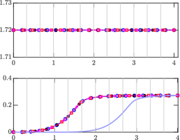
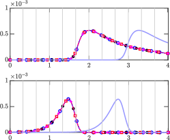
Figure 11: Asynchrony-tolerant (AT): instantaneous profiles of temperature ($K$), pressure ($atm$), velocity ($ms^{-1}$), and mass fractions of product, $H_{2}O$, and radicals, $OH$ and $CH_{2}O$, at $t=1\times 10^{-2}s$ for premixed $C_{2}H_{4}$ flame propagation. The different lines: blue (Set-1), black (Set-2), red (Set-3) and magenta (Set-4) are defined in Table 3. The light blue line indicates the initial condition and gray vertical lines represent processor boundaries.

The previous cases focused on investigation of the effect of asynchrony on spontaneous ignition dominated by unsteadiness and advection-reaction balance. The present test case is intended to study the effect of delayed data on laminar premixed flame propagation. The flame propagates at a subsonic velocity and is characterized by a balance between the reactive and diffusive terms in the steady species conservation equations. A mixture of $C_{2}H_{4}$/air at an equivalence ratio, $\phi=0.42$, $T=500~{}K$ and $P=1.72~{}atm$ is considered. The one-dimensional domain is $4~{}mm$ and is discretized with $576$ grid points that are distributed across 12 processors. The 22 species, 18-step reduced mechanism from [46] for ethylene/air used in the earlier case is also used here. The initial condition is generated using an auto-ignition case, and non-reflecting inflow and subsonic outflow are imposed at the left and right boundaries, respectively. The flame is initially located close to the right edge of the domain and in time propagates to the left while consuming the reactants mixture. The initial flame front, comprised of preheat and reaction zones, spans across three PEs as shown by the light blue line Fig. 11. This flame traverses across multiple processing element boundaries and the errors are computed to assess the effect of the asynchronous data encountered at the boundaries on flow and flame quantities.

The flame structure is invariant with time, therefore, only the instantaneous profiles and errors at the time instant when the flame approaches near the left boundary is considered for accuracy analysis. There is excellent agreement between the spatial profiles for the synchronous and the AT simulations, as shown in Fig. 11 for temperature, velocity as well as major and minor species. The drop in pressure in the reaction zone is negligibly small and thus the pressure values depicted in Fig. 11 are nearly constant. As is evident from Table 10, both $L_{1}$ and $L_{\infty}$ norms of the error between synchronous and AT simulations are negligibly small and as low as $\mathcal{O}(10^{-14})$ for some of the species. Furthermore, the flame speed computed from the time evolution of the location of the peak heat release rate is equal to $12.59~{}cm/s$ for both synchronous and asynchronous simulations. The thermal flame thickness is equal to $\delta_{T}=\frac{T_{2}-T_{1}}{\max(\partial T/\partial x)}=7.81\times 10^{-4}m$, irrespective of the delays.

Time	Case	$U~{}(ms^{-1})$	$P~{}(atm)$	$T~{}(K)$	$OH$	$CH_{2}O$	$H_{2}O$
$L_{1}$ error
	1	6.22e-11	2.32e-13	2.72e-09	2.51e-15	3.21e-15	8.60e-14
1e-2	2	9.96e-11	3.81e-13	7.12e-10	8.73e-16	8.04e-16	2.04e-14
	3	9.42e-11	3.61e-13	1.27e-09	1.16e-15	1.35e-15	3.42e-14
$L_{\infty}$ error
	1	5.72e-10	2.07e-12	1.42e-08	3.02e-14	4.66e-13	2.38e-14
1e-2	2	1.06e-09	3.07e-12	4.18e-09	8.81e-15	1.23e-13	6.31e-15
	3	6.52e-10	3.36e-12	6.61e-09	1.42e-14	2.09e-13	1.19e-14

Table 10: Asynchrony-tolerant (AT): $L_{1}$ and $L_{\infty}$ norm of error in velocity, pressure, temperature, and mass fractions of $OH$, $CH_{2}O$ and $H_{2}O$ for premixed $C_{2}H_{4}$ flame propagation.

5.5 Non-premixed ignition

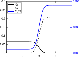
Figure 12: Initial condition for non-premixed ignition with diluted fuel on the left and vitiated air on the right.

An ignition of non-premixed $H_{2}$ using Burke’s mechanism [49] with 9 species is considered next. The setup is similar to the one used in [43] and [50] with fuel diluted with nitrogen on the left and air heated to $1500K$ on the right, as shown in Fig. 12. An inflow boundary condition from [47] is used on the left boundary with zero velocity and an outflow boundary condition is used on the right boundary with appropriate viscous conditions on each side. The one-dimensional domain is 4 $mm$ in length, discretized into 576 grid-points that are distributed across 12 PEs.

As time progresses and diffusion process tends to homogenize the gradients, there is ignition close to the stoichiometric mixture fraction, resulting in a rise in peak temperature and concentration of intermediate species. The instantaneous profiles of key quantities are shown in Fig. 13 at two times. The first series of plots on the left column in Fig. 13 are at an earlier time when ignition is localized. With time both fuel and intermediate species diffuse across processing element boundaries and the flame expands, which is shown in the plots on the right column in Fig. 13. The evolution of both major and minor species as well as temperature and velocity is accurately resolved by the AT schemes. The average and maximum errors, tabulated in Table 11 and Table 12, respectively, are both negligibly small. The errors were similarly negligible for other species that are not shown here.

Time	Case	$U~{}(ms^{-1})$	$P~{}(atm)$	$T~{}(K)$	$H_{2}$	$O$	$H$	$H_{2}O$
Asynchrony-tolerant (AT)
	1	1.94e-08	4.43e-11	1.52e-07	6.04e-12	3.63e-12	4.85e-13	2.54e-11
7.92e-5	2	2.59e-08	5.94e-11	1.97e-07	6.72e-12	5.40e-12	6.60e-13	3.74e-11
	3	3.14e-08	6.44e-11	3.13e-07	1.12e-11	7.77e-12	9.38e-13	5.42e-11
	1	5.94e-10	1.14e-12	2.57e-08	6.04e-13	2.69e-13	1.95e-14	4.43e-12
3.19e-4	2	5.25e-10	1.06e-12	3.45e-08	6.98e-13	2.55e-13	2.22e-14	5.91e-12
	3	6.18e-10	1.30e-12	5.01e-08	1.61e-12	2.56e-13	4.91e-14	4.80e-12

Table 11: Asynchrony-tolerant (AT): $L_{1}$ norm of error in temperature, velocity, and mass fractions of $H_{2}$, $O$, $H$ and $H_{2}O$ for non-premixed $H_{2}/air$ ignition.

Time	Case	$U~{}(ms^{-1})$	$P~{}(atm)$	$T~{}(K)$	$H_{2}$	$O$	$H$	$H_{2}O$
Asynchrony-tolerant (AT)
	1	1.09e-07	1.91e-10	6.10e-07	3.89e-11	1.31e-10	2.63e-11	4.05e-12
7.92e-5	2	1.11e-07	2.25e-10	8.52e-07	4.83e-11	1.85e-10	3.69e-11	5.24e-12
	3	1.21e-07	2.14e-10	1.25e-06	7.16e-11	2.73e-10	5.27e-11	7.10e-12
	1	5.08e-09	9.80e-12	9.89e-08	2.38e-12	1.65e-11	1.50e-12	7.53e-14
7.92e-5	2	4.01e-09	8.79e-12	8.94e-08	2.49e-12	1.64e-11	1.29e-12	6.47e-14
	3	4.93e-09	7.91e-12	1.52e-07	5.15e-12	1.41e-11	1.17e-12	1.38e-13

Table 12: Asynchrony-tolerant (AT): $L_{\infty}$ norm of error in temperature, velocity, and mass fractions of $H_{2}$, $O$, $H$ and $H_{2}O$ for non-premixed $H_{2}/air$ ignition.

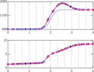
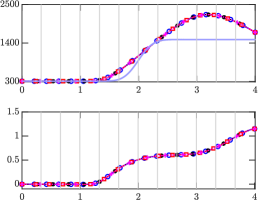
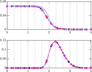
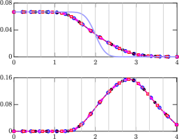
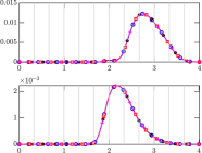
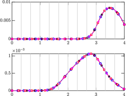
Figure 13: Asynchrony-tolerant (AT): Instantaneous profiles and error in temperature ($K$), velocity ($ms^{-1}$) and mass fractions of $H_{2}$, $H_{2}O$, $O$ and $H$ for non-premixed ignition of $H_{2}$. The different lines: blue (Set-1), black (Set-2), red (Set-3) and magenta (Set-4) are defined in Table 3. The light blue line indicates the initial condition and the gray vertical lines represent processor boundaries.

5.6 Propagation of a detonation wave

To test the numerical accuracy of AT-WENO schemes for reacting flows, a detonation of stoichiometric hydrogen/oxygen mixture diluted with argon is considered. The mixture with molar ratio $H_{2}:O_{2}:Ar=2:1:7$ is at an initial temperature of 305K and pressure of 6670 Pa. A detailed hydrogen/air mechanism [51] comprised of 9 species and 34 reversible reactions is used. A similar setup has also been used as a test case in previous studies to investigate the efficacy of numerical schemes [52, 53, 54]. A supersonic outflow condition is applied at the left boundary while a subsonic inlet condition is applied at the right boundary. The simulation is initialized with a shock that ignites the mixture at the left end of the computational domain. The domain length is $30~{}cm$ which is discretized into 6000 grid-points that are distributed across 100 PEs.

The simulation results are shown in Fig. 14 with pressure at different time instants in the leftmost plot. There is a leading shock front that compresses the fuel/air mixture followed by the induction and the reaction zones. The pressure obtained with the synchronous WENO scheme is shown in solid magenta. It is in excellent agreement with the pressure computed with the AT-WENO scheme shown in black circles and dashed lines. A zoomed-in view of the detonation structure depicted by temperature and pressure is shown in the centre plots of Fig. 14. The mixture reacts after the induction zone leading to an increase in temperature and a corresponding decrease in pressure. The mass fractions for different radicals including fuel $H_{2}$ are plotted on the rightmost plot in Fig. 14. The results of this simulation show that the detonation structure is captured accurately with the AT-WENO scheme. Furthermore, the detonation velocity obtained from standard WENO and AT-WENO simulations is $1619.7\ ms^{-1}$ and $1620.1\ ms^{-1}$, respectively. These values are in good agreement with the detonation velocity reported in previous studies [52, 53, 54]. The peak von-Neumann pressure is $165.35\ kPa$ and $165.34\ kPa$ for WENO and AT-WENO which are also similar to the previous studies. Overall, the AT-WENO schemes derived in the present study exhibit excellent numerical accuracy despite the use of delayed data at processor boundaries. Since multidimensional simulations of detonation phenomena in combustion devices face highly intensive computational resource requirements [55, 56], AT-WENO schemes hold the potential of offsetting a certain portion of communication overhead associated with standard WENO schemes at large node counts, thereby leading to improved scalability.

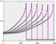
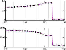
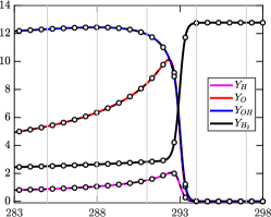
Figure 14: Asynchrony-tolerant (AT): Pressure (atm) profiles (left) at different times, structure of detonation wave (middle) for pressure (atm) and temperature ($K$) and mass fractions of $H,O,OH,H_{2}$ (right). The solid lines are standard WENO and black-dashed line with black symbols (Set-3 in Table 3) corresponds to AT-WENO. gray vertical lines represent processor boundaries.

6 Discussion

DNS of turbulent combustion at higher Reynolds numbers with detailed chemical mechanisms and at conditions relevant for practical devices will require efficient utilization of massive computing resources anticipated on next generation exascale machines. These simulations at scales and conditions that are currently infeasible will provide fine-grained details into the interactions between turbulence and chemistry and will provide fundamental insights into the physical processes that result in pollutant formation, flame stabilization, blow-off, higher efficiency, etc. This in turn will not only aid in the design of fuel-flexible, low-emission combustion engines but also in the development of physics-based models for engineering simulations that will be used to design advanced clean engines. However, a successful transition of DNS codes to exascale machines and beyond is possible only through redesign and development of new computational algorithms in order to overcome some of the obvious bottlenecks and challenges.

The anticipated computing power of a quintillion ($10^{18}$) double precision floating point operations per second on the exascale machine will be realized through extreme levels of parallelism with millions of processing elements (PEs), including CPUs, GPUs and FPGAs. For example, Frontier at the Oak Ridge Leadership Computing Facility (OCLF) will have 1:4 CPU to GPU ratio with unified memory. Despite the use of state-of-the-art low-latency, high-bandwidth communication links, the sheer number of communications will significantly hinder scaling to large node counts. To this end, efficient strategies to mask communications and data movement will be needed to improve scalability. The use of AT schemes at the PE boundaries for computation of derivatives accurately, despite delayed data, will facilitate further overlap between communications and computations. However, a challenge in extending the AT schemes to three-dimensions is that the derivatives of convective and diffusive terms need to be expanded in terms of derivatives of primitive variables by applying the chain rule. For example, $\partial(\rho ue)/\partial x:=(\rho ue)_{x}=\rho ue_{x}+\rho eu_{x}+eu\rho_{x}$. This expansion increases the total number of derivatives that need to be computed, especially when a large number of species are involved. Alternatively, one can compute the convective and diffusive terms (for example, $\rho ue,~{}\rho Y_{i}u,~{}J_{i},~{}\tau$) from the primitive variables at different time levels as required by the AT schemes. These computations can be performed on the fly in order to avoid storing such product terms at multiple time-levels. Essentially there is a trade-off between memory (data movement) and computation. Re-design of data structures for better memory coherency will also be extremely helpful since AT schemes use data from multiple time levels and can thus incur high cache miss rates. Besides these challenges, a critical first step in using AT schemes for scalable simulations of turbulent combustion on massive supercomputers is to ascertain that the numerical artifacts due to delayed data at PE boundary are significantly small and do not affect the underlying physics. The comprehensive set of numerical experiments presented in the present study specifically highlights the excellent numerical accuracy of AT schemes for compressible reacting unsteady flows.

A key component of simulations of reacting flows even for simple geometries includes the prescription of nonperiodic boundary conditions. The NSCBC [44, 45] with improvements for reacting flows [47, 48, 50, 57] has been successfully used for these simulations. In the normal direction, the terms in the NSCBC boundary conditions are not affected by AT schemes. For example, at the outflow, one-sided schemes are used, which require only local information within a PE. At the inflow, relaxation terms are used which again do not require PEs to communicate. Since transverse and viscous terms are also included for reacting flows [47, 48, 50], the AT schemes can be utilized in the transverse direction for computation of all the spatial derivatives involved. Extension to corners can be done following [57] with AT schemes used wherever necessary.

Another advantage for using asynchronous computations on exascale machines is to leverage the high flop-rate of GPUs, i.e. throughput computing. In hybrid computing architectures, GPUs are expected to handle most of the computations, while CPUs will facilitate communications between PEs. With AT schemes, GPUs will not have to wait on the CPUs for the most updated data from the neighboring PEs. This would enhance utilization of GPUs without affecting numerical accuracy or introducing idling penalties. A similar approach has been utilized in [58] where asynchronous copies between CPUs and GPUs are used to overlap computation and data movement, but delayed data with asynchronous computations have not been used. At a compiler level, new asynchronous run-time systems that are capable of dynamic task parallelism are being developed to improve the computation-communication overlap [59, 60, 61]. The AT schemes, which relax synchronization at a mathematical level, can be coupled with such data-centric programming models to create highly scalable PDE solvers. Asynchrony has also been utilized in [62] for scalable resilience to soft faults. However, in [62] all derivatives are still computed with the most updated data but the computations are re-arranged to ensure maximum overlap between communication and computation. The asynchronization approach utilized in [62] coupled with mathematical level asynchrony with AT schemes can be effective in pushing the scaling wall. Furthermore, since AT schemes do not require updated data, these schemes can also be used to recover from node failures without halting the simulation altogether.

7 Conclusions

In this paper, a series of numerical simulations that utilize delayed data at processor boundaries are presented for canonical reacting flows with single-step and detailed reaction mechanisms. It is shown that large numerical errors are incurred in physical as well as spectral space when standard schemes are used asynchronously, even for the simplest problems. To overcome this loss of accuracy, novel asynchrony-tolerant (AT) schemes are used for accurate computation of spatial derivatives with delayed data at the boundaries. These asynchronous simulations using AT schemes are compared with standard synchronous simulations and are shown to exhibit excellent qualitative and quantitative agreement. Both spatial and temporal evolution of hydrodynamic and thermo-chemical quantities are accurately captured by the AT schemes.

For simulations of high-speed flows with shocks and jump discontinuities, the standard shock-resolving WENO schemes have degraded numerical accuracy. Thus, following the procedure listed in [24] AT-WENO schemes are derived. However, the schemes so derived have non-convex linear weights which can lead to numerical instabilities and oscillations [39]. To overcome this, the asynchronous stencil is modified to include an additional grid-point. With this degree-of-freedom, an additional low-order truncation error term is selectively eliminated while preserving the convexity of the ideal weights. For evaluation of non-linear weights in AT-WENO schemes, asynchrony-tolerant smoothness indicators are also derived. The superior accuracy of AT-WENO schemes in comparison to the standard WENO schemes is exhibited through the order-of-accuracy tests for linear and non-linear equations. These schemes are also used for simulation of a detonation wave which is found to have excellent agreement with its synchronous counterpart.

A common conclusion one can arrive at through these simulations is that the AT schemes have excellent accuracy despite relaxed synchronizations at processor boundaries. Thus, AT schemes provide a potential path for highly scalable asynchronous simulations of turbulent combustion at the extreme scales promised by exascale and beyond.

Appendix A AT schemes

(Derivative,	Boundary	Scheme
Order)
(2,4)	Left	$\scriptsize\begin{array}[]{c}\frac{1}{2}({\tilde{k}}^{2}+3{\tilde{k}}+2)\left({-{u_{j+2}^{n}}+16{u_{j+1}^{n}}-30{u_{j}^{n}}+16{u_{j-1}^{n-{\tilde{k}}}}-{u_{j-2}^{n-{\tilde{k}}}}}\right)/{12\Delta x^{2}}\\ -({\tilde{k}}^{2}+2{\tilde{k}})\left({-{u_{j+2}^{n}}+16{u_{j+1}^{n}}-30{u_{j}^{n}}+16{u_{j-1}^{n-{\tilde{k}}-1}}-{u_{j-2}^{n-{\tilde{k}}-1}}}\right)/{12\Delta x^{2}}\\ +\frac{1}{2}({\tilde{k}}^{2}+{\tilde{k}})\left({-{u_{j+2}^{n}}+16{u_{j+1}^{n}}-30{u_{j}^{n}}+16{u_{j-1}^{n-{\tilde{k}}-2}}-{u_{j-2}^{n-{\tilde{k}}-2}}}\right)/{12\Delta x^{2}}\end{array}$
(2,4)	Right	$\scriptsize\begin{array}[]{c}\frac{1}{2}({\tilde{k}}^{2}+3{\tilde{k}}+2)\left({-{u_{j+2}^{n-{\tilde{k}}}}+16{u_{j+1}^{n-{\tilde{k}}}}-30{u_{j}^{n}}+16{u_{j-1}^{n}}-{u_{j-2}^{n}}}\right)/{12\Delta x^{2}}\\ -({\tilde{k}}^{2}+2{\tilde{k}})\left({-{u_{j+2}^{n-{\tilde{k}}-1}}+16{u_{j+1}^{n-{\tilde{k}}-1}}-30{u_{j}^{n}}+16{u_{j-1}^{n}}-{u_{j-2}^{n}}}\right)/{12\Delta x^{2}}\\ +\frac{1}{2}({\tilde{k}}^{2}+{\tilde{k}})\left({-{u_{j+2}^{n-{\tilde{k}}-2}}+16{u_{j+1}^{n-{\tilde{k}}-2}}-30{u_{j}^{n}}+16{u_{j-1}^{n}}-{u_{j-2}^{n}}}\right)/{12\Delta x^{2}}\end{array}$
(1,4)	Left	$\scriptsize\begin{array}[]{c}\frac{1}{2}({\tilde{k}}^{2}+3{\tilde{k}}+2)\left({-{u_{j+2}^{n}}+8{u_{j+1}^{n}}-8{u_{j-1}^{n-{\tilde{k}}}}+{u_{j-2}^{n-{\tilde{k}}}}}\right)/{12\Delta x}\\ -({\tilde{k}}^{2}+2{\tilde{k}})\left({-{u_{j+2}^{n}}+8{u_{j+1}^{n}}-8{u_{j-1}^{n-{\tilde{k}}-1}}+{u_{j-2}^{n-{\tilde{k}}-1}}}\right)/{12\Delta x}\\ +\frac{1}{2}({\tilde{k}}^{2}+{\tilde{k}})\left({-{u_{j+2}^{n}}+8{u_{j+1}^{n}}-8{u_{j-1}^{n-{\tilde{k}}-2}}+{u_{j-2}^{n-{\tilde{k}}-2}}}\right)/{12\Delta x}\end{array}$
(1,4)	Right	$\scriptsize\begin{array}[]{c}\frac{1}{2}({\tilde{k}}^{2}+3{\tilde{k}}+2)\left({-{u_{j+2}^{n-{\tilde{k}}}}+8{u_{j+1}^{n-{\tilde{k}}}}-8{u_{j-1}^{n}}+{u_{j-2}^{n}}}\right)/{12\Delta x}\\ -({\tilde{k}}^{2}+2{\tilde{k}})\left({-{u_{j+2}^{n-{\tilde{k}}-1}}+8{u_{j+1}^{n-{\tilde{k}}-1}}-8{u_{j-1}^{n}}+{u_{j-2}^{n}}}\right)/{12\Delta x}\\ +\frac{1}{2}({\tilde{k}}^{2}+{\tilde{k}})\left({-{u_{j+2}^{n-{\tilde{k}}-2}}+8{u_{j+1}^{n-{\tilde{k}}-2}}-8{u_{j-1}^{n}}+{u_{j-2}^{n}}}\right)/{12\Delta x}\end{array}$

Table 13: Asynchrony-tolerant (AT) schemes for left and right boundary used in numerical simulations for first and second derivative.

Appendix B Reconstruction approximation at the right boundary

For points located at the right processor boundary the modified smaller asynchronous stencil is given by, $\tilde{S}^{(0)}_{R}=\{u_{j-2}^{n},u_{j-1}^{n},u_{j}^{n}\}$, $\tilde{S}^{(1)}_{R}=\{u_{j-1}^{n},u_{j}^{n},u_{j}^{n-\tilde{k}},u_{j+1}^{n-\tilde{k}}u_{j+1}^{n-\tilde{k}-1}\}$, and $\tilde{S}^{(2)}_{R}=\{u_{j}^{n},u_{j+1}^{n-\tilde{k}},u_{j+1}^{n-\tilde{k}-1},u_{j+2}^{n-\tilde{k}}u_{j+2}^{n-\tilde{k}-1}\}$. Here the delay appears at the rightmost gird points. We derive the following reconstruction approximation at the right boundary,

$$\tilde{u}_{j+\frac{1}{2}}^{n,(0)}=\frac{u_{j-2}^{n}}{3}-\frac{7u_{j-1}^{n}}{6}+\frac{11u_{j}^{n}}{6}$$ (60)

$$\tilde{u}_{j+\frac{1}{2}}^{n,(1)}=-\frac{1}{3}\tilde{k}u_{j+1}^{-\tilde{k}+n-1}+\frac{1}{6}\left(2\tilde{k}+2\right)u_{j+1}^{n-\tilde{k}}-\frac{1}{6}u_{j-1}^{n}+\frac{5u_{j}^{n}}{6}$$

$$\tilde{u}_{j+\frac{1}{2}}^{n,(2)}=-\frac{5}{6}\tilde{k}u_{j+1}^{-\tilde{k}+n-1}+\frac{1}{6}\tilde{k}u_{j+2}^{-\tilde{k}+n-1}+\frac{1}{6}\left(5\tilde{k}+5\right)u_{j+1}^{n-\tilde{k}}+\frac{1}{6}\left(-\tilde{k}-1\right)u_{j+2}^{n-\tilde{k}}+\frac{u_{j}^{n}}{3}$$

Similarly, the approximation at point $u_{j-1/2}$ on the right boundary at each of the candidate stencils is listed below

$$\tilde{u}_{j-\frac{1}{2}}^{n,(0)}=-\frac{1}{6}u_{j-2}^{n}+\frac{5u_{j-1}^{n}}{6}+\frac{u_{j}^{n}}{3}$$ (61)

$$\tilde{u}_{j-\frac{1}{2}}^{n,(1)}=\frac{1}{6}\tilde{k}u_{j+1}^{-\tilde{k}+n-1}+\frac{1}{6}\left(-\tilde{k}-1\right)u_{j+1}^{n-\tilde{k}}+\frac{u_{j-1}^{n}}{3}+\frac{5u_{j}^{n}}{6}$$

$$\tilde{u}_{j-\frac{1}{2}}^{n,(2)}=\frac{7}{6}\tilde{k}u_{j+1}^{-\tilde{k}+n-1}-\frac{1}{3}\tilde{k}u_{j+2}^{-\tilde{k}+n-1}+\frac{1}{6}\left(-7\tilde{k}-7\right)u_{j+1}^{n-\tilde{k}}+\frac{1}{6}\left(2\tilde{k}+2\right)u_{j+2}^{n-\tilde{k}}+\frac{11u_{j}^{n}}{6}$$

Following the procedure described in the previous sections, the smoothness indicator at the right-boundary can be computed to be

$$\tilde{\beta}^{(0)}=\frac{1}{3} \Bigg{(}4\left(u^{n}\right)_{j-2}^{2}+\left(11u^{n}_{j}-19u^{n}_{j-1}\right)u^{n}_{j-2}+25\left(u^{n}\right)_{j-1}^{2}+10\left(u^{n}\right)_{j}^{2}-31u^{n}_{j-1}u^{n}_{j}\Bigg{)}$$ (62)

$$\tilde{\beta}^{(1)}=\frac{1}{3} \Bigg{(}u_{j-1}^{n}\left(-5\tilde{k}u_{j+1}^{n-\tilde{k}-1}+5\left(\tilde{k}+1\right)u_{j+1}^{n-\tilde{k}}-13u_{j}^{n}\right)+4\left(\tilde{k}u_{j+1}^{n-\tilde{k}-1}-\left(\tilde{k}+1\right)u_{j+1}^{n-\tilde{k}}\right)^{2}$$ (63)

$$+13u_{j}^{n}\Big{(}\tilde{k}u_{j+1}^{n-\tilde{k}-1}-\left(\tilde{k}+1\right)u_{j+1}^{n-\tilde{k}}\Big{)}+4\left(u_{j-1}^{n}\right)^{2}+13\left(u_{j}^{n}\right)^{2}\Bigg{)}$$

$$\tilde{\beta}^{(2)}=\frac{1}{3} \Bigg{(}\tilde{k}^{2}\Bigg{(}25\left(u_{j+1}^{n-\tilde{k}-1}\right)^{2}+\left(19\left(u_{j+2}^{n-\tilde{k}}-u_{j+2}^{n-\tilde{k}-1}\right)-50u_{j+1}^{n-\tilde{k}}\right)u_{j+1}^{n-\tilde{k}-1}+25\left(u_{j+1}^{n-\tilde{k}}\right)^{2}$$ (64)

$$+4\left(u_{j+2}^{n-\tilde{k}-1}-u_{j+2}^{n-\tilde{k}}\right)^{2}+19u_{j+1}^{n-\tilde{k}}\left(u_{j+2}^{n-\tilde{k}-1}-u_{j+2}^{n-\tilde{k}}\right)\Bigg{)}+\tilde{k}\Big{(}50\left(u_{j+1}^{n-\tilde{k}}\right)^{2}$$

$$+19\left(u_{j+2}^{n-\tilde{k}-1}-2u_{j+2}^{n-\tilde{k}}\right)u_{j+1}^{n-\tilde{k}}+8u_{j+2}^{n-\tilde{k}}\left(u_{j+2}^{n-\tilde{k}}-u_{j+2}^{n-\tilde{k}-1}\right)+u_{j+1}^{n-\tilde{k}-1}\left(19u_{j+2}^{n-\tilde{k}}-50u_{j+1}^{n-\tilde{k}}\right)\Big{)}$$

$$+25\left(u_{j+1}^{n-\tilde{k}}\right)^{2}+4\left(u_{j+2}^{n-\tilde{k}}\right)^{2}-19u_{j+1}^{n-\tilde{k}}u_{j+2}^{n-\tilde{k}}+u_{j}^{n}\Big{(}-31u_{j+1}^{n-\tilde{k}}+11u_{j+2}^{n-\tilde{k}}$$

$$+\tilde{k}\left(31u_{j+1}^{n-\tilde{k}-1}-31u_{j+1}^{n-\tilde{k}}-11u_{j+2}^{n-\tilde{k}-1}+11u_{j+2}^{n-\tilde{k}}\right)\Big{)}+10\left(u_{j}^{n}\right)^{2}\Bigg{)}$$

Lastly, we note that the approximation of $u_{j-1/2}$ at the left-boundary is

$$\tilde{u}_{j-\frac{1}{2}}^{n,(0)}=\frac{1}{6}\tilde{k}u_{j-2}^{-\tilde{k}+n-1}-\frac{5}{6}\tilde{k}u_{j-1}^{-\tilde{k}+n-1}+\frac{1}{6}\left(-\tilde{k}-1\right)u_{j-2}^{n-\tilde{k}}+\frac{1}{6}\left(5\tilde{k}+5\right)u_{j-1}^{n-\tilde{k}}+\frac{u_{j}^{n}}{3}$$ (65)

$$\tilde{u}_{j-\frac{1}{2}}^{n,(1)}=-\frac{1}{3}\tilde{k}u_{j-1}^{-\tilde{k}+n-1}+\frac{1}{6}\left(2\tilde{k}+2\right)u_{j-1}^{n-\tilde{k}}+\frac{5u_{j}^{n}}{6}-\frac{u_{j+1}^{n}}{6}$$

$$\tilde{u}_{j-\frac{1}{2}}^{n,(2)}=\frac{11}{6}{u_{j}^{n}}-\frac{7}{6}u_{j+1}^{n}+\frac{1}{3}u_{j+2}^{n}.$$

References

- Moin and Mahesh [1998] P. Moin, K. Mahesh, DIRECT NUMERICAL SIMULATION: A Tool in Turbulence Research, Annu. Rev. Fluid Mech. 30 (1998) 539–578.
- Visbal et al. [2001] M. Visbal, D. Gaitonde, D. Rizzetta, High-order schemes for DNS/LES and CAA on curvilinear dynamic meshes, DNS/LES Progress and Challenges, Greyden Press (2001).
- Chen et al. [2009] J. H. Chen, A. Choudhary, B. de Supinski, M. DeVries, E. R. Hawkes, S. Klasky, W. K. Liao, K. L. Ma, J. Mellor-Crummey, N. Podhorszki, R. Sankaran, S. Shende, C. S. Yoo, Terascale direct numerical simulations of turbulent combustion using S3D, Comput. Sci. Disc. 2 (2009) 015001.
- Attili et al. [2014] A. Attili, F. Bisetti, M. E. Mueller, H. Pitsch, Formation, growth, and transport of soot in a three-dimensional turbulent non-premixed jet flame, Combustion and Flame 161 (2014) 1849–1865.
- Aditya et al. [2019] K. Aditya, A. Gruber, C. Xu, T. Lu, A. Krisman, M. R. Bothien, J. H. Chen, Direct numerical simulation of flame stabilization assisted by autoignition in a reheat gas turbine combustor, Proceedings of the Combustion Institute 37 (2019) 2635–2642.
- Savard et al. [2019] B. Savard, E. R. Hawkes, K. Aditya, H. Wang, J. H. Chen, Regimes of premixed turbulent spontaneous ignition and deflagration under gas-turbine reheat combustion conditions, Combustion and Flame 208 (2019) 402–419.
- Gruber et al. [2018] A. Gruber, E. S. Richardson, K. Aditya, J. H. Chen, Direct numerical simulations of premixed and stratified flame propagation in turbulent channel flow, Phys. Rev. Fluids 3 (2018) 110507.
- Zhang et al. [2021] J. Zhang, M. B. Luong, F. E. H. Pérez, D. Han, H. G. Im, Z. Huang, Exergy loss characteristics of DME/air and ethanol/air mixtures with temperature and concentration fluctuations under HCCI/SCCI conditions: A DNS study, Combustion and Flame 226 (2021) 334–346.
- Berger et al. [2020] L. Berger, R. Hesse, K. Kleinheinz, M. J. Hegetschweiler, A. Attili, J. Beeckmann, G. T. Linteris, H. Pitsch, A DNS study of the impact of gravity on spherically expanding laminar premixed flames, Combustion and Flame 216 (2020) 412–425.
- Kim et al. [2021] Y. J. Kim, B. J. Lee, H. G. Im, Effects of Differential Diffusion on the Stabilization of Unsteady Lean Premixed Flames Behind a Bluff-Body, Flow Turbulence Combust (2021) 1125– 1141.
- Nivarti and Cant [2017] G. Nivarti, S. Cant, Direct numerical simulation of the bending effect in turbulent premixed flames, Proceedings of the Combustion Institute 36 (2017) 1903–1910.
- Desai et al. [2021] S. Desai, Y. J. Kim, W. Song, M. B. Luong, F. E. H. Pérez, R. Sankaran, H. G. Im, Direct numerical simulations of turbulent reacting flows with shock waves and stiff chemistry using many-core/gpu acceleration, Computers & Fluids 215 (2021) 104787.
- Beardsell and Blanquart [2021] G. Beardsell, G. Blanquart, Fully compressible simulations of the impact of acoustic waves on the dynamics of laminar premixed flames for engine-relevant conditions, Proceedings of the Combustion Institute 38 (2021) 1923–1931.
- Aditya and Donzis [2012] K. Aditya, D. A. Donzis, Poster: Asynchronous computing for partial differential equations at extreme scales, in: Proceedings of the 2012 SC Companion: High Performance Computing, Networking Storage and Analysis, SCC ’12, IEEE Computer Society, Washington, DC, USA, 2012, p. 1444.
- Donzis and Aditya [2014] D. A. Donzis, K. Aditya, Asynchronous finite-difference schemes for partial differential equations, J. Comp. Phys. 274 (2014) 370–392.
- Dongarra et al. [2011] J. Dongarra, P. Beckman, T. Moore, P. Aerts, G. Aloisio, J.-C. Andre, D. Barkai, J.-Y. Berthou, T. Boku, B. Braunschweig, F. Cappello, B. Chapman, Xuebin Chi, A. Choudhary, S. Dosanjh, T. Dunning, S. Fiore, A. Geist, B. Gropp, R. Harrison, M. Hereld, M. Heroux, A. Hoisie, K. Hotta, Zhong Jin, Y. Ishikawa, F. Johnson, S. Kale, R. Kenway, D. Keyes, B. Kramer, J. Labarta, A. Lichnewsky, T. Lippert, B. Lucas, B. Maccabe, S. Matsuoka, P. Messina, P. Michielse, B. Mohr, M. S. Mueller, W. E. Nagel, H. Nakashima, M. E. Papka, D. Reed, M. Sato, E. Seidel, J. Shalf, D. Skinner, M. Snir, T. Sterling, R. Stevens, F. Streitz, B. Sugar, S. Sumimoto, W. Tang, J. Taylor, R. Thakur, A. Trefethen, M. Valero, A. van der Steen, J. Vetter, P. Williams, R. Wisniewski, K. Yelick, The International Exascale Software Project roadmap, The International Journal of High Performance Computing Applications 25 (2011) 3–60.
- Bertsekas and Tsitsiklis [1989] D. P. Bertsekas, J. N. Tsitsiklis, Parallel and Distributed Computation: Numerical Methods, Prentice-Hall, Inc., USA, 1989.
- Frommer and Szyld [2000] A. Frommer, D. B. Szyld, On asynchronous iterations, Journal of Computational and Applied Mathematics 123 (2000) 201–216.
- Lee et al. [2016] K. Lee, R. Bhattacharya, J. Dass, V. N. S. P. Sakuru, R. N. Mahapatra, A Relaxed Synchronization Approach for Solving Parallel Quadratic Programming Problems with Guaranteed Convergence, in: 2016 IEEE International Parallel and Distributed Processing Symposium (IPDPS), pp. 182–191.
- Lee et al. [2015] K. Lee, R. Bhattacharya, V. Gupta, A switched dynamical system framework for analysis of massively parallel asynchronous numerical algorithms, in: 2015 American Control Conference (ACC), pp. 1095–1100.
- Amitai et al. [1992] D. Amitai, A. Averbuch, S. Itzikowitz, M. Israeli, Parallel adaptive and time-stabilizing schemes for constant-coefficient parabolic pde’s, Computers & Mathematics with Applications 24 (1992) 33 – 53.
- Amitai et al. [1994] D. Amitai, A. Averbuch, S. Itzikowitz, E. Turkel, Asynchronous and corrected-asynchronous finite difference solutions of PDEs on MIMD multiprocessors, Numer. Algorithms 6 (1994) 275–296.
- Mittal and Girimaji [2017] A. Mittal, S. Girimaji, Proxy-equation paradigm: A strategy for massively parallel asynchronous computations, Phys. Rev. E 96 (2017) 033304.
- Aditya and Donzis [2017] K. Aditya, D. A. Donzis, High-order asynchrony-tolerant finite difference schemes for partial differential equations, Journal of Computational Physics 350 (2017) 550–572.
- Mudigere et al. [2014] D. Mudigere, S. D. Sherlekar, S. Ansumali, Delayed Difference Scheme for Large Scale Scientific Simulations, Phys. Rev. Lett. 113 (2014) 218701.
- Aditya et al. [2019] K. Aditya, T. Gysi, G. Kwasniewski, T. Hoefler, D. A. Donzis, J. H. Chen, A scalable weakly-synchronous algorithm for solving partial differential equations, 2019.
- Kumari and Donzis [2020] K. Kumari, D. A. Donzis, Direct numerical simulations of turbulent flows using high-order asynchrony-tolerant schemes: Accuracy and performance, Journal of Computational Physics 419 (2020) 109626.
- Kumari and Donzis [2021] K. Kumari, D. A. Donzis, A generalized von Neumann analysis for multi-level schemes: Stability and spectral accuracy, Journal of Computational Physics 424 (2021) 109868.
- Hoefler et al. [2010] T. Hoefler, T. Schneider, A. Lumsdaine, Characterizing the Influence of System Noise on Large-Scale Applications by Simulation, in: International Conference for High Performance Computing, Networking, Storage and Analysis (SC’10).
- Shu [1998] C.-W. Shu, Essentially non-oscillatory and weighted essentially non-oscillatory schemes for hyperbolic conservation laws, in: A. Quarteroni (Ed.), Advanced Numerical Approximation of Nonlinear Hyperbolic Equations: Lectures given at the 2nd Session of the Centro Internazionale Matematico Estivo (C.I.M.E.) Held in Cetraro, Italy, June 23–28, 1997, Springer Berlin Heidelberg, Berlin, Heidelberg, 1998, pp. 325–432.
- Shu [2009] C.-W. Shu, High Order Weighted Essentially Nonoscillatory Schemes for Convection Dominated Problems, SIAM Rev. 51 (2009) 82–126.
- Pirozzoli [2011] S. Pirozzoli, Numerical methods for high-speed flows, Annual review of fluid mechanics 43 (2011) 163–194.
- Bermejo-Moreno et al. [2013] I. Bermejo-Moreno, J. Bodart, J. Larsson, B. M. Barney, J. W. Nichols, S. Jones, Solving the compressible navier-stokes equations on up to 1.97 million cores and 4.1 trillion grid points, in: SC ’13: Proceedings of the International Conference on High Performance Computing, Networking, Storage and Analysis, pp. 1–10.
- Mosedale and Drikakis [2007] A. Mosedale, D. Drikakis, Assessment of Very High Order of Accuracy in Implicit LES models, Journal of Fluids Engineering 129 (2007) 1497–1503.
- Ritos et al. [2018a] K. Ritos, I. W. Kokkinakis, D. Drikakis, Physical insight into the accuracy of finely-resolved iLES in turbulent boundary layers, Computers & Fluids 169 (2018a) 309–316.
- Ritos et al. [2018b] K. Ritos, I. W. Kokkinakis, D. Drikakis, Performance of high-order implicit large eddy simulations, Computers & Fluids 173 (2018b) 307–312.
- Shu [2020] C.-W. Shu, Essentially non-oscillatory and weighted essentially non-oscillatory schemes, Acta Numerica (2020) 63.
- Jiang and Shu [1996] G.-S. Jiang, C.-W. Shu, Efficient implementation of weighted eno schemes, Journal of Computational Physics 126 (1996) 202–228.
- Shi et al. [2002] J. Shi, C. Hu, C.-W. Shu, A Technique of Treating Negative Weights in WENO Schemes, Journal of Computational Physics 175 (2002) 108–127.
- Liu et al. [2009] Y.-y. Liu, C.-w. Shu, M.-p. Zhang, On the positivity of linear weights in weno approximations, Acta Mathematicae Applicatae Sinica, English Series 25 (2009) 503–538.
- Kee et al. [1996] R. J. Kee, F. M. Rupley, E. Meeks, J. A. Miller, CHEMKIN-III: A FORTRAN chemical kinetics package for the analysis of gas-phase chemical and plasma kinetics, Technical Report, Sandia National Labs., Livermore, CA (United States), 1996.
- Kee et al. [1986] R. J. Kee, G. Dixon-Lewis, J. Warnatz, M. E. Coltrin, J. A. Miller, A fortran computer code package for the evaluation of gas-phase multicomponent transport properties, Sandia National Laboratories Report SAND86-8246 13 (1986) 80401–1887.
- Baum et al. [1995] M. Baum, T. Poinsot, D. Thévenin, Accurate boundary conditions for multicomponent reactive flows, Journal of Computational Physics 116 (1995) 247 – 261.
- Thompson [1987] K. W. Thompson, Time dependent boundary conditions for hyperbolic systems, Journal of Computational Physics 68 (1987) 1–24.
- Poinsot and Lele [1992] T. J. Poinsot, S. K. Lele, Boundary conditions for direct simulations of compressible viscous flows, Journal of Computational Physics 101 (1992) 104–129.
- Luo et al. [2012] Z. Luo, C. S. Yoo, E. S. Richardson, J. H. Chen, C. K. Law, T. Lu, Chemical explosive mode analysis for a turbulent lifted ethylene jet flame in highly-heated coflow, Combustion and Flame 159 (2012) 265–274.
- Yoo et al. [2005] C. S. Yoo, Y. Wang, A. Trouvé, H. G. Im, Characteristic boundary conditions for direct simulations of turbulent counterflow flames, Combustion Theory and Modelling 9 (2005) 617–646.
- Yoo and Im [2007] C. S. Yoo, H. G. Im, Characteristic boundary conditions for simulations of compressible reacting flows with multi-dimensional, viscous and reaction effects, Combustion Theory and Modelling 11 (2007) 259–286.
- Burke et al. [2012] M. P. Burke, M. Chaos, Y. Ju, F. L. Dryer, S. J. Klippenstein, Comprehensive h2/o2 kinetic model for high-pressure combustion, International Journal of Chemical Kinetics 44 (2012) 444–474.
- Sutherland and Kennedy [2003] J. C. Sutherland, C. A. Kennedy, Improved boundary conditions for viscous, reacting, compressible flows, Journal of Computational Physics 191 (2003) 502–524.
- Westbrook [1982] C. K. Westbrook, Chemical kinetics of hydrocarbon oxidation in gaseous detonations, Combustion and Flame 46 (1982) 191 – 210.
- Deiterding [2003] R. Deiterding, Parallel adaptive simulation of multi-dimensional detonation structures (2003).
- Lv and Ihme [2014] Y. Lv, M. Ihme, Discontinuous Galerkin method for multicomponent chemically reacting flows and combustion, Journal of Computational Physics 270 (2014) 105–137.
- Houim and Kuo [2011] R. W. Houim, K. K. Kuo, A low-dissipation and time-accurate method for compressible multi-component flow with variable specific heat ratios, Journal of Computational Physics 230 (2011) 8527–8553.
- Luong et al. [2020a] M. B. Luong, S. Desai, F. E. H. Pérez, R. Sankaran, B. Johansson, H. G. Im, A statistical analysis of developing knock intensity in a mixture with temperature inhomogeneities, Proceedings of the Combustion Institute (2020a).
- Luong et al. [2020b] M. B. Luong, S. Desai, F. E. Hernández Pérez, R. Sankaran, B. Johansson, H. G. Im, Effects of turbulence and temperature fluctuations on knock development in an ethanol/air mixture, Flow, Turbulence and Combustion (2020b) 1–21.
- Lodato and Pitsch [2011] G. Lodato, H. Pitsch, Characteristic outflows with optimal transverse terms: The edges and corners coupling algorithm, Center for Turbulence Research, Annual Research Briefs (2011) 12.
- Yeung and Ravikumar [2020] P. K. Yeung, K. Ravikumar, Advancing understanding of turbulence through extreme-scale computation: Intermittency and simulations at large problem sizes, Phys. Rev. Fluids 5 (2020) 110517.
- Slaughter et al. [2015] E. Slaughter, W. Lee, S. Treichler, M. Bauer, A. Aiken, Regent: A high-productivity programming language for hpc with logical regions, in: Proceedings of the International Conference for High Performance Computing, Networking, Storage and Analysis, SC ’15, Association for Computing Machinery, New York, NY, USA, 2015.
- Acun et al. [2014] B. Acun, A. Gupta, N. Jain, A. Langer, H. Menon, E. Mikida, X. Ni, M. Robson, Y. Sun, E. Totoni, L. Wesolowski, L. Kale, Parallel programming with migratable objects: Charm++ in practice, in: SC ’14: Proceedings of the International Conference for High Performance Computing, Networking, Storage and Analysis, pp. 647–658.
- Kulkarni and Lumsdaine [2019] A. Kulkarni, A. Lumsdaine, A comparative study of asynchronous many-tasking runtimes: Cilk, charm++, parallex and am++, arXiv preprint arXiv:1904.00518 (2019).
- Kolla et al. [2020] H. Kolla, J. R. Mayo, K. Teranishi, R. C. Armstrong, Improving scalability of silent-error resilience for message-passing solvers via local recovery and asynchrony, 2020 IEEE/ACM 10th Workshop on Fault Tolerance for HPC at eXtreme Scale (FTXS) (2020) 1–10.