Masses and Thermodynamic Quantities of Quarkonia in Nonrelativistic Quark Model

Abstract

The temperature dependent energy, mass and some of thermodynamic quantities of charmonium and bottomonium have been calculated by solving the radial Schrödinger equation with the extended Cornell potential at finite temperature using the Nikiforov-Uvarov method. Obtained results accord with experimental data and theoretical results of the previous studies. We have found the spectrum of quarkonia mass strictly decreases at high values of temperature.

Keywords: Schrödinger equation; Nikiforov-Uvarov method; Quarkonia; Charmonium; Bottomonium

Introduction

Heavier mesons also known as quarkonia are constituents of heavy quarks such as the charmed (c) and bottom(b). The study of the system of the heavy quarkonium plays a very important role for the Standard Model (SM) and also for the quantifiable test of Quantum Chromodynamics (QCD). It is a topic of interest for the high energy physics [1, 2, 3, 4, 5, 6]. The quarkonia plays an important role in obtaining information on the restoration of spontaneously broken chiral symmetry in a nuclear medium and understanding quark gluon plasma as a new phase of hadronic matter. It was believed that the quarkonia can help us to extract the nature of quark-antiquark interaction at the hadronic scale and play the same role in probing the QCD as the hydrogen atom plan in the atomic physics.

QCD have played an important role in understanding quarkonium spectroscopy since the discovery of charmonium states.There are several equations for quarkonium corresponding to various assumptions, each derived in different theoretical framework. The initial models describing charmonium spectroscopy, using a QCD motivated Coulomb plus linear confining potential with color magnetic spin dependent interactions have successfully been used. This approach provides a useful framework for refining our understanding of QCD and also is a guide toward progress in quarkonium physics. Also, all of the open quantum system approaches to quarkonium dynamics have examined in the quark-gluon plasma. The Cornell potential and its extended forms have been successful in describing most known mesons. In the nonrelativistic quantum mechanic, quarkonia is a bound system and it is described by two particle Schrödinger equation. The radial Schrödinger equation can be solved by the real part of complex value potential and the solution can be used to understand different phenomena in the study of the atomic physics, nuclear physics and also in high energy physics, which are not yet understood [7]. The radial Schrödinger equation has been solved by using different methods [8, 9, 10, 11, 12].

One of the methods used in the analytical solution of the Schrödinger equation is the Nikiforov-Uvanov method [13]. This method has been introduced for the solution of the Schrödinger equation to its energy levels by transforming it into hyper-geometric type seconder differential equations. It is based on the determination of the wave function solution in terms of special orthogonal functions for any general second order differential equation. Alberico et. al. [14], Moscy et. al.[15] Agotiya et. al.[7] Abu-Shady et.al.[16] and Ahmadov et.al.[17, 18, 19, 20] have solved the Schrödinger equation at finite temperature by using a temperature dependent effective potential.

The study of thermodynamics quantities for quantum systems in different potential has received special attention in the last decades [21, 22, 23, 24]. For a deep understanding of the thermal effects on various physical systems, the energy behavior of the Schrödinger equation for a particle in a gas system with an interaction potential and also the features of particle with respect to thermodynamic properties has to be investigated. Recently, many authors have studied the thermodynamic properties of particle systems. There are a large number of potentials used in Schrödinger, Klein-Gordon or Dirac equations [25, 26] with physical importance.

In this study, we consider the extended Cornell potential and calculate the temperature dependent energy, mass and thermodynamic quantities (free energy $F(\beta)$, mean energy $U(\beta)$, specific heat $C(\beta)$, entropy $\mathcal{S}(\beta)$ and magnetic susceptibility $\chi(\beta)$ in terms of canonical partition function $Z(\beta)$) for quarkonia. In contrast to the previous studies using fixed temperature ($T=0$)for the mass calculations, we calculated mass at varying temperatures.

The rest of the paper is structured as follows: In Section 2, we present the calculations of the temperature dependent energy eigenvalue expansion and quarkonium mass, calculations of the thermodynamic quantities are given in Section 3. The numerical results and our discussion is provided in Section 4. Finally Section 5. is reserved for the conclusion.

Temperature Dependent Radial Schrödinger Equation and Quarkonia Masses

The radial Schrödinger equation for two particles ($c=1$ and $\not{h}=1$) interacting via a potential in the three dimensional space is given in [19] as:

$$\chi^{\prime\prime}(r)+2\mu\left[E-{1\over 2\mu}{L(L+1)\over r^{2}}-V(r)\right]\chi(r)=0$$ (1)

where $\mu$ and $L$ are the reduce mass for the quarkonium particle and the angular momentum quantum number, respectively.

We consider the extended Cornell potential, which is the sum of the Cornell potential, the inverse quadratic potential and the harmonic potential.

Our choice for the radial scalar power potential is

$$V(r)=Ar-\frac{B}{r}+\frac{C}{r^{2}}+Dr^{2}.$$ (2)

Based on the success of the potential of the model at zero temperature, and on the idea that color screening implies modification of the inter-quark forces, potential models have been used to try to understand quarkonia properties at finite temperature [15]. In a thermodynamics environment of interacting quarks and gluons, at temperature $T$, quark binding becomes modified by color screening. Following the same philosophy for Cornell potential in [7, 27, 28, 29, 30] and making the potential term as temperature dependent as follows

$$V(r,T)=\mathcal{A}(r,T)r-\frac{\mathcal{B}(r,T)}{r}+\frac{\mathcal{C}(r,T)}{r^{2}}+\mathcal{D}(r,T)r^{2}$$ (3)

where

$$\mathcal{A}(r,T)=\frac{A}{m_{D}(T)r}\left(1-e^{-m_{D}(T)r}\right)\quad,\quad\mathcal{B}(r,T)=Be^{-m_{D}(T)r}$$

$$\mathcal{C}(r,T)=Ce^{-m_{D}(T)r}\quad,\quad\mathcal{D}(r,T)=\frac{D}{m_{D}(T)r}\left(1-e^{-m_{D}(T)r}\right)$$

such that $m_{D}(T)=\gamma\alpha_{s}(T)T$ is the Debye screening mass which vanishes as $T=0$ and $\alpha_{s}(T)$ is the running coupling constant $\alpha_{s}(T)=\frac{2\pi}{(11-{2\over 3}N_{f})\ln(T/\Lambda)}$ [31, 32, 33, 34, 35, 36]. Using the approximation $e^{-m_{D}(T)r}\approx 1-m_{D}(T)r+\frac{1}{2}m_{D}^{2}(T)r^{2}$ up to second order which give a good accuracy for $m_{D}(T)r\ll 1$. Then we obtain

$$\begin{array}[]{rcl}V(r,T)&=&\displaystyle Bm_{D}(T)+\frac{1}{2}Cm_{D}^{2}(T)+\left(A-\frac{1}{2}Bm_{D}^{2}(T)\right)r-\left(B+Cm_{D}^{2}(T)\right)\frac{1}{r}\\ &+&\displaystyle\left(D-\frac{1}{2}Am_{D}(T)\right)r^{2}+\frac{C}{r^{2}}-\frac{1}{2}Dm_{D}(T)r^{3}\\ &=&\displaystyle F+Gr-\frac{K}{r}+Mr^{2}+\frac{C}{r^{2}}-Nr^{3}.\par\end{array}$$ (4)

If we substitute the value of $V(r,T)$ in Eq(1) we get

$$\chi^{\prime\prime}(r)+2\mu\left[E-\frac{\hbar^{2}}{2}\frac{L(L+1)}{\mu r^{2}}-F-Gr+\frac{K}{r}-Mr^{2}-\frac{C}{r^{2}}+Nr^{3}\right]\chi(r)=0.$$ (5)

Using $\displaystyle r=\frac{1}{x}$ Eq.(5) becomes:

$$\chi^{\prime\prime}(x)+\frac{2x}{x^{2}}\chi^{\prime}(x)+2\mu\frac{1}{x^{4}}\left[E-\frac{\hbar^{2}}{2\mu}L(L+1)x^{2}-F-\frac{G}{x}+Kx-\frac{M}{x^{2}}-Cx^{2}+\frac{N}{x^{3}}\right]\chi(x)=0.$$ (6)

Let us consider a characteristic radius of quark and antiquark system, which is the minimum interval between two quark at which they cannot collide with each other. Setting $y=x-\delta$, we expand the terms $\frac{G}{x},\frac{M}{x^{2}}$ and $\frac{N}{x^{3}}$ in powers series form around $r_{0}\left(\delta=\frac{1}{r_{0}}\right)$ using up to the second-order terms only, we obtain:

$$\frac{G}{x}=G\left(\frac{3}{\delta}-\frac{3x}{\delta^{2}}+\frac{x}{\delta^{3}}\right)$$ (7)

$$\frac{M}{x^{2}}=M\left(\frac{6}{\delta^{2}}-\frac{8x}{\delta^{3}}+\frac{3x^{2}}{\delta^{4}}\right)$$ (8)

$$\frac{N}{x^{3}}=N\left(\frac{10}{\delta^{3}}-\frac{15x}{\delta^{4}}+\frac{6x^{2}}{\delta^{5}}\right).$$ (9)

This approximation is similar to Pekeris approximation [37, 38] that causes deformation of the centrifugal potential.

By substituting Eqs.(7-9) into Eq.(6):

$$\begin{array}[]{rcl}\displaystyle\chi^{\prime\prime}(x)+\frac{2x}{x^{2}}\chi^{\prime}(x)&+&\displaystyle 2\mu\frac{1}{x^{4}}\left[\left(E-F-\frac{3G}{\delta}+\frac{3M}{\delta^{2}}+\frac{10N}{\delta^{3}}\right)+\left(K-\frac{3G}{\delta^{2}}-\frac{8M}{\delta^{3}}-\frac{15N}{\delta^{4}}\right)x\right.\\ &+&\displaystyle\left.\left(-\frac{1}{2\mu}L(L+1)-C-\frac{G}{\delta^{3}}+\frac{3M}{\delta^{4}}+\frac{6N}{\delta^{5}}\right)x^{2}\right]\chi(x)=0.\end{array}$$ (10)

Now, we have the second-order differential equation

$$\chi^{\prime\prime}(x)+\frac{\widetilde{\tau}(x)}{\sigma(x)}\chi^{\prime}(x)+\frac{\widetilde{\sigma}(x)}{\sigma^{2}(x)}\chi(x)=0$$ (11)

where $\widetilde{\tau}(x)=2x,\sigma(x)=x^{2}$ and $\tilde{\sigma}(x)=2\mu\left(-D_{1}+D_{2}x-D_{3}x^{2}\right)$ such that $\sigma(x)$ and $\tilde{\sigma}(x)$ are polynomials of degree not greater than two and $\widetilde{\tau}(x)$ is a polynomial of degree not greater than one.

Then, we can use the Nikiforov-Uvarov (NU) method for the solution of the above equation. Following similar approaches in in [18, 19, 20] we obtain the temperature dependent energy eigenvalue expansion as:

$$\begin{array}[]{rcl}\displaystyle E_{nl}&=&\displaystyle a_{1}+a_{2}m_{D}(T)+a_{3}m_{D}^{2}(T)\\ \displaystyle\hfil&-&\displaystyle 2\mu\left[\frac{b_{1}+b_{2}m_{D}(T)+b_{3}m_{D}^{2}(T)}{2n+1+\sqrt{1+4L(L+1)+c_{1}+c_{2}m_{D}(T)+c_{3}m_{D}^{2}(T)}}\right]^{2}\end{array}$$ (12)

where

$$a_{1}=\frac{3A}{\delta}+\frac{6D}{\delta^{2}}\quad,\quad a_{2}=B-\frac{3A}{\delta^{2}}-\frac{5D}{\delta^{3}}\quad,\quad a_{3}=\frac{1}{2}C-\frac{3B}{2\delta^{2}}$$

$$b_{1}=B+\frac{3A}{\delta^{2}}+\frac{8D}{\delta^{3}}\quad,\quad b_{2}=C-\frac{4A}{\delta^{3}}-\frac{15D}{2\delta^{4}}\quad,\quad b_{3}=-\frac{3B}{2\delta^{2}}$$

$$c_{1}=8\mu\left(C+\frac{A}{\delta^{3}}+\frac{3D}{\delta^{4}}\right)\quad,\quad c_{2}=-8\mu\left(\frac{3A}{\delta^{4}}-\frac{3D}{\delta^{5}}\right)\quad,\quad c_{3}=-8\mu\frac{B}{2\delta^{4}}.$$

We would like to note that the results of Eqn. (12) are same as given for $N=3$ in [16] and for $T=0$ in [16, 20].

In general, the quark and anti-quark bound states are represented by ${}_{n}^{2s+1}L_{j}$ identified with the $J^{PC}$ values with $\overrightarrow{J}=\overrightarrow{L}+\overrightarrow{S},\overrightarrow{S}=\overrightarrow{S_{q}}+\overrightarrow{S_{\overline{q}}}$ parity $P=(-1)^{L+1}$ and the charge conjugation $C=(-1)^{L+S}$ with $(n,L)$ being the radial quantum numbers. So, the S-wave ($L=0$) bounds states are represented by $J^{PC}=0^{-+}$ and $1^{--}$, respectively. The $P$-wave $(L=1)$ states are represented by $J^{PC}=1^{+-}$ with $L=1$ and $S=0$ while $J^{PC}=0^{++},1^{++}$ and $2^{++}$ correspond to $L=1$ and $S=1$, respectively.

We derive the mass spectra of the heavy quarkonium systems such as charmonium and bottomonium that have quark and anti-quark of same flavor. The mass of the bound state is much larger than the mass of the quark. The speed of the charm and the bottom quarks in their respective quarkonia is sufficiently small for relativistic effects in these states. For determining the mass spectra we use the following relation [39, 40]

$$M=2m_{q}+E_{nl}$$ (13)

where $m_{q}$ is the bare quark mass for quarkonium. Similarly, the mass spectra of charmonium, $M_{c}$, and the mass spectra of bottomonium, $M_{b}$, can be obtained by using $m_{c}$ and $m_{b}$ instead of $m_{q}$ in Eq.(13), respectively.

Thermodynamic Quantities

In order to obtain thermodynamic quantities of the non-relativistic particle system, we should concentrate on the calculation of the canonical partition function $Z(\beta)$ since all thermodynamic quantities can be obtained from the partition function. The function $Z(\beta)$ at finite temperature $T$ is obtained through the Boltzmann factor as

$$Z(\beta)=\sum_{n=0}^{N}e^{\displaystyle-\beta E_{nl}}$$ (14)

where $\displaystyle\beta=\frac{1}{k_{\beta}T}$ and $k_{\beta}$ is the Boltzmann constant. Substituting Eq.(12) into Eq.(14), we obtain

$$Z(\beta)=\sum_{n=0}^{N}e^{-\beta\left[C_{1}+\frac{C_{2}}{\left(2n+C_{3}\right)^{2}}\right]}$$

where

$$C_{1}=a_{1}+a_{2}m_{D}(T)+a_{3}m_{D}^{2}(T)\,,$$

$$C_{2}=2\mu\left[b_{1}+b_{2}m_{D}(T)+b_{3}m_{D}^{2}(T)\right]^{2}$$

and

$$C_{3}=1+\sqrt{1+4L(L+1)+c_{1}+c_{2}m_{D}(T)+c_{3}m_{D}^{2}(T)}\quad.$$

Using the Poisson summation formula [41, 42, 43, 44] with lowest order approximation we can obtain the partition function as

$$Z(\beta)=\frac{1}{2}e^{-\beta C_{1}}\left[e^{\beta\frac{C_{2}}{\left(C_{3}\right)^{2}}}+e^{\beta\frac{C_{2}}{\left(2\lambda+C_{3}\right)^{2}}}\right]+\displaystyle\int_{0}^{\lambda}e^{-\beta E_{nl}}dn.$$ (15)

After obtaining the partition function, we can derive the other thermodynamic quantities free energy $F(\beta)$, mean energy $U(\beta)$, specific heat $C(\beta)$, entropy $\mathcal{S}(\beta)$ and magnetic susceptibility $\chi(\beta)$ in terms of $Z(\beta)$ for $k_{\beta}=1$ [21, 24] as:

$$F=-\frac{1}{\beta}\ln(Z)$$ (16)

$$U=-\frac{\partial\ln(Z)}{\partial\beta}$$ (17)

$$C=-\beta^{2}\frac{\partial U}{\partial\beta}$$ (18)

$$\mathcal{S}=\beta^{2}\frac{\partial F}{\partial\beta}.$$ (19)

$$\chi=-\frac{\partial^{2}F}{\partial\beta^{2}}.$$ (20)

Numerical Results and Discussion

In this section, we provide some numerical results and graphs of the defined functions using the proposed formulation. Numerical values for the charmonium and bottomonium energy and mass spectra are presented for $\beta=15\mathrm{GeV}^{-1}$ and $\lambda=10$. We compare our results with the experimentally well-established resonances and using these comparisons we present some predictions for the states which have not been confirmed yet. For the charmonium states, besides the $J/\psi(1s)$ and $\psi(2s)$ resonance, as in suggested in [20], we predict $3s\rightarrow\psi(4.040)$, $4s\rightarrow\psi(4.260)$, $5s\rightarrow\psi(4.410)$ and $6s\rightarrow\psi(4.510)$. Similarly, for the bottomonium, we predict $\Upsilon(1s),\Upsilon(2s),\Upsilon(3s)$ and $\Upsilon(4s)$ resonances.

Table 1: Numerical values mass of spectra for charmonium (in $GeV$) for different values of $l$ and $n$ for $A=0.196\,GeV^{2}$, $B=1.200$, $C=2.95\times 10^{-3}GeV^{-1}$, $D=1.4\times 10^{-5}GeV^{3}$, $\delta=0.232\,GeV$, $m_{c}=1.209\,GeV$.

$\mathbf{n}$	$S$			$P$			$D$
	Present	Ref. [20]	Exp. [45]	Present	Ref. [20]	Exp. [45]	Present	Ref. [20]	Exp. [45]
1	$3.108$	$3.098$	$3.097$	$3.273$	$3.256$	$3.511$	$3.524$	$3.505$	$3.774$
2	$3.679$	$3.687$	$3.686$	$3.772$	$3.780$	$3.922$	$3.919$	$3.922$
3	$4.013$	$4.042$	$4.039$	$4.071$	$4.100$		$4.164$
4	$4.225$	$4.272$	$4.459$	$4.263$	$4.310$		$4.326$
5	$4.367$	$4.429$	$4.421$	$4.394$	$4.456$		$4.438$
6	$4.468$	$4.540$		$4.792$	$4.488$		$4.520$

In Table 1, we calculated the charmonium mass from $1S$ to $6D$. We have seen that the obtained results depend on the values of the parameters ($A,B,C,D$ and $\delta$) and the results accord with the previous studies [20] and experiment values [45]. The slight differences are due to the effect of the temperature dependent energy eigenvalue expansion in our calculations.

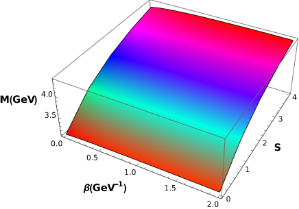
Figure 1: Mass of spectra for the charmonium for $\beta$ change with $S$ values

In Figure 1, we presented the mass change of charmonium for changing $\beta$ and $S$ values. It is seen that the increment in $S$ is more effective compared to the increment in $\beta$ in the sense of mass values.

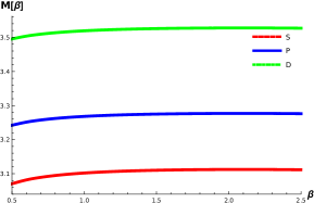
(a) $n=1$

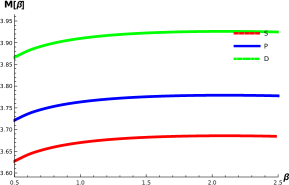
(b) $n=2$

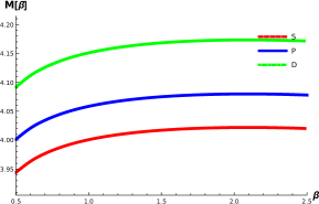
(c) $n=3$

Figure 2: Mass of spectra for the charmonium for different values of $L$

In Figure 2, we compared the mass values for different values of $n$ for $S,P$ and $D$. The value of mass is increasing with increasing $n$ and $L$ values. Also we conclude that the mass converges to its steady value with a sufficiently large $\beta$. Similar behaviors can be observed for the other thermodynamic quantities in Figure 3.

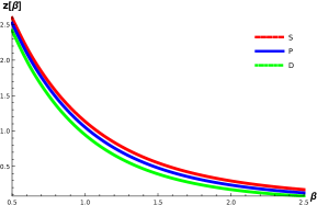
(a) Partial function

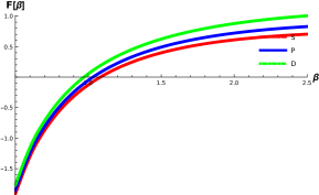
(b) Free Energy

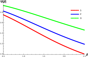
(c) Mean Energy

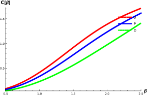
(d) Specific Heat

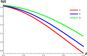
(e) Entropy

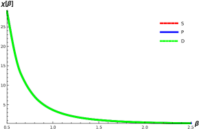
(f) Magnetic Susceptibility

Figure 3: Thermodynamic quantities for the charmonium for different values of $L$

Similar to charmonium, we calculated the mass values for different $L$ and $n$ for botomonium in Table 2. It is seen that the order of the mass values for charmonium and botomonium are almost equal to the order of the bare quark mass of $c$ quark ($m_{c}$) and the bare quark mass of $b$ quark ($m_{b}$) and agree with literature results. Due to the effect of the temperature dependent energy eigenvalue expansion formulations, small differences from the reference values are be observed. Also, as stated in [46] by Veliev et. al. the spectrum of bottomonium mass don’t change up to $T\simeq 100GeV$ but they start to diminish with increasing the temperature after this point in the framework of the QCD Sum rules.

Table 2: Numerical values mass of spectra for bottomonium (in $GeV$) for different values of $l$ and $n$ for $A=0.21\,GeV^{2}$, $B=1.560$, $C=2.15\times 10^{-3}GeV^{-1}$, $D=1.4\times 10^{-5}GeV^{3}$, $\delta=0.379\,GeV$, $m_{b}=4.823\,GeV$.

$\mathbf{n}$	$S$			$P$			$D$
	Present	Ref. [20]	Exp. [45]	Present	Ref. [20]	Exp. [45]	Present	Ref. [20]	Exp. [45]
1	$9.489$	$9.460$	$9.460$	$9.654$	$9.619$	$9.899$	$9.904$	$9.863$	$10.164$
2	$10.055$	$10.023$	$10.023$	$10.149$	$10.144$	$10.294$	$10.274$
3	$10.386$	$10.355$	$10.355$	$10.443$	$10.411$		$10.535$
4	$10.595$	$10.567$	$10.579$	$10.633$	$10.604$		$10.695$
5	$10.735$	$10.710$	$10.876$	$10.762$			$10.805$
6	$10.834$		$11.019$	$10.853$			$10.885$

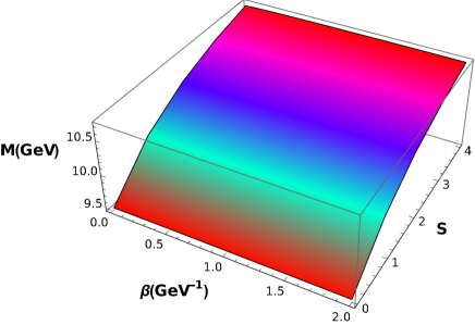
Figure 4: Mass of spectra for the bottomonium for $\beta$ change with $S$ values

In Figure 4, we displayed the mass change of bottomonium for changing $\beta$ and $S$ values. The similar behavior as in charmonium is also observed for the bottomonium.

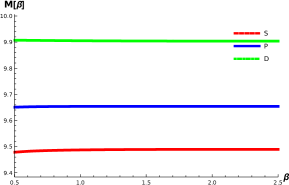
(a) $n=1$

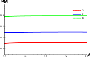
(b) $n=2$

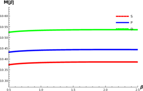
(c) $n=3$

Figure 5: Mass of spectra for the bottomonium for different values of $L$

As can be seen from Figure 5, similar to the charmonium, as the temperature ($T$) is getting smaller ($\beta$ increases) the mass values increase for all values of $n$ for the bottomonium but much higher values.

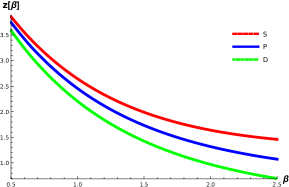
(a) Partial function

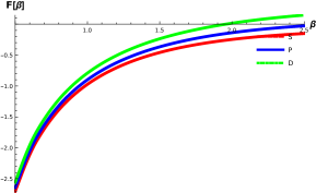
(b) Free Energy

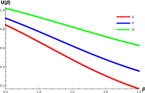
(c) Mean Energy

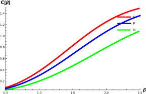
(d) Specific Heat

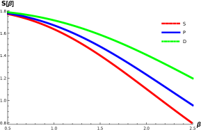
(e) Entropy

(f) Magnetic Susceptibility

Figure 6: Thermodynamic quantities for the bottomonium for different values of $L$

We displayed the change of the thermodynamic quantities with increasing values of the $\beta$ in Figure 6. Again it is seen that all of them are getting their steady values at a sufficiently large $\beta$ value and they also decrease except the free energy function and specific heat. For the high values of $\beta$, the entropy is getting very small [47]. There is a very little probability of transition to a higher energy level due to the occupation of the lowest level. Also with decreasing values of $\beta$, the entropy is very large. This behavior enforces the probability of the transition to go up. When all levels are occupied at small $\beta$ there is a little change in the entropy for small changes in $\beta$ and a lower heat capacity. Magnetic susceptibility efficiency drops off rapidly with $\beta$. As a result, for small $\beta$ values thermal effects are dominant and there is no response for the quantum phenomena in them.

Conclusion

In this article, the temperature dependent energy, mass and thermodynamic quantities (free energy $F(\beta)$, mean energy $U(\beta)$, specific heat $C(\beta)$, entropy $\mathcal{S}(\beta)$ and magnetic susceptibility $\chi(\beta)$ in terms of canonical partition function $Z(\beta)$) for quarkonia is calculated using the temperature dependent energy eigenvalue expansion. We calculated these quantities using the fixed values of bare quark masses and parameter sets and shown that these results agree with the literature. The effect of the temperature dependent energy eigenvalue expansion can be observed from the small differences in the numerical values compared to the experimental ones that use fixed temperature.The smallness of the difference means that it is worth introducing the temperature-dependence in the potential. Interesting results are obtained in the case of bottonium and charmonium in the sense of displaying the bound-state mass seems to be less sensitive to temperature changes. Also, the dependence of the thermodynamic quantities on $L$ is seen to be stronger on bottomonium than on charmonium. The results of the temperature dependent energy eigenvalue expansion can be improved by using similar parameter sets ($A,B,C,D$ and $\delta$) used for the experimental setup. Temperature has a positive effect on all of the thermal properties except the free energy. As a further study, it may be very interesting to extend this work to include spin-spin interactions, spin-orbital interaction or complex potential case. Also as another extension, one can consider the Shanon and Renyi entropies for quarkonia. These new results may be used in numerous practical purposes such as measuring the squeezing of quantum fluctuation and reconstruction of the charge and momentum, which are closely related to fundamental and experimentally measurable quantities.

Data Availability

No data were used to support this study.

Conflicts of Interest

The author declares no conflicts of interest.

Founding Statement

The author declare that this research did not receive any funding from any sources.

References

- [1] Domenech-Garret J L, and Sauchis-Lozano M A, 2008 Phys. Lett. B 669 52
- [2] Brambilla N, Eidelman S, Heltsley B, et al. 2011 Eur. Phys. J. C 71 1534
- [3] Kakade U and Patra B K, 2015 Phys. Rev. C 92 024901
- [4] Lakhina O and Swanson E S, 2006 Phys. Rev. D 37 014012
- [5] Cançelik Y and Gönül B, 2014 Mod. Phys. Lett. A 29 1450170
- [6] Mutuk H, 2018 Ad. in High Energy Phys. 5961031
- [7] Agotiya V K, Solonki S and Lal M, 2021 arXiv: 2105.12346(hep-ph)
- [8] De R, Dutt R and Sukhatme U, 1992 J. Phys. A: Math. Gen. 25 L843
- [9] Ixaru L G, Meyer H D and Berghe G V, 2000 Phys. Rev. E 61 3151
- [10] Sandin P, Ogren M and Gullikson M, 2016 Phys. Rev. E 93 033301
- [11] Okorie U S, Ikot A N and Edet C O, Rampho G J, Sever R and Akpan I O 2019 J. Phys. Commun. 3 095015
- [12] Edet C O, Okorie U S, Osobonye G, Ikot A N, Rampho G J and Sever R, 2000 J. Math. Chem. 58 989
- [13] Nikiforov A and Uvanov V B, 1988 Special Functions of Methematical Physics, (Birkhauser, Basel)
- [14] Alberico W M, Beraudo A, Pace A D and Molinari A, 2007 Phys. Rev. D 75 074009
- [15] Mocsy A and Petreczky P, 2007 Phys. Rev. Lett. 99, 211602
- [16] Abu-Shady M, Abdel-Karim T A and Ezz-Alarab Sh, 2019 J. of the Egyp. Math.Soc. 27 14
- [17] Ahmadov H I, Aydın C, Huseynova N Sh and Uzun O, 2013 Int. J. Mod. Phys. E 22 1350072
- [18] Ahmadov A I, Aydın C and Uzun O, 2014 Int. J. Mod. Phys. A 29 1450002
- [19] Ahmadov A I, Aydın C and Uzun O, 2019 J. of Phys.: Conf .Series 1194 012001
- [20] Ahmadov A I, Abasova K H and Orucova M Sh, 2021 Ad. High Energy Phys. 1861946
- [21] Klan G R, 2009 Eur. Phys. J. D 53 123
- [22] Pacheco M H, Landim R and Almeida C A S, 2003 Phys.Lett.A 311 93
- [23] Pacheco M H, Maluf RV, Almeida C A S and Landim R R, 2014 EPL 108 10005
- [24] Arda A, Tezcan C and Sever R, 2016 Eur.Phys.J.Plus 131 323
- [25] Arda A, 2017 Pramana-J.Phys. 88 39
- [26] Hassanabadi H and Hosseinpoura M, 2016 Eur. Phys. J. C 76 553
- [27] Matsui T and Satz H, 1986 Phys. Lett. B 178 416
- [28] Fingberg J, 1988 Phys. Lett. B 424 343
- [29] Karsch F, Mehr M T and Satz H, 1988 Z.Phys.C-Particles and Fields 37 617
- [30] Boliu Y B, 1996 Commun. Theor. Phys. 26 425
- [31] Brambilla N, Escobedo M A and Ghiglieri J, 2010 JHEP 1009 038
- [32] Asakawa M, Hatsuda T and Nakahara Y, 2003 Nucl. Phys. A 715 863
- [33] Döring M, Ejiri S, Kacmarek O, Karsch F and Laermann E, 2006 Eur. Phys. J. C 46 (179)
- [34] Abu-Shady M, Abdel-Karim T A and Klokha E M, 2018 Adv. High Energy Phys. 7356843
- [35] Boyd G, Engels J and Karsch F, 1996 Nucl.Phys.B 469 419
- [36] Brau F and Buesseret F, 2007 Physics Rev. C 76 05212
- [37] Pekeris C L, 1934 Phys.Rev. 45 98
- [38] Ferreira F L S and Prudente F V, 2013 Phys.Lett.A 377 3027
- [39] Kuchin S M and Maksimenko N V, 2013 Univ. Phys. Appl. 7 295
- [40] Kumar R, and Chamd F, 2013 Commun. Theor. Phys. 59 528
- [41] Benedetto J J and Zimmermann G and Fourier J, 1997 Anal.Appl. 3 505
- [42] Ikot A N, Lütfüoğlu B C, Nqwueke M I, Udoh M E, Zare S and Hasanabadi H 2016 Eur.Phys.J.Plus 131 419
- [43] Jia C S, Zhang L H and Wang C W, 2017 Chem.Phys.Lett. 667 211
- [44] Song X Q, Wang C W and Lia C S, 2017 Chem. Phys. Lett. 673 50
- [45] Zyla P A et al., 2020 Review of Particle Physics, to be published in Prog.Theor.Exp.Phys. 083C01
- [46] Veliev E V, Sundu H, Azizi K and Bayar M, 2010 Phys. Rev. D, 82 056012
- [47] Rastegar H R, Arda A and Sever R 2021 Optimal and Quantum Electronics, 53 3