Control of a qubit state by a soliton propagating through a Heisenberg spin chain

Abstract

We demonstrate that nonlinear magnetic solitary excitations – solitons – traveling through a Heisenberg spin chain may be used as a robust tool capable of coherent control of the qubit’s state. The physical problem is described by a Hamiltonian involving the interaction between the soliton and the qubit. We show that under certain conditions the generic Hamiltonian may be mapped on that of a qubit two-level system with matrix elements depending on the soliton parameters. We considered the action of a bright and a dark solitons depending on the driving nonlinear wave function. We considered a local interaction restricted the closest to the qubit spin in the chain. We computed the expressions of the physical quantities of interest for all cases and analyzed their behavior in some special limits.

I Introduction

The control of spin dynamics is a prerequisite for effective quantum computing and quantum information processing [1, 2, 3, 4, 5, 6]. The research in this field is focused on the physical implementation of the quantum computer, that relies on the realization of a two-level quantum system – the qubit. Over the last few decades, a number of two-level systems have enjoyed great interest as potential candidates for qubits. These include among other, the electrons confined in quantum dots due to their very long dephasing times and long phase coherence lengths [7], nanometer-scale magnetic particles or clusters with large total spin and high anisotropy [8], molecular magnets consisting of clusters with coupled transition metal ions [9] and a transmon-type superconducting qubit [10].

To manipulate the state of qubits, there are different approaches involving external stimuli, such as an electric field, a laser beam, a magnetic field or microwave pulses. The properties of systems composed of a qubit under the action of one of these stimuli have been the subject of extensive research (see Refs. [2, 10, 11, 6, 12, 13, 13, 14] and references therein). On the other hand, a scarcely explored path to alter the state of a qubit takes account of an effective well localized in space and time solitary wave propagating through a quantum spin chain – the soliton. Solitons are collective excitations that emerge in a variety of nonlinear systems spanning all branches of physics, such as optical fibers, cold atoms, fluids, magnets and so on. The study of nonlinear spin dynamics in magnetic materials related to different phenomena in condensed matter physics has been the subject of considerable interest for decades and a series of theoretical investigations [15, 16, 17, 18, 19, 20, 21, 22, 23, 24, 25, 26, 27, 28] has concentrated on unveiling the underlying mechanism of soliton formation in the framework of different magnetic models (for reviews the interested reader may consult Refs. [29, 30, 31, 32] and references therein). The ever growing interest in solitary spin waves that can travel under certain physical conditions with constant shape and velocity is also due to their applications in various technological fields, such as spintronics [33]. In this respect, there are only a few papers dealing with the control of the qubit by a soliton excitations propagating along a Heisenberg spin chain [34, 35, 36, 37, 38]. In this system, a solitary wave may be coherently generated by exciting the spin at one end of the chain via a time-dependent magnetic field. On the experimental side the potential coherent manipulation of a transmon–type superconducting qubit with the aid of a ferromagnetic single–magnon excitation in a millimeter-sized ferromagnetic sphere was considered in Ref. [10].

To explore the physics of a system consisting of an interacting soliton with a qubit, the traveling soliton is generated a distance apart from the qubit in order to reduce noise effects that might break quantum coherence. Moreover, the soliton parameters and the strength of the qubit-chain coupling may be tuned to control the qubit states. The qubit dynamics governed by a soliton propagating in a magnetic chain was numerically studied with the aid of the Bloch equations in Refs. [37, 38]. There, the chain was modeled by an anisotropic Heisenberg model with spin-spin interaction restricted either to nearest-neighbors or extended to include next to nearest-neighbors, assuming that the qubit does not affect the stability of the soliton, while the soliton may be used to control the behavior of the qubit. In the present paper, we tackle this problem in a more rigorous fashion and show that this assumption is indeed valid when the magnitude of the spin in the chain is sufficiently large. Hence, we demonstrate that in the large-spin limit the quantum problem reduces to the corresponding nonlinear Schrödinger equation for a two-level quantum system [3] for the qubit in the quasi-classical approximation, i.e. when the magnetic soliton stands for a large number of magnons [29]. We would like to anticipate that unlike familiar two-level quantum systems, the Hamiltonian derived here has a peculiar property that is all its matrix elements depend in a complex way on the soliton’s characteristics. On the other hand, the soliton is obtained as a solution of quasi-classical equations of motion for the spin chain described by the Heisenberg model with nearest-neighbor spin-spin interaction. Then, we proceed with the derivation of the approximated analytic solutions for the qubit, and find the probabilities for qubit switching. Our analysis of the physical problem shows that by a suitable choice of the parameters of the soliton it is possible to control the dynamics of the qubit.

This paper is organized as follows: The quantum model of interest is defined in Section II. In Section III, we demonstrate how the original problem reduces to the study of a quasi-classical two-level system. The effect of the quasi-classical solitons and possible ways to control the qubit state are analyzed in Section IV. To achieve our goal, we consider a local coupling of the qubit and its closest spin on the chain to study the effects of two types of solitons – bright and dark – on the behavior of the qubit. In the last Section V, we summarize our results.

II the Spin chain – Qubit system

The system of interest is composed of a qubit anisotropically interacting with an anisotropic Heisenberg spin chain. A general expression of the Hamiltonian reads

$$H= -J\sum_{n}\mathbf{S}_{n}\cdot\mathbf{S}_{n+1}-A\sum_{n}(S^{z}_{n})^{2}-\mu H_{0}\sum_{n}S^{z}_{n}$$

$$-d_{xy}\left[{S^{x}_{0}}{\sigma}^{x}+{S^{y}_{0}}{\sigma}^{y}\right]-d_{z}{S^{z}_{0}}{\sigma}^{z}-\nu H_{0}\sigma^{z}$$ (1)

with $\mathbf{S}_{n}\equiv(S_{n}^{x},S_{n}^{y},S_{n}^{z})$ – the spin operator located at the site $n$, $\boldsymbol{\sigma}\equiv\left(\sigma^{x},\sigma^{y},\sigma^{z}\right)$ is the half-spin operator associated to the qubit, to be dubbed hereafter “qubit” for short. The constants $J>0$ and $A>0$ stand for the spin coupling and the strength of the crystal field anisotropy, respectively. $H_{0}$ is an external magnetic field oriented along the $z$-direction. $\mu$ and $\nu$ are the magnetic moments per spin in the chain’s sites and the qubit, respectively. The interaction between the qubit and the spin chain is parametrized by the coupling’s components $d_{xy}$ within the $xy$ plane and $d_{z}$ along the $z-$axis. Here and below, we set $\hbar=1$, i.e. we work in units of $\hbar$ and assume that the qubit is coupled to the spin sitting at site $n=0$ of a long (quasi-infinite) spin chain with periodic boundary conditions, thus minimizing the effect of the boundaries on the properties of the chain.

It is convenient to express Hamiltonian (1) in terms of raising and lowering spin operators designated by “$+$” and “$-$”, respectively, i.e.

$$S_{n}^{\pm}=S^{x}_{n}\pm iS_{n}^{y}\quad\mathrm{and}\quad\sigma^{\pm}=\sigma^{x}\pm i\sigma^{y},$$

that obey the conventional spin commutation relations. Thus, it can be easily seen that the ensuing Hamiltonian possesses an invariant that is the $z$-projection of the total spin $\boldsymbol{\Sigma}=\mathbf{S}+\boldsymbol{\sigma}$ of the physical system – spin chain and qubit, i.e.

$$\Sigma^{z}=S^{z}+{\sigma}^{z}.$$

It is associated to the global $U(1)$ gauge symmetry $S^{\pm}_{n}\to S^{\pm}_{n}e^{\pm i\phi}$ and $\sigma^{\pm}\to\sigma^{\pm}e^{\pm i\phi}$, where $\phi$ is an arbitrary real constant. Thus, by adding and subtracting the term $\mu H_{0}\sigma^{z}$ to Hamiltonian (1), we end up with the invariant structure $-\mu H_{0}\Sigma^{z}$, which just shifts the energy scale, and after a subsequent phase transformation, it adds up to the phase of the state vector. Finally, the resulting Hamiltonian may be split into two components

$$H+\mu H_{0}\Sigma^{z}=H^{\text{c}}+H^{\text{q}},$$ (2a)

where

$$H^{\text{c}}=-J\sum_{n}\mathbf{S}_{n}\cdot\mathbf{S}_{n+1}-A\sum_{n}(S^{z}_{n})^{2}$$ (2b)

describes the magnetic properties of the Heisenberg spin chain in the absence of the external field, and

$$H^{\text{q}}=\left[(\mu-\nu)H_{0}-d_{z}{S^{z}_{0}}\right]\sigma^{z}-\frac{d_{xy}}{2}\left({S^{+}_{0}}{\sigma}^{-}+{S^{-}_{0}}{\sigma}^{+}\right)$$ (2c)

is associated to the qubit and its interactions with the external field $H_{0}$, as well as the chain.

Our main task here is to coherently modulate the qubit state through manipulation of the state of the spin chain. Thus, we find it more appropriate to work in the framework of the Heisenberg picture with respect to Hamiltonian (2b) using the transformation

$$|\psi(t)\rangle \to e^{iH^{\text{c}}t}|\psi(t)\rangle,$$ (3a)

$$H^{\mathrm{q}} \to e^{iH^{\text{c}}t}H^{\text{q}}\,e^{-iH^{\text{c}}t},$$ (3b)

where $|\psi(t)\rangle$ stands for the time dependent state vector. Then, the transformed Hamiltonian takes the expression (2c) by replacing the spin $\mathbf{S}_{0}$ with its time dependent counterpart.

III quasi-classical Approximation

The equations of motion of a spin sitting on the Heisenberg chain are given by

$$i\frac{\partial}{\partial t}\mathbf{S}_{n}=[\mathbf{S}_{n},H^{c}].$$ (4)

For the ladder operators, we have

$$\pm i\frac{\partial}{\partial t}S^{\pm}_{n}= -J\left[S^{z}_{n}\left(S^{\pm}_{n-1}+S^{\pm}_{n+1}\right)-S^{\pm}_{n}\left(S^{z}_{n-1}+S^{z}_{n+1}\right)\right]$$

$$+A\left(S^{z}_{n}S^{\pm}_{n}+S^{\pm}_{n}S^{z}_{n}\right).$$ (5)

For the purpose of this paper, we assume that the quantum number $S$ is large enough to consider the quasi–classical limit [39]. Therefore, we will work in the large-$S$ approximation where the physical properties of the spin chain obey the laws of classical mechanics. In this case the back-action of the qubit on the chain may be neglected. Such regime can always be achieved in the large-$S$ limit due to the fact that the spin–chain component $H^{c}$ scales as $S^{2}$ while the qubit component $H^{q}$ like $S$. Moreover, we assume that the deviation of the spin from its maximal projection, $S_{n}^{z}=S$, along the $z$-axis is small enough.

Within this quasi-classical approximation, the components of the spin operators transform into classical functions: $S_{n}^{+}=S\alpha_{n}$, $S_{n}^{-}=S\alpha_{n}^{*}$, $S_{n}^{z}=S\sqrt{1-|\alpha_{n}|^{2}}$. Substituting in (III), we get

$$i\frac{\partial\alpha_{n}}{\partial t}=\ 2AS\alpha_{n}\sqrt{1-|\alpha_{n}|^{2}}$$

$$-JS\left[(\alpha_{n+1}+\alpha_{n-1})\sqrt{1-|\alpha_{n}|^{2}}\right.$$

$$\ \left.\qquad-\alpha_{n}\left(\sqrt{1-|\alpha_{n+1}|^{2}}+\sqrt{1-|\alpha_{n-1}|^{2}}\right)\right].$$ (6)

A similar equation is obtained for the corresponding complex conjugate $\alpha^{*}$. To solve (III), we look for solutions in the form of amplitude–modulated waves, i.e.

$$\alpha_{n}(t)=\varphi_{n}(t)e^{\textstyle i(kn-\omega t)},$$ (7)

where $\varphi_{n}(t)$ denotes the envelope of $\alpha_{n}(t)$, $k$ – the wave number, $\omega$ – the angular frequency of the carrier wave. Notice that the phase of the functions $\alpha_{n}(t)$ is linear in both the position of the spin and time by virtue of the approximation of small spin deviations from their maximal projection along the $z$-axis.

For further analysis, we employ the semidiscrete approach [40, 41, 42, 43], i.e. we treat the phase factor exactly and use a continuum approximation for the envelope $\varphi_{n}(t)$. This removes the restriction for long carrier wavelengths and permits the study of envelope solitons with arbitrary wave numbers inside the Brillouin zone.

In the continuum limit, corresponding to a vanishing distance, say $\Delta x$, between nearest-neighbor spins on the chain with a large number of spins $N$, i.e. in the limit $\Delta x\to 0$ and $N\to\infty$, provided $N\Delta x$ remains finite, the discrete function $\varphi_{n}(t)$ may be approximated by the smoothly varying time dependent real function $\varphi(x,t)$ describing the deviation of the spin, located at a position $x$, with respect to the $z-$axis. Then, for wide excitations with width, $L\gg\Delta x$, and an envelope satisfying

$$[\varphi(x,t)]^{2}\ll 1,$$ (8)

Eq. (III) transforms into the nonlinear Schrödinger equation (NLSE)

$$i\left(\frac{\partial\varphi}{\partial t}+v_{g}\frac{\partial\varphi}{\partial x}\right)=(\omega_{0}-\omega)\varphi-b_{k}S\frac{\partial^{2}\varphi}{\partial x^{2}}+g_{k}S|\varphi|^{2}\varphi,$$ (9)

with $\omega_{0}=$ $-2g_{k}S$ – the characteristic frequency of the magnon, $v_{g}=2SJ\sin k$ – the group velocity of the carrier wave, $b_{k}=J\cos k$ – the dispersion coefficient, and $g_{k}=J(\cos k-1)-A$ – a nonlinear coefficient that incorporates the spin exchange and anisotropy interactions that are both nonlinear. It is worth mentioning that the sign of the quantity $b_{k}g_{k}$, that is a function of the anisotropy constant $A$ and the wave number $k$, determines the nature of the soliton solutions of NLSE (9). Thus, we have bright solitons for negative values ($b_{k}g_{k}<0)$, while for positive values ($b_{k}g_{k}>0$) dark solitons may be achieved. Bright and dark solitons, as exact solutions of the NLSE (9), have been studied intensively over the last few decades [44, 45, 46, 47]. Notice that, the ensuing soliton propagates, with a velocity $v_{g}$, over the distance $L$, during the period $T=\frac{L}{v_{g}}$. Below, we will investigate numerically the stability of the soliton structures, with the aid of the predictor-corrector algorithm. Moreover, the accuracy of the computations is controlled through the conservation of the envelope amplitude squared. More details on numerical techniques for the investigating the properties of bright and dark solitons can be found in Ref. [48].

Within our quasi-classical approach in the Heisenberg picture complemented with the phase transformation

$$e^{i(kx-\omega t)\,\sigma^{z}},$$ (10)

the time dependent Hamiltonian (2c) reduces to the effective two-state Hamiltonian, given by

$$H^{q}(t)=\frac{1}{2}\Omega(t)\left(\sigma^{-}+{\sigma}^{+}\right)+\Delta(t)\,\sigma^{z},$$ (11a)

where

$$\Omega(t)=-d_{xy}S\varphi(x,t)$$ (11b)

is the time-dependent coupling and

$$\Delta(t)=(\mu-\nu)H_{0}-d_{z}S\sqrt{1-\left[\varphi(x,t)\right]^{2}}+\omega,$$ (11c)

is the time-dependent detuning.

Within the above mentioned quasi-classical approach, the action of the soliton on the qubit is fully embodied in the parameters $\Omega(t)$ (11b) and $\Delta(t)$ (11c). From the physical point of view, Hamiltonian (11a) represents a two-level system perturbed under the action of the soliton. Here the coupling $\Omega(t)$ is related to the transition between both levels and the detuning $\Delta(t)$ stands for the difference in energy between these levels. It is worth noticing that the coupling $\Omega(t)$ is proportional to the in-plane anisotropic parameter $d_{xy}$ times the envelope $\varphi(x,t)$, while the detuning $\Delta(t)$ is a linear function of the anisotropic coupling $d_{z}$, the external magnetic field, as well as the frequency of the carrier wave.

To explore the dynamics of the effective Hamiltonian (11a), we work in the standard spin basis of the qubit, starting from the Schrödinger equation and after some lengthy but straightforward algebra, we end up with the Schrödinger equation for the probability amplitudes $C_{\pm}(s)$, associated to the states $\left|\pm\tfrac{1}{2}\right\rangle$, given by

$$i\frac{\text{d}}{\text{d}s}\begin{bmatrix}C_{-}(s)\\ C_{+}(s)\end{bmatrix}=\begin{bmatrix}-\Theta(s)&1\\ 1&\Theta(s)\end{bmatrix}\begin{bmatrix}C_{-}(s)\\ C_{+}(s)\end{bmatrix}.$$ (12)

Here, we follow a standard procedure commonly used in solving the dynamical problem of two-level systems [49, 50]. It consists of finding a solution of the time-dependent equations describing the evolution of the effective Hamiltonian (11a) with the aid of the reduced-time variable

$$s(t)=\frac{1}{2}\int_{0}^{t}\Omega(u)\,\text{d}u,$$ (13)

and the Stückelberg variable

$$\Theta(s)=\frac{\Delta[t(s)]}{\Omega[t(s)]}$$ (14)

with initial conditions

$$C_{-}[s(-t_{i})]=0,\quad C_{+}[s(-t_{i})]=1$$

i.e. at $t=-t_{i}$, the qubit points in the $z$-direction.

We find this description of the considered two-level system problem more convenient, since a single $s$-dependent quantity in the Hamiltonian matrix $H(s)$ will make the subsequent analysis more transparent, although it does not fully decouple the Schrödinger equation (12).

IV Soliton-Driven Qubit Dynamics

We examine the effect of the two different sorts of solitons – bright and dark – propagating through an anisotropic Heisenberg spin chain on the qubit a distance apart from the spins. So far, we established that the corresponding general problem reduces to the two-level system problem for the qubit (12), where the soliton state characteristics are encoded in the variables (13) and (14) through the coupling (11b) and the detuning (11c).

IV.1 Bright–soliton drive

When $b_{k}g_{k}<0$, for an infinite chain subjected to the boundary conditions $|\varphi_{b}(x,t)|^{2}\rightarrow 0$ as $x\rightarrow\pm\infty$, the solution of NLSE (9) is a bright soliton given by

$$\varphi_{b}(x,t)=\varphi_{b0}\,{\rm sech}\,\frac{x-vt}{L}$$ (15a)

with amplitude

$$\varphi_{b0}=\frac{1}{L}\sqrt{\frac{2J\cos k}{J(1-\cos k)+A}},$$ (15b)

and frequency

$$\omega_{b}=\omega_{0}-2SJ\frac{\cos k}{L^{2}}.$$ (15c)

That is, the soliton frequency is shifted relative to the linear spin wave frequency $\omega_{0}$. Further, we may choose the wave number $k$ and soliton width $L$ ($L\gg\Delta x$) as running soliton parameters of both bright and dark solitons. The domain of existence of the bright soliton solution (15a) in the case of an easy axis anisotropy ($A>0$), is $0\leq k<\tfrac{\pi}{2}$. Notice that the soliton is at rest when $k=v=0$. Bright soliton solutions expressed by (15a) for a one-dimensional system of classical spins with nearest neighbour Heisenberg interaction were obtained and analyzed in details in Refs. [51, 52].

The propagation of a bright soliton generated at initial time $t=0$ away from the qubit position has been investigated via numerically solving the system of discrete equations of motion (III). We used a chain composed of 1000 spin sites, $J=S=1$, $A=3$ and periodic boundary conditions (see Fig. 1). It is easily seen that the bright solitary wave remains stable during its evolution in time throughout the spin chain.

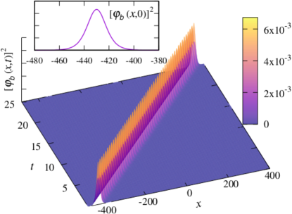
Figure 1: Time evolution of the square of the bright soliton solution, $[\varphi_{b}(x,t)]^{2}$, given by (15a) using the parameters $k=0.015708$ and $L=10$ for $S=J=1$ and $A=3$. The numerical analysis demonstrates that the soliton solution remains stable over time while propagating throughout the ferromagnetic Heisenberg spin chain. In the inset, we show the shape of the solitary wave as a function of the position on the spin chain at the initial time $t=0$.

For a bright soliton propagating in the chain and a qubit coupled to a single chain spin, the variables (13) and (14) are explicitly given by

$$s_{b}(t)=\Omega_{b0}T\left(\arctan e^{\frac{t}{T}}-\frac{\pi}{4}\right),$$ (16a)

and

$$\Theta_{b}(s)=-\frac{\Delta_{b0}}{d_{xy}S}\,\,\tilde{\varphi}_{b}(s)^{-1}-\frac{d_{z}}{2d_{xy}}\,\,\tilde{\varphi}_{b}(s),$$ (16b)

where the amplitude of the coupling (11b) is now expressed by

$$\Omega_{b0}=-d_{xy}S\varphi_{b0},$$ (16c)

the time-independent term of the detuning (11c) reads

$$\Delta_{b0}=(\mu-\nu)H_{0}-d_{z}S+\omega_{b}$$ (16d)

and

$$\tilde{\varphi}_{b}(s)=\varphi_{b}[t(s)]=\varphi_{b0}\cos\left(\frac{\pi}{2}\frac{s}{s_{\infty}}\right).$$ (16e)

In this case, we placed the qubit at $x=0$, and expanded the square root in the detuning (11c) in Taylor series up to the first order with respect to the function $\tilde{\varphi}_{b}(s)^{2}\propto\varphi_{b0}^{2}\ll 1$. This implies that when

$$|\Delta_{b0}|\gg\frac{1}{2}\,|d_{z}|S\varphi_{b0}^{2},$$ (17)

we can safely neglect the second term in (16b) to end up with

$$\Theta_{b}(s)=\frac{\Delta_{b0}}{\Omega_{b0}}\,{\rm sec}\left(\frac{\pi}{2}\frac{s}{s_{\infty}}\right),$$ (18)

that is identical to the Stückelberg variable of the Rosen-Zener model [53] with coupling $\Omega_{b0}\mathrm{sech}\left(\tfrac{vt}{L}\right)$ and time-independent detuning (16d). Thus, within this approximation there is a direct mapping of our model onto Rosen–Zener’s one. Then, the solution for the final time spin-flip probability is given by

$$P_{-}=P_{-}(+\infty)\approx\frac{\sin^{2}\left(\frac{\pi}{2}\Omega_{b0}T\right)}{\cosh^{2}\left(\frac{\pi}{2}\Delta_{b0}T\right)}.$$ (19)

Whence the transition probability exhibits oscillations with amplitude $\cosh^{-2}\left(\frac{1}{2}\pi\Delta_{b0}T\right)$ as a function of the zero–mode interaction $\int_{-\infty}^{\infty}\Omega_{b}(t)e^{-i0t}dt=\pi\Omega_{b0}T.$ With the proper choice of control parameters, one may create superposition states satisfying the inequality

$$|C_{-}(+\infty)|\cosh\left(\frac{1}{2}\pi\Delta_{b0}T\right)\leq 1,$$

given that condition (17) is fulfilled. However, a qubit-flip for $\Delta_{b0}\neq 0$ is not possible since the amplitude $C_{-}(+\infty)$ decays exponentially as a function of $\Delta_{b0}T$.

Remark that a control over the magnitude of the transition probability can be achieved on-resonance, i.e. when

$$\Delta_{b}(t)=0,$$ (20)

then, we have

$$P_{-}=\sin^{2}\left(\frac{\pi}{2}\,\Omega_{b0}T\right).$$ (21)

Since the detuning is a time-dependent quantity, while we assume that the tuning parameters are time-independent, the resonance condition (20) cannot be satisfied. Therefore, we shall rather seek to achieve an effective on-resonance regime. This requires to take into account the fact that the term $\tilde{\varphi}_{b}(s)^{2}$ cannot be neglected and (17) does not need to be fulfilled. To proceed further, we choose the coupling $d_{z}$ to be a tunable parameter and split it into two components

$$d_{z}=d_{z0}+d_{z1},$$ (22a)

with the time-independent quantity

$$d_{z0}=\frac{1}{S}\left[\omega_{b}+(\mu-\nu)H_{0}\right],$$ (22b)

obtained by setting $$\Delta_{b0}\equiv\lim_{t\to-\infty}\Delta_{b}(t)=0$$. The detuning time dependence, on the other hand, is effectively taken care of via the expression

$$d_{z1}=\frac{d_{z0}}{2}\,\left(\frac{\varphi_{b0}}{\eta}\right)^{2},$$ (22c)

where $\eta$ is a suitably chosen dimesionless running parameter of the order of unity. Expression (22c) approximately fulfils (20), which holds only during the time period (of the order of $T$) when the soliton interacts with the qubit, i.e. when a transition takes place. At early and late times, in the absence of interaction, the system is slightly detuned, altering nothing but the phases of the amplitudes. The “relaxed” requirement (22) provides a more accurate approximation to the on-resonance regime (20) than the strict setting $\Delta_{b}=0$, moreover it allows the use of the transition probability formula (21).

In general, the effective resonant coherent control can be accomplished by demanding that

$$P_{-}=\xi,\quad 0\leq\xi\leq 1,$$ (23a)

yielding

$$\pi\Omega_{b0}T=\pm\,2\arcsin\sqrt{\xi}-2p\pi,\quad p\in\mathbb{Z},$$ (23b)

for the zero-mode interaction. In particular, in order to achieve properties, such as complete population transfer (qubit switching) $P_{-}=1$, complete population return (qubit switching with consecutive qubit return) $P_{-}=0$, and equal superposition $P_{-}=\frac{1}{2}$, we require that the zero-mode interaction fulfills $\pi\Omega_{b0}T=(2p+1)\pi,\,2p\pi$ $(p\neq 0)$, and $\left(p+\frac{1}{2}\right)\pi$, where $p\in\mathbb{Z}$, respectively.

To ensure the fulfillment of (23) we can choose the coupling $d_{xy}$ to be a tunable parameter, that satisfies (16c) with $\Omega_{b0}$ from (23b). To summarize, the manipulation of the values of the spin chain – qubit coupling components $d_{z}$ (22) and $d_{xy}$ (16c) at given soliton parameters allows to establish an effective on-resonance coherent control over the state of the qubit.

The dynamics of the probabilities $P_{\pm}(t)=|C_{\pm}[s(t)]|^{2}$ for the case of qubit switching at some specific values of the soliton parameters is shown in Fig. 2. The necessity of the correction parameter $d_{z1}$ expressed in (22c) is evident from the comparison of the probabilities for the effective on-resonance model with $d_{z1}\neq 0$ and without correction ($d_{z1}=0$), and the exact probabilities numerically obtained from (12). It is clearly seen that the correction term successfully cures the deficiency introduced by solely using the static term $d_{z0}$ in Eq. (22b).

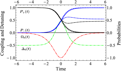
Figure 2: Effective resonant qubit switching dynamics. Upper panel: Probabilities for the qubit states, numerically obtained by solving (12), are plotted – $P_{+}(t)$ in black and $P_{-}(t)$ in blue. The solid and dashed curves depict the exact and approximated via $\left[\sqrt{1-\varphi(t)^{2}}\approx 1-\frac{1}{2}\varphi(t)^{2}\right]$ probabilities, with correction determined by $d_{z1}$ (22c). The dash-dotted curves correspond to the noncorrected probabilities at $d_{z1}\equiv 0$. Lower panel: The coupling $\Omega_{b}(t)$, $(\Omega_{b0}T=-1)$, and the corrected detuning $\Delta_{b}(t)$ are shown with dash-dotted red and dash-dotted green, respectively. The parameters used for computations are $S=10$, $L=10\Delta x$, $k=\frac{\pi}{30}$, $\mu=\nu$, $JT=4.783$, $AT=47.834$, $d_{xy}T=2.243$, $d_{z1}T=0.051$ with $\eta=1.372$. The dimensionless time $t/T$ is plotted on the abscissa.

It is worth noting that the relative phase between the amplitudes $C_{\pm}(+\infty)$ in the effective resonance regime is altered and oscillates with time due to the correction term. In the non-corrected probabilities the phase of the solution is time-independent. The relative phase in the superpositions of qubit states contains an additional phase of $2\omega_{b}t$ as a consequence of the phase transformation (10).

IV.2 Dark–soliton drive

The dark soliton solution of NLSE (9) that exists for $b_{k}g_{k}>0$ ($A>0$ and $\frac{\pi}{2}<k\leq\pi$) with the amplitude taking the same value at both ends of the chain, i.e. $x\rightarrow\pm\infty$ reads

$$\varphi_{d}(x,t)=\varphi_{d0}\,{\rm tanh}\left(\frac{x-vt}{L}\right)$$ (24a)

with amplitude

$$\varphi_{d0}=\frac{1}{L}\sqrt{-\frac{2J\cos k}{J(1-\cos k)+A}}\,$$ (24b)

and frequency

$$\omega_{d}=\omega_{0}+2SJ\frac{\cos k}{L^{2}},$$ (24c)

where the second term describes the correction to the frequency of the linear spin wave. Notice that at $k=\pi$, thus $v=0$, we have a static dark soliton. It is worth mentioning that spin-wave dark solitons have been theoretically predicted and experimentally realized [54, 55, 56].

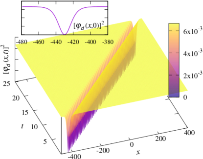
Figure 3: Time evolution of the square of the dark soliton solution $[\varphi_{d}({x,t})]^{2}$ in (24a) computed with the set of parameters $k=\pi-0.015708$ and $L=10$ for $S=J=A=1$. It is clearly seen that the soliton preserves its shape while propagating along the ferromagnetic Heisenberg chain. The inset shows the profile of the solitary wave as a function of the position on the spin chain at the initial time $t=0$.

We have investigated the evolution of a propagating dark soliton numerically based on the discrete equations of motion (III), and as in the case of bright soliton, it is generated at time $t=0$ away from the qubit position. Our numerical simulation have been performed on a chain with 1000 spin sites with $J=S=A=1$ under periodic boundary conditions. Remark that the dark solitary wave does not alter during the propagation along the chain (see Fig. 3).

When a dark soliton propagates in the chain and the qubit is coupled locally to a spin on the Heisenberg chain, the variables (13) and (14), respectively, read

$$s_{d}(t)={\rm sgn}(t)\,\frac{\Omega_{d0}T}{2}\,\ln\cosh\left(\frac{t}{T}\right),$$ (25a)

and

$$\Theta_{d}(s)=-\frac{\Delta_{d0}}{d_{xy}S}\,\,\tilde{\varphi}_{d}(s)^{-1}-\frac{d_{z}}{2d_{xy}}\,\,\tilde{\varphi}_{d}(s),$$ (25b)

where the amplitude of the coupling (11b) now reads

$$\Omega_{d0}=d_{xy}S\varphi_{d0},$$

while the time-independent term of the detuning (11c) is given by

$$\Delta_{d0}=(\mu-\nu)H_{0}-d_{z}S+\omega_{d}$$

and

$$\tilde{\varphi}_{d}(s)=-\varphi_{d0}\left[1-\frac{e^{-2f(s)}}{1+{\rm sgn}(s)\sqrt{2e^{-f(s)}\sinh{f(s)}}}\right],$$

with

$$f(s)=\frac{2}{\Omega_{d0}T}\ {\rm sgn}(s)\ s.$$

In order to obtain an invertible transformation between time $t$ and the variable $s$ (13) on the entire real axis, we used the sign function in (25a). Moreover, it can be easily seen that this transformation remains smooth.

Similar to the case of bright soliton, the qubit is set at the position $x=0$, and the square root in the detuning (11c) is expanded in Taylor series with respect to $\tilde{\varphi}_{d}(s)^{2}$. The second term in (25b) is of order $O(\varphi^{2}_{d0})$ compared to the first one, and can be neglected given that the counterpart of (17) for the dark soliton is fulfilled. Then, the problem reduces to the study of a model with hyperbolic tangent coupling

$$\Omega_{d}(t)=\Omega_{d0}\tanh\frac{t}{T},$$ (26a)

and constant detuning

$$\Delta_{d}(t)=\mathrm{const.}$$ (26b)

This is the so called “$\tanh$” model, that is exactly solvable and its physical properties are well known [57]. In the following, we will take advantage of the analysis of Ref. [57] to gain insights into the effect of the dark soliton on the behavior of the qubit. Let us point out that the model considered in Ref. [57] is restricted to positive times, while here we extend the study over the whole real time axis.

The probability $P_{-}(t)$ of the qubit flip may take any value in the interval $[0,1]$ for suitably chosen control parameters. For instance, it is possible to achieve a return of the qubit to its initial state. Furthermore at effective resonance, $\Delta_{d}=0$, both a return to the initial state and a qubit switch are possible. We will focus on the limiting cases of fast $\left(\frac{t}{T}\gg 1\right)$ and slow $\left(\frac{t}{T}\ll 1\right)$ solitons reflected by the behavior of the coupling’s tanh function and resonance. These are of particular interest since they provide analytical closed-form solutions in terms of some elementary mathematical functions. For further consideration, we assume that the interaction time of the soliton with the qubit is symmetric with respect to the reference time $t=0$, except for the resonance case.

The fast soliton is characterized by a ${\rm sgn}(t)$-dependent constant coupling

$$\Omega_{d}(t)\sim\tanh\left(\frac{t}{T}\right)\approx{\rm sgn}(t),\quad t\gg T.$$ (27)

The large–$S$ assumption ensures the fulfillment of the above condition that holds for a large set of combinations of the soliton’s parameters. After some lengthy, but straightforward computations, under the assumptions $|\Delta_{b}T|\ll 1$, $|\Omega_{b0}T|\ll 1$, $\Omega_{d0}\sim\Delta_{d}$ and for some specific values of $t$, the leading behavior of the transition probability takes the form

$$P_{-}(t)\sim P^{0}_{-}\left[\sin^{2}\,\frac{\chi(t)}{2}+\frac{1}{4}\sin^{2}\chi(t)\right],$$ (28)

where the amplitude and the phase read

$$P^{0}_{-}=\left(2\frac{\Omega_{d0}\Delta_{d}}{\Omega_{d0}^{2}+\Delta_{d}^{2}}\right)^{2}\sim 1,$$

and

$$\chi(t)=-\Omega_{d0}t,$$

respectively.

A peculiar feature of the transition probability $P_{-}(t)$ is that it consists of the superposition of two oscillating time-dependent components possessing different frequencies and amplitudes $\chi(t)$ and $\frac{1}{2}\chi(t)$. Eq. (28) implies that this behavior provides the opportunity to tune $P_{-}(t)$ to a specific preselected value, even close to unity. In this approximation, the transition probability $P_{-}(t)$ tends to the Rabi model probability with a jump through change of the sign of the coupling.

In the regime where $|\Delta_{d}T|$ is finite and $|\Omega_{d0}T|\ll 1$, we have $P_{-}(t)\propto\left(\frac{1}{2}\Omega_{d0}T\right)^{2}$, and hence such regime is not of interest, when one needs to achieve an appreciable qubit flip probability.

Let’s point out, that the case $|\Delta_{d}T|\ll 1$ and finite $|\Omega_{d0}T|$ related to the zeroth order approximation of $P_{-}(t)$ is contained in the general resonance solution (31), which vanishes in a symmetric time interval.

The limiting case $T\gg t$ is typical for a slow soliton, and hence, by a linear time-dependent coupling:

$$\Omega_{d}\sim\tanh\left(\frac{t}{T}\right)\approx\frac{t}{T},\quad t\ll T.$$ (29)

This behavior shows up as $k\rightarrow\pi$. Then, the tanh model may be mapped onto the Landau-Zener model rotated by $\frac{\pi}{4}$ that has been investigated in details in Ref. [58].

We consider the regime of sufficiently large coupling amplitude, i.e. $\Omega_{d0}\ t^{2}\gg T$ and the two limiting cases: $|\Delta_{d}T|\ll 2\Omega_{d0}t$ corresponding to a small detuning regime and $|\Delta_{d}T|\gg 2\sqrt{\Omega_{d0}T}$ associted to the large detuning regime. Here, the transition probabilities $P_{-}(t)$ are oscillatory and can be controlled to some extent by the soliton’s tunable parameters. Let’s point out that the case of large detuning case corresponds to the adiabatic solution. On the other hand, the case of weak coupling regime $\Omega_{d0}\ t^{2}\ll T$ is not of interest, due to the negligibly small qubit flip probability.

Finally we will turn our attention to the on–resonance ($\Delta_{d}=0$) regime, when the variable (25b) reduces to the second term only. Then, the detuning, $\Delta_{d}(t)\propto|\varphi_{d}(t)|^{2}\ll 1$, may be neglected, since it is almost zero in the region where the tanh-shaped coupling changes its sign, and it is vanishingly small elsewhere. In this effective on-resonance regime the transition probability reads

$$P_{-}(t)\approx\sin^{2}\left[\frac{1}{2}\Omega_{d0}T\,\ln\,\frac{\cosh\left(t/T\right)}{\cosh\left(t_{\rm i}/T\right)}\right].$$ (30)

It can be well approximated by the resonance Rabi model solution

$$P_{-}(t)\approx\sin^{2}\left(\frac{\Omega_{d0}\tau}{2}\right),\,\,t,t_{i}\gtrsim T,\,\,\tau=t-t_{\rm i}.$$ (31)

Indicating that, the evolution of the qubit undergoes slightly chirped oscillations with almost unit amplitude. Therefore, a qubit switch ($\Omega_{d0}\tau=(2p+1)\pi,\,p\in\mathbb{Z}$) and a return ($\Omega_{d0}\tau=2p\pi,\,p\in\mathbb{Z}$) of the qubit to its initial state, and superpositions of qubit states are possible to achieve for some specifically chosen controlable parameters. In particular, the choice of a symmetric time interval $t_{i}=t$ would always lead to a return of the qubit, because in resonance an anti-symmetric coupling function in symmetric interval produces $\Omega_{d0}\tau=0$.

V Conclusions

Manipulating the state of a qubit is crucial to quantum computing and quantum information processing. This may be achieved with the aid of an external stimulus. Here we consider the action of an anisotropic Heisenberg spin chain on a qubit placed a distance apart to get rid of the effect of decoherence (information loss) due to the backward effect of the qubit on the spin chain. To achieve our goal, we work in the large-spin approximation that allows us to map the original chain – qubit Hamiltonian onto a two–level problem of a qubit under the action of a propagating through the chain magnetic solitary wave. Thus, we may take control over the qubit state by tuning the soliton parameters. Here, we demonstrate the possibility to control the qubit state through a bright soliton or its dark counterpart. It is shown, among other, that the qubit can be flipped and/or returned in its initial state, and an equal superposition of qubit ‘up’ and ‘down’ states can be generated.

In the case of a local interaction of the qubit with its closest spin on the chain, the off-resonance and effective resonance regimes are studied. In all cases the considered problem is mapped onto some exactly solvable models. To achieve an effective resonance regime for a bright soliton a fine tuning of the $z$-component of the qubit coupling is required, while in the case of dark soliton this is not needed due to the smallness of the coupling around the time origin.

Finally, we believe that such a scheme for control of qubit by solitons may find application in systems, such as magnetic chains coupled to an artificially designed effective half-spin or a coherent atomic spin chain coupled to an artificially designed effective qubit.