Formal Privacy for Partially Private Data

Abstract

Differential privacy (DP) quantifies privacy loss by analyzing noise injected into output statistics. For non-trivial statistics, this noise is necessary to ensure finite privacy loss. However, data curators frequently release collections of statistics where some use DP mechanisms and others are released as-is, i.e., without additional randomized noise. Consequently, DP alone cannot characterize the privacy loss attributable to the entire collection of releases. In this paper, we present a privacy formalism, $(\epsilon,\{\Theta_{z}\}_{z\in\mathcal{Z}})$-Pufferfish ($\epsilon$-TP for short when $\{\Theta_{z}\}_{z\in\mathcal{Z}}$ is implied), a collection of Pufferfish mechanisms indexed by realizations of a random variable $Z$ representing public information not protected with DP noise. First, we prove that this definition has similar properties to DP. Next, we introduce mechanisms for releasing partially private data (PPD) satisfying $\epsilon$-TP and prove their desirable properties. We provide algorithms for sampling from the posterior of a parameter given PPD. We then compare this inference approach to the alternative where noisy statistics are deterministically combined with Z. We derive mild conditions under which using our algorithms offers both theoretical and computational improvements over this more common approach. Finally, we demonstrate all the effects above on a case study on COVID-19 data.

Keywords: data privacy, optimal transport, approximate Bayesian computation

1 Introduction

Differential privacy (DP) (Dwork et al., 2006b, 2014), a framework for releasing statistical outputs with provable privacy guarantees, has earned its popularity through its desirable properties such as robustness to post-processing and methodological transparency. DP offers semantic interpretations about what adversaries can learn in excess of their prior information, via Pufferfish (Kifer and Machanavajjhala, 2014), or by comparing information gains counterfactually based on whether an individual’s data was used via coupled worlds Bassily et al. (2013) or posterior-to-posterior semantics (Kasiviswanathan and Smith, 2008). These semantics describe privacy loss attributable to the DP mechanism, regardless of other arbitrary prior information. In recent years, there has been a massive proliferation of DP methods, with notable developments in private selection problems (McSherry and Talwar, 2007; Reimherr and Awan, 2019; Asi and Duchi, 2020), statistical inference tasks (Awan and Slavković, 2018; Canonne et al., 2019; Biswas et al., 2020), and synthetic data generation (Snoke and Slavković, 2018; Torkzadehmahani et al., 2019; McKenna et al., 2018).

In the central trust model, a centralized data curator processes all statistics published using data from a single confidential database. DP can only guarantee finite total privacy losses for a collection of outputs in the setting where each non-trivial output is released via a DP mechanism. However, data curators often release a collection of statistics where some are published with DP mechanisms and others are not. In these settings, DP can describe the privacy loss attributable to the outputs released with DP mechanisms, but this fails to non-trivially describe the privacy guarantees of everything the data curator actually released. Our central goal in this paper is to recover some formal privacy guarantees when DP does not meaningfully describe the entirety of the data curator’s actions due to the presence of what we call “public information,” i.e., statistics derived from the confidential database available without privacy-preserving randomized noise needed to satisfy DP. We investigate the unique problems associated with partially private data (PPD), data releases which contain both public information and query responses sanitized for formal privacy preservation.

There are many different circumstances in which PPD can arise; we briefly list some important cases. First, data curators may be legally or contractually bound to release public information along with their private releases. For tabular count data, public summary statistics may be released as-is, such as mariginal summaries (Slavković and Lee, 2010; Abowd et al., 2019b) or survey methodology descriptions in data sharing agreements (Seeman and Brummet, 2021). Similarly, data curators may make database schema and modeling decisions non-privately, such as choosing tuning parameters or setting privacy budgets based on particular utility goals (Xiao et al., 2021). Second, information about the database sample may be public prior to implementing formally private methodology. Most data curators do not currently use DP methods, posing unresolved challenges in reconciling future releases with past ones when results are temporally autocorrelated (Quick, 2021). These problems affect countless data curators, and it poses a significant barrier to wider adoption of privacy-preserving methodology when DP fails to describe what data curators are actually releasing in practice.

1.1 Contributions

In this paper, we present a privacy formalism, $(\epsilon,\{\Theta_{z}\}_{z\in\mathcal{Z}})$-Pufferfish ($\epsilon$-TP for short when $\{\Theta_{z}\}_{z\in\mathcal{Z}}$ is implied), which is a collection of Pufferfish (Kifer and Machanavajjhala, 2014) mechanisms indexed by realizations of a random variable $Z$. This variable represents public information about the confidential data not protected with DP noise. Recall that Pufferfish considers comparisons not of adjacent databases (as in DP), but conditional distributions given information about the confidential database; our framework considers these same distributions, but additionally conditioned on the realization of public information $Z=z$ that we happen to observe.

Our contributions are as follows. 1) We prove that $\epsilon$-TP maintains similar properties and semantic interpretations as DP (Lemmas 4 through 7). 2) We propose two release mechanisms for PPD, the Wasserstein Exponential mechanism (Theorem 9 generalizing (McSherry and Talwar, 2007)) and Wasserstein $K$-norm gradient mechanisms (Theorem 10 generalizing (Reimherr and Awan, 2019)), and prove their useful properties. 3) we provide algorithms for sampling from the posterior of a parameter given PPD, based on rejection and importance sampling (Algorithms 1 and 2, respectively). 4) We then compare this inference approach to the common alternative where noisy statistics are deterministicly combined with public information. We then derive conditions where our mechanisms require adding asymptotically less noise (Corollary 13) and offer stochastic improvements in inferential quality (Theorem 15). 5) Finally, we demonstrate all the effects above on a case study on COVID-19 data (Section 4).

Broader Impacts: Organizations hoping to share formally private results are frequently required to release results in a non-DP manner about the same database, even if the exact correspondence is not deterministic (for example, statistics based on a random sample from the database). We argue that this case warrants special attention because unlike the examples given in Dwork et al. (2017), which correctly states that population-level inferences about individuals cannot be quantified as privacy violations, here the data curator is directly in charge of multiple releases from the same database, only some of which may satisfy DP. This is a problem for which DP alone offers no substantive solutions other than to narrow the scope of which privacy losses are quantified. In this paper, we argue against this approach, as it fails to hold data curators accountable for additional privacy risks emanating from non-DP releases. We may hope that in the future, organizations are better equipped to implement DP as intended. Until such a time when organizations’ data processing requirements can accommodate DP, our work provides a solution to a real and present formal privacy problem.

1.2 Related literature

Research in DP, synonymous with (Dwork et al., 2006b), has spurned hundreds of similar definitions (Desfontaines and Pejó, 2019). Some of those (e.g., Pufferfish privacy (Kifer and Machanavajjhala, 2014), Blowfish privacy (He et al., 2014), coupled worlds privacy (Bassily et al., 2013), and dependent differential privacy (Liu et al., 2016)) can be extended to accommodate certain kinds of public information. We also note that extensions of Pufferfish have been used to address other conceptual issues with DP, such as accounting for non-individual database attribute disclosure risks (Zhang et al., 2020).

Our framework differs in a few key ways. First, these previous frameworks offer guarantees that do not change contextually based on the realized value of the public information. This is why we cannot naively apply Pufferfish to our problem, because the space of candidate conditional distributions for our database changes based on the realized value of $Z$; we need not consider a “worst-case” public information realization among all possible values of $Z$ when the realization is known publicly. Second, by treating public information as a random variable, we consider the effects of probabilistic public information by smoothly interpolating between the best case scenario (in which $X$ and $Z$ are entirely independent) and the worst case scenario (in which $X$ and $Z$ are perfectly correlated).

Existing works on formal privacy in the presence of public information typically focus on congeniality, or agreement between results derived from private and public information (Barak et al., 2007; Hay et al., 2010; Ding et al., 2011; Abowd et al., 2019a). Attempts to reinterpret these guarantees with semantic similarity to DP have been studied in (Ashmead et al., 2019; Gong and Meng, 2020). Our work does not require congeniality, but we prove that our proposed mechanisms can satisfy it. Recent work has also considered mechanism design in the presence of additional public information (Bassily et al., 2020) and provides helpful theoretical bounds, but it requires that the private and public samples are independently and identically distributed (iid). We relax the iid assumption, since our interest is in changes to mechanism design and valid statistical inference explicitly due to dependencies between private and public information.

2 Privacy guarantees of joint private and public releases

We provide all complete proofs in Appendix A. Throughout this paper, we consider a parameter of interest $\theta\in\Theta$, confidential database $X\in\mathcal{X}^{n}$, public information $Z\in\mathcal{Z}$, and sanitized private release $Y\in\mathcal{Y}$. In some cases, we consider $Y^{*}=h(Y,Z)$, where $Y^{*}$ post-processes both $Y$ and $Z$ according to the arbitrary function $h$. This is the approach taken by the Geometric mechanism (Ghosh et al., 2012), the Top-Down algorithm (Abowd et al., 2019b), and private hypothesis testing (Canonne et al., 2019), among many other methods.

2.1 Motivation: $\epsilon$-DP semantics with public information

In this section, we motivate why we want to characterize the privacy loss attributable to both $Y$ and $Z$ simultaneously. We first review $\epsilon$-DP in its original formulation. Note that in this Subsection 2.1, for notational ease, we temporarily assume that the distributions in question admit mass functions.

Definition 1 ($\epsilon$-DP (Dwork et al., 2006b, a))

Let $x\in\mathcal{X}^{n}$ and let $x^{\prime}\in\mathcal{X}^{n}$ be any database created by modifying one entry in $x$. A randomized algorithm $\{M(x):x\in\mathcal{X}^{n}\}$, i.e., a collection of probability distributions over $\mathcal{Y}$ indexed by elements of $\mathcal{X}^{n}$, satisfies $\epsilon$-DP iff for all such $x,x^{\prime}$ and $y\in\mathcal{Y}$.

$$\operatorname{\mathbb{P}}(M(x)=y)\leq\operatorname{\mathbb{P}}(M(x^{\prime})=y)e^{\epsilon}.$$ (1)

As presented in Equation 1, DP is a property of a collection of marginal probability distributions, which does not account for randomness in the underlying data $X$. In Kasiviswanathan and Smith (2014), the authors describe the “posterior-to-posterior” interpretation of $\epsilon$-DP that provides privacy protections accounting for priors on $\mathcal{X}$. Specifically, if $\pi(\cdot)$ is an arbitrary prior mass function on $\mathcal{X}$, the authors define:

$$\pi_{i,v}(x\mid y)\triangleq\frac{\operatorname{\mathbb{P}}(M(x_{i,v})=y)\pi(x)}{\sum_{x^{*}\in\mathcal{X}^{n}}\operatorname{\mathbb{P}}(M(x^{*}_{i,v})=y)\pi(x^{*})}.$$ (2)

Above, $x_{i,v}$ is the database $x$ where the $i$th record is replaced with arbitrary, data-independent value $v$. The authors show, for all $i\in[n]$, $v\in\mathcal{X}$, $x\in\mathcal{X}^{n}$, and any possible prior $\pi$:

$$d_{\mathrm{TV}}\left(\pi(\cdot\mid y),\pi_{i,v}(\cdot\mid y)\right)\leq e^{\epsilon}-1,$$ (3)

where $d_{\mathrm{TV}}$ is total variational distance.

One might conjecture that posterior-to-posterior semantics ought to cover public information, since it places no restrictions on the priors $\pi(\cdot)$. This is true in terms of what privacy losses are attributable to the DP mechanism itself when the mechanism does not incorporate information from $Z$. Specifically, suppose the equivalent of Equation 2 including public information $Z$ takes the form:

$$\pi_{i,v}(x\mid y,z)\triangleq\frac{\operatorname{\mathbb{P}}(M(x_{i,v})=y)\pi(x\mid z)}{\sum_{x^{*}\in\mathcal{X}^{n}}\operatorname{\mathbb{P}}(M(x^{*}_{i,v})=y)\pi(x^{*}\mid z)}.$$ (4)

Then, using the same argument as Kasiviswanathan and Smith (2014), we have:

$$d_{\mathrm{TV}}\left(\pi(\cdot\mid y,z),\pi_{i,v}(\cdot\mid y,z)\right)\leq e^{\epsilon}-1.$$ (5)

Our concern in this paper is not Equation 4; instead, we analyze the scenario when the mechanism form $M$ does depend on the public information $Z$, in which case the equivalent expression to Equation 4 could be ill-defined as a conditional distribution if we are conditioning on sets of measure zero. In this case, Equation 5 need not hold. Moreover, as a conditional distribution, the distribution of the mechanism output $Y\mid X,Z$ need not be the same as $Y\mid X$, as we have seen in Seeman et al. (2020) and Gong and Meng (2020). We will also see this throughout the paper, particularly in the case study (Section 4). This captures the case when public information is used to decide how to implement the mechanism, such as choosing its form or setting hyperparameters. Therefore if we want to consider the formal privacy guarantees from releasing both $Y$ and $Z$, we cannot rely on DP’s semantic interpretations alone.

2.2 Proposal $\epsilon$-TP

Next, we motivate why we consider $Y\mid X,Z$ (as opposed to $Y,Z\mid X$) and we propose our definition. To move towards this inferential perspective, we now review Pufferfish privacy (Kifer and Machanavajjhala, 2014):

Definition 2 (Pufferfish (Kifer and Machanavajjhala, 2014))

Let $\mathbb{D}$ be a collection of probability distributions on $(\mathcal{X}^{n},\mathcal{F}_{X})$ indexed by a parameter $\theta\in\Theta$ (called “data evolution scenarios” ). Let $\mathbb{S}\subset\mathcal{F}_{X}$ be a collection of events (called “secrets”), and let $\mathbb{S}_{\mathrm{pairs}}\subset\mathbb{S}\times\mathbb{S}$ be a collection of pairs of disjoint events in $\mathbb{S}$ (called “discriminative pairs”). Then a mechanism that releases random variable $Y$ in $(\mathcal{Y},\mathcal{F}_{Y})$ satisfies $\epsilon$-Pufferfish$(\mathbb{S},\mathbb{S}_{\mathrm{pairs}},\mathbb{D})$ privacy if for all $B\in\mathcal{F}_{Y}$, $\theta\in\mathbb{D}$, and $(s_{1},s_{2})\in\mathbb{S}_{\mathrm{pairs}}$ such that $\operatorname{\mathbb{P}}(s_{i}\mid\theta)\notin\{0,1\}$ for $i=1,2$:

$$\begin{cases}\operatorname{\mathbb{P}}(Y\in B\mid s_{1},\theta)\leq e^{\epsilon}\operatorname{\mathbb{P}}(Y\in B\mid s_{2},\theta)\\ \operatorname{\mathbb{P}}(Y\in B\mid s_{2},\theta)\leq e^{\epsilon}\operatorname{\mathbb{P}}(Y\in B\mid s_{1},\theta).\end{cases}$$ (6)

Note that we will use $\mathbb{D}_{\mathrm{DP}}$, $\mathbb{S}_{\mathrm{DP}}$, and $\mathbb{S}_{\mathrm{pairs,DP}}$ to refer to the Pufferfish components that represent a semantic interpretation of $\epsilon$-DP’s guarantees in the language of Pufferfish. In particular, let $\mathcal{H}\triangleq\{h_{i}\}_{i=1}^{N}$ be a population of $N$ individuals and $\mathcal{R}=\{x_{i}\}_{i=1}^{n}$ be a sample of records. Define the events:

$$\begin{cases}\sigma_{i}&\triangleq\text{``record $r_{i}$ belongs to individual $h_{i}$ in the data"}\\ \sigma_{i,x}&\triangleq\text{``record $r_{i}$ belongs to individual $h_{i}$ in the data and has value $x\in\mathcal{X}$"}\end{cases}.$$ (7)

Then:

$$\begin{cases}\mathbb{S}_{\mathrm{DP}}\triangleq\{\sigma_{i,x}\mid i\in[N],x\in\mathcal{X}\}\cup\{\sigma_{i}^{c}\mid i\in[N]\}\\ \mathbb{S}_{\mathrm{pairs,DP}}\triangleq\{(\sigma_{i,x},\sigma_{i}^{c})\mid i\in[N],x\in\mathcal{X}\}\end{cases}.$$ (8)

The corresponding data model depends on $\pi_{i}\triangleq\operatorname{\mathbb{P}}(h_{i}\in\mathcal{R})$ and independent densities $f_{i}(r_{i})$ on $(\mathcal{X},\mathcal{F}_{X})$, yielding $\mathbb{D}_{\mathrm{DP}}$ as the set of all distributions with densities given by:

$$\mathbb{D}_{\mathrm{DP}}\triangleq\left\{\operatorname{\mathbb{P}}_{X}\mid f_{X}(\bm{x})=\prod_{r_{i}\in\mathcal{R}}\pi_{i}f_{i}(r_{i})\prod_{r_{i}\notin\mathcal{R}}(1-\pi_{i})\right\}.$$ (9)

As expected, (Kifer and Machanavajjhala, 2014, Thm 6.1) showed that $\epsilon$-DP implies $\epsilon$-Pufferfish$(\mathbb{S}_{\mathrm{DP}},\mathbb{S}_{\mathrm{pairs,DP}},\mathbb{D}_{\mathrm{DP}})$.

Considering that $Z$ is a public released statistic, we may intuitively want to analyze $Y,Z\mid X$, since we are ultimately interested in formalizing the privacy loss of $Y$ and $Z$ jointly. Doing so, unfortunately, raises many of the same problems that motivated DP in the first place. The joint distribution $Y,Z\mid X$ depends both on $Z\mid X$ and $Y\mid X,Z$. However, $Z\mid X$ can be a degenerate distribution when $Z$ is a direct function of $X$, say $Z=g(X)$. In cases like these, given $s_{1},s_{2}\in\mathbb{S}_{\mathrm{pairs,DP}}$, $g(X)\mid X,s_{1}$ or $g(X)\mid X,s_{2}$ may not be well-defined mathematically as conditional distributions, since we could be conditioning on measure zero sets. Therefore we cannot generically satisfy Equation 6 simply by inserting $Z$ into our statistical outputs. Instead, staying true to the spirit of DP, we want to account for privacy loss due to the release of $Y$ when the way $Y$ is released depends on $Z$. By focusing on this unit of analysis, we are implicitly considering a temporal ordering where $Z$ is released first, and $Y$ is released according to a mechanism which depends on $Z$. By doing so, we explicitly account for how $Z$ informs how DP mechanisms are implemented, such as based on past data releases, fitness-for-use goals, or any other mechanism setting depending on the realized confidential database.

Here, we finally introduce our new privacy formalism. Our goal with this approach is to extend Pufferfish to accommodate $Z$ while maintaining similar desirable properties as $\epsilon$-DP. Within this setup, our target data evolution scenarios are those conditioned on the existing public results $Z$. This yields the intuition for our definition:

Definition 3 ($\epsilon$-TP)

Let $Z$ be a random variable on $(\mathcal{Z},\mathcal{F}_{Z})$ that depends on $X$. For each $z\in\mathcal{Z}$, let $\mathbb{D}_{\mathrm{DPz}}$ be a collection of conditional distributions for $X\mid Z=z$ indexed by $\theta_{z}\in\Theta_{z}$. We say that the mechanism that releases a random variable $Y$ satisfies $(\epsilon,\{\Theta_{z}\}_{z\in\mathcal{Z}})$-Pufferfish (which we will call $\epsilon$-TP for short when $\{\Theta_{z}\}_{z\in\mathcal{Z}}$ is implied) if for all $z\in\mathcal{Z}$ and $B\in\mathcal{F}_{Y}$, for all distributions $\theta_{z}\in\Theta_{z}$, and for all $(s_{1},s_{2})\in\mathbb{S}_{\mathrm{pairs,DPz}}$, where

$$\mathbb{S}_{\mathrm{pairs,DPz}}\triangleq\{(s_{1},s_{2})\in\mathbb{S}_{\mathrm{pairs,DP}}\mid\operatorname{\mathbb{P}}(s_{i}\mid\theta_{z})\notin\{0,1\}\quad\forall\ i\in\{1,2\},\theta_{z}\in\mathrm{D}_{\mathrm{DPz}}\},$$ (10)

we have

$$\begin{cases}\operatorname{\mathbb{P}}(Y\in B\mid s_{1},\theta_{z})\leq e^{\epsilon}\operatorname{\mathbb{P}}(Y\in B\mid s_{2},\theta_{z})\\ \operatorname{\mathbb{P}}(Y\in B\mid s_{2},\theta_{z})\leq e^{\epsilon}\operatorname{\mathbb{P}}(Y\in B\mid s_{1},\theta_{z}).\end{cases}$$ (11)

Note that this defines a collection of Pufferfish mechanisms, each of which is induced by a particular realization of the public information $z\in\mathcal{Z}$. To do this, our framework requires that the user specify a class of conditional distributions. This poses an important design problem: as the space of possible conditional distributions $\Theta_{z}$ becomes larger, the framework provides its guarantees across increasingly worse dependencies between $X$ and $Z$. However, if this space becomes too large, it becomes impossible for few if any mechanisms to satisfy this definition. This trade-off re-frames the “no free lunch” problem of (Kifer and Machanavajjhala, 2011), referenced in the original Pufferfish paper, strictly in terms of what dependence we allow on public information $Z$ (in Section 4.4, we demonstrate this trade-off in practice for our case study).

Next, we outline the properties of $\epsilon$-TP, highlighting where additional assumptions need to be made about relationships between $X$, $Z$, and $Y$:

Lemma 4 (Bayesian semantics of $\epsilon$-TP)

In the setup for Definition 3, Equation 11 equivalently implies, for all $B\in\mathcal{F}_{Y}$, $z\in\mathcal{Z}$, and associated $\theta\in\mathbb{D}_{\mathrm{DPz}}$ and $(s_{1},s_{2})\in\mathbb{S}_{\mathrm{pairs,DPz}}$:

$$e^{-\epsilon}\leq\frac{\operatorname{\mathbb{P}}(s_{1}\mid Y\in B,\theta_{z})/\operatorname{\mathbb{P}}(s_{2}\mid Y\in B,\theta_{z})}{\operatorname{\mathbb{P}}(s_{1}\mid\theta_{z})/\operatorname{\mathbb{P}}(s_{2}\mid\theta_{z})}\leq e^{\epsilon}.$$ (12)

Lemma 5 ($\epsilon$-TP post-processing)

Let $h:\mathcal{Y}\times\mathcal{Z}\mapsto\mathcal{Y}^{*}$ be a measurable function of $Y$ and $Z$ . Then releasing $Y^{*}\triangleq h(Y,Z)$ is $\epsilon$-TP.

Lemma 6 (Sequential composition for $\epsilon$-TP)

Suppose $Y_{1}$ is $\epsilon_{1}$-TP, $Y_{2}$ is $\epsilon_{2}$-TP, and $Y_{1}\mathchoice{\mathrel{\hbox to0.0pt{$\displaystyle\perp$\hss}\mkern 2.0mu{\displaystyle\perp}}}{\mathrel{\hbox to0.0pt{$\textstyle\perp$\hss}\mkern 2.0mu{\textstyle\perp}}}{\mathrel{\hbox to0.0pt{$\scriptstyle\perp$\hss}\mkern 2.0mu{\scriptstyle\perp}}}{\mathrel{\hbox to0.0pt{$\scriptscriptstyle\perp$\hss}\mkern 2.0mu{\scriptscriptstyle\perp}}}Y_{2}\mid X,Z$ (i.e. $Y_{1}$ and $Y_{2}$ are conditionally independent given $X$ and $Z$). Then the random vector $(Y_{1},Y_{2})$ is $(\epsilon_{1}+\epsilon_{2})$-TP.

Lemma 7 (Parallel composition for $\epsilon$-TP)

Consider a disjoint partition $X=\bigcup_{b\in B}X_{b}$ where $Y_{1},\dots Y_{B}$ each satisfy $\epsilon$-TP and $Y_{b}\mid X,Z\sim Y_{b}\mid X_{b},Z$ for all $b\in[B]$. Then $(Y_{1},\dots,Y_{B})$ is $\epsilon$-TP.

2.3 Mechanisms that satisfy $\epsilon$-TP

At first glance, $\epsilon$-TP may seem substantially harder to use than $\epsilon$-DP. In this section, we will alleviate those fears by discussing how existing tools from $\epsilon$-DP can be easily repurposed into $\epsilon$-TP. First, we consider the case when the set of plausible databases for $\mathcal{X}^{n}$ is restricted by public information. This captures many common forms of public information; examples include public tabular summaries and information gleaned from timing attacks (where only a subset of possible databases induce mechanisms that have a particular observed run-time).

Lemma 8

In the absence of any public information, let $Y$ be an $\epsilon$-DP release over $\mathcal{Y}=\mathcal{X}^{n}$., i.e. the marginal distribution of $Y$ is that of a randomized algorithm satisfying $\epsilon$-DP. Next, consider $Z\triangleq\mathbbm{1}_{\{X\in\mathcal{X}^{*n}\}}$. Then $Y\mid Z=1$, i.e. $Y\mid Y\in\mathcal{X}^{*n}$, is $(2\epsilon,\Theta_{\mathrm{DPz}})$-TP where:

$$\Theta_{\mathrm{DPz}}=\{f(x)\propto f^{*}(x)\mathbbm{1}_{\{x\in\mathcal{X}^{*}\}}\mid f^{*}\in\mathbb{D}_{\mathrm{DP}}\}$$

In words, $\mathbb{D}_{\mathrm{DPz}}$ is the same as $\mathbb{D}_{\mathrm{DP}}$ with each density renormalized over only those databases conforming to $Z$.

Next, we need to define a generic class of mechanisms that satisfies $\epsilon$-TP. In one dimension given some output function $h:\mathcal{Y}\mapsto\mathbb{R}$, (Song et al., 2017) defines a sensitivity analogue:

$$\Delta\triangleq\sup_{s_{1},s_{2}\in\mathbb{S}_{\mathrm{pairs}}}\sup_{\theta\in\Theta}\ \ W_{\infty}\left(\operatorname{\mathbb{P}}(h(\cdot)\mid s_{1},\theta),\operatorname{\mathbb{P}}(h(\cdot)\mid s_{2},\theta)\right),$$

where $W_{\infty}$ is the Wasserstein-$\infty$ metric:

$$W_{\infty}(\mu,\nu)\triangleq\inf_{\gamma\in\Gamma(\mu,\nu)}\mathrm{esssup}_{\gamma}\left\lVert\mu-\nu\right\rVert_{1}.$$

In the above definition, $\mu$ and $\nu$ are measures on $(\mathcal{Y},\mathcal{F}_{Y})$, and $\gamma$ is the set of all joint distributions on $(\mathcal{Y}\times\mathcal{Y},\mathcal{F}_{Y}\times\mathcal{F}_{Y})$. In Theorem 9, we propose a generalization of the Wasserstein mechanism (Song et al., 2017) for arbitrary loss functions that relaxes the restrictions on the output space and extends $\mathcal{X}$ to be an arbitrary metric space.

Theorem 9 (Wasserstein Exponential Mechanism)

Let $(\mathcal{X},d)$ be a metric space and $L_{x}:\mathcal{X}\times\mathcal{Y}\mapsto[0,\infty]$ be a loss function. Fix $z\in\mathcal{Z}$. Define:

$$\Delta_{z}\triangleq\sup_{\theta_{z}\in\Theta_{z}}\sup_{(s_{1},s_{2})\in\mathbb{S}_{\mathrm{pairs,DPz}}}W_{\infty}\left(\operatorname{\mathbb{P}}(\cdot\mid\theta_{z},s_{1}),\operatorname{\mathbb{P}}(\cdot\mid\theta_{z},s_{2})\right)$$

and

$$\sigma(\Delta_{z})=\sup\left\{|L_{x}(y)-L_{x^{\prime}}(y)|\mid x,x^{\prime}\in\mathcal{X}^{n},d(x,x^{\prime})\leq\Delta_{z}\right\}.$$

Then releasing a sample $Y$ with density given by

$$f_{X}(y)\propto\exp\left(-\frac{\epsilon L_{X}(y)}{2\sigma(\Delta_{z})}\right),$$

with respect to base measure $\nu_{Z}$ which may depend on $Z$, satisfies $\epsilon$-TP.

Proof  (Sketch) for the optimal transport solution $\gamma^{*}$ which achieves $\Delta_{Z}$, $\sigma(\Delta_{Z})$ bounds how much the loss function can change in a ball of radius $\Delta_{Z}$ around any pair of two conditional distributions given both the public $Z$ and one of the two secrets $s_{1}$ and $s_{2}$, respectively. This then satisfies $\epsilon$-TP by construction for any choice of $\nu_{Z}$.  

If we want to place additional restrictions on our loss function and public information, we can ensure that the errors introduced due to privacy are asymptotically negligible, i.e., $O_{P}(n^{-1})$, relative to the errors from sampling, i.e., $O_{P}(n^{-1/2})$. This can be seen by extending the $K$-norm gradient mechanism (Reimherr and Awan, 2019) to our setting.

Theorem 10 (Wasserstein K-norm Gradient Mechanism)

In the same setting as Theorem 9, suppose $\mathcal{Y}\subseteq\mathbb{R}^{d}$ is convex, $\left\lVert\cdot\right\rVert_{K}$ is a $K$-norm, and there exists a function $\sigma_{y}(\Delta_{z}):\mathcal{Y}\mapsto\mathbb{R}^{+}$ where, whenever $d(X,X^{\prime})\leq\Delta_{Z}$, $\left\lVert\nabla L_{X}(y)-\nabla L_{X^{\prime}}(y)\right\rVert_{K}\leq\sigma_{y}(\Delta_{z})$. Then releasing a sample $Y$ with density given by:

$$f_{X}(y)\propto\exp\left(-\frac{\epsilon\left\lVert\nabla L_{X}(y)\right\rVert_{K}}{2\sigma_{y}(\Delta_{z})}\right),$$

with respect to base measure $\nu_{Z}$ which may depend on $Z$, satisfies $\epsilon$-TP.

Theorem 11 (Asymptotic Utility of Wasserstein K-norm Gradient Mechanism)

In the setting of (Reimherr and Awan, 2019, Theorem 3.2), under some regularity conditions (listed in the supplementary materials), if $\{(X_{n},Y_{n},Z_{n})\}_{n=1}^{\infty}$ is a sequence of random variables in the setting of Theorem 10 and $Y_{n}^{*}=\operatorname*{arg\,min}_{y\in\mathcal{Y}}L_{X_{n}}(y)$ where $Y_{n}^{*}\to_{p}y^{*}\in\mathcal{Y}$ and $\Delta_{Z_{n}}\geq\Delta$ with probability 1 for all $n\in\mathbb{N}$, then:

$$\left\lVert Y_{n}-Y_{n}^{*}\right\rVert_{K}=O_{P}(n^{-1}).$$

Proof  (Sketch) similar to (Reimherr and Awan, 2019), we Taylor expand the target density and use Scheffés theorem to establish the asymptotic distribution. By requiring that $Z$ supports the true optimization solution with high probability, but $Z$ remains less informative for $Y$ than $X$, $Y$ has an asymptotic $K$-norm density over the asymptotic base measure.  

In both mechanisms, we can interpret our new sensitivity $\sigma(\Delta_{z})$ relative to the pure DP sensivitiy of the loss function. Specifically, if the collection of distributions $\mathbb{D}_{\mathrm{DPz}}$ is sufficiently rich for each $z\in\mathcal{Z}$, then in general the mechanisms defined in Theorems 9 and 10 induces a sensitivity at least as large as that in the $\epsilon$-DP analogue. We formalize this in Lemma 12:

Lemma 12

Define $\mathbb{D}_{X}\triangleq\{\xi_{\bm{x}}\mid\bm{x}\in\mathcal{X}^{n}\}$. Suppose for every distribution $\theta_{\bm{x}}\in\mathbb{D}_{X}$, there exists a sequence of distributions $\{\theta_{z,\bm{x}}^{(m)}\}_{m=1}^{\infty}\subseteq\mathbb{D}_{\mathrm{DPz}}$ and a pair of secrets $(s_{1},s_{2})\in\mathbb{S}_{\mathrm{pairs,DPz}}$ such that:

$$\theta_{z,\bm{x}}^{(m)}\to_{D}\xi_{\bm{x}}\quad\forall\bm{x}\in\mathcal{X}^{n},\quad\quad\operatorname{\mathbb{P}}(\cdot\mid s_{1},\theta_{z,\bm{x}}),\operatorname{\mathbb{P}}(\cdot\mid s_{2},\theta_{z,\bm{x}})\text{ well defined.}$$

Then:

$$\sup_{x,x^{\prime};d_{H}(x,x^{\prime})=1}\sup_{y\in\mathcal{Y}}\left\lVert L_{X}(y)-L_{X^{\prime}}(y)\right\rVert\leq\sigma(\Delta_{z}).$$

2.4 Effect of Public Information on $\epsilon$-TP Mechanism Design

We present two examples showing how different choices of distributions on $Z$ affect implementation of the Wasserstein exponential mechanism (complete derivation details in Appendix C). Example 1 demonstrates how different distribution choices for $X\mid Z$ affect the sensitivity of our mechanism. Example 2 discusses how our framework can provide both $\epsilon$-TP and statistical disclosure limitation (SDL) guarantees simultaneously.

Example 1 (Multivariate Conditional Normal Mean)

Suppose our goal is to privately estimate a sample mean $\mu$. We assume a priori that for our database, $X_{1},\dots,X_{n}\in[-\Delta/2,\Delta/2]$ so that $\sup_{\bm{X}\sim\bm{X}^{\prime}}|\overline{X}-\overline{X^{\prime}}|\leq\frac{\Delta}{n}$. Then we can sample $Y$ from the standard exponential mechanism satisfying $\epsilon$-DP from the density with $L_{1}$ loss:

$$f_{x}(y)\propto\exp\left(-\frac{n\epsilon}{2\Delta}|y-\overline{x}|\right)\mathbbm{1}_{\{y\in[-\Delta/2,\Delta/2]\}}.$$ (13)

Alternatively, we cast this problem in terms of $\epsilon$-TP. Let

$$\begin{cases}\mathbb{D}\triangleq\{X_{1},\dots,X_{n}\overset{\text{iid}}{\sim}N(\mu,\sigma^{2})\mid\mu\in[-\Delta/2,\Delta/2],\sigma\in[0,\infty)\}\\ \mathbb{S}_{\mathrm{pairs}}\triangleq\{\{\omega\in\Omega\mid X_{i}(\omega)=v\}\mid i\in[n],v\in[-\Delta/2,\Delta/2]\}.\end{cases}$$ (14)

Suppose we want to estimate $\overline{X}$ and we observe the following joint distribution of $\overline{X},X_{1},Z$

$$\begin{pmatrix}\overline{X}\\ \begin{pmatrix}X_{1}\\ Z\end{pmatrix}\end{pmatrix}\sim N\left(\begin{pmatrix}\mu\\ \begin{pmatrix}\mu\\ \mu_{Z}\end{pmatrix}\end{pmatrix},\begin{pmatrix}\frac{\sigma^{2}}{n}&\Sigma_{XVZ}^{T}\\ \Sigma_{XVZ}&\Sigma_{VZ}\end{pmatrix}\right),$$ (15)

then following the calculations in Appendix C, Example 3, the Wasserstein exponential mechanism sensitivity is given by

$$\sup_{\theta\in\mathbb{D}}\sup_{(s_{1},s_{2})\in\mathbb{S}_{\mathrm{pairs}}}W_{\infty}(\operatorname{\mathbb{P}}_{\theta,v_{1}},\operatorname{\mathbb{P}}_{\theta,v_{2}})=\sup_{\theta\in\mathbb{D}}\left[\Sigma_{XVZ}^{T}\Sigma_{VZ}^{-1}\begin{pmatrix}\Delta\\ z-\mu_{Z}\end{pmatrix}\right].$$ (16)

Therefore, the sensitivity of the Wasserstein exponential mechanism loss depends explicitly on what kinds of dependence we allow between the private and public information, i.e., how we choose $\mathbb{D}$.

Remarks on Example 1: first, if we allow for arbitrary dependence, i.e., any $\Sigma_{XVZ}$, then the expression in Equation 16 can be infinite. This can be seen as an example of the “no free lunch problem,” as arbitrary dependence offers potentially no privacy in the worst-case scenario (Kifer and Machanavajjhala, 2011). Second, note that when our choice of sensitivity, $\Delta$, is part of both the data generating process and the secret pairs, we leave ourselves open to potential privacy model misspecification (i.e., how $X$ and $Z$ are related). This is explicitly true here, but such a phenomena was only implicitly true for when interpreting $\epsilon$-DP’s semantics using Pufferfish as shown in (Kifer and Machanavajjhala, 2014).

Example 2 (Count Data Satisfying $\epsilon$-TP and SDL measures)

Suppose we are interested in binary data $X_{i}\in\{0,1\}$ for $i\in[n]$ and a single counting query $S_{n}=\sum_{i=1}^{n}X_{i}$. The secret pairs are,

$$s_{ij}=\{\omega\in\Omega\mid X_{i}(\omega)=j\},\quad\mathbb{S}_{\mathrm{pairs}}\triangleq\left\{(s_{i0},s_{i1})\mid i\in[n]\right\}.$$ (17)

We consider public information $Z$ to be the property that releasing $(S_{n},n-S_{n})$ satisfies different Statistical Disclosure Limitation (SDL) measures, namely $k$-anonymity (Sweeney, 2002) and $L_{1}$-distance $t$-closeness (Li et al., 2007) to a public statistic $t^{*}$:

$$\begin{cases}S_{n}\text{ satisfies $k$-anonymity}\implies S_{n}\in\{k,k+1,\dots,n-k\}\\ S_{n}\text{ satisfies $L_{1}$-$t$-closeness}\implies\left|\frac{S_{n}}{n}-t^{*}\right|\leq t.\end{cases}$$ (18)

In the full details (in Appendix C, Example 4), we show how satisfying SDL only restricts secret pairs and not the sensitivity of the Wasserstein Exponential Mechanism. This means $\epsilon$-TP only confers protections for those databases which plausibly agree with $Z$, but this partial schema could be constrained by the practical privacy guarantees afforded by SDL.

3 Inference using PPD

In this section, we consider estimating a parameter $\theta$ given both $Y$ and $Z$. Most papers in the DP literature are concerned with designing both an optimal release mechanism and an optimal estimator associated with that mechanism. However, because PPD is often used to produce synthetic data or other general-purpose statistics, inference typically requires adjusting inferences based on the outputs from a fixed release mechanism, implying not all outputs can provide optimal estimators (Slavkovic and Seeman, 2022). We will see these dynamics play out here as well.

3.1 General inferential utility and congeniality

For the purposes of this paper, we informally define congeniality as the property that a sanitized statistic $Y$ agrees with public information. Formally, we say $Y$ and $Z$ are congenial for functions $g_{1}:\mathcal{X}\mapsto\mathbb{R}^{d}$ and $g_{2}:\mathcal{Z}\mapsto\mathbb{R}^{d}$ iff, for any output set $B\in\mathcal{F}_{Y}$, confidential database $x\in\mathcal{X}$, and realized public information $z\in\mathcal{Z}$, we have $g_{1}(Y)=g_{2}(Z)$ with probability 1. For example, if $Y$ is a collection of noisy sum queries over disjoint subsets of records, and $Z$ is the non-private total sum, we might reasonably expect the sum of entries in $Y$ to equal $Z$, i.e. the marginal sum of $Y$ is congenial with the public sum $Z$.

Throughout this section, we will consider the effect of post-processing functions $Y^{*}=h(Y,Z)$. In many cases, $Y^{*}$ is the solution to an optimization problem where we find the nearest $y^{\prime}\in\mathcal{Y}$ such that $y$ and $z$ are congenial, i.e.:

$$h(y,z)=\mathrm{Proj}(y,\mathcal{Z})\triangleq\operatorname*{arg\,min}_{y^{\prime}\in\mathcal{Y}}d(y,y^{\prime})\text{ s.t. }g_{1}(y)=g_{2}(z)$$

In implementing the Wasserstein exponential mechanism, we do not require any assumptions on the base measure $\nu$, so we don’t require congeniality between $Y$ and $Z$. However, independent of whether $\nu$ encodes any prior belief about $Y$, we already saw that any particular $z\in Z$ can restrict which $X$s are plausible, with some works already addressing this problem (Gong and Meng, 2020; Gao et al., 2021; Soto and Reimherr, 2021). In particular, the manifold approach of Theorem 4 in (Soto and Reimherr, 2021) demonstrates the benefit of and loss function for $\epsilon$-TP:

Corollary 13 (Asymptotic Errors for Congenial Manifolds)

Let $\mathcal{Y}\triangleq\mathbb{R}^{d_{1}}$ be the output space for an instance of the Wasserstein exponential mechanism, and let $\mathcal{Z}\triangleq\mathrm{Span}(A)$ for some matrix $A$ of rank $d_{2}<d_{1}$ (this may correspond to the results of summation queries on the confidential data, for example). Let $Y_{1}$ and $Y_{2}$ be two $\epsilon$-TP releases estimating a mean $\overline{X}$ using Laplace noise, supported on $\mathbb{R}^{d_{1}}$ and $\mathrm{Span}(A)$, respectively. Then under the regularity conditions of (Soto and Reimherr, 2021, Theorem 4):

$$\begin{cases}\operatorname{\mathbb{E}}[\left\lVert\mathrm{Proj}(Y_{1},\mathcal{Z})-\overline{X}\right\rVert_{2}^{2}]=O\left(\frac{d_{1}^{2}}{n^{2}\epsilon^{2}}\right)\\ \operatorname{\mathbb{E}}[\left\lVert Y_{2}-\overline{X}\right\rVert_{2}^{2}]=O\left(\frac{d_{1}d_{2}}{n^{2}\epsilon^{2}}\right).\end{cases}$$

These results can be extended to nonlinear manifolds under the regularity assumptions in (Soto and Reimherr, 2021) due to the uniqueness of the local linear approximation as $n\to\infty$.

While the above result impacts the degree of errors added due to privacy, we see similar differences when We can use Blackwell’s classical comparison of experiments theorem (Blackwell, 1953), which trivially yields the following lemma:

Lemma 14 (Expected performance of post-processed Bayes estimators)

For any Bayesian decision problem estimating some $\tau(\theta)$ with loss function $L:\Theta\times\Theta\mapsto[0,\infty)$, the Bayes estimators based on $Z,Y$ and $Y^{*}$, $\delta_{Z,Y}$ and $\delta_{Y^{*}}$ respectively, are related by:

$$\operatorname{\mathbb{E}}[L(\delta_{Z,Y},\tau(\theta))]\leq\operatorname{\mathbb{E}}[L(\delta_{Y^{*}},\tau(\theta))].$$

In particular, choosing $L(\theta,\delta)=(\theta-\delta)^{2}$ and $\tau(\theta)=\theta$ implies

$$\operatorname{\mathbb{E}}[\operatorname{Var}(\theta\mid Z,Y)]\leq\operatorname{\mathbb{E}}[\operatorname{Var}(\theta\mid Y^{*})].$$

These results are statements about the estimator performance in expectation. For a broader class of problems, inference can be also improved in a way that stochastically dominates using $Y^{*}$:

Theorem 15 (Exponential family inference)

Let $X_{1},\dots,X_{n}\overset{\text{iid}}{\sim}f_{\theta}$ with density:

$$f_{\theta}(x)=h(x)\exp\left(\eta(\theta)T(x)-A(\eta(\theta))\right).$$

Let $Y$ be an instance of the Wasserstein exponential mechanism (McSherry and Talwar, 2007) with density:

$$g_{x}(y)\propto\exp\left(-\frac{\epsilon}{2\sigma(\Delta_{z})}L(\left\lVert y-T(x)\right\rVert)\right)$$

for some loss function $L$ that depends only on a norm $\left\lVert y-T(x)\right\rVert$. Let $Z=h(X)$ and let $Y^{*}=\mathrm{Proj}(Y,\mathcal{Z})$, so that $Y,Y^{*}\in\mathcal{Y}$. Then $Y$ has a monotone likelihood ratio in $\theta$. Furthermore, define the test:

$$H_{0}:\theta\leq\theta_{0},\quad\quad H_{1}:\theta>\theta_{0}.$$

For any unbiased test $\phi:\mathcal{Y}^{*}\mapsto[0,1]$ for $\theta$ based on $Y^{*}$, there exists a uniformly more powerful test $\phi^{\prime}:\mathcal{Y}\times\mathcal{Z}\mapsto[0,1]$. If $\operatorname{\mathbb{P}}_{\theta}(Y\neq Y^{*})>0$ for all $\theta\in\Theta$, then this improvement is strict.

Proof  (Sketch) we use the main theorem in (Wijsman, 1985) to establish the monotone likelihood ratio. For the second result, note that if multiple $Y,Z$ values are mapped to the same $Y*$, then one can construct a more powerful test by calculating finer-grained and more efficient Type I and II errors.  

Note that for Theorem 15, it is often the case that as $n\to\infty$, $\left\lVert Y_{n}^{*}-Y_{n}\right\rVert\to_{P}0$; in words, the effect of post-processing for congeniality with $Z$ may be asymptotically negligible. This indicates the importance of finite-sample analyses for these problems, as asymptotic analyses may fail to detect such a difference.

3.2 Posterior inference from the target distribution

In the previous section, we motivated the construction of estimators directly using $Y$ and $Z$ instead of relying on a post-processed $Y^{*}$. Because the sampling distribution of estimators from two potentially dependent sources can be difficult to analytically derive, we turn to Bayesian computational approaches and propose Algorithm 1 that relies on rejection sampling to produce exact draws from $\theta\mid Y,Z$, and Algorithm 2 that obtains valid inference based on importance sampling; complete algorithm are available in Appendix B and inference validity proofs are in Appendix A.

Algorithm 1 is an exact sampling algorithm for $\theta\mid Y,Z$, an extension of the algorithm for exact inference from a private posterior from (Gong, 2019) now conditioning on $Z$ as used empirically in Seeman et al. (2020). In Fearnhead and Prangle (2012), the authors demonstrate an important connection between approximate Bayesian computation (ABC) and inference under measurement error. They noted that samples drawn from an approximate posterior distribution based on an observed summary statistic can be alternatively interpreted as exact samples from a posterior distribution conditional on a summary statistic measured with noise. Gong (2019) showed that this agrees with the sufficient statistic perturbation setup for private Bayesian inference (e.g., Foulds et al. (2016)).

Theorem 16

Algorithm 1 samples from $\theta\mid Y,Z$

Proof  (sketch) this rejection algorithm follows from extending (Fearnhead and Prangle, 2012; Gong, 2019) with additional conditioning for $Z$ in each proposal stage. Note that while Algorithm 1 applies to the Wasserstein exponential mechanism releases, it could generically apply to any privacy mechanism satisfying the analytic tractability requirements outlined in (Gong, 2020).  

Theorem 17

Algorithm 2 estimates $\widehat{E}_{m}[\theta\mid Y,Z],$ and $\widehat{E}_{m}[\theta\mid Y,Z]\to_{P}\operatorname{\mathbb{E}}[a(\theta)\mid Y,Z]$ as $m\to\infty$.

Proof  (sketch) analogous to the proof for Theorem 16. Note this method is more computationally efficient if one is only interested in a Bayes estimator for $\theta\mid Y,Z$.  

4 Data analysis example

Here we present a sample data analysis to demonstrate the impact of public information on synthesis strategies and downstream inferences. Our analysis is based on data from PA Department of Health (Pennsylvania Department of Health, 2022) and the U.S. Census Bureau’s Current Population Survey (CPS) (Ruggles et al., 2022). Both data sets are published publicly and available for academic public use under their respective terms of service (available in the references); therefore, our analysis poses no additional privacy concerns nor data use issues. We synthesize sanitized monthly county-level COVID-19 case and death counts, $Y$, where we assume the data curator chose to release PPD at a fixed point in time when previous results had no formal privacy guarantees. Therefore our public information, $Z$, is the total number of COVID-19 cases at the current month, and county-level COVID-19 cases at the previous month, mirroring a realistic problem faced by organizations releasing information about the same population at regular time intervals.

4.1 Data Description

The Pennsylvania Department of Health collects data on the total number of reported COVID-19 cases and deaths per county (Pennsylvania Department of Health, 2022). Data from the US Census Bureau’s Current Population Survey (CPS) provided estimated population counts by demographic strata, accessed through IPUMS (Ruggles et al., 2022). For the purposes of our analysis, we will treat these values as fixed population totals (i.e., we temporarily ignore other errors due to sampling and weighting schemes).

4.2 Synthesis Methods and Base Measure Choice

We will examine the effect of public information on our ability to perform inference from these data sources. Throughout this section, we use the following notation, with $[n]\triangleq\{1,2,\dots,n\}$:

$$\begin{cases}\displaystyle j\in\{1,\dots,J\}&\triangleq\text{Pennsylvania counties, }J=67\\ \displaystyle t\in\{1,\dots,T\}&\triangleq\text{Year-month periods, }T=24\\ \displaystyle X_{j,t}^{(c)}&\triangleq\text{Number of COVID-19 cases in county $j$ at time $t$}\\ \displaystyle X_{j,t}^{(d)}&\triangleq\text{Number of COVID-19 deaths in county $j$ at time $t$}\\ \end{cases}$$

Our goal will be to privatize $X_{j,t}^{(c)}$ and $X_{j,t}^{(d)}$ under the following public information scenarios:

$$Z_{t}=\begin{cases}\displaystyle X_{j,t-1}^{(c)}=x_{j,t-1}^{(c)}\\ \displaystyle X_{j,t-1}^{(d)}=x_{j,t-1}^{(d)}\\ \displaystyle\sum_{j=1}^{J}X_{j,t}=s_{j,t}^{(c)}\\ \displaystyle\operatorname{\mathbb{P}}(X_{j,t}^{(c)}\geq X_{j,t}^{(d)})=1\end{cases}$$

For this analysis, we will consider the following synthesis procedures for case counts:

1. Post-processing: first, we synthesize:

   $$\begin{cases}Y_{j,t}^{(c)}=X_{j,t}^{(c)}+\varepsilon_{j,t}^{(c)}\\ Y_{j,t}^{(d)}=X_{j,t}^{(d)}+\varepsilon_{j,t}^{(d)}\end{cases}\quad\qquad\varepsilon_{j,t}^{(c)},\varepsilon_{j,t}^{(d)}\overset{\text{iid}}{\sim}\mathrm{DiscreteLaplace}\left(\frac{\epsilon}{\Delta}\right)$$

   Then, we will perform deterministic two-stage post-processing:

   $$\begin{pmatrix}\tilde{\bm{Y}}_{t}^{(c)}\\ \tilde{\bm{Y}}_{t}^{(d)}\end{pmatrix}=\operatorname*{arg\,min}_{\bm{y}\in\mathbb{R}^{2J}}\left\lVert\begin{pmatrix}\bm{y}^{(c)}\\ \bm{y}^{(d)}\end{pmatrix}-\begin{pmatrix}\bm{Y}_{t}^{(c)}\\ \bm{Y}_{t}^{(d)}\end{pmatrix}\right\rVert_{L_{2}}^{2}\text{s.t.}$$

   $$\begin{cases}\displaystyle\sum_{j=1}^{J}y_{j}^{(c)}=s_{j,t}\\ \displaystyle y_{j}^{(c)}\geq y_{j}^{(d)}\geq 0\quad\forall j\in[J]\end{cases}$$

   Next:

   $$\begin{pmatrix}\bm{Y}_{t}^{(c)*}\\ \bm{Y}_{t}^{(d)*}\end{pmatrix}=\begin{pmatrix}\left\lfloor\tilde{\bm{Y}}_{t}^{(c)}\right\rfloor\\ \left\lfloor\tilde{\bm{Y}}_{t}^{(d)}\right\rfloor\end{pmatrix}+\operatorname*{arg\,min}_{\bm{y}\in\{0,1\}^{2J}}\left\lVert\begin{pmatrix}\bm{y}^{(c)}\\ \bm{y}^{(d)}\end{pmatrix}-\begin{pmatrix}\tilde{\bm{Y}}_{t}^{(c)}\\ \tilde{\bm{Y}}_{t}^{(d)}\end{pmatrix}\right\rVert_{L_{1}}\text{s.t.}$$

   $$\begin{cases}\displaystyle\sum_{j=1}^{J}y_{j}^{(c)}=s_{j,t}-\left\lfloor\tilde{\bm{Y}}_{t}^{(c)}\right\rfloor\\ \displaystyle y_{j}^{(c)}+\left\lfloor\tilde{Y}_{t}^{(c)}\right\rfloor\geq y_{j}^{(d)}\left\lfloor\tilde{Y}_{t}^{(d)}\right\rfloor\geq 0\quad\forall j\in[J]\end{cases}$$

2. Wasserstein Mechanism Alternatively, we’ll compare this method to the following version of the Wasserstein exponential mechanism with loss function:

   $$L_{\bm{X}}(\bm{Y})=\left\lVert\begin{pmatrix}\bm{y}^{(c)}\\ \bm{y}^{(d)}\end{pmatrix}-\begin{pmatrix}\bm{Y}_{t}^{(c)}\\ \bm{Y}_{t}^{(d)}\end{pmatrix}\right\rVert_{L_{2}}$$

   Note that for this section, we will assume $\Delta_{Z}=2$ across mechanisms, without specifying the choice of conditional distributions which leads to this value. To understand how this choice affects $\Delta_{Z}$, please see Section 4.4.

   We’ll use the public information to inform the base measure in three different secnarios:

   1. Naive base measure:

      $$\nu_{\bm{Z}}(\bm{Y})\propto\mathbbm{1}_{\{\bm{Y}\in\mathbb{Z}^{J}\}}$$

   2. Deterministic congenial base measure:

      $$\nu_{\bm{Z}}(\bm{Y})\propto\mathbbm{1}_{\{\bm{Y}\in\mathbb{Z}^{J},\sum_{i=1}^{J}Y_{j,t}^{(c)}=s_{t}^{c},Y_{j,t}^{(c)}\geq Y_{j,t}^{(d)}\geq 0\}}$$

   3. Prior congenial base measure:

      $$\nu_{\bm{Z}}(\bm{Y})\propto\phi(\bm{Y};s_{t}^{(c)},\bm{X}_{t-1}^{(c)})\mathbbm{1}_{\{\bm{Y}\in\mathbb{Z}^{J},\sum_{i=1}^{J}Y_{j,t}^{(c)}=s_{t}^{c},Y_{j,t}^{(c)}\geq Y_{j,t}^{(d)}\geq 0\}}$$

      Where $\phi$ is the PMF of the Dirichlet-Multinomial distribution:

      $$\phi(\bm{Y}_{t}^{(c)};s_{t}^{(c)},\alpha\bm{X}_{t-1}^{(c)})=\frac{\Gamma(\alpha s_{t}^{(c)})\Gamma(s_{t}^{(c)}+1)}{\Gamma((\alpha+1)s_{t}^{(c)})}\prod_{j=1}^{J}\frac{\Gamma(Y_{j,t}^{(c)}+\alpha X_{j,t-1}^{(c)})}{\Gamma(Y_{j,t}^{(c)})\Gamma(\alpha X_{j,t-1}^{(c)}+1)}$$

   Note that, for computational ease, we draw samples from this distributions with Markov Chain Monte Carlo. However, exact methods, such as those based on rejection sampling (Awan and Rao, 2021) or coupling from the past (Seeman et al., 2021), can alleviate these computational issues.

We synthesize 100 replicates of the entire synthetic data set for all time points and counties using each of the methods outlined above. We plot the synthesized case rate results as the boxplots in Figure 1, with the solid lines representing the confidential (i.e., true) case rates. We single out three counties with different population sizes: Allegheny county (home to Pittsburgh, a large city), Erie county (a mid-sized suburban county), and Cameron couty (a small rural county). In the low-privacy regime, $\epsilon=1$, we see all the methods perform comparably well across county sizes, in that the boxplots of sanitized values indicate concentration around the non-private statistics. Note that this case was intentionally chosen to demonstrate how both our method and post-processing can preserve the most important structural features of the data in the low-privacy regime. However, in the high-privacy regime, $\epsilon=.01$, our method produces results conforming to the prior, whereas post-processing introduces noise that entirely degrades the statistical signal. This indicates that incorporating public information into the prior yields results with more effective weighting between prior public information and the newly introduced noisy statistical measurements.

Furthermore, in Figure 2, we plot the relative percentage error for COVID-19 case rates across privacy budgets and synthesis mechanisms for all counties and months in our study. As expected, the methods perform comparably well in the low-privacy regime ($\epsilon=1$). However, in the high-privacy regime ($\epsilon=.01$), the counties and months with the largest relative error (i.e., the least populous counties) have smaller errors. Therefore our method helps to control the worst-case errors introduced by privacy preservation for analyzing small sub-populations, a frequent concern amongst social scientists (Santos-Lozada et al., 2020).

As with any privacy mechanism operating on different statistics with different signal-to-noise ratios, different mechanism implementations will perform better or worse depending on the chosen data utility metric. We intentionally chose a low-privacy and a high-privacy regime to demonstrate where we expect to see improvements and where we expect post-processing based results to be similar. Our goal is not to reverse engineer metrics that unfairly make our mechanism look better. However, improved data utility from the mechanism is only one small goal of our work. Aside from the discussion of Figures 1 and 2, we want to highlight one additional structural advantage our method has in comparison to the post-processing method. In order to make statistically valid inferences from these statistics, we need to rely on algorithms that evaluate the density of $Y$ given $X,Z$ up to a constant. This is neither analytically or computationally tractable under the post-processing method, but our methods accommodate the application of such measurement error corrections. As a result, our method offers a practical, operational advantage over post-processing that cannot be captured by a direct comparison of errors.

Figure 1: Simulated distribution of PPD replicates for COVID-19 case rates under different privacy budgets ($\epsilon=\{0.01,1\}$) and synthesis strategies. Results shown for three counties in PA of different population sizes (Allegheny, 1.2m, red; Erie, 260k,green; Cameron, 4k, blue). Confidential (i.e., true) counts represented by solid line.

Figure 2: Simulated distribution of PPD relative error for COVID-19 case rates under different privacy budgets ($\epsilon=\{0.01,1\}$) and synthesis strategies.

4.3 Inference Analysis

Algorithm 1 was used in (Seeman et al., 2020) to perform private posterior inference for mortality rates from historical CDC data. Here, we would like to compare the inferential improvements of results directly. However, this is intractable for one primary reason: we cannot easily compute the Bayes estimator $\delta_{Y^{*}}$ for our data, nor do we have an exact parameter estimate with which to compare. To get around this issue, in the proof of Theorem 15, we used the fact that post-processing maps multiple values of $Y$ with different inferential interpretations to the same value of $Y^{*}$. Therefore we can investigate how frequently this effect occurs at different privacy budget configurations. This extends the analysis of Santos-Lozada et al. (2020) by specifically looking at the effect post-processing has on health disparities in the context of small-area estimates for COVID-19 prevalence.

In particular, the post-processing as defined earlier produces the following effects:

• ContractedCaseZeros: cases where multiple potential imputations of the private COVID-19 case data are contracted to 0

• ContractedDeathZeros: cases where multiple potential imputations of the private COVID-19 death data are contracted to 0

• ContractedRates: cases where the constrait that COVID-19 cases is bounded below by COVID-19 deaths contracts imputations of the COVID-19 survival rate to 0.

Figure 3: Frequency of post-processing effects for most and least populous counties in PA by privacy budget.

We calculate the prevalence of these effects in our synthesis and plot the results in Figure 3. We only show the results for the cases with the largest and smallest numbers of total COVID-19 cases. In general, we see that degradation of inference due to post-processing occurs most frequently in the high-privacy, low-sample-size regime. These effects disproportionately fall on the least populous counties, demonstrating that post-processing exacerbates the inequitable inference on larger counties versus smaller counties present in smaller data sets. This problem is tempered not only by using the Wasserstein exponential mechanism, but also by performing regularization with a well-chosen base measure.

4.4 Distribution Specification and $\Delta_{Z}$

In the previous subsections, we assumed a fixed $\Delta_{Z}=2$ for our calculations, since our goal was to compare mechanisms at the same fixed Wasserstein Exponential Mechanism sensitivity. However, we could consider different data generating distributions to see how $\Delta_{Z}$ varies based on the calculations from Equation .

For simplicity, we’ll consider one count from a database of size $n$. We consider a family of distributions $\Theta_{(z_{0},z_{1})}$, indexed by two parameters $z_{1}$ and $z_{0}$. Let $i\neq j$ and assume $Z$ defines the following probabilistic public information for all $\theta_{(z_{0},z_{1})}\in\Theta_{(z_{0},z_{1})}$:

$$\operatorname{\mathbb{P}}(X_{i}=1\mid s_{j1},Z=z)\leq z_{1}\in[0,1],\quad\operatorname{\mathbb{P}}(X_{i}=1\mid s_{j0},Z=z)\geq z_{0}\in[0,1]$$

In words, $z_{1}$ and $z_{0}$ capture the worst-case dependence between knowing one member of a secret pair (i.e., whether one person’s binary secret value is 0 or 1) and the values of all the other counts that potentially agree with the secret. Using Equation 35, we numerically evaluate $\Delta_{z}$ at different choices for $n$, $z_{1}$, and $z_{0}$. We plot these results in Figure 4. As the dependence becomes more extreme, i.e. as $z_{0}$ approaches $0$ and $z_{1}$ approaches 1, $\Delta_{z}$ approaches $n$.

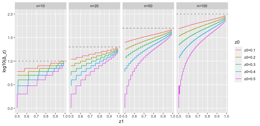
Figure 4: $\Delta_{z}$ of correlated counts under different distributional assumptions

5 Discussion

Our work provides a statistically reasoned framework for understanding privacy guarantees for PPD by extending Pufferfish to consider distributions conditioned on public information. Although we have focused on $\epsilon$-DP style privacy semantics, we could have easily considered $f$-DP (Dong et al., 2019), $\rho$-zero concentrated DP (Bun and Steinke, 2016), or other semantics which allow for an inferential testing perspective. Future work should extend the proposed approach to those frameworks.

Many view Pufferfish as harder to operationalize than DP, which some may view as a practical limitation of our work. To this, we have a few comments. First, as a reminder, we are addressing a class of problems for which DP alone does not fully describe the formal privacy loss from the data curator’s actions; comparing our work to pure DP relies on a false equivalence between the underlying problems at hand. This is an important conceptual trade-off: DP may be easier to interpret, but it can fail to capture the actions taken by data curators in these public information scenarios. Second, we consistently show throughout this paper that the tools used in DP mechanism design can be reused in our setting, and our framework provides a way to re-contextualize those guarantees and more helpfully use public information. Our work is not meant to replace DP, but to complement it. Third, and most importantly, our framework allows for more flexible semantic privacy interpretations than those offered by the usual semantic interpretations associated with DP. This offers data curators an opportunity to be more transparent about their semantic privacy guarantees in unideal but realistic privacy-preserving data processing systems. We argue this is an essential part of making data processing more transparent to end users, both for better end data utility and data curator accountability.

Note that our work is designed as a way to accommodate public information into privacy loss analysis, but this itself is not a unilateral endorsement of releasing public information to accommodate DP results. The privacy affordances offered by DP are kept closest to their idealized guarantees with no public information released outside the confines of the framework. Whenever possible, data curators should attempt to release results with randomization to satisfy DP, and carefully consider when certain cases that do not logistically accommodate this randomization occur.

Still, our proposed work is valuable because situations that necessitate public information arise frequently in the social sciences, in particular for the production of official statistics, administrative data, and survey data. The US Census Bureau’s public information use case was mandated by public law (94th Congress of the United States of America, 1975), but other cases, such as public disclosure of survey methodology (Seeman and Brummet, 2021), help more generally to quantitatively establish trust in the quality of data created by the curator. In cases like these, disclosing public information not only satisfies an important logistical requirement, but also respects a context specific normative practice on how information flows between parties. This context-specificity is an essential component in how privacy is sociologically conceived (Nissenbaum, 2009), and DP alone often fails to align with this important sociological dimension of privacy. As a result, our framework serves to align important technical and sociological goals in privacy preserving data sharing and analysis currently faced by data curators.

Acknowledgments and Disclosure of Funding

This work was supported by NSF SES-1853209. Seeman was partially supported by a U.S. Census Bureau Dissertation Fellowship. We declare no known conflicts of interest.

Appendix A Proofs

A.1 Proof of Lemma 4

Let $z\in\mathcal{Z}$ $B\in\mathcal{F}_{Y}$, $\theta_{z}\in\mathbb{D}_{\mathrm{DPz}}$, and $(s_{1},s_{2})\in\mathbb{S}_{\mathrm{pairs,DPz}}$. By Bayes rule:

$$\frac{\operatorname{\mathbb{P}}(s_{1}\mid Y\in B,\theta_{z})/\operatorname{\mathbb{P}}(s_{2}\mid Y\in B,\theta_{z})}{\operatorname{\mathbb{P}}(s_{1}\mid\theta_{z})/\operatorname{\mathbb{P}}(s_{2}\mid\theta_{z})}=\frac{\operatorname{\mathbb{P}}(Y\in B\mid s_{1},\theta_{z})}{\operatorname{\mathbb{P}}(Y\in B\mid s_{2},\theta_{z})}$$

Note that we avoid dividing by zero in either quantity because we assume $\theta_{z}\in\mathbb{D}_{\mathrm{DPz}}$ and $(s_{1},s_{2})\in\mathbb{S}_{\mathrm{pairs,DPz}}$. The ratio on the right is within $[e^{-\epsilon},e^{\epsilon}$] if and only if Equation 11 holds.

A.2 Proof of Lemma 5

Fix $z\in\mathcal{Z}$, $(s_{1},s_{2})\in\mathbb{S}_{\mathrm{pairs,DPZ}}$, and $\theta_{z}\in\mathbb{D}_{\mathrm{DPz}}$. For $B\in\mathcal{F}_{Y}$, let $B^{*}_{z}\in\mathcal{F}_{Y^{*}\times Z}$ and define $B_{z}^{*-1}\triangleq\{y\in\mathcal{Y}\mid h(y,z)=Y^{*}\}$. Then $B^{*-1}_{z}\in\mathcal{F}_{Y}$ for all $z\in\mathcal{Z}$ by measurability. This implies:

$$\operatorname{\mathbb{P}}(Y^{*}\in B^{*}_{z}\mid s_{1},\theta_{z}) =\operatorname{\mathbb{P}}(Y\in B_{z}^{*-1}\mid s_{1},\theta_{z})$$ (19)

$$\leq\operatorname{\mathbb{P}}(Y\in B_{z}^{*-1}\mid s_{2},\theta_{z})e^{\epsilon}$$ (20)

$$=\operatorname{\mathbb{P}}(Y^{*}\in B^{*}_{z}\mid s_{2},\theta_{z})e^{\epsilon}.$$ (21)

A.3 Proof of Lemma 6

Let $Y\triangleq(Y_{1},Y_{2})$ on $(\mathcal{Y},\mathcal{F}_{Y})$. By the conditional independence assumption, there exists $B_{1},B_{2}\in\mathcal{F}_{Y_{1}}\times\mathcal{F}_{Y_{2}}$ such that:

$$\operatorname{\mathbb{P}}(Y\in B\mid s_{1},\theta_{z}) =\operatorname{\mathbb{P}}(Y_{1}\in B_{1}\mid s_{1},\theta_{z})\operatorname{\mathbb{P}}(Y_{2}\in B_{2}\mid s_{1},\theta_{z})$$

$$\leq\left(e^{\epsilon_{1}}\operatorname{\mathbb{P}}(Y_{1}\in B_{1}\mid s_{2},\theta_{z})\right)\left(e^{\epsilon_{2}}\operatorname{\mathbb{P}}(Y_{2}\in B_{2}\mid s_{2},\theta_{z})\right)$$

$$=e^{(\epsilon_{1}+\epsilon_{2})}\operatorname{\mathbb{P}}(Y\in B\mid s_{2},\theta_{z}).$$

A.4 Proof of Lemma 7

First, we consider $B=2$. Let $Y\triangleq(Y_{1},Y_{2})$ on $(\mathcal{Y},\mathcal{F}_{Y})$. If $s_{1}$ and $s_{2}$ both describe entries in the same partition (either $X_{1}$ or $X_{2}$, without loss of generality), then the result is trivially satisfied. If $s_{1}$ describes an entry in $X_{1}$ and $s_{2}$ describes an entry in $X_{2}$, then:

$$\operatorname{\mathbb{P}}(Y\in B\mid s_{1},\theta_{z}) =\operatorname{\mathbb{P}}(Y_{1}\in Y_{1}^{-1}(B)\mid s_{1},\theta_{z})$$

$$\leq e^{\epsilon}\operatorname{\mathbb{P}}(Y_{1}\in Y_{1}^{-1}(B)\mid s_{2},\theta_{z})$$

$$=e^{\epsilon}\operatorname{\mathbb{P}}(Y\in B\mid s_{2},\theta_{z}).$$

Therefore in all cases, the result holds for $B=2$. By induction, this holds for any sized finite partition, i.e. $B\in\mathbb{N}$.

A.5 Proof of Lemma 8

This proof follows (Gong and Meng, 2020, Theorem 2.1) (in their setting with $k=1$ and $\gamma=1$). Without loss of generality, let $z=1$ (otherwise, replace $\mathcal{X}^{*n}$ with $\mathcal{X}^{n}\setminus\mathcal{X}^{*n}$). Specifically, for $(s_{1},s_{2})\in\mathbb{S}_{\mathrm{pairs,DPz}}$ and $B\in\mathcal{F}_{Y}$:

$$\frac{\operatorname{\mathbb{P}}(Y\in B\mid s_{1},Y\in\mathcal{X}^{n^{*}})}{\operatorname{\mathbb{P}}(Y\in B\mid s_{2},Y\in\mathcal{X}^{n^{*}})} =\frac{\operatorname{\mathbb{P}}(Y\in B\cap\mathcal{X}^{n^{*}}\mid s_{1})}{\operatorname{\mathbb{P}}(Y\in B\cap\mathcal{X}^{n^{*}}\mid s_{2})}\frac{\operatorname{\mathbb{P}}(Y\in\mathcal{X}^{n^{*}}\mid s_{2})}{\operatorname{\mathbb{P}}(Y\in\mathcal{X}^{n^{*}}\mid s_{1})}$$

$$\leq\left(e^{\epsilon}\right)\left(e^{\epsilon}\right)$$

$$\leq e^{2\epsilon}$$

A.6 Proof of Theorem 9

Let $(s_{1},s_{2})\in\mathbb{S}_{\mathrm{pairs,DPz}}$ and $B\in\mathcal{F}_{Y}$. Let $\mu_{i,\theta_{z}}\triangleq\operatorname{\mathbb{P}}(\cdot\mid\theta_{z},s_{i})$. Let $\gamma^{*}$ be the joint distribution that achieves the Wasserstein distance bound. Then:

$$\frac{\operatorname{\mathbb{P}}(Y\in B\mid s_{1},\theta_{z})}{\operatorname{\mathbb{P}}(Y\in B\mid s_{2},\theta_{z})} =\frac{\int_{\mathcal{X}}\operatorname{\mathbb{P}}(Y\in B\mid s_{1},\theta_{z},X=x)\ d\mu_{1,\theta_{z}}(x)}{\int_{\mathcal{X}}\operatorname{\mathbb{P}}(Y\in B\mid s_{2},\theta_{z},X=x)\ d\mu_{2,\theta_{z}}(x)}$$ (22)

$$=\frac{\int_{\mathcal{Y}}\int_{\mathcal{X}}\mathbbm{1}_{\{y\in B\}}\exp\left(-\frac{\epsilon L_{x}(y)}{2\sigma(\Delta_{z})}\right)\ d\mu_{1,\theta_{z}}(x)\ d\nu_{z}(y)}{\int_{\mathcal{Y}}\int_{\mathcal{X}}\mathbbm{1}_{\{y\in B\}}\exp\left(-\frac{\epsilon L_{X}(y)}{2\sigma(\Delta_{z})}\right)\ d\mu_{2,\theta_{z}}(x)\ d\nu_{z}(y)}$$ (23)

$$=\frac{\int_{\mathcal{Y}}\int_{\mathcal{X}}\int_{\mathcal{X}}\mathbbm{1}_{\{y\in B\}}\exp\left(-\frac{\epsilon L_{x}(y)}{2\sigma(\Delta_{z})}\right)\ d\gamma^{*}(x,x^{\prime})\ d\nu_{z}(y)}{\int_{\mathcal{Y}}\int_{\mathcal{X}}\int_{\mathcal{X}}\mathbbm{1}_{\{y\in B\}}\exp\left(-\frac{\epsilon L_{x^{\prime}}(y)}{2\sigma(\Delta_{z})}\right)\ d\gamma^{*}(x,x^{\prime})\ d\nu_{z}(y)}$$ (24)

Let $B_{\Delta_{z}}(x)\triangleq\{x^{\prime}\in\mathcal{X}\mid d(x,x^{\prime})\leq\Delta_{z}\}$. Then by construction and definition of the Wasserstein distance:

$$\frac{\operatorname{\mathbb{P}}(Y\in B\mid s_{1},\theta_{z})}{\operatorname{\mathbb{P}}(Y\in B\mid s_{2},\theta_{z})} =\frac{\int_{\mathcal{Y}}\int_{\mathcal{X}}\int_{B_{\Delta_{z}}(x)}\mathbbm{1}_{\{y\in B\}}\exp\left(-\frac{\epsilon L_{x}(y)}{2\sigma(\Delta_{z})}\right)\ d\gamma^{*}(x,x^{\prime})\ d\nu_{z}(y)}{\int_{\mathcal{Y}}\int_{\mathcal{X}}\int_{B_{\Delta_{z}}(x^{\prime})}\mathbbm{1}_{\{y\in B\}}\exp\left(-\frac{\epsilon L_{x^{\prime}}(y)}{2\sigma(\Delta_{z})}\right)\ d\gamma^{*}(x,x^{\prime})\ d\nu_{z}(y)}$$ (25)

$$\leq\frac{\int_{\mathcal{Y}}\int_{\mathcal{X}}\int_{B_{\Delta_{z}}(x^{\prime})}\mathbbm{1}_{\{y\in B\}}\exp\left(-\frac{\epsilon(L_{x^{\prime}}(y)+\sigma(\Delta_{z}))}{2\sigma(\Delta_{z})}\right)\ d\gamma^{*}(x,x^{\prime})\ d\nu_{z}(y)}{\int_{\mathcal{Y}}\int_{\mathcal{X}}\int_{B_{\Delta_{z}}(x^{\prime})}\mathbbm{1}_{\{y\in B\}}\exp\left(-\frac{\epsilon L_{x^{\prime}}(y)}{2\sigma(\Delta_{z})}\right)\ d\gamma^{*}(x,x^{\prime})\ d\nu_{z}(y)}$$ (26)

$$\leq\exp\left(\frac{\epsilon}{2}\right)\exp\left[\frac{\epsilon}{2}\left(\frac{\sup\left\{|L_{x}(y)-L_{x^{\prime}}(y)|\mid x,x^{\prime}\in\mathcal{X}^{n},d(x,x^{\prime})\leq\Delta_{z}\right\}}{\sigma(\Delta_{z})}\right)\right]$$ (27)

$$\leq\exp(\epsilon)$$ (28)

A.7 Proof of Theorem 10

Let $L_{X}(y)$ be the loss function from the $K$-norm gradient mechanism, and let:

$$L_{X}^{*}(y)\triangleq\frac{\left\lVert\nabla L_{X}(y)\right\rVert_{K}}{\sigma_{y}(\Delta_{Z})}$$

Then in Theorem 9 applied to $L_{X}^{*}(y)$, $\sigma(\Delta_{z})=1$. Therefore the Wasserstein $K$-norm gradient mechanism satisfies $\epsilon$-TP.

A.8 Proof of Theorem 11

Here, we fully list the assumptions needed for this theorem:

1. $n^{-1}\nabla^{2}L_{X_{n}}(y)$ exists almost everywhere $\nu_{Z_{n}}$, and the smallest eigenvalue of $L_{X_{n}}(y)$ is greater than $\alpha>0$ for all $n\in\mathbb{N}$, $y\in\mathcal{Y}$, $\nu_{Z_{n}}$ almost everywhere.

2. There exists a unique $y^{*}\in\mathcal{Y}$ such that as $n\to\infty$:

   $$Y^{*}_{n}\triangleq\operatorname*{arg\,min}_{\tilde{y}\in\mathcal{Y}}L_{X_{n}}(\tilde{y})\to_{P}y^{*}.$$

3. For all $n\in\mathbb{N}$, $\Delta_{Z_{n}}\geq\Delta^{*}>0$ w.p. 1

4. $\sigma_{y}(\Delta^{*})$ is continuous in $y$, and $\sigma_{y}(\Delta^{*})\geq\sigma^{*}(\Delta^{*})$ holds $\nu_{Z_{n}}$ almost everywhere.

5. For all $n\in\mathbb{N}$

   $$\int_{\mathcal{X}}\exp\left(-\frac{\alpha\left\lVert y_{n}-y_{n}^{*}\right\rVert_{K}}{2\sigma_{y_{n}^{*}}(\Delta^{*})}\right)d\nu_{Z_{n}}<\infty.$$

6. $Z_{n}\to_{D}Z^{*}$ and $\nu_{Z_{n}}\to_{D}\nu_{Z^{*}}\ll\lambda$.

7. Let $B_{\delta}(\cdot)$ be a $K$-norm ball of radius $\delta$. We assume that for $a\in\mathcal{Y}$ and some $\delta>0$:

   $$\int_{B_{\delta}(y_{n}^{*})}d\nu_{Z_{n}}(a)=\Omega_{P}(1)$$

   In words, the base measure should support the true solution $y^{*}$ with probability bounded away from zero by some constant.

Let $f_{n}(y)$ be the density of the Wasserstein $K$-norm gradient mechanism:

$$f_{n}(y_{n})\propto\exp\left(-\frac{\epsilon\left\lVert\nabla L_{X_{n}}(y_{n})\right\rVert_{K}}{2\sigma_{y}(\Delta_{Z_{n}})}\right)d\nu_{Z_{n}}(y_{n}),$$

Let $a_{n}\triangleq n(y_{n}-y_{n}^{*})$ with density $h_{n}(\cdot)$ so that:

$$h_{n}(a_{n})\propto\exp\left(-\frac{\epsilon\left\lVert\nabla L_{X_{n}}(y_{n}^{*}+a_{n}/n)\right\rVert_{K}}{2\sigma_{y}(\Delta_{Z_{n}})}\right)d\nu_{Z_{n}}(y_{n}^{*}+a_{n}/n).$$

Note that in the transformation above, the Jacobian constant $n^{-1}$ gets absorbed in the proportionality. Next, we Taylor expand the loss function:

$$\nabla L_{X_{n}}(y_{n})=\nabla L_{X_{n}}\left(y_{n}^{*}+a_{n}/n\right)=\nabla^{2}L_{X_{n}}(y^{*}_{n})\frac{a_{n}}{n}+o_{p}(1)$$ (29)

Following the proof of (Reimherr and Awan, 2019, Theorem 3.2), using Assumptions (1) - (4), there exists a constant $C>0$ such that:

$$-\frac{1}{\sigma_{y^{*}_{n}+a_{n}/n}(\Delta_{Z_{n}})}\left\lVert\nabla L_{n}(y^{*}_{n}+a_{n}/n)\right\rVert_{K}\leq-\frac{C\alpha}{\sigma^{*}(\Delta^{*})}\left\lVert a_{n}\right\rVert_{2}.$$

Then by the dominated convergence theorem, Assumptions (5) - (6), and the continuity of $\sigma$, we conclude that:

$$\lim_{n\to\infty}h_{n}(a_{n})=h(a)\propto\exp\left(-\frac{\epsilon}{2\sigma_{y^{*}}(\Delta^{*})}\left\lVert\Sigma^{-1}a\right\rVert_{K}\right),$$ (30)

with respect to the base measure $\nu_{Z^{*}}(a)$ (note that Assumption (6) ensures the asymptotic base measure supports $y^{*}$). This is a $K$-norm density with respect to the asymptotic base measure $\nu_{Z^{*}}$. Therefore, $Y_{n}$ concentrates around $Y_{n}^{*}$ at a rate at least as fast as for the standard $K$-norm gradient mechanism, i.e., $a_{n}=O_{p}(1)$, yielding the desired result.

A.9 Proof of Lemma 12

Fix $\delta>0$, $\bm{x}\in\mathcal{X}$, and let $d_{H}$ be a metric on $\mathcal{X}$. Then for sufficiently large $m$:

$$\sup_{\theta_{z}\in\Theta_{Z}}\sup_{(s_{1},s_{2})\in\mathbb{S}_{\mathrm{pairs,DPz}}}W_{\infty}\{\operatorname{\mathbb{P}}(\cdot,\mid\theta_{z},s_{1}),\operatorname{\mathbb{P}}(\cdot,\mid\theta_{z},s_{2})\}$$

$$\geq\sup_{(s_{1},s_{2})\in\mathbb{S}_{\mathrm{pairs,DPz}}}W_{\infty}\{\operatorname{\mathbb{P}}(\cdot,\mid\theta_{z,\bm{x}}^{(m)},s_{1}),\operatorname{\mathbb{P}}(\cdot,\mid\theta_{z,\bm{x}}^{(m)},s_{2})\}$$

$$\geq 1-\delta$$

Since this is true for arbitrary $\delta$, then we can ensure $\Delta_{z}\geq 1$, yielding the desired result.

A.10 Proof of Theorem 15

First we show that $Y$ has a monotone likelihood in $\theta$. Let $\Xi\triangleq Y-T(X)$. Then the marginal density of $Y$, $m_{\theta}(y)$ can be expressed as a function of the density of $\Xi$, $g_{\Xi}(\xi)$ as a convolution:

$$g_{\Xi}(\xi)\propto\exp\left(-\frac{\epsilon}{2\sigma(\Delta_{z})}L(\xi)\right)\implies m_{\theta}(y)\triangleq\int_{\mathcal{X}}g_{\Xi}(y-x)f_{\theta}(x)\ dx.$$

Let $y_{1},y_{2}\in\mathcal{Y}$ such that $y_{1}<y_{2}$ and $\theta_{1},\theta_{2}\in\Theta$ such that $\theta_{1}<\theta_{2}$. Suppose first that $n=1$. Note that $f_{\theta}(x)$ has a monotone likelihood because $f_{\theta}$ belongs to an exponential family. Similarly, $g_{\Xi}$ has a monotone likelihood ratio by construction. Then using the main result from (Wijsman, 1985):

$$\int_{\mathcal{X}}g_{\Xi}(y_{1}-x)f_{\theta_{1}}(x)\ dx\int_{\mathcal{X}}g_{\Xi}(y_{2}-x)f_{\theta_{2}}(x)\ dx\geq\int_{\mathcal{X}}g_{\Xi}(y_{2}-x)f_{\theta_{1}}(x)\ dx\int_{\mathcal{X}}g_{\Xi}(y_{2}-x)f_{\theta_{1}}(x)\ dx$$

$$\implies m_{\theta_{1}}(y_{1})m_{\theta_{2}}(y_{2})\geq m_{\theta_{2}}(y_{1})m_{\theta_{1}}(y_{2})$$

$$\implies\frac{m_{\theta_{2}}(y_{1})}{m_{\theta_{1}}(y_{1})}\leq\frac{m_{\theta_{2}}(y_{2})}{m_{\theta_{1}}(y_{2})}$$

The results extends to arbitrary $n$ by the iid assumption, and therefore $Y$ has a monotone likelihood ratio in $\theta$.

Next, let $\phi:\mathcal{Y}^{*}\mapsto[0,1]$ be an unbiased test for $H_{0}:\theta\leq\theta_{0}$ versus $H_{1}:\theta>\theta_{0}$. Fix the type I error as $\alpha$. Using the fact that $Y$ has a monotone likelihood ratio in $\theta$ and the unbiasedness of $\phi$, we know $\beta_{\phi}(\theta_{0})\leq\beta_{\phi}(\theta_{1})$ for all $\theta_{0},\theta_{1}\in\Theta$ such that $\theta_{0}\leq\theta_{1}$, where:

$$\beta_{Y^{*}}(\theta)\triangleq\operatorname{\mathbb{E}}_{\theta}[\phi(Y^{*})]=\operatorname{\mathbb{E}}_{\theta}[\phi(Y^{*})(\mathbbm{1}_{\{Y=Y^{*}\}}+\mathbbm{1}_{\{Y<Y^{*}\}}+\mathbbm{1}_{\{Y>Y^{*}\}})].$$

When $\theta=\theta_{0}$ and $Y<Y^{*}$, using the MLR property, there exists a test $\phi^{\prime}:\mathcal{Y}\times\mathcal{Z}\mapsto[0,1]$ such that $\phi^{\prime}(Y,Z)=\phi(Y^{*})$ whenever $Y=Y^{*}$, and:

$$\operatorname{\mathbb{E}}_{\theta_{0}}[\phi^{\prime}(Y,Z)\mid Y<Y^{*}]\leq\operatorname{\mathbb{E}}_{\theta_{0}}[\phi(Y^{*})\mid Y<Y^{*}]$$

Let $\gamma\triangleq\operatorname{\mathbb{E}}_{\theta_{0}}[\phi(Y^{*})-\phi^{\prime}(Y,Z)]\in[0,\alpha]$. We can modify $\phi^{\prime}$ such that, for $Y>Y^{*}$:

$$\operatorname{\mathbb{E}}_{\theta_{0}}[\phi^{\prime}(Y,Z)-\phi(Y^{*})\mid Y>Y^{*}]=\gamma$$

This yields a final test $\phi^{\prime}(Y,Z)$ which dominates $\phi(Y^{*})$ and is still level $\alpha$. As long as $\operatorname{\mathbb{P}}_{\theta}(Y\neq Y^{*})>0$, the dominance is non-trivial; the new test may have a smaller type I error, type II error, or both.

A.11 Proof of Theorem 16

Throughout this proof, we take $\pi$ to refer to the density of the variables in question. The target density has the form:

$$\pi(\theta\mid y,z) =\frac{\pi(\theta,y\mid z)}{\pi(y\mid z)}$$

$$=\frac{\int\pi(\theta,x,y\mid z)\ d\nu_{X}}{\int\pi(y,x\mid z)\ d\nu_{X}}$$

$$=\frac{\int\pi(\theta\mid z)\pi(x\mid\theta,z)\pi(y\mid x,z)\ d\nu_{X}}{\int\int\pi(\theta\mid z)\pi(x\mid\theta,z)\pi(y\mid x,z)\ d\nu_{X}\ d\nu_{\Theta}}$$

Following (Gong, 2019), let $A$ be a Bernoulli variable with success probability associated with accepting one proposal in the algorithm with public information $z$ and proposed samples $\theta^{*}\in\Theta$ and $x^{*}\in\mathcal{X}^{n}$. Define:

$$C\triangleq\sup_{y^{*}\in\mathcal{Y}}\pi(y^{*}\mid x^{*},z)$$

Then:

$$\pi(\theta^{*}\mid A=1,z) =\int\frac{\pi(\theta^{*},x^{*},A=1)\ d\nu_{X}}{\pi(A=1)}$$

$$=\frac{C\int\pi(\theta\mid z)\pi(x\mid\theta,z)\pi(y\mid x,z)\ d\nu_{X}}{C\int\int\pi(\theta\mid z)\pi(x\mid\theta,z)\pi(y\mid x,z)\ d\nu_{X}\ d\nu_{\Theta}}$$

$$=\pi(\theta\mid y,z)$$

Therefore accepted samples in Algorithm 1 are exact draws from $\theta\mid Y,Z$.

Appendix B Complete Algorithms

Result: One sample from $\theta\mid Y,Z$

Sample $\theta^{*}\sim\pi(\theta\mid Z)$ ;

Sample $X^{*}\sim\pi(\cdot\mid\theta^{*},Z)$ ;

Sample $U\sim\mathrm{Unif}(0,1)$ ;

if 

$$\frac{\pi(Y\mid X^{*},Z)}{\sup_{y^{*}\in\mathcal{Y}}\pi(y^{*}\mid X^{*},Z)}\leq U$$

 then

       Return $\theta^{*}$.

else

       Go to beginning.

end if

Algorithm 1 Posterior rejection sampling conditional on public information

Result: Estimate of $\widehat{\operatorname{\mathbb{E}}}[a(\theta)\mid Y,Z]$ using proposals from density $g$

Sample $\theta^{(1)},\cdots,\theta^{(m)}\sim\pi(\theta\mid Z=z)$ ;

Sample $X^{(j)}\sim\pi(\cdot\mid\Theta=\theta^{(j)},Z=z)$ ;

Calculate:

$$w^{(j)}=\frac{\pi(Y\mid X^{(j)},Z)\pi(\theta^{(j)}\mid Z)}{g(\theta^{(j)})}$$

Return:

$$\widehat{\operatorname{\mathbb{E}}}[a(\theta)\mid Y,Z]\triangleq\frac{\sum_{j=1}^{m}w^{(j)}a(\theta^{(j)})}{\sum_{j=1}^{m}w^{(j)}}$$

Algorithm 2 Posterior importance sampling conditional on public information

Appendix C Complete Example Derivations

Example 3 (Derivation of Example 1)

Suppose we have the setup as given in Equations 14 and 15. First, let’s consider the case where $Z\mathchoice{\mathrel{\hbox to0.0pt{$\displaystyle\perp$\hss}\mkern 2.0mu{\displaystyle\perp}}}{\mathrel{\hbox to0.0pt{$\textstyle\perp$\hss}\mkern 2.0mu{\textstyle\perp}}}{\mathrel{\hbox to0.0pt{$\scriptstyle\perp$\hss}\mkern 2.0mu{\scriptstyle\perp}}}{\mathrel{\hbox to0.0pt{$\scriptscriptstyle\perp$\hss}\mkern 2.0mu{\scriptscriptstyle\perp}}}X_{1},\overline{X}$, in which case we need only consider:

$$\begin{pmatrix}\overline{X}\\ X_{1}\end{pmatrix}\sim N\left(\begin{pmatrix}\mu\\ \mu\end{pmatrix},\begin{pmatrix}\sigma^{2}/n&\sigma^{2}/n\\ \sigma^{2}/n&\sigma^{2}\end{pmatrix}\right)\implies\overline{X}\mid X_{1}=v\sim N\left(\mu+\frac{1}{n}(v-\mu),\frac{n-1}{n^{2}}\sigma^{2}\right)$$ (31)

Define $\operatorname{\mathbb{P}}_{\theta,v_{1}}(B)\triangleq\operatorname{\mathbb{P}}_{\theta}(\overline{X}\in B\mid X_{1}=v_{1})$. By definition:

$$W_{\infty}\left(\operatorname{\mathbb{P}}_{\theta,v_{1}},\operatorname{\mathbb{P}}_{\theta,v_{2}}\right)\triangleq\inf_{\gamma\in\Gamma(\operatorname{\mathbb{P}}_{\theta,v_{1}},\operatorname{\mathbb{P}}_{\theta,v_{2}})}\operatorname*{ess\,sup}_{(y_{1},y_{2})\in\Omega_{\gamma}}|y_{1}-y_{2}|.$$

The solution to the optimization problem is explicitly calculable. If $V_{1}\sim\operatorname{\mathbb{P}}_{\theta,v_{1}}$ and $V_{2}\sim\operatorname{\mathbb{P}}_{\theta,v_{2}}$, then the optimal transport solution takes the joint distribution where, w.p. 1:

$$V_{2}=V_{1}+\frac{v_{2}-v_{1}}{n}.$$ (32)

To give some intuition for Equation 32, if we fix $\theta$, then $\{\operatorname{\mathbb{P}}_{\theta,v}\mid v\in\mathbb{R}\}$ is a location family with a location parameter linear in $v$. Therefore in the $W_{\infty}$ optimal transport solution, each infinitesimal piece of probability mass travels the same constant distance as specified by the difference in conditional means.Any other solution would necessarily require a larger essential supremum.

The optimal transport solution in Equation 32 is independent of both $\mu$ and $\sigma$, and therefore only depends on the secret pairs $(s_{1},s_{2})\in\mathbb{S}_{\mathrm{pairs}}$ for which:

$$\sup_{\theta\in\mathbb{D}}\sup_{(s_{1},s_{2})\in\mathbb{S}_{\mathrm{pairs}}}W_{\infty}(\operatorname{\mathbb{P}}_{\theta,v_{1}},\operatorname{\mathbb{P}}_{\theta,v_{2}})=\frac{\Delta}{n}$$

This allows us to instantiate the Wasserstein exponential mechanism. First, for all databases whose $L_{1}$ distance is bounded by $\Delta/n$ we have:

$$\sup_{X,X^{\prime}\colon\left\lVert X-X^{\prime}\right\rVert_{L_{1}}\leq\Delta/n}|L_{X}(y)-L_{X^{\prime}}(y)|\leq\Delta/n$$ (33)

Therefore the Wasserstein exponential mechanism gives us exactly the same result as the $\epsilon$-DP exponential mechanism in Equation 13 without additional public information.

Next, we introduce $Z$. Performing a similar analysis using Equation 15 gives us:

$$\overline{X}\mid X_{1}=v,Z=z\sim N\left(\mu+\Sigma_{XVZ}^{T}\Sigma_{VZ}^{-1}\begin{pmatrix}v-\mu\\ z-\mu_{Z}\end{pmatrix},\frac{\sigma^{2}}{n}-\Sigma_{XVZ}^{T}\Sigma_{VZ}^{-1}\Sigma_{XVZ}\right).$$ (34)

Again, by properties of the conditional multivariate normal, the resulting family is still a location family parameterized by a (more complicated) linear change in $v$. However, this indicates that the dependence affects the Wasserstein distance through the nuisance parameter $\sigma^{2}$, which canceled in the previous case:

$$\sup_{\theta\in\mathbb{D}}\sup_{(s_{1},s_{2})\in\mathbb{S}_{\mathrm{pairs}}}W_{\infty}(\operatorname{\mathbb{P}}_{\theta,v_{1}},\operatorname{\mathbb{P}}_{\theta,v_{2}})=\sup_{\theta\in\mathbb{D}}\left[\Sigma_{XVZ}^{T}\Sigma_{VZ}^{-1}\begin{pmatrix}\Delta\\ z-\mu_{Z}\end{pmatrix}\right].$$

Therefore in this situation, the “sensitivity” of the Wasserstein exponential mechanism loss depends explicitly on what kinds of dependence we allow between the private and public information, i.e. how we choose $\mathbb{D}$.

Example 4 (Count Data Satisfying $\epsilon$-TP and SDL measures)

Let $X\in\{0,1\}^{n}$, and our goal is to implement the Wassserstein exponential mechanism targeting $S_{n}\triangleq\sum_{i=1}^{n}X_{i}$ with $L_{X}(y)=|y-S_{n}|$. The secret pairs are of the form:

$$s_{ij}=\{\omega\in\Omega\mid X_{i}(\omega)=j\},\quad\mathbb{S}_{\mathrm{pairs}}\triangleq\left\{(s_{i0},s_{i1})\mid i\in[n]\right\}.$$

Possible distributions conditioned on the secrets take the form:

$$\operatorname{\mathbb{P}}\left(S_{n}=k\mid s_{i0},Z=z\right)=f_{\theta_{z},0}(k),\quad\operatorname{\mathbb{P}}\left(S_{n}=k\mid s_{i1},Z=z\right)=f_{\theta_{z},1}(k).$$

Therefore, we need to consider:

$$\Delta_{z}=\sup_{\theta_{z}\in\Theta_{z}}W_{\infty}\left(\operatorname{\mathbb{P}}_{\theta_{z},0},\operatorname{\mathbb{P}}_{\theta_{z},1}\right)=\sup_{\theta_{z}\in\Theta_{z}}\sup_{t\in\mathcal{T}}|F^{-}_{\theta_{z},0}(t)-F^{-}_{\theta_{z},1}(t)|\in\{1,\dots,n\},$$ (35)

where

$$\mathcal{T}=\left\{\operatorname{\mathbb{P}}\left(S_{n}\leq k\mid s_{j0},Z=z\right)\mid j\in\{1,\dots n\}\right\}.$$

We consider public information $Z$ to be the property that releasing $(S_{n},n-S_{n})$ satisfies different Statistical Disclosure Limitation (SDL) measures, namely $k$-anonymity (Sweeney, 2002) and $L_{1}$-distance $t$-closeness (Li et al., 2007) to a public statistic $t^{*}$:

$$\begin{cases}S_{n}\text{ satisfies $k$-anonymity}\implies S_{n}\in\{k,k+1,\dots,n-k\}\\ S_{n}\text{ satisfies $L_{1}$-$t$-closeness}\implies\left|\frac{S_{n}}{n}-t^{*}\right|\leq t.\end{cases}$$ (36)

Because both of these are descriptors of the secret pairs, we can jointly satisfy some SDL measures as well as $\epsilon$-DP. However, this comes at the expense of the guarantees holding for fewer secret pairs.

Example 2 demonstrates how $\epsilon$-TP changes the unit of privacy analysis in the presence of $Z$. While SDL methods typically consider an equivalence class of databases with the same SDL properties, and DP methods typically consider an entire database schema, our $\epsilon$-TP considers a partial database schema. This means $\epsilon$-TP only confers protections for those databases which plausibly agree with $Z$, but this partial schema could be constrained by the practical privacy guarantees afforded by SDL.

References

- 94th Congress of the United States of America (1975) 94th Congress of the United States of America. PL 94-171: Redistricting Data, 1975.
- Abowd et al. (2019a) John Abowd, Robert Ashmead, Garfinkel Simson, Daniel Kifer, Philip Leclerc, Ashwin Machanavajjhala, and William Sexton. Census topdown: Differentially private data, incremental schemas, and consistency with public knowledge. US Census Bureau, 2019a.
- Abowd et al. (2019b) John Abowd, Daniel Kifer, Brett Moran, Robert Ashmead, and William Sexton. Census TopDown Algorithm: Differentially Private Data, Incremental Schemas, and Consistency with Public Knowledge. 2019b.
- Ashmead et al. (2019) Robert Ashmead, Daniel Kifer, Philip Leclerc, Ashwin Machanavajjhala, and William Sexton. Effective Privacy After Adjusting for Invariants with Appli-cations to the 2020 Census. Technical report, Technical Report. US Census Bureau, 2019.
- Asi and Duchi (2020) Hilal Asi and John C Duchi. Instance-optimality in differential privacy via approximate inverse sensitivity mechanisms. In H Larochelle, M Ranzato, R Hadsell, M F Balcan, and H Lin, editors, Advances in Neural Information Processing Systems, volume 33, pages 14106–14117. Curran Associates, Inc., 2020. URL https://proceedings.neurips.cc/paper/2020/file/a267f936e54d7c10a2bb70dbe6ad7a89-Paper.pdf.
- Awan and Rao (2021) Jordan Awan and Vinayak Rao. Privacy-Aware Rejection Sampling. arXiv preprint arXiv:2108.00965, 2021.
- Awan and Slavković (2018) Jordan Awan and Aleksandra Slavković. Differentially private uniformly most powerful tests for binomial data. Advances in Neural Information Processing Systems, 31:4208–4218, 2018.
- Barak et al. (2007) Boaz Barak, Kamalika Chaudhuri, Cynthia Dwork, Satyen Kale, Frank McSherry, and Kunal Talwar. Privacy, accuracy, and consistency too: a holistic solution to contingency table release. In Proceedings of the twenty-sixth ACM SIGMOD-SIGACT-SIGART symposium on Principles of database systems, pages 273–282, 2007.
- Bassily et al. (2013) Raef Bassily, Adam Groce, Jonathan Katz, and Adam Smith. Coupled-worlds privacy: Exploiting adversarial uncertainty in statistical data privacy. In 2013 IEEE 54th Annual Symposium on Foundations of Computer Science, pages 439–448. IEEE, 2013.
- Bassily et al. (2020) Raef Bassily, Albert Cheu, Shay Moran, Aleksandar Nikolov, Jonathan Ullman, and Steven Wu. Private Query Release Assisted by Public Data. In Hal Daumé III and Aarti Singh, editors, Proceedings of the 37th International Conference on Machine Learning, volume 119 of Proceedings of Machine Learning Research, pages 695–703. PMLR, 2020. URL https://proceedings.mlr.press/v119/bassily20a.html.
- Biswas et al. (2020) Sourav Biswas, Yihe Dong, Gautam Kamath, and Jonathan Ullman. CoinPress: Practical Private Mean and Covariance Estimation. Advances in Neural Information Processing Systems, 33, 2020.
- Blackwell (1953) David Blackwell. Equivalent comparisons of experiments. The annals of mathematical statistics, pages 265–272, 1953.
- Bun and Steinke (2016) Mark Bun and Thomas Steinke. Concentrated differential privacy: Simplifications, extensions, and lower bounds. In Theory of Cryptography Conference, pages 635–658. Springer, 2016.
- Canonne et al. (2019) Clément L Canonne, Gautam Kamath, Audra McMillan, Adam Smith, and Jonathan Ullman. The structure of optimal private tests for simple hypotheses. In Proceedings of the 51st Annual ACM SIGACT Symposium on Theory of Computing, pages 310–321, 2019.
- Desfontaines and Pejó (2019) Damien Desfontaines and Balázs Pejó. Sok: differential privacies. arXiv preprint arXiv:1906.01337, 2019.
- Ding et al. (2011) Bolin Ding, Marianne Winslett, Jiawei Han, and Zhenhui Li. Differentially private data cubes: optimizing noise sources and consistency. In Proceedings of the 2011 ACM SIGMOD International Conference on Management of data, pages 217–228, 2011.
- Dong et al. (2019) Jinshuo Dong, Aaron Roth, and Weijie J Su. Gaussian differential privacy. arXiv preprint arXiv:1905.02383, 2019.
- Dwork et al. (2006a) Cynthia Dwork, Krishnaram Kenthapadi, Frank McSherry, Ilya Mironov, and Moni Naor. Our data, ourselves: Privacy via distributed noise generation. In Annual International Conference on the Theory and Applications of Cryptographic Techniques, pages 486–503. Springer, 2006a.
- Dwork et al. (2006b) Cynthia Dwork, Frank McSherry, Kobbi Nissim, and Adam Smith. Calibrating noise to sensitivity in private data analysis. In Theory of cryptography conference, pages 265–284. Springer, 2006b.
- Dwork et al. (2014) Cynthia Dwork, Aaron Roth, and others. The algorithmic foundations of differential privacy. Foundations and Trends in Theoretical Computer Science, 9(3-4):211–407, 2014.
- Dwork et al. (2017) Cynthia Dwork, Adam Smith, Thomas Steinke, and Jonathan Ullman. Exposed! a survey of attacks on private data. Annual Review of Statistics and Its Application, 4:61–84, 2017.
- Fearnhead and Prangle (2012) Paul Fearnhead and Dennis Prangle. Constructing summary statistics for approximate Bayesian computation : semi-automatic approximate Bayesian computation. Journal of the Royal Statistical Society. Series B (Statistical Methodology), 74(3):419–474, 2012.
- Foulds et al. (2016) James Foulds, Joseph Geumlek, Max Welling, and Kamalika Chaudhuri. On the theory and practice of privacy-preserving Bayesian data analysis. arXiv preprint arXiv:1603.07294, 2016.
- Gao et al. (2021) Jie Gao, Ruobin Gong, and Fang-Yi Yu. Subspace Differential Privacy. arXiv preprint arXiv:2108.11527, 2021.
- Ghosh et al. (2012) Arpita Ghosh, Tim Roughgarden, and Mukund Sundararajan. Universally Utility-Maximizing Privacy Mechanisms. SIAM Journal on Computing, 41(6):1673–1693, 2012.
- Gong (2019) Ruobin Gong. Exact inference with approximate computation for differentially private data via perturbations. arXiv preprint arXiv:1909.12237, 2019.
- Gong (2020) Ruobin Gong. Transparent privacy is principled privacy. arXiv preprint arXiv:2006.08522, 2020.
- Gong and Meng (2020) Ruobin Gong and Xiao-Li Meng. Congenial Differential Privacy under Mandated Disclosure. In Proceedings of the 2020 ACM-IMS on Foundations of Data Science Conference, pages 59–70, 2020.
- Hay et al. (2010) Michael Hay, Vibhor Rastogi, Gerome Miklau, and Dan Suciu. Boosting the accuracy of differentially private histograms through consistency. Proceedings of the VLDB Endowment, 3(1-2):1021–1032, 2010.
- He et al. (2014) Xi He, Ashwin Machanavajjhala, and Bolin Ding. Blowfish Privacy: Tuning Privacy-Utility Trade-Offs Using Policies. In Proceedings of the 2014 ACM SIGMOD International Conference on Management of Data, SIGMOD ’14, page 1447–1458, New York, NY, USA, 2014. Association for Computing Machinery. ISBN 9781450323765. doi: 10.1145/2588555.2588581. URL https://doi.org/10.1145/2588555.2588581.
- Kasiviswanathan and Smith (2014) Shiva P Kasiviswanathan and Adam Smith. On the’semantics’ of differential privacy: A bayesian formulation. Journal of Privacy and Confidentiality, 6(1), 2014.
- Kasiviswanathan and Smith (2008) Shiva Prasad Kasiviswanathan and Adam Smith. A note on differential privacy: Defining resistance to arbitrary side information. CoRR abs/0803.3946, 2008.
- Kifer and Machanavajjhala (2011) Daniel Kifer and Ashwin Machanavajjhala. No free lunch in data privacy. In Proceedings of the 2011 ACM SIGMOD International Conference on Management of data, pages 193–204, 2011.
- Kifer and Machanavajjhala (2014) Daniel Kifer and Ashwin Machanavajjhala. Pufferfish: A framework for mathematical privacy definitions. ACM Transactions on Database Systems (TODS), 39(1):1–36, 2014.
- Li et al. (2007) Ninghui Li, Tiancheng Li, and Suresh Venkatasubramanian. t-closeness: Privacy beyond k-anonymity and l-diversity. In 2007 IEEE 23rd International Conference on Data Engineering, pages 106–115. IEEE, 2007.
- Liu et al. (2016) Changchang Liu, Supriyo Chakraborty, and Prateek Mittal. Dependence Makes You Vulnberable: Differential Privacy Under Dependent Tuples. 2016.
- McKenna et al. (2018) Ryan McKenna, Gerome Miklau, Michael Hay, and Ashwin Machanavajjhala. Optimizing error of high-dimensional statistical queries under differential privacy. Proceedings of the VLDB Endowment, 11(10):1206–1219, 2018.
- McSherry and Talwar (2007) Frank McSherry and Kunal Talwar. Mechanism design via differential privacy. In 48th Annual IEEE Symposium on Foundations of Computer Science (FOCS’07), pages 94–103. IEEE, 2007.
- Nissenbaum (2009) Helen Nissenbaum. Privacy in context. Stanford University Press, 2009.
- Pennsylvania Department of Health (2022) Pennsylvania Department of Health. COVID-19 in Pennsylvania, 2022. URL https://www.health.pa.gov/topics/disease/coronavirus/Pages/Coronavirus.aspx.
- Quick (2021) Harrison Quick. Generating Poisson-distributed differentially private synthetic data. Journal of the Royal Statistical Society: Series A (Statistics in Society), 184(3):1093–1108, 2021.
- Reimherr and Awan (2019) Matthew Reimherr and Jordan Awan. KNG: The k-norm gradient mechanism. Advances in Neural Information Processing Systems, 32, 2019.
- Ruggles et al. (2022) Steven Ruggles, Sarah Flood, Sophia Foster, Ronald Goeken, Jose Pacas, Megan Schouweiler, and Matthew Sobek. IPUMS USA: Version 10.0 [dataset], 2022. URL https://www.ipums.org/.
- Santos-Lozada et al. (2020) Alexis R Santos-Lozada, Jeffrey T Howard, and Ashton M Verdery. How differential privacy will affect our understanding of health disparities in the United States. Proceedings of the National Academy of Sciences, 117(24):13405–13412, 2020.
- Seeman and Brummet (2021) Jeremy Seeman and Quentin Brummet. Posterior Risk and Utility from Private Synthetic Weighted Survey Data. In Presented at World Meeting of the International Society for Bayesian Analysis (ISBA), 2021.
- Seeman et al. (2020) Jeremy Seeman, Aleksandra Slavković, and Matthew Reimherr. Private Posterior Inference Consistent with Public Information: a Case Study in Small Area Estimation from Synthetic Census Data. Privacy in Statistical Databases, 2020.
- Seeman et al. (2021) Jeremy Seeman, Matthew Reimherr, and Aleksandra Slavković. Exact Privacy Guarantees for Markov Chain Implementations of the Exponential Mechanism with Artificial Atoms. Advances in Neural Information Processing Systemsa, 2021.
- Slavkovic and Seeman (2022) Aleksandra Slavkovic and Jeremy Seeman. Statistical Data Privacy: A Song of Privacy and Utility, 2022. URL https://arxiv.org/abs/2205.03336.
- Slavković and Lee (2010) Aleksandra B Slavković and Juyoun Lee. Synthetic two-way contingency tables that preserve conditional frequencies. Statistical Methodology, 7(3):225–239, 2010.
- Snoke and Slavković (2018) Joshua Snoke and Aleksandra Slavković. pMSE mechanism: differentially private synthetic data with maximal distributional similarity. In International Conference on Privacy in Statistical Databases, pages 138–159. Springer, 2018.
- Song et al. (2017) Shuang Song, Yizhen Wang, and Kamalika Chaudhuri. Pufferfish privacy mechanisms for correlated data. In Proceedings of the 2017 ACM International Conference on Management of Data, pages 1291–1306, 2017.
- Soto and Reimherr (2021) Carlos Soto and Matthew Reimherr. Differential Privacy over Riemannian Manifolds. Advances in Neural Information Processing Systems, 2021.
- Sweeney (2002) Latanya Sweeney. k-anonymity: A model for protecting privacy. International Journal of Uncertainty, Fuzziness and Knowledge-Based Systems, 10(05):557–570, 2002.
- Torkzadehmahani et al. (2019) Reihaneh Torkzadehmahani, Peter Kairouz, and Benedict Paten. Dp-cgan: Differentially private synthetic data and label generation. In Proceedings of the IEEE/CVF Conference on Computer Vision and Pattern Recognition Workshops, page 0, 2019.
- Wijsman (1985) Robert A Wijsman. A useful inequality on ratios of integrals, with application to maximum likelihood estimation. Journal of the American Statistical Association, 80(390):472–475, 1985.
- Xiao et al. (2021) Yingtai Xiao, Zeyu Ding, Yuxin Wang, Danfeng Zhang, and Daniel Kifer. Optimizing fitness-for-use of differentially private linear queries. Proceedings of the VLDB Endowment, 14(10), 2021.
- Zhang et al. (2020) Wanrong Zhang, Olga Ohrimenko, and Rachel Cummings. Attribute Privacy: Framework and Mechanisms, 2020. URL https://arxiv.org/abs/2009.04013.