Convergence of the Planewave Approximations for Quantum Incommensurate Systems

Abstract

Incommensurate structures arise from stacking single layers of low-dimensional materials on top of one another with misalignment such as an in-plane twist in orientation. While these structures are of significant physical interest, they pose many theoretical challenges due to the loss of periodicity. In this paper, we characterize the density of states of Schrödinger operators in the weak sense for the incommensurate system and develop novel numerical methods to approximate them. In particular, we (i) justify the thermodynamic limit of the density of states in the real space formulation; and (ii) propose efficient numerical schemes to evaluate the density of states based on planewave approximations and reciprocal space sampling. We present both rigorous analysis and numerical simulations to support the reliability and efficiency of our numerical algorithms.

1 Introduction

Low dimensional materials have attracted extraordinary level of interest in the materials science and physics communities due to the unique electronic, optical, and mechanical properties [2, 16, 39]. In particular, when two layers of 2D materials are stacked on top of each other with a small misalignment (such as a twist), they produce incommensurate moiré patterns. In the small twist case for example, the electronic properties develop fundamental twist-dependent electronic behaviors such as Van Hove singularities and superconductivity at the magic angle (see e.g. [5, 6, 7, 10, 11, 38]). It is of great importance to study these structures from a theoretical and computational point of view and learn how to control the desired properties by choice of system parameters such as material type and twist angles.

The conventional method for simulating the incommensurate systems is to construct a supercell approximation with artificial strain [22, 23, 25], which then allows for the use of Bloch theory and conventional band-structure methods. However, these approaches are usually computationally expensive, as one may need extremely large supercells to achieve the required accuracy. Further, these methods often require restricting choice of twist angle or including unphysical strains in the system.

The purpose of this work is to study the density of states (DoS) of a linear Schrödinger operator for incommensurate systems from the mathematical point of view. We limit our focus to operators over $\mathbb{R}^{2}$, but in future works will include the out-of-plane dimension and address choice of potentials. The DoS characterizes the spectrum distribution of the system Hamiltonian, and is an observable of interest in the study of 2D materials.

The first issue is that a definition of the DoS of the Schrödinger operator for incommensurate systems is missing. In [30], the DoS was introduced in the weak sense within the tight-binding models, which can not be directly generalized to continuous models. Although the linear Schrödinger operator has a simple form, the lack of compactness, broken translation symmetry, and continuous nature of the operator make it difficult to address the DoS of an incommensurate system. To derive an explicit formulation of the “weak” DoS, we resort to the theory of pseudodifferential operators, which entails information in specific functions, the so-called symbols, containing the position $x$ and momentum $\xi$ variables simultaneously [12, 17, 33, 41]. This theory provides a powerful tool to describe an operator algebraically by various functions. By using the language of pseudodifferential operators, specifically the symbolic calculus, we are able to justify the “weak” DoS of the incommensurate system as a thermodynamic limit by exploiting the ergodicity of the incommensurate system.

The second problem is how to efficiently evaluate the (well-defined) DoS of an incommensurate system. In [40], a planewave method was proposed to discretize the wavefunction and Hamiltonian with a brute energy cutoff, which essentially transfers the low dimensional incommensurate problem into a high dimensional periodic problem. This approach gives rise to a discrete problem that is expensive most of the time and converges slowly with respect to the energy cutoff. Moreover, there was no theoretical analysis. The current paper develops a novel planewave discretization method with an energy cutoff scheme that is designed specifically for the incommensurate problems, and provides a rigorous analysis for the reliability and efficiency of the method. In particular, we split the cutoff of wave vectors in the high dimensional reciprocal space into two directions: one direction increases the planewave frequency while the other one traverses the reciprocal space. A key observation is that the errors of the planewave approximations decay at completely different speeds as the cutoff increases along the two directions. Based on this observation, we then (i) truncate the wave vectors in the two different directions with different cutoffs, such that the cutoff for high frequency direction is much smaller, and (ii) accelerate the convergence in the other direction by a uniform sampling of the local density of states in momenta. Our numerical scheme can reduce the computational cost significantly and cure the “dimensionality raising” problem of the scheme in [40]. We provide a rigorous numerical analysis to show the efficiency of the algorithm and further demonstrate the theory by numerical simulations of some typical incommensurate systems.

Further remarks on existing works. On tight-binding model. Interest in the mathematics community has recently emerged to develop rigorous foundations, improved models, and computational methods for such incommensurate systems. In [35], a general methodology based on perturbation theory was proposed for simulating the weakly coupled two-dimensional layers. In [3], Kubo formulas for the transport properties of incommensurate systems were given by exploiting the $C^{*}$-algebra approach. In [30], the thermodynamic limit of the density of states was justified within the tight-binding models, and was represented by an integral over local configurations. In [29], the density of states of the tight-binding models was characterized in the momentum space by using a Bloch transformation operator. In [15, 27], efficient numerical algorithms were designed for calculating the conductivity of incommensurate systems. In [28], the relations between the real space, configuration space, momentum space and reciprocal space for incommensurate two-dimensional systems were classified, which provides a general class of electronic observables with a mathematical foundation. Most of the existing works focus on the tight binding models, while the studies of continuous electronic structure models are less common (see two recent works [4, 40]) due to the heavy computation cost.

On quasi-periodic problems. The incommensurate system is in fact a typical quasi-periodic system that displays “irregular” periodicity and includes other structures than incommensurate ones. The Schrödinger operator for quasi-periodic systems has attracted much research interest and there are many results on the spectral properties in the literature. For one-dimensional quasi-periodic systems, the spectral properties for both discrete and continuous setting has been studied thoroughly [13, 14, 32], and people know that the spectrum can have any nature: absolutely continuous, singular continuous and pure point. In [20, 21], the existence of absolutely continuous spectrum at high energy region for two-dimensional case was shown. The situation for the general dimension becomes significantly more complicated, which is still an open problem. Most of the existing works focus on theoretical characterization of the spectrum set, while the studies towards the related physical observables are still missing. In this work, the physical observables are viewed as the acting of a smooth test function on the spectrum density, and their thermodynamic limit are justified in a “weak” sense. The theory works for arbitrary dimensions and allows us to further design numerical schemes to estimate these quantities.

Outline. The rest of this paper is organized as follows. In Section 2, the incommensurate systems and the DoS of related Schrödinger operators are briefly introduced. In Section 3, the thermodynamic limit of the DoS is justified in the real space formulation with the help of symbolic calculus. In Section 4, efficient numerical schemes are proposed based on the planewave discretization and reciprocal space sampling. In Section 5, some numerical experiments are performed to support the theory. In Section 6, some conclusions are drawn. For simplicity of the presentation, a brief introduction of symbolic calculus and the proofs of the theorems are put in Appendices.

Notations. In this paper, we will denote by $B_{R}(x)$ the ball centered at $x$ with radii $R$, in particular, $B_{R}$ the ball centered at the origin. For a bounded domain $\Omega\subset\mathbb{R}^{d}$, $|\Omega|$ will denote its volume. For a finite discrete set $\mathcal{I}$, $\#\mathcal{I}$ will denote its cardinality. The Schwartz space, the set of all rapidly decreasing smooth functions, will be denoted by $\mathscr{S}(\mathbb{R}^{d})$ with

$$\mathscr{S}(\mathbb{R}^{d})=\Bigg{\{}f\in C^{\infty}(\mathbb{R}^{d}):~{}\sup_{x\in\mathbb{R}^{d}}(1+|x|^{2})^{t}\sum_{\alpha}|\partial^{\alpha}f(x)|<\infty\quad{\rm for~{}all}~{}t>0,~{}\alpha\in\mathbb{N}^{d}\Bigg{\}}.$$

We will denote by $|\cdot|$ the Euclidean norm of a vector, and by $||\cdot||_{L^{p}}~{}(1\leq p<\infty)$ the $L^{p}$ norm of a function. For a trace class operator $A$, we will denote by ${\rm Tr}(A)$ the trace and by $\|A\|_{\rm tr}$ the trace norm. The symbol $C$ will denote a generic positive constant that may change from one line to the next, which will always remain independent of the approximation parameters and the choice of test functions. The dependencies of $C$ will normally be clear from the context or stated explicitly.

2 Schrödinger operator for incommensurate systems

We consider two $d$-dimensional $(d=1,2)$ periodic systems that are stacked in parallel along the $(d+1)$th dimension. Although the vertical displacement in the $(d+1)$th dimension can not be ignored for real physical systems, it raises no essential mathematical insights to the incommensurate structures but complicates the presentations significantly. We mention that all theories and algorithms developed in this paper can be written for problems involving the $(d+1)$th dimension, and can also be generalized to incommensurate systems with more than two layers without any difficulty. Each individual periodic layer can be described by a Bravais lattice

$$\mathcal{R}_{j}:=\big{\{}A_{j}n~{}:~{}n\in\mathbb{Z}^{d}\big{\}}\quad{\rm for}~{}j=1,2,$$

where $A_{j}\in\mathbb{R}^{d\times d}~{}(j=1,2)$ is invertible. The periodicity implies translation invariant with respect to its lattice vectors, i.e. $\mathcal{R}_{j}=A_{j}n+\mathcal{R}_{j},~{}\forall~{}n\in\mathbb{Z}^{d}$. The unit cell for the $j$-th layer is denotedy by

$$\Gamma_{j}:=\big{\{}A_{j}\alpha~{}:~{}\alpha\in[0,1)^{d}\big{\}}\quad{\rm for}~{}j=1,2.$$

The associated reciprocal lattice and reciprocal unit cell are then given by

$$\mathcal{R}^{*}_{j}=\big{\{}2\pi A_{j}^{-{\rm T}}n~{}:~{}n\in\mathbb{Z}^{d}\big{\}}\qquad{\rm and}\qquad\Gamma^{*}_{j}=\big{\{}2\pi A_{j}^{-{\rm T}}\alpha~{}:~{}\alpha\in[0,1)^{d}\big{\}}$$

respectively. Although each individual lattice $\mathcal{R}_{j}$ is periodic, the joined system $\mathcal{R}_{1}\cup\mathcal{R}_{2}$ may lose the translation invariance property. We give the following definition of incommensuratness for systems consisting of two periodic lattices.

Definition 2.1.

Two Bravais lattices $\mathcal{R}_{1}$ and $\mathcal{R}_{2}$ are called incommensurate if

$$\mathcal{R}_{1}\cup\mathcal{R}_{2}+\tau=\mathcal{R}_{1}\cup\mathcal{R}_{2}\quad\Leftrightarrow\quad\tau=\boldsymbol{0}\in\mathbb{R}^{d}.$$

In this paper, we will consider systems such that not only the lattices $\mathcal{R}_{1}$ and $\mathcal{R}_{2}$ are incommensurate, but their associated reciprocal lattices $\mathcal{R}^{*}_{1}$ and $\mathcal{R}^{*}_{2}$ are also incommensurate. We focus on the following Schrödinger operator for a bi-layer incommensurate system

$$H:=-\frac{1}{2}\Delta+v_{1}+v_{2},$$ (2.1)

where $v_{j}:\mathbb{R}^{d}\rightarrow\mathbb{R}~{}(j=1,2)$ are smooth and $\mathcal{R}_{j}$-periodic functions. Due to the periodicity of the potentials, we can write $v_{j}$ by the Fourier series

$$v_{j}(x)=\sum_{G\in\mathcal{R}_{j}^{*}}\hat{V}_{j,G}e^{iG\cdot{\bf x}}\quad{\rm with}\quad\hat{V}_{j,G}=\frac{1}{|\Gamma_{j}|}\int_{\Gamma_{j}}v_{j}(x)e^{-iG\cdot x}~{}{\rm d}x\qquad j=1,2.$$ (2.2)

For simplicity of the presentation, we will assume that the potentials $v_{j}~{}(j=1,2)$ are analytic functions, then the Fourier coefficients can decay exponentially fast, i.e.

$$|\hat{V}_{j,G}|\leq Ce^{-\gamma|G|}\qquad{\rm for}~{}G\in\mathcal{R}_{j},~{}j=1,2$$ (2.3)

with some $\gamma>0$. Note that the analytic assumption on $v_{j}$ is actually very strong, but this is for simplicity and clarity of the presentations so that the planewave approximations in Section 4 can process a clean exponential convergence rate. Less regularity of the potentials $v_{j}$ will lead to corresponding slower convergence rate (for example, $v_{j}\in C^{\infty}$ will lead to super-algebraic convergence rate), other than this, all theoretical results can be generalized directly without difficulty. Note that we do not consider singular (e.g. Coulomb) potentials this work, for which the Fourier basis set will lead to very slow convergence, and people always replace the singular potentials by smooth pseudopotentials within the planewave framework [26].

The physical observables of the system are determined by the DoS of Hamiltonian operator (2.1). More precisely, it is given by the “trace” of $g(H)$, where $g:\mathbb{R}\rightarrow\mathbb{R}$ is related to the observables under consideration and belongs to the following space

$$\qquad\Lambda_{\zeta,\delta}:=\Big{\{}g\in\mathscr{S}(\mathbb{R})~{}:~{}g~{}{\rm admits~{}an~{}analytic~{}continuation~{}to}\\[4.30554pt] ~{}S_{\delta}=\{z\in\mathbb{C},~{}|{\rm Im}z|_{\infty}\leq\delta\},~{}~{}{\rm and}~{}~{}\big{|}g(z)\big{|}\leq Ce^{-\zeta|{\rm Re}z|}~{}~{}\forall~{}z\in S_{\delta}\Big{\}}\qquad$$ (2.4)

with some $\zeta>0$ and $\delta>0$. From the physical viewpoint of the DoS, we are interested in an averaged trace of $g(H)$. However, as we are considering “extended” systems over $\mathbb{R}^{d}$, neither the operator $g(H)$ nor the “trace” is well defined yet. We will first show in the next section that a trace per unit volume can be justified as the thermodynamic limit.

3 Thermodynamic limit of the density of states

By using the language of pseudodifferential operators (see e.g. [12, 33, 41]), the properties of operators are embodied by the algebraic behavior of their symbols, which allows one to transform operations in terms of these differential operators to symbolic calculus. This provides us a powerful tool to characterize the trace of a specific operator, which can be easily represented by its symbol. For completeness, we briefly review the symbolic calculus of pseudodifferential operators in Appendix A.

By using the definitions in Appendix A, the symbol associated to the Schrödinger operator in (2.1) is given by $\sigma[H]:\mathbb{R}^{d}\times\mathbb{R}^{d}\to\mathbb{R}$, with

$$\sigma[H](x,\xi)=\frac{1}{2}|\xi|^{2}+v_{1}(x)+v_{2}(x)\quad{\rm for}~{}(x,\xi)\in\mathbb{R}^{d}\times\mathbb{R}^{d}.$$ (3.1)

Let $\mathfrak{m}:\mathbb{R}^{d}\times\mathbb{R}^{d}\rightarrow(0,\infty)$ be the so-called “order function” satisfying

$$\mathfrak{m}(x_{1},\xi_{1})\leq C\mathfrak{m}(x_{2},\xi_{2})\Big{(}1+|x_{1}-x_{2}|^{2}+|\xi_{1}-\xi_{2}|^{2}\Big{)}^{N}\qquad\forall~{}(x_{1},\xi_{1}),(x_{2},\xi_{2})\in\mathbb{R}^{d}\times\mathbb{R}^{d},$$

with $C$ and $N$ some positive constants. We then define the corresponding class of symbols

$$S\big{(}\mathfrak{m}\big{)}=\bigg{\{}a\in C^{\infty}(\mathbb{R}^{d}\times\mathbb{R}^{d}):\ \left|\partial^{\alpha}_{x}\partial^{\beta}_{\xi}a(x,\xi)\right|\leq C_{\alpha,\beta}\mathfrak{m}\quad{\rm for~{}all~{}}\alpha,\beta\in\mathbb{N}^{d}\bigg{\}}.$$ (3.2)

From (3.1) and the fact that $v_{j}~{}(j=1,2)$ are smooth functions, we have

$$\left|\partial^{\alpha}_{x}\partial^{\beta}_{\xi}\sigma[H](x,\xi)\right|\leq C(1+|\xi|^{2})\qquad\forall~{}\alpha,\beta\in\mathbb{N}^{d},$$

which implies that $\sigma[H]$ belongs to $S\big{(}(1+|\xi|^{2})\big{)}$. The advantage of introducing this class is that, for operators whose symbol belongs to some symbol class, the trace of this operator can be easily calculated by the integral of its symbol (see Lemma A.3).

By using the functional calculus for pseudodifferential operators (see [12, 41] or Lemma A.2), we see that for any $g\in\mathscr{S}(\mathbb{R})$, the symbol of $g(H)$ satisfies

$$\sigma[g(H)]\in S\Big{(}\big{(}{1+|\xi|^{2}}\big{)}^{-s}\Big{)}\qquad\forall~{}s>0.$$

This indicates that the $\sigma[g(H)](x,\xi)$ decays with respect to $\xi$, while the attenuation information with respect to $x$ is also needed to define the trace.

To analyze the property of $\sigma[g(H)](x,\xi)$ with respect to $x$, we first introduce a partition of unity on $\mathbb{R}^{d}$. Let $\chi\in C^{\infty}(\mathbb{R}^{d})$ be a cut-off function satisfying

$$\chi\geq 0,\quad\chi(x)=\left\{\begin{array}[]{lr}1,\quad x\in\big{[}-\frac{1}{3},\frac{1}{3}\big{]}^{d}\\[4.30554pt] 0,\quad x\in\mathbb{R}^{d}\backslash(-1,1)^{d}\end{array}\right.\quad{\rm and}\quad\sum_{j\in\mathbb{Z}^{d}}\chi(x-j)=1,$$

then $\{\chi_{j}\}_{j\in\mathbb{Z}^{d}}$ with $\chi_{j}(x):=\chi(x-j)$ forms a smooth partition of unity of $\mathbb{R}^{d}$. If $\chi_{j}~{}(j\in\mathbb{Z}^{d})$ are viewed as multiplication operators on $\mathscr{S}(\mathbb{R}^{d})$, then its symbol $\sigma[\chi_{j}]$ belongs to $S\big{(}(1+|x-j|^{2})^{-s}\big{)}$ for any $s>0$. We will see in the following lemma that the composition operator $\chi_{j}g(H)\chi_{k}$ also belongs to some symbol class, by showing that it is not only of trace class, but also decays with respect to the distance between $j$ and $k$. The detailed proof is given in Appendix B.1.

Lemma 3.1.

Let $j,\ k\in\mathbb{Z}^{d}$ and $s>2d$. Then the operator $\chi_{j}g(H)\chi_{k}$ is of trace class, and there exists a constant $C_{s}>0$ depending only on $s$ such that

$${\rm Tr}\big{(}\chi_{j}g(H)\chi_{k}\big{)}\leq C_{s}\big{(}1+|j-k|^{2}\big{)}^{-s}.$$

To derive the thermodynamic limit, we first consider the trace of $g(H)$ restricted on a bounded domain $B_{R}$, divided by the volume $|B_{R}|$, and then take the limit of $R\rightarrow\infty$. For $g\in\Lambda_{\zeta,\delta}$ and a given $R>0$, we define the following “averaged” trace on $B_{R}$ as

$$\underline{\rm Tr}_{R}\big{(}g(H)\big{)}:=\frac{1}{|B_{R}|}\sum_{j,k\in\mathbb{Z}^{d}\cap B_{R}}{\rm Tr}\big{(}\chi_{j}g(H)\chi_{k}\big{)}.$$ (3.3)

We observe from Lemma 3.1 that $\underline{\rm Tr}_{R}\big{(}g(H)\big{)}$ can be uniformly bounded by a constant $C$ independent of $R$. We can then show that the $R\rightarrow\infty$ limit of $\underline{\rm Tr}_{R}\big{(}g(H)\big{)}$ exists. Therefore, (3.3) provides a well-defined the DoS for a bounded domain. To give an elegant representation of this limit, we first introduce the following shifted Hamiltonian

$$H(b_{1},b_{2}):=-\frac{1}{2}\Delta+v_{1}(\cdot+b_{1})+v_{2}(\cdot+b_{2})\qquad{\rm for}~{}(b_{1},b_{2})\in\mathbb{R}^{d}\times\mathbb{R}^{d}.$$ (3.4)

Now we are ready to justify the thermodynamic limit of the DoS, which is shown in the following theorem. The proof is provided in Appendix B.2.

Theorem 3.1.

Let $g\in\Lambda_{\zeta,\delta}$. Then the limit $\displaystyle\underline{\rm Tr}\big{(}g(H)\big{)}:=\lim_{R\rightarrow\infty}\underline{\rm Tr}_{R}\big{(}g(H)\big{)}$ exists, and

$$\underline{\rm Tr}\big{(}g(H)\big{)}=\frac{1}{(2\pi)^{d}}\frac{1}{|\Gamma_{1}||\Gamma_{2}|}\int_{\Gamma_{1}}{~{}{\rm d}}b_{1}\int_{\Gamma_{2}}{~{}{\rm d}}b_{2}\int_{\mathbb{R}^{d}}\sigma\big{[}g(H(b_{1},b_{2}))\big{]}(0,\xi){~{}{\rm d}}\xi.$$ (3.5)

Theorem 3.1 elucidates that the thermodynamic limit of $\underline{\rm Tr}_{R}\big{(}g(H)\big{)}$ is well-defined as the DoS in the weak sense, which gives us the physical observable (averaged on unit volume) for incommensurate systems. We mention that this result can be easily extended to incommensurate systems with more than two layers, only with multiple integrals in the representation of (3.5).

Remark 3.1.

An alternative way to derive the thermodynamic limit is to first restrict $H$ on a bounded domain and then perform the functional calculus (unlike (3.3), the restriction to a bounded domain is taken after calculating $g(H)$). More precisely, we let $H_{R}:=\chi_{B_{R}}H\chi_{B_{R}}$ with $\chi_{B_{R}}=\sum_{k\in\mathbb{Z}^{d}\cap B_{R}}\chi_{k}$, and then take the $R\rightarrow\infty$ limit of ${\rm Tr}(g(H_{R}))/|B_{R}|$. By using similar arguments with symbolic calculations (the details are skipped for simplicity of presentations), we can derive

$$\lim_{R\to\infty}\frac{1}{|B_{R}|}{\rm Tr}(g(H_{R}))=\underline{\rm Tr}\big{(}g(H)\big{)},$$

which is consistent with the thermodynamic limit we had in (3.3).

4 Convergence of the planewave approximations

Now that we have a well defined DoS of the incommensurate system, we will propose some planewave methods to approximate the DoS in this section. The novelty of the numerical scheme lies in (a) an efficient energy cutoff scheme for wave vectors and (b) a uniform sampling of the reciprocal space to accelerate the convergence. We provide a rigorous analysis for the convergence rates with respect to the energy cutoff parameters and sampling size, which supports the efficiency of the numerical schemes.

4.1 Planewave discretizations

We first construct a discrete Hamiltonian as a planewave discretization of the continuous one in (2.1). Define the discrete Hamiltonian with domain $\mathcal{D}(\hat{H})\subset\ell^{2}(\mathcal{R}_{1}^{*}\times\mathcal{R}_{2}^{*})$ such that

$$\hat{H}_{{\bf G},{\bf G}^{\prime}}=\frac{1}{2}|G_{1}+G_{2}|^{2}\delta_{G_{1}G_{1}^{{}^{\prime}}}\delta_{G_{2}G_{2}^{{}^{\prime}}}+\hat{V}_{1,G_{1}-G_{1}^{{}^{\prime}}}\delta_{G_{2}G_{2}^{{}^{\prime}}}+\hat{V}_{2,G_{2}-G_{2}^{{}^{\prime}}}\delta_{G_{1}G_{1}^{{}^{\prime}}}$$ (4.1)

for ${\bf G}=(G_{1},G_{2}),~{}{\bf G}^{\prime}=(G_{1}^{{}^{\prime}},G_{2}^{{}^{\prime}})\in\mathcal{R}_{1}^{*}\times\mathcal{R}_{2}^{*}$. This type of construction was first proposed in [40] (see also earlier works on quasiperiodic problems [19, 24]), to which we refer for a formal discussion on the generation of the elements $\hat{H}_{{\bf G},{\bf G}^{\prime}}$. For $\Omega\subset\mathcal{R}_{1}^{*}\times\mathcal{R}_{2}^{*}$, we denote by $\hat{H}^{\Omega}:\ell^{2}(\Omega)\to\ell^{2}(\Omega)$ the Hamiltonian with the same matrix elements as (4.1), but with the wave vectors ${\bf G},{\bf G}^{\prime}$ restricted on $\Omega$.

To get a finite dimensional approximation, we introduce the following truncation for the planewave vectors in $\mathcal{R}_{1}^{*}\times\mathcal{R}_{2}^{*}$. Let $W,~{}L>0$ and

$$\mathcal{D}_{W,L}:=\Big{\{}\big{(}G_{1},G_{2}\big{)}\in\mathcal{R}_{1}^{*}\times\mathcal{R}_{2}^{*}~{}:~{}\big{|}G_{1}+G_{2}\big{|}\leq W,~{}\big{|}G_{1}-G_{2}\big{|}\leq L\Big{\}}.$$ (4.2)

The degrees of freedom (i.e. the number of planewaves) in $\mathcal{D}_{W,L}$ scales like $\mathcal{O}\big{(}L^{d}W^{d}\big{)}$.

The reason we design the cutoff bounded by $W$ and $L$ is that the decays of the approximate errors are significantly different with respect to the two parameters, which we will see in both theory (Section 4.2) and numerics (Section 5). We give a schematic plot of the cutoffs for one dimensional systems (i.e. $d=1$) in Figure 4.1. We see that the domain $\mathcal{D}_{W,L}$ has very different widths, say $W\ll L$. This can save the degrees of freedom significantly compared with a brute energy cutoff (e.g. with $|G_{1}|^{2}+|G_{2}|^{2}\leq L^{2}$ as used in [40]).

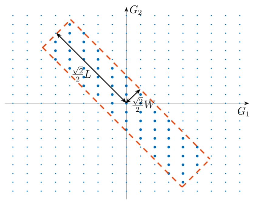
Figure 4.1: Schematic plot of the domain $\mathcal{D}_{W,L}$ in the reciprocal space.

With the discrete Hamiltonian (4.1) and the cutoff (4.2), the DoS of the system is approximated by

$$\underline{{\widehat{\rm Tr}}}_{W,L}\Big{(}g\big{(}\hat{H}^{\mathcal{D}_{W,L}}\big{)}\Big{)}:=\frac{|\Gamma_{1}^{*}||\Gamma_{2}^{*}|}{S_{d,L}}{\rm Tr}\Big{(}g\big{(}\hat{H}^{\mathcal{D}_{W,L}}\big{)}\Big{)},$$ (4.3)

where $S_{d,L}:=\pi^{d/2}L^{d}/2^{d}\varGamma(\frac{d}{2}+1)$ denotes the volume of $d$ dimensional ball with diameter $L$ and $\varGamma$ is the Euler’s gamma function. Here, the pre-factor $|\Gamma_{1}^{*}||\Gamma_{2}^{*}|/S_{d,L}$ is used such that the DoS can be correctly “averaged” to unit volume.

In practical calculations, the trace ${\rm Tr}\big{(}g(\hat{H}^{\mathcal{D}_{W,L}})\big{)}$ on the right-hand side of (4.3) can evaluated once the finite dimensional Hamiltonian $\hat{H}^{\mathcal{D}_{W,L}}$ is obtained. One can either solve the matrix eigenvalue problem to get the eigenvalues $\{\lambda_{i}\}$ of $\hat{H}^{\mathcal{D}_{W,L}}$ and take the sum ${\rm Tr}\big{(}g(\hat{H}^{\mathcal{D}_{W,L}})\big{)}=\sum_{i}g(\lambda_{i})$; or use some kernel polynomial methods (see e.g. [29, 30, 37]) to calculate the diagonal of the matrix $g\big{(}\hat{H}^{\mathcal{D}_{W,L}}\big{)}$ directly.

4.2 Convergence analysis

We will show in this section that the approximate DoS (4.3) converges and provide the convergence rates with respect to $L$ and $W$ respectively. To give a representation of the limit, we need to introduce the “shifted” discrete Hamiltonian.

For $\xi\in\mathbb{R}^{d}$, we define the “shifted” discrete Hamiltonian $\hat{H}(\xi)$ with domain $\mathcal{D}\big{(}\hat{H}(\xi)\big{)}\subset\ell^{2}(\mathcal{R}_{1}^{*}\times\mathcal{R}_{2}^{*})$ by

$$\big{(}\hat{H}(\xi)\big{)}_{{\bf G},{\bf G}^{\prime}}=\frac{1}{2}\big{|}\xi+G_{1}+G_{2}\big{|}^{2}\delta_{G_{1}G_{1}^{{}^{\prime}}}\delta_{G_{2}G_{2}^{{}^{\prime}}}+\hat{V}_{1,G_{1}-G_{1}^{{}^{\prime}}}\delta_{G_{2}G_{2}^{{}^{\prime}}}+\hat{V}_{2,G_{2}-G_{2}^{{}^{\prime}}}\delta_{G_{1}G_{1}^{{}^{\prime}}}$$ (4.4)

for ${\bf G}=(G_{1},G_{2}),~{}{\bf G}^{\prime}=(G_{1}^{{}^{\prime}},G_{2}^{{}^{\prime}})\in\mathcal{R}_{1}^{*}\times\mathcal{R}_{2}^{*}$. The next lemma indicates that the thermodynamic limit of the “local” DoS is well defined in the reciprocal space, whose proof is given in Appendix B.3.

Lemma 4.1.

Let $g\in\Lambda_{\zeta,\delta}$ and $\Omega_{R}({\bf G}):=B_{R}({\bf G})\cap(\mathcal{R}_{1}^{*}\times\mathcal{R}_{2}^{*})$, then the limit $\displaystyle g\big{(}\hat{H}(\xi)\big{)}_{{\bf G},{\bf G}}:=\lim_{R\rightarrow\infty}g\big{(}\hat{H}(\xi)^{\Omega_{R}({\bf G})}\big{)}_{{\bf G},{\bf G}}$ exists.

The following theorem justifies the convergence of the planewave approximations, whose proof is given in Appendix B.4.

Theorem 4.1.

Let $g\in\Lambda_{\zeta,\delta}$, then the limit

$$\underline{{\widehat{\rm Tr}}}\Big{(}g\big{(}\hat{H}\big{)}\Big{)}:=\lim_{W\to\infty}\lim_{L\to\infty}\underline{{\widehat{\rm Tr}}}_{W,L}\Big{(}g\big{(}\hat{H}^{\mathcal{D}_{W,L}}\big{)}\Big{)}$$ (4.5)

exists and

$$\underline{{\widehat{\rm Tr}}}\Big{(}g\big{(}\hat{H}\big{)}\Big{)}=\int_{\mathbb{R}^{d}}g\big{(}\hat{H}(\xi)\big{)}_{{\bf 0},{\bf 0}}~{}{\rm d}\xi.$$ (4.6)

Moreover, there exist positive constants $C$ and $c$ independent of $L$, $W$ and $g$, such that

$$\left|\underline{{\widehat{\rm Tr}}}\Big{(}g\big{(}\hat{H}\big{)}\Big{)}-\underline{{\widehat{\rm Tr}}}_{W,L}\Big{(}g\big{(}\hat{H}^{\mathcal{D}_{W,L}}\big{)}\Big{)}\right|\leq C\delta^{-2}\big{(}L^{-1}+e^{-c\zeta W}\big{)}.$$ (4.7)

Theorem 4.1 provides us explicit convergence rates of the planewave approximation (4.3) of DoS for the incommensurate systems. We see that the approximate errors decay exponentially fast with respect to $W$ but only decay like $\mathcal{O}(L^{-1})$ with respect to $L$. Therefore, to balance the numerical errors and achieve optimal computational cost, one may need a much larger $L$ than $W$ for the planewave cutoffs, see also the shape of $\mathcal{D}_{W,L}$ in Figure 4.1.

Intuitively, the $|G_{1}+G_{2}|$ (truncated by $W$) corresponds to raising the planewave frequencies, and hence achieve fast convergence for smooth problems; while the $|G_{1}-G_{2}|$ (truncated by $L$) corresponds to traversing the reciprocal space, and the convergence of which is determined by the ergodicity (see the first order convergence rate in Lemma B.1). These intuitions can be reflected by the proof of this theorem.

We also need to show that by calculating the planewave approximation (4.3), we are approximating the DoS justified in Section 3. The following theorem proves that the limit of the planewave approximation (4.6) does match the DoS in the real-space formulation (3.5). The proof is given in Appendix B.5.

Theorem 4.2.

Let $g\in\Lambda_{\zeta,\delta}$, then $\displaystyle\underline{\rm Tr}\Big{(}g\big{(}H\big{)}\Big{)}=\underline{{\widehat{\rm Tr}}}\Big{(}g\big{(}\hat{H}\big{)}\Big{)}$.

Since the approximation (4.3) has a slow convergence rate with respect to the cutoff $L$, we will propose an improved scheme based on a uniform sampling of the reciprocal space. Let $K\in\mathbb{N}^{+}$ and $h=W/K$. We first construct a uniform mesh $\mathcal{K}_{h}$ on $[-W,W]^{d}$ with

$$\mathcal{K}_{h}^{W}=\Big{\{}\big{(}x_{k_{1}},\cdots,x_{k_{d}}\big{)},\quad-K\leq k_{i}<K,~{}1\leq i\leq d\Big{\}},\qquad{\rm where}~{}x_{j}=jh.$$ (4.8)

We then approximate the DoS by

$$\underline{\widetilde{\rm Tr}}_{W,L}^{h}\Big{(}g\big{(}\hat{H}^{\mathcal{D}_{W,L}}\big{)}\Big{)}:=h^{d}\sum_{\xi\in\mathcal{K}_{h}^{W}}g\big{(}\hat{H}(\xi)^{\mathcal{D}_{W,L}}\big{)}_{{\bf 0},{\bf 0}}.$$ (4.9)

In practical calculations, one can evaluate $g\big{(}\hat{H}(\xi)^{\mathcal{D}_{W,L}}\big{)}_{{\bf 0},{\bf 0}}$ on the right-hand side of (4.9) directly by using the formla $\sum_{j}g(\lambda_{j}^{\xi})(\psi_{j}^{\xi})_{{\bf 0}}^{2}$, where $(\lambda_{j}^{\xi},\psi_{j}^{\xi})$ are eigenpairs of the matrix $\hat{H}(\xi)^{\mathcal{D}_{W,L}}$. Alternatively, one can approximate the matrix elements of $g\big{(}\hat{H}(\xi)^{\mathcal{D}_{W,L}}\big{)}$ directly by the kernel polynomial methods [30, 31, 37].

The following theorem gives the convergence of the approximation (4.9), which shows that the numerical errors decay exponentially fast with respect to the planewave cutoff and the sampling size. The proof of this theorem is given in Appendix B.6.

Theorem 4.3.

Let $g\in\Lambda_{\zeta,\delta}$, then there exist positive constants $C$ and $c$ that do not depend on $L$, $W$, $h$ and $g$, such that

$$\left|\underline{\widetilde{\rm Tr}}_{W,L}^{h}\Big{(}g\big{(}\hat{H}^{\mathcal{D}_{W,L}}\big{)}\Big{)}-\underline{{\widehat{\rm Tr}}}\Big{(}g\big{(}\hat{H}\big{)}\Big{)}\right|\leq C\big{(}\delta^{-2}e^{-c\delta L}+\delta^{-2}e^{-c\zeta W}+e^{-c\delta/h}\big{)}.$$ (4.10)

Remark 4.1.

We mention that the exponential decay with respect to the quadrature mesh size $h$ comes from the Trapezoidal rule for analytic functions (see the proof in Appendix B.6 or [34]). This result requires the integrand to be over the whole space $\mathbb{R}^{d}$, and can be clearly observed when the cutoff $W$ is sufficiently large (see numerical results, Figure 5.6 and Figure 5.12). However, when the cutoff $W$ is fixed at a small value, one will observe an $\mathcal{O}(h^{2})$ convergence with respect to the mesh size since the integral is on a bounded domain and the tails outside $[-W,W]^{d}$ can not be neglected (see numerical results, Figure 5.6 and Figure 5.12 ). In practice, we will need to balance the errors from truncation $W$ and quadrature mesh size $h$.

5 Numerical experiments

In this section, we will present some numerical experiments for approximating the DoS for some 1D and 2D incommensurate systems. We also ignore the $(d+1)$-th direction in the numerical simulations and perform tests on toy models. All simulations are implemented in open-source Julia packages incommensurate_Pw.jl [36], and performed on a PC with Intel Core i7-CPU (2.2 GHz) with 32GB RAM.

We consider the convergence of numerical approximations of the DoS with some given $g\in\Lambda_{\zeta,\delta}$, and test the decay of (absolute) numerical errors with respect to different parameters. The results obtained by using sufficiently large discretization are taken to be the reference (exact solution).

Example 1. (1D incommensurate system) Considering the following Hamiltonian

$$H=-\frac{1}{2}\Delta+v_{1}+v_{2}$$ (5.1)

with

$$v_{1}(x)=\sum_{G_{1}\in\mathcal{R}^{*}_{1}}e^{-\gamma|G_{1}|^{2}}e^{iG_{1}\cdot x}\qquad{\rm and}\qquad v_{2}(x)=\sum_{G_{2}\in\mathcal{R}^{*}_{2}}e^{-\gamma|G_{2}|^{2}}e^{iG_{2}\cdot x}.$$ (5.2)

We take the reciprocal lattices $\mathcal{R}^{*}_{1}=2\pi/L_{1}\mathbb{Z}$ and $\mathcal{R}^{*}_{2}=2\pi/L_{2}\mathbb{Z}$ with $L_{1}=\sqrt{5}-1$ and $L_{2}=2$. To compute the DoS that corresponds to the total energy under a Fermi-Dirac distribution, we take $g$ as

$$g_{\beta,\mu}(x)=\frac{x}{1+e^{\beta(x-\mu)}},$$ (5.3)

where $\mu$ is a fixed chemical potential and $\beta:=(k_{B}T)^{-1}$ is the inverse temperature $T$ with $k_{B}$ the Boltzmann constant. Note that the operator $H$ is bounded from below, we are not concerned with the behavior of $g_{\beta,\mu}$ as $x\to-\infty$. We see that $g\in\Lambda_{\zeta,\delta}$ with both parameters $\delta$ and $\zeta$ depending on $\beta$. In the low-temperature regime (corresponding to large $\beta$), $g$ will vanish quickly as $x$ increases, so the convergence of numerical approximations for the DoS will mainly be affected by how far the singularity of $g$ is away from the real axis, i.e. the parameter $\delta$. In the high-temperature regime (corresponding to small $\beta$), $g$ will be sufficiently smooth, so the decay of $g$ will play a more important role for the convergence of numerical approximations.

We first test the convergence of the planewave approximations by the numerical scheme (4.3). We observe from Figure 5.6 that the numerical errors decay at a first order with respect to $L$, and from Figure 5.6 that the errors decay exponentially fast with respect to $W$. The results match perfectly with our theoretical prediction in Theorem 4.1. We also compare the convergence rates for potentials with different regularity (indicated by $\gamma$ in (2.3)), and see that the planewave approximations can converge significantly faster with respect to $W$ with more regular potentials.

We then perform the simulations by the numerical scheme (4.9). We show the decay of numerical errors with respect to $L$ in Figure 5.6, from which we observe exponential convergence rates and that smaller $\beta$’s lead to faster decay rates. We further present the numerical errors with respect to $W$ in Figure 5.6, from which we see that the errors decay exponentially fast and that bigger $\zeta$’s give faster convergence rates. These numerical results fit our theory very well.

Finally, we test the convergence with respect to the quadrature mesh size $h$. We show the numerical errors in Figure 5.6 and Figure 5.6 for different $W$ respectively. We observe an exponentially fast decay with respect to $h$ when $W$ is large, and a second order decay with respect to $h$ when $W$ is small (where the reference is taken by using the same $W$ and a very small $h$). These observations match perfectly with our theoretical predictions in Theorem 4.3 and Remark 4.1.

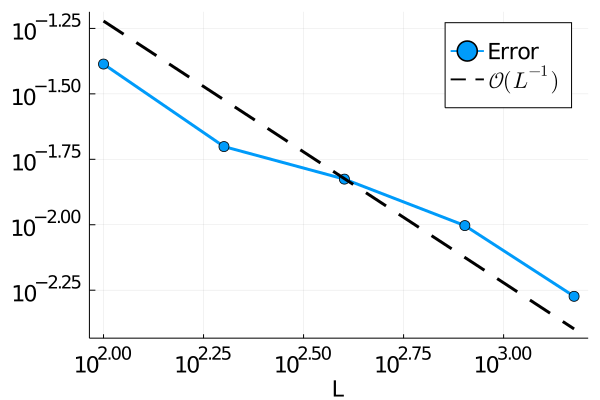
Figure 5.1: (Example 1) Error decay with respect to $L$ by scheme (4.3).

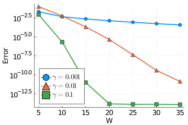
Figure 5.2: (Example 1) Error decay with respect to $W$ by scheme (4.3).

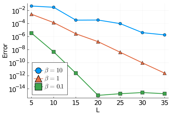
Figure 5.3: (Example 1) Error decay with respect to $L$ by scheme (4.9).

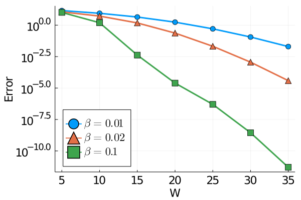
Figure 5.4: (Example 1) Error decay with respect to $W$ by scheme (4.9).

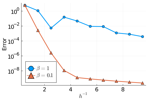
Figure 5.5: (Example 1) Error decay with respect to $h$ by scheme (4.9) with $W=25$.

Figure 5.6: (Example 1) Error decay with respect to $h$ by scheme (4.9) with $W=5$.

Example 2. (2D incommensurate system) Consider a two-dimensional incommensurate system obtained by stacking two periodic lattices together, in which one layer is rotated by an angle $\theta=\pi/10$ with respect to the other. More precisely, we take $\mathcal{R}_{1}=A_{1}\mathbb{Z}^{2}$ and $\mathcal{R}_{2}=A_{2}\mathbb{Z}^{2}$ with

$$A_{1}=2\left[\begin{gathered}\begin{matrix}1&0\\ 0&1\end{matrix}\end{gathered}\right],\qquad\qquad A_{2}=2\left[\begin{gathered}\begin{matrix}\cos(\theta)&\cos(\theta+\frac{\pi}{2})\\ \sin(\theta)&\sin(\theta+\frac{\pi}{2})\end{matrix}\end{gathered}\right].$$

The potentials are given in the same form of (5.2) and the DoS is the same as that in (5.3).

For the numerical scheme (4.3), the numerical errors with respect to $L$ and $W$ are presented in Figure 5.12 and Figure 5.12 respectively, which are consistent with our theory. For the numerical scheme (4.9), we show the convergence of the numerical errors with respect to $L$ and $W$ with different $\beta$ in Figure 5.12 and Figure 5.12 respectively. Moreover, we present the convergence with respect to mesh size $h$ in Figure 5.12 and Figure 5.12, for large and small cutoffs of $W$ respectively. All these results match perfectly with our theoretical perspective.

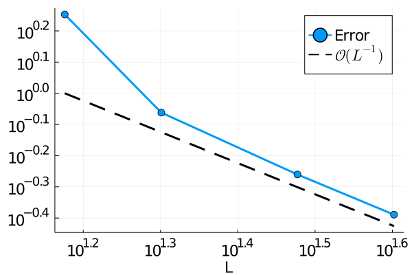
Figure 5.7: (Example 2) Error decay with respect to $L$ by scheme (4.3).

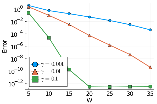
Figure 5.8: (Example 2) Error decay with respect to $W$ by scheme (4.3).

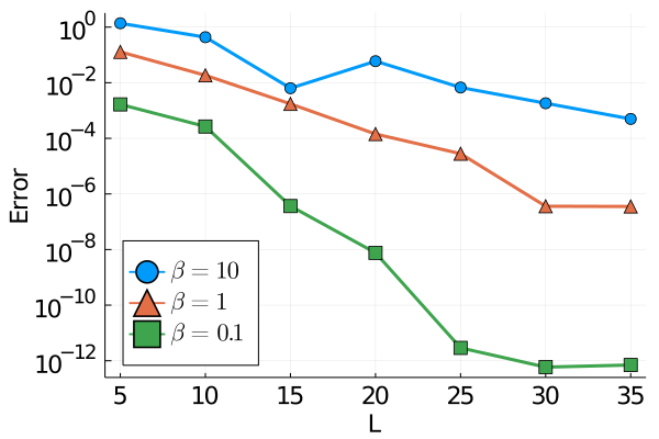
Figure 5.9: (Example 2) Error decay with respect to $L$ by scheme (4.9).

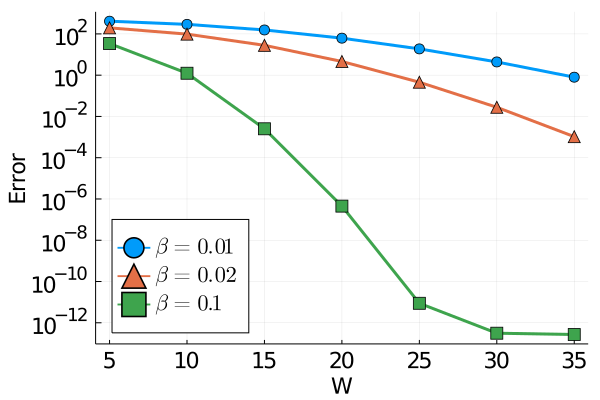
Figure 5.10: (Example 2) Error decay with respect to $W$ by scheme (4.9).

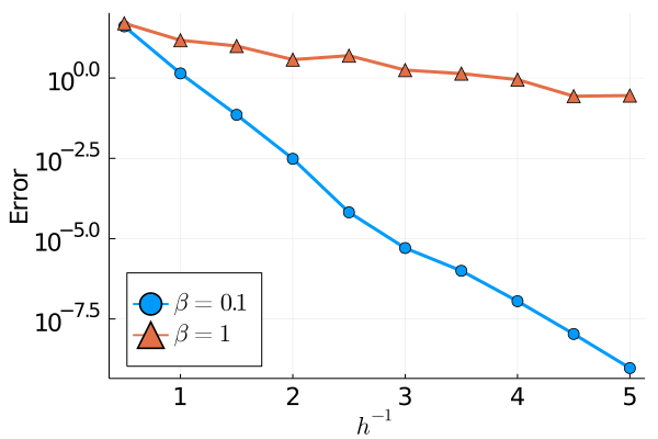
Figure 5.11: (Example 2) Error decay with respect to $h$ by scheme (4.9) with $W=30$

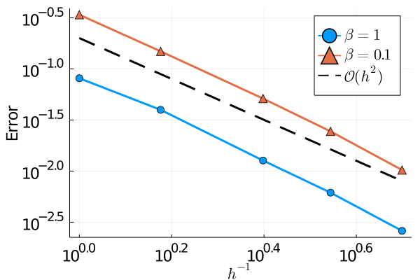
Figure 5.12: (Example 2) Error decay with respect to $h$ by scheme (4.9) with $W=5$

6 Conclusions

In this paper, we provide a generic framework to study the continuous electronic structure models for incommensurate systems. We show that most physical observables of the system is well defined and can be approximated efficiently by some planewave approximations. In our future work, we will generalize the theory and numerical algorithms to other observables such as conductivity, optical response, and topological Chern number. We will also extend to more complex nonlinear models such as density functional theory.

Appendix A The symbolic calculus of pseudodifferential operators

The symbolic calculus is developed since pseudodifferential operators form an algebra, which allows one to transform operations in terms of these differential operators to the associated symbols [12, 17, 33, 41]. In particular, it provides an avenue for describing the composition of several operators using functional calculus of pseudodifferential operators by working on the operators’ symbol functions. In the context of our work, the DoS is formulated as an integral of the symbol functions and the analysis can be performed conveniently by symbolic calculus. In this appendix, we will briefly review some symbolic calculus of pseudodifferential operators which will be heavily used in our analysis.

Let $a:\mathbb{R}^{d}\times\mathbb{R}^{d}\rightarrow\mathbb{R}$ be given by $a(x,\xi)=\sum_{\alpha}p_{\alpha}(x)\xi^{\alpha}$. Denote by $\alpha=(\alpha_{1},\cdots,\alpha_{d})$, $D^{\alpha}=(-i\partial_{1})^{\alpha_{1}}\cdots(-i\partial_{d})^{\alpha_{d}}$ with $i=\sqrt{-1}$. Define a differential operator

$$a(x,D):=\sum_{\alpha}p_{\alpha}(x)D^{\alpha},$$

such that for any $u(x)\in\mathscr{S}(\mathbb{R}^{d})$,

$$a(x,D)u(x)=\frac{1}{(2\pi)^{d}}\int_{\mathbb{R}^{d}}a(x,\xi)e^{ix\cdot\xi}\hat{u}(\xi){~{}{\rm d}}\xi=\frac{1}{(2\pi)^{d}}\int_{\mathbb{R}^{d}}\int_{\mathbb{R}^{d}}a(x,\xi)e^{i(x-y)\cdot\xi}u(y){~{}{\rm d}}y{~{}{\rm d}}\xi.$$ (A.1)

Then we call the function $a(x,\xi)$ as the symbol of the operator $a(x,D)$. Taking $a(x,\xi)$ belongs to one of a number of different classes of symbols, then the Fourier integral representation (A.1) defines pseudodifferential operators (from $\mathscr{S}(\mathbb{R}^{d})$ to $\mathscr{S}(\mathbb{R}^{d})$) [33, 41]. The algebraic behavior of symbols dictates the properties of their associated pseudodifferential operators. For example, for a class of symbols in $S({\bf 1})$ (defined in (3.2)), the associated operator is continuous from $L^{2}(\mathbb{R}^{d})$ into $L^{2}(\mathbb{R}^{d})$ (see [41, Theorem 4.23]). Another example is that for decaying order function $\big{(}\mathfrak{m}(x,\xi)\to 0,\ {\rm as}\ (x,\xi)\to\infty\big{)}$ (see (3) for the definition of order function), the related pseudodifferential operator is a compact operator (see [41, Theorem 4.28]). Note that $a\#b$ represents the composed symbol of $a$ and $b$ in Appendices.

The following lemmas for symbolic calculus are crucial for our analysis. Lemma A.1 shows that the composition of two pseudodifferential operators gives a pseudodifferential operator. Lemma A.2 specifies the symbol class of functional calculus of a pseudodifferential operator. Lemma A.3 gives a sufficient condition for a pesudodifferential operator to be of trace class and provides a formula evaluating the trace in terms of the symbols. The proofs of these lemmas are referred to the related textbooks.

Lemma A.1.

[12, Theorem 7.9] If $a\in S(\mathfrak{m}_{1})$ and $b\in S(\mathfrak{m}_{2})$, then the symbol of the composition operator

$$(a\#b)(x,D):=a(x,D)b(x,D)$$

satisfies $a\#b\in S(\mathfrak{m}_{1}\mathfrak{m}_{2})$.

Lemma A.2.

[1, Theorem 4] Let $H$ be a pseudodifferential operator with the real-valued symbol $\sigma[H]\in S(\mathfrak{m})$ satisfying $\mathfrak{m}\geq 1$. Let $g\in C^{\infty}(\mathbb{R})$ be a “symbol of order $p$”, i.e. such that

$$\left|\frac{d^{k}g(t)}{dt^{k}}\right|\leq C_{k}\big{(}1+|t|\big{)}^{p-k}\quad{\rm for}~{}p\in\mathbb{R},~{}k\in\mathbb{N}.$$

Then we have

$$\sigma[g(H)]\in S(\mathfrak{m}^{p}).$$

Lemma A.3.

[12, Thorem 9.4] Let $a\in\mathscr{S}^{\prime}(\mathbb{R}^{d}\times\mathbb{R}^{d})$ satisfy

$$\sum_{|\alpha+\beta|\leq 2d+1}\big{\|}\partial^{\alpha}_{x}\partial^{\beta}_{\xi}a\big{\|}_{L^{1}}<\infty.$$ (A.2)

Then the operator $a(x,D)$ is of trace class and

$$\|a(x,D)\|_{\rm tr}\leq C_{d}\sum_{|\alpha+\beta|\leq 2d+1}\|\partial^{\alpha}_{x}\partial^{\beta}_{\xi}a\|_{L^{1}},\quad{\rm Tr}(a(x,D))=\frac{1}{(2\pi)^{d}}\int_{\mathbb{R}^{d}}\int_{\mathbb{R}^{d}}a(x,\xi)~{}{\rm d}\xi~{}{\rm d}x.$$

Appendix B Proofs

B.1 Proof of Lemma 3.1

Proof.

We have from the definition of $\chi_{j}$ that for any $s>0$ and $\beta\in\mathbb{N}^{d}$,

$$\sup_{x\in\mathbb{R}^{d}}\big{(}1+|x-j|^{2}\big{)}^{s}\left|\partial^{\beta}\chi_{j}(x)\right|<\infty\qquad\forall~{}j\in\mathbb{Z}^{d}.$$

This estimate together with the symbolic calculus and the definition (3.2) implies

$$\sigma[\chi_{j}]=\chi_{j}(x)\in S\Big{(}\big{(}1+|x-j|^{2}\big{)}^{-s}\Big{)}\qquad\forall~{}j\in\mathbb{Z}^{d},\ s>0.$$

By using Lemma A.1 and Lemma A.2, we see that the symbol of the operator $\chi_{j}g(H)\chi_{k}$ satisfies

$$\Big{(}\sigma[\chi_{j}]\#\sigma[g(H)]\#\sigma[\chi_{k}]\Big{)}\in S\Big{(}\big{(}1+|x-j|^{2}\big{)}^{-s}\big{(}1+|\xi|^{2}\big{)}^{-s}\big{(}1+|x-k|^{2}\big{)}^{-s}\Big{)}$$ (B.1)

for any $j,k\in\mathbb{Z}^{d}\cap B_{R}$ and $s>0$. For $s>2d$, we see that the order function on the right-hand side of (B.1) belongs to $L^{1}(\mathbb{R}^{d}\times\mathbb{R}^{d})$ since

$$\int_{\mathbb{R}^{d}}\int_{\mathbb{R}^{d}}\big{(}1+|x-j|^{2}\big{)}^{-s}\big{(}1+|\xi|^{2}\big{)}^{-s}\big{(}1+|x-k|^{2}\big{)}^{-s}{~{}{\rm d}}\xi{~{}{\rm d}}x\\[4.30554pt] \leq\int_{\mathbb{R}^{d}}\big{(}1+|\xi|^{2}\big{)}^{-s}{~{}{\rm d}}\xi\int_{\mathbb{R}^{d}}\big{(}1+|x-j|^{2}\big{)}^{-s}\big{(}1+|x-k|^{2}\big{)}^{-s}{~{}{\rm d}}x\leq C{\big{(}1+|j-k|^{2}\big{)}^{-s}},$$

where $C>0$ is a constant depending only on $d$. Then we have from (3.2) and Lemma A.3 that $\chi_{j}g(H)\chi_{k}$ is of trace class and

$${\rm Tr}\big{(}\chi_{j}g(H)\chi_{k}\big{)}\leq C{\big{(}1+\left|j-k\right|^{2}\big{)}^{-s}},$$

where $C>0$ is a constant depending on $d$. This completes the proof of Lemma 3.1. ∎

B.2 Proof of Theorem 3.1

To prove Theorem 3.1, we will need the following lemma (see [3, Proposition 2.4] and [30, Theorem 2.1 and Page 14]), which mirrors the ergodicity of incommensurate system. This is a key feature and also plays an important role in the theory and algorithms for planewave approximations. We refer to [30, Page 13-14] for the proof.

Lemma B.1.

Let $\mathcal{R}_{1}$ and $\mathcal{R}_{2}$ be incommensurate, with $\Gamma_{1}$ and $\Gamma_{2}$ the associated unit cells respectively. Let $k\in\{1,2\}$, if $f\in C(\mathbb{R}^{d})$ is periodic with respect to $\mathcal{R}_{k}$, then

$$\lim_{R\to\infty}\frac{1}{\#\mathcal{R}_{\bar{k}}\cap B_{R}}\sum_{\ell\in\mathcal{R}_{\bar{k}}\cap B_{R}}f(\ell)=\frac{1}{|\Gamma_{k}|}\int_{\Gamma_{k}}f(b)~{}{\rm d}b,$$

where $\bar{k}=1$ if $k=2$ and $\bar{k}=2$ if $k=1$. Moreover, there exists a constant $C>0$ independent of $R$, such that

$$\left|\frac{1}{\#\mathcal{R}_{j}\cap B_{R}}\sum_{\ell\in\mathcal{R}_{j}\cap B_{R}}f(\ell)-\frac{1}{|\Gamma_{k}|}\int_{\Gamma_{k}}f(b)~{}{\rm d}b\right|\leq CR^{-1}.$$ (B.2)

Proof of Theorem 3.1..

We first define the following region that is slightly adjusted from $B_{R}$:

$$\tilde{B}_{R}:=\cup_{j\in\mathcal{R}_{1}\cap B_{R}}\big{(}j+\Gamma_{1}\big{)}.$$

For $b_{1},b_{2}\in\mathbb{R}^{d}$, the symbol of the operators $H(b_{1},b_{2})$ (defined in (3.4)) are given by

$$\sigma[H(b_{1},b_{2})](x,\xi)=\frac{1}{2}|\xi|^{2}+v_{1}(x+b_{1})+v_{2}(x+b_{2}),\qquad(x,\xi)\in\mathbb{R}^{d}\times\mathbb{R}^{d}.$$

For $g\in\mathscr{S}(\mathbb{R})$, we observe that the function of a pseudodifferential operator can be estimated from their resolvent by using the Helffer-Sjöstrand formula [41, Theorem 14.8 and Page 358], then we have

$$\sigma[g(H)](x,\xi)=\sigma[g(H(x,x))](0,\xi).$$ (B.3)

Note that Lemma 3.1 implies that $\chi_{j}g(H)\chi_{k}$ is of trace class for any $j,k\in\mathbb{Z}^{d}$, which together with Lemma A.3 and the property of $\chi_{j}$ leads to

$$\hskip-5.69046pt\underline{\rm Tr}_{R}(g(H))=\frac{1}{|B_{R}|}\sum_{j,k\in\mathbb{Z}^{d}\cap B_{R}}{\rm Tr}\big{(}\chi_{j}g(H)\chi_{k}\big{)}$$

$$=\frac{1}{(2\pi)^{d}}\frac{1}{|B_{R}|}\int_{\mathbb{R}^{d}}\int_{\mathbb{R}^{d}}\sum_{j,k\in\mathbb{Z}^{d}\cap B_{R}}\Big{(}\sigma[\chi_{j}]\#\sigma[g(H)]\#\sigma[\chi_{k}]\Big{)}(x,\xi){~{}{\rm d}}\xi{~{}{\rm d}}x$$

$$=\frac{1}{(2\pi)^{d}}\frac{1}{|B_{R}|}\int_{\mathbb{R}^{d}\backslash\tilde{B}_{R}}\int_{\mathbb{R}^{d}}\sum_{j,k\in\mathbb{Z}^{d}\cap B_{R}}\Big{(}\sigma[\chi_{j}]\#\sigma[g(H)]\#\sigma[\chi_{k}]\Big{)}(x,\xi){~{}{\rm d}}\xi{~{}{\rm d}}x$$

$$\quad+\frac{1}{(2\pi)^{d}}\frac{1}{|B_{R}|}\int_{\tilde{B}_{R}}\int_{\mathbb{R}^{d}}\sum_{j,k\in\mathbb{Z}^{d}\cap B_{R}}\Big{(}\sigma[\chi_{j}]\#\sigma[g(H)]\#\sigma[\chi_{k}]\Big{)}(x,\xi){~{}{\rm d}}\xi{~{}{\rm d}}x$$

Then we can estimate

$$\left|\underline{\rm Tr}_{R}(g(H))-\frac{1}{|\Gamma_{1}||\Gamma_{2}|}\int_{\Gamma_{1}}\int_{\Gamma_{2}}\int_{\mathbb{R}^{d}}\sigma[g(H(b_{1},b_{2}))](0,\xi){~{}{\rm d}}\xi{~{}{\rm d}}b_{2}{~{}{\rm d}}b_{1}\right|$$

$$\leq\frac{1}{(2\pi)^{d}}\Bigg{(}\left|\frac{1}{|B_{R}|}\int_{\mathbb{R}^{d}\backslash\tilde{B}_{R}}\int_{\mathbb{R}^{d}}\sum_{j,k\in\mathbb{Z}^{d}\cap B_{R}}\Big{(}\sigma[\chi_{j}]\#\sigma[g(H)]\#\sigma[\chi_{k}]\Big{)}(x,\xi){~{}{\rm d}}\xi{~{}{\rm d}}x\right|$$

$$+\left|\frac{1}{\big{|}B_{R}\big{|}}\int_{\tilde{B}_{R}}\int_{\mathbb{R}^{d}}\Bigg{(}\sum_{j,k\in\mathbb{Z}^{d}\cap B_{R}}\Big{(}\sigma[\chi_{j}]\#\sigma[g(H)]\#\sigma[\chi_{k}]\Big{)}(x,\xi)-\sigma[g(H)](x,\xi)\Bigg{)}{~{}{\rm d}}\xi{~{}{\rm d}}x\right|$$

$$+\left|\frac{1}{\big{|}B_{R}\big{|}}\int_{\tilde{B}_{R}}\int_{\mathbb{R}^{d}}\sigma[g(H)](x,\xi){~{}{\rm d}}\xi{~{}{\rm d}}x-\frac{1}{|\Gamma_{1}||\Gamma_{2}|}\int_{\Gamma_{1}}\int_{\Gamma_{2}}\int_{\mathbb{R}^{d}}\sigma[g(H(b_{1},b_{2}))](0,\xi){~{}{\rm d}}\xi{~{}{\rm d}}b_{2}{~{}{\rm d}}b_{1}\right|$$

$$=:T_{1}+T_{2}+T_{3}.$$

The first term $T_{1}$ can easily be estimated by $\mathcal{O}(R^{-1})$ by using (B.1).

We then estimate the second term $T_{2}$. Denote by

$$S_{R}(x,\xi):=\sum_{j,k\in\mathbb{Z}^{d}\cap B_{R}}\Big{(}\sigma[\chi_{j}]\#\sigma[g(H)]\#\sigma[\chi_{k}]\Big{)}(x,\xi)\qquad{\rm for}\ x\in\mathbb{R}^{d},\ \xi\in\mathbb{R}^{d}.$$ (B.4)

Let $s>2d$, we have that for $x\in\tilde{B}_{R}$ and $\xi\in\mathbb{R}^{d}$,

$$\big{|}\sigma[g(H)](x,\xi)-S_{R}(x,\xi)\big{|}$$

$$\leq \sum_{j\in\mathbb{Z}^{d}\cap B_{R}^{c}}\sum_{k\in\mathbb{Z}^{d}}\left|\Big{(}\sigma[\chi_{j}]\#\sigma[g(H)]\#\sigma[\chi_{k}]\Big{)}(x,\xi)\right|+\sum_{j\in\mathbb{Z}^{d}}\sum_{k\in\mathbb{Z}^{d}\cap B_{R}^{c}}\left|\Big{(}\sigma[\chi_{j}]\#\sigma[g(H)]\#\sigma[\chi_{k}]\Big{)}(x,\xi)\right|$$

$$\leq C\big{(}1+|\xi|^{2}\big{)}^{-s}\sum_{j\in\mathbb{Z}^{d}\cap B_{R}^{c}}\sum_{k\in\mathbb{Z}^{d}}\big{(}1+|x-j|^{2}\big{)}^{-s}\big{(}1+|x-k|^{2}\big{)}^{-s}$$

$$\leq C\big{(}1+|\xi|^{2}\big{)}^{-s}\Big{(}1+\big{|}R-|x|\big{|}^{2}\Big{)}^{d/2-s},$$

where the constants $C$ do not depend on $R$. Then we have

$$T_{2}\leq \frac{1}{(2\pi)^{d}}\frac{1}{|B_{R}|}\int_{\tilde{B}_{R}}\int_{\mathbb{R}^{d}}\big{|}\sigma[g(H)](x,\xi)-S_{R}(x,\xi)\big{|}{~{}{\rm d}}\xi{~{}{\rm d}}x$$

$$\leq \frac{C}{|B_{R}|}\int_{\mathbb{R}^{d}}\big{(}1+|\xi|^{2}\big{)}^{-s}~{}{\rm d}\xi\int_{\tilde{B}_{R}}\Big{(}1+\big{|}R-|x|\big{|}^{2}\Big{)}^{d/2-s}~{}{\rm d}x\leq\mathcal{O}(R^{-1}).$$

For the third term $T_{3}$, we have that

$$T_{3}\leq\frac{1}{(2\pi)^{d}}\Bigg{(}\bigg{(}1-\frac{|B_{R}|}{|\tilde{B}_{R}|}\bigg{)}\frac{1}{|B_{R}|}\int_{\tilde{B}_{R}}\int_{\mathbb{R}^{d}}\sigma[g(H)](x,\xi){~{}{\rm d}}\xi{~{}{\rm d}}x\\ \quad+\left|\frac{1}{|\tilde{B}_{R}|}\int_{\tilde{B}_{R}}\int_{\mathbb{R}^{d}}\sigma[g(H)](x,\xi){~{}{\rm d}}\xi{~{}{\rm d}}x-\frac{1}{|\Gamma_{1}||\Gamma_{2}|}\int_{\Gamma_{1}}\int_{\Gamma_{2}}\int_{\mathbb{R}^{d}}\sigma[g(H(b_{1},b_{2}))](0,\xi){~{}{\rm d}}\xi{~{}{\rm d}}b_{2}{~{}{\rm d}}b_{1}\right|\Bigg{)}.$$ (B.5)

Moreover, we obtain by using (B.3) that

$$\quad\frac{1}{|\tilde{B}_{R}|}\int_{\tilde{B}_{R}}\int_{\mathbb{R}^{d}}\sigma[g(H)](x,\xi){~{}{\rm d}}\xi{~{}{\rm d}}x$$

$$=\frac{1}{|\tilde{B}_{R}|}\int_{\tilde{B}_{R}}\int_{\mathbb{R}^{d}}\sigma[g(H(x,x))](0,\xi){~{}{\rm d}}\xi{~{}{\rm d}}x$$

$$=\frac{1}{|\Gamma_{1}||\#\mathcal{R}_{1}\cap B_{R}|}\sum_{\ell\in\mathcal{R}_{1}\cap B_{R}}\int_{\Gamma_{1}}\int_{\mathbb{R}^{d}}\sigma[g(H(b_{1}+\ell,b_{1}+\ell))](0,\xi){~{}{\rm d}}\xi{~{}{\rm d}}b_{1}$$

$$=\frac{1}{|\Gamma_{1}||\#\mathcal{R}_{1}\cap B_{R}|}\sum_{\ell\in\mathcal{R}_{1}\cap B_{R}}\int_{\Gamma_{1}}\int_{\mathbb{R}^{d}}\sigma[g(H(b_{1},{\rm mod}_{2}(b_{1}+\ell))](0,\xi){~{}{\rm d}}\xi{~{}{\rm d}}b_{1}.$$

This together with Lemma B.1 and (B.5) implies that $T_{3}$ can be bounded by $\mathcal{O}(R^{-1})$.

By taking into accounts all the above estimates, we see that the $R\rightarrow\infty$ limit of $\underline{\rm Tr}_{R}(g(H))$ exists, which is consistent with the right-hand side of (3.5). This completes the proof. ∎

B.3 Proof of Lemma 4.1

We will show in the following a stronger result than Lemma 4.1, which not only justifies the thermodynamic limit of the “local” DoS, but also provide exponential convergence rates to this limit. Since the first error bound has an undesirable dependence on $\delta$ in the exponent, we provide an improved truncation with a significantly better error bound in the $G_{1}+G_{2}$ direction.

Lemma B.2.

Let $\xi\in\mathbb{R}^{d}$, $g\in\Lambda_{\zeta,\delta}$, ${\bf G}=(G_{1},G_{2})\in\mathcal{R}_{1}^{*}\times\mathcal{R}_{2}^{*}$ and $\Omega_{R}({\bf G}):=B_{R}({\bf G})\cap(\mathcal{R}_{1}^{*}\times\mathcal{R}_{2}^{*})$.

• Then the limit

  $$g\big{(}\hat{H}(\xi)\big{)}_{{\bf G},{\bf G}}:=\lim_{R\to\infty}g\big{(}\hat{H}(\xi)^{\Omega_{R}({\bf G})}\big{)}_{{\bf G},{\bf G}}$$ (B.6)

  exists. Furthermore, there exist positive constants $C$ and $c$ independent of $R$, such that

  $$\left|g\big{(}\hat{H}(\xi)^{\Omega_{R}({\bf G})}\big{)}_{{\bf G},{\bf G}}-g\big{(}\hat{H}(\xi)\big{)}_{{\bf G},{\bf G}}\right|\leq C\delta^{-2}e^{-c\delta R}.$$ (B.7)

• If $\Omega_{R}({\bf G})$ is replaced by

  $$\mathcal{D}_{W,L}({\bf G}):=\Big{\{}\big{(}G_{1}^{{}^{\prime}},G_{2}^{{}^{\prime}}\big{)}\in\mathcal{R}_{1}^{*}\times\mathcal{R}_{2}^{*}:~{} \big{|}(G_{1}^{{}^{\prime}}-G_{1})+(G_{2}^{{}^{\prime}}-G_{2})\big{|}\leq W,$$

  $$\big{|}(G_{1}^{{}^{\prime}}-G_{1})-(G_{2}^{{}^{\prime}}-G_{2})\big{|}\leq L\Big{\}},$$

  then there exist positive constants $C$ and $c$ independent of $W$ and $L$, such that

  $$\left|g\big{(}\hat{H}(\xi)^{\mathcal{D}_{W,L}({\bf G})}\big{)}_{{\bf G},{\bf G}}-g\big{(}\hat{H}(\xi)\big{)}_{{\bf G},{\bf G}}\right|\leq C\delta^{-2}\big{(}e^{-c\delta L}+e^{-c\zeta W}\big{)}.$$ (B.8)

Proof.

(i) Let $\Omega\subset\mathcal{R}_{1}^{*}\times\mathcal{R}_{2}^{*}$ such that $\Omega\supsetneq\Omega_{R}({\bf G})$. Let $\hat{H}(\xi)^{\Omega}\in\mathbb{R}^{\#\Omega\times\#\Omega}$ be the matrix whose elements are given by (4.1).

We first expand the matrix $\hat{H}^{\Omega_{R}({\bf G})}$ to a “bigger” matrix $\hat{H}(\xi)_{\Omega}^{\Omega_{R}({\bf G})}\in\mathbb{C}^{\#\Omega\times\#\Omega}$ by filling zero matrix elements, i.e.

$$\big{(}\hat{H}(\xi)_{\Omega}^{\Omega_{R}({\bf G})}\big{)}_{{\bf G}^{\prime},{\bf G}^{\prime\prime}}=\left\{\begin{array}[]{ll}\big{(}\hat{H}(\xi)^{\Omega_{R}({\bf G})}\big{)}_{{\bf G}^{\prime},{\bf G}^{\prime\prime}}&{\rm if\ {\bf G}^{\prime},{\bf G}^{\prime\prime}\in\Omega_{R}({\bf G})},\\[4.30554pt] \quad 0&{\rm otherwise}.\end{array}\right.$$ (B.11)

Using the decay of $|\hat{V}_{j,G}|$ in (2.3), we have

$$\left|\big{(}\hat{H}(\xi)_{\Omega}^{\Omega_{R}({\bf G})}\big{)}_{{\bf G}^{\prime},{\bf G}^{\prime\prime}}\right|\leq Ce^{-\gamma|{\bf G}^{\prime}-{\bf G}^{\prime\prime}|}\qquad{\rm for}~{}{\bf G}^{\prime},{\bf G}^{\prime\prime}\in\Omega.$$ (B.12)

For $g\in\Lambda_{\zeta,\delta}$, we can find a contour $\mathscr{C}_{R}\subset\mathbb{C}$ such that it encloses all the eigenvalues of $\hat{H}^{\Omega}(\xi)$ and $\hat{H}(\xi)_{\Omega}^{\Omega_{R}({\bf G})}$, and satisfies

$$\min\Bigg{\{}{\rm dist}\big{(}z,\mathfrak{s}(g)\big{)},~{}{\rm dist}\left(z,\mathfrak{d}\big{(}\hat{H}(\xi)^{\Omega_{R}({\bf G})}\big{)}\right),~{}{\rm dist}\big{(}z,\{0\}\big{)}\Bigg{\}}\geq\frac{\delta}{2}\qquad{\rm and}$$

$$\max\Bigg{\{}{\rm dist}\big{(}z,\mathfrak{s}(g)\big{)},~{}{\rm dist}\left(z,\mathfrak{d}\big{(}\hat{H}(\xi)^{\Omega_{R}({\bf G})}\big{)}\right),~{}{\rm dist}\big{(}z,\{0\}\big{)}\Bigg{\}}\leq\delta$$ (B.13)

for any $z\in\mathscr{C}_{R}$, where $\mathfrak{s}(g)$ represents the non-analytic region of $g$ and $\mathfrak{d}(\cdot)$ represents the spectrum set. By using a Combes–Thomas type estimate [9] (see similar arguments in [8, Lemma 6]), we have from (B.12) and (B.3) that

$$\left|\Big{(}\big{(}z-\hat{H}(\xi)^{\Omega}\big{)}^{-1}\Big{)}_{{\bf G}^{\prime},{\bf G}^{\prime\prime}}\right|\leq\frac{1}{\delta}e^{-\bar{\gamma}\delta|{\bf G}^{\prime}-{\bf G}^{\prime\prime}|},\quad\left|\Big{(}\big{(}z-\hat{H}(\xi)_{\Omega}^{\Omega_{R}({\bf G})}\big{)}^{-1}\Big{)}_{{\bf G}^{\prime},{\bf G}^{\prime\prime}}\right|\leq\frac{1}{\delta}e^{-\bar{\gamma}\delta|{\bf G}^{\prime}-{\bf G}^{\prime\prime}|}$$

with some constant $\bar{\gamma}>0$ depending on $\gamma$. We can derive from the above decay estimates of resolvents and a direct calculation that

$$\left|\Big{(}\big{(}z-\hat{H}(\xi)^{\Omega}\big{)}^{-1}\Big{)}_{{\bf G},{\bf G}}-\Big{(}\big{(}z-\hat{H}(\xi)^{\Omega_{R}({\bf G})}\big{)}^{-1}\Big{)}_{{\bf G},{\bf G}}\right|\leq C\delta^{-2}e^{-c\delta R},$$ (B.14)

where $c>0$ is a constant depending on $\gamma$.

For $g\in\Lambda_{\zeta,\delta}$, we can exploit the contour integral representation and get

$$\quad\left|g\big{(}\hat{H}(\xi)^{\Omega}\big{)}_{{\bf G},{\bf G}}-g\big{(}\hat{H}(\xi)^{\Omega_{R}({\bf G})}\big{)}_{{\bf G},{\bf G}}\right|$$

$$=\left|\frac{1}{2\pi i}\oint_{\mathscr{C}_{R}}g(z)\Bigg{(}\Big{(}\big{(}z-\hat{H}^{\Omega}(\xi)\big{)}^{-1}\Big{)}_{{\bf G},{\bf G}}-\Big{(}\big{(}z-\hat{H}(\xi)_{\Omega}^{\Omega_{R}({\bf G})}\big{)}^{-1}\Big{)}_{{\bf G},{\bf G}}\Big{)}~{}{\rm d}z\right|$$

$$\leq C\delta^{-2}e^{-c\delta R}\frac{1}{2\pi}\oint_{\mathscr{C}_{R}}\big{|}g(z)\big{|}~{}{\rm d}z,$$ (B.15)

where the estimate (B.14) is used for the last inequality. Note that the exponential decay condition in the definition (2.4) of $\Lambda_{\zeta,\delta}$ implies that $\oint_{\mathscr{C}_{R}}\big{|}g(z)\big{|}~{}{\rm d}z$ is uniformly bounded by some constant as $R\rightarrow\infty$. This together with (B.3) indicates that $g\big{(}\hat{H}(\xi)^{\Omega_{R}({\bf G})}\big{)}_{{\bf G},{\bf G}}$ converge to some limit uniformly. Then the convergence rate (B.7) is a direct consequence of (B.3).

(ii) By using the result and arguments in the proof for (i), it is only necessary for us to justify the convergence rate with respect to $W$, that is,

$$\left|g\big{(}\hat{H}(\xi)^{\mathcal{D}_{W^{\prime},L}({\bf G})}\big{)}_{{\bf G},{\bf G}}-g\big{(}\hat{H}(\xi)^{\mathcal{D}_{W,L}({\bf G})}\big{)}_{{\bf G},{\bf G}}\right|\leq C\delta^{-2}e^{-c\zeta W}\qquad\forall~{}W^{\prime}>W,$$ (B.16)

where $L$ is fixed and the exponent does not depend on $\delta$ as that in (B.7). By using the decay of $|\hat{V}_{j,G}|$ in (2.3), we see that there exists a constant $C_{V}>0$ such that $\sum_{j=1}^{2}\sum_{G\in\mathcal{R}_{j}^{*}}|\hat{V}_{j,G}|<C_{V}$. This together with the matrix element definition (4.1) and the Geršgorin’s theorem [18] implies

$$\mathfrak{d}\big{(}\hat{H}^{\mathcal{D}_{W^{\prime},L}({\bf G})}(\xi)\big{)}\subset\bigcup_{{\bf G}^{\prime}=(G^{\prime}_{1},G^{\prime}_{2})\in\mathcal{D}_{W^{\prime},L}({\bf G})}\left\{\lambda\in\mathbb{R}:~{}\Big{|}\lambda-\frac{1}{2}\big{|}\xi+G^{\prime}_{1}+G^{\prime}_{2}\big{|}^{2}\Big{|}\leq C_{V}\right\}.$$

Without loss of generality, we can take $\xi=0$ in the proof. There exists a contour $\mathscr{C}_{W^{\prime}}$ that encloses all the eigenvalues of $\hat{H}^{\mathcal{D}_{W^{\prime},L}({\bf G})}$ and satisfies the condition like (B.3).

We will then follow the idea of “resolvent decomposition” used in [28, 29]. For $z\in\mathscr{C}_{W^{\prime}}$, and satisfying $\big{|}{\rm Re}(z)-\frac{1}{2}|G_{1}+G_{2}|^{2}\big{|}<\frac{W^{2}}{4}$, we first define the regions

$$\mathcal{S}_{k}(z)=\Big{\{}(G_{1}^{{}^{\prime}},G_{2}^{{}^{\prime}})\in\mathcal{D}_{W^{\prime},L}({\bf G}):~{}(k-1)r<\Big{|}{\rm Re}(z)-\frac{1}{2}|G_{1}^{{}^{\prime}}+G_{2}^{{}^{\prime}}|^{2}\Big{|}\leq kr\Big{\}}$$ (B.17)

for $k=1,\cdots,N$, where $r>0$ is some constant, $n$ and $N$ are the largest integers not larger than $W^{2}/r$ and $W^{\prime 2}/r$ respectively. We then define a sequence of the corresponding projections $P_{k}:\mathcal{D}_{W^{\prime},L}\rightarrow\mathcal{D}_{W^{\prime},L}$ by

$$\big{(}P_{k}\psi\big{)}_{{\bf G}^{\prime}}=\left\{\begin{array}[]{ll}\psi_{{\bf G}^{\prime}}&{\rm if}~{}{\bf G}^{\prime}\in\mathcal{S}_{k}(z),\\[4.30554pt] 0&{\rm otherwise}.\end{array}\right.$$

Let $\hat{H}_{N}:=\hat{H}^{\mathcal{D}_{W^{\prime},L}}$, and $\hat{H}_{n}:=\hat{H}^{\mathcal{D}_{W,L}}_{\mathcal{D}_{W^{\prime},L}}$ be the expanded matrix of $\hat{H}^{\mathcal{D}_{W,L}}$ by filling zeros as that in (B.11). We further introduce $\hat{H}_{kj}$ defined as $\hat{H}_{kj}=P_{k}\hat{H}P_{j}$.

Let $\alpha\in(0,1)$ be a fixed constant and $\beta:=\sup_{k}\sum_{j\neq k}\|\hat{H}_{kj}\|_{2}$. Note that $\beta$ exists due to the decay of $|\hat{V}_{j,G}|$ in (2.3). Then the constant $r$ can be determined such that

$$\|(zI_{kk}-\hat{H}_{kk})^{-1}\|_{2}\leq\alpha\beta^{-1}\qquad\forall\ k\neq 0.$$ (B.19)

For $k\neq 0$, we define

$$\mathcal{G}_{k\ell}:=P_{k}\big{(}zI_{N}-\hat{H}_{N}\big{)}^{-1}P_{\ell}.$$

By applying Schur’s complement expansions, we have

$$\mathcal{G}_{k\ell}=-\big{(}zI_{kk}-\hat{H}_{kk}\big{)}^{-1}\hat{H}_{k0}\mathcal{G}_{0\ell}-\sum_{s=\mathcal{K}\backslash\{k\}}\big{(}zI_{kk}-\hat{H}_{kk}\big{)}^{-1}\hat{H}_{ks}\mathcal{G}_{s\ell},$$ (B.20)

where $\mathcal{K}=\{1,\dots,N\}$. Let $M\in\mathbb{R}^{N\times N}$ be a matrix with

$$M_{ks}:=\alpha\beta^{-1}\|\hat{H}_{ks}\|_{2}(1-\delta_{ks}).$$

We obtain from the decay of $\hat{V}_{j,G}$ that

$$M_{ks}\leq C_{\alpha}e^{-c_{\gamma}|k-s|}(1-\delta_{ks})$$ (B.21)

with $\gamma$ the exponential decay rate of $|\hat{V}_{j,G}|$.

Denote by $X=(X_{1},\dots,X_{N})^{\rm T}\in\mathbb{R}^{N}$ and $X_{s}:=\|\mathcal{G}_{s\ell}\|_{2}$, we have that $X_{s}\leq\delta^{-1}$. From the definition, we have that $\|M\|_{2}\leq\alpha$ and $\|X\|_{2}\leq\delta^{-1}$. Combing (B.17), (B.19) and (B.20), we have that

$$\|\mathcal{G}_{k\ell}\|_{2}\leq C_{\alpha}\delta^{-1}e^{-c_{\gamma}|k|}+\sum_{s=\mathcal{K}\backslash\{k\}}\alpha\beta^{-1}\|\hat{H}_{ks}\|_{2}\|\mathcal{G}_{s\ell}\|_{2}.$$ (B.22)

Let $\Phi\in\mathbb{R}^{N}$ and $\Phi_{k}=e^{-c_{\gamma}|k|}$, then we can rewrite (B.22) as

$$X_{k}\leq C_{\alpha}\delta^{-1}\Phi_{k}+(MX)_{k},$$

which indicates $X\leq C_{\alpha}\delta^{-1}\Phi+MX$. Applying this inequality to itself $m$ times, we obtain

$$X\leq C\delta^{-1}\sum_{p=0}^{m-1}M^{p}\Phi+M^{m}X.$$

By using the exponential decay of $M$ in (B.21), there exist positive constants $C^{\prime}$ and $\tilde{c}_{\gamma}$, such that

$$\|\big{(}(z^{\prime}-M)^{-1}\big{)}_{ks}\|_{2}\leq C^{{}^{\prime}}e^{-\tilde{c}_{\gamma}|k-s|}$$

for $z^{\prime}\in\mathbb{C}$ satisfying $d\big{(}z^{\prime},(-\|M\|_{2},\|M\|_{2})\big{)}\leq\frac{1}{4}\|M\|_{2}$. We choose a contour $\mathscr{C}$ around $(-\|M\|_{2},\|M\|_{2})$ and denote $\alpha_{0}=\sup_{z^{\prime}\in\mathscr{C}}d\big{(}z^{\prime},(-\|M\|_{2},\|M\|_{2})\big{)}$. Then we have

$$\big{|}(M^{p})_{ks}\big{|}\leq\bigg{|}\frac{1}{2\pi i}\oint_{\mathscr{C}}(z^{\prime})^{p}\big{(}(z^{\prime}-M)^{-1}\big{)}_{ks}~{}{\rm d}z\bigg{|}\leq\alpha_{0}^{p}e^{-\tilde{c}_{\gamma}|k-s|},$$

which implies

$$\Big{|}\sum_{s}(M^{p})_{ks}e^{-c_{\gamma}s}\big{|}\leq\alpha_{0}^{p}\sum_{s\geq 0}e^{-\tilde{c}_{\gamma}|k-s|}e^{-c_{\gamma}s}\leq\alpha_{0}^{p}e^{-\bar{c}_{\gamma}k},$$

with $\bar{c}_{\gamma}=\min\{\tilde{c}_{\gamma},c_{\gamma}\}$. We deduce that

$$X_{k}\leq C_{\alpha}\delta^{-1}e^{-\bar{c}_{\gamma}k}+\alpha^{m}\delta^{-1}.$$ (B.23)

By the fact that $\|M\|_{2}\leq\alpha$, we have that $\alpha_{0}\leq\frac{1}{4}\alpha$. Then there exists constant $\tilde{c}>0$, such that

$$X_{k}\leq C_{\alpha}\delta^{-1}e^{-\tilde{c}k}$$

by choosing $m\sim k$ with appropriate balancing constant.

Let a contour $\mathscr{C}$ enclosing the spectrum of $\hat{H}_{N}$, there exists $n_{0}$, such that ${\bf G}\in\mathcal{S}_{n_{0}}(z)$ from (B.17). Let $\mathscr{C}_{1}=\{z\in\mathscr{C}:\big{|}{\rm Re}(z)-\frac{1}{2}|G_{1}+G_{2}|^{2}\big{|}<\frac{W^{2}}{4}\}$ and $\mathscr{C}_{2}=\mathscr{C}\backslash\mathscr{C}_{1}$. Then we estimate that

$$P_{n_{0}}\big{(}g({\hat{H}_{N}})-g({\hat{H}_{n}})\big{)}P_{n_{0}}$$

$$=\frac{1}{2\pi i}\oint_{\mathscr{C}_{1}}g(z)\Big{(}P_{n_{0}}\Big{(}z-\hat{H}_{N}\Big{)}^{-1}\sum_{0<s\leq N}P_{s}P_{s}\Big{(}\hat{H}_{N}-\hat{H}_{n}\Big{)}\sum_{0<t\leq N}P_{t}P_{t}\Big{(}z-\hat{H}_{n}\Big{)}^{-1}P_{n_{0}}\Big{)}~{}{\rm d}z$$

$$\quad+\frac{1}{2\pi i}P_{n_{0}}\bigg{(}\oint_{\mathscr{C}_{2}}g(z)\Big{(}\big{(}z-\hat{H}_{N}\big{)}^{-1}-\big{(}z-\hat{H}_{n}\big{)}^{-1}\Big{)}~{}{\rm d}z\bigg{)}P_{n_{0}}.$$ (B.24)

Combining (B.21), (B.23) and (2.4), we have that

$$\|P_{n_{0}}\big{(}g({\hat{H}_{N}})-g({\hat{H}_{n}})\big{)}P_{n_{0}}\|_{2}$$

$$\leq\frac{1}{2\pi}\oint_{\mathscr{C}_{1}}|g(z)|\sum_{0\leq s\leq n<t\leq N}C_{\alpha}\delta^{-2}e^{-\tilde{c}(s+t)}e^{-c_{\gamma}|t-s|}~{}{\rm d}z+\delta^{-2}e^{-\zeta W^{2}}\leq C\delta^{-2}e^{-\bar{c}n}+C\delta^{-2}e^{-\zeta W^{2}}$$

with some constant $\bar{c}>0$. Note that this estimate is uniform with respect to $N$. Since $W\sim n^{1/2}$, we conclude that there is a $c>0$ such that

$$\|P_{n_{0}}\big{(}g({\hat{H}_{N}})-g({\hat{H}_{n}})\big{)}P_{n_{0}}\|_{2}\leq C\delta^{-2}e^{-c\zeta n},$$

which implies

$$\left|g\big{(}\hat{H}^{\mathcal{D}_{W^{\prime},L}({\bf G})}\big{)}_{{\bf G},{\bf G}}-g\big{(}\hat{H}^{\mathcal{D}_{W,L}({\bf G})}\big{)}_{{\bf G},{\bf G}}\right|\leq C\delta^{-2}e^{-c\zeta W}.$$

This completes the proof. ∎

B.4 Proof of Theorem 4.1

To prove Theorem 4.1, we first give the following two lemmas for local DoS. The first lemma provides a “symmetry” of local DoS, and the second one show the decay of local DoS as $|G_{1}+G_{2}|$ increases.

Lemma B.3.

For any $g\in\Lambda_{\zeta,\delta}$ and ${\bf G}=(G_{1},G_{2})\in\mathcal{R}_{1}^{*}\times\mathcal{R}_{2}^{*}$, we have

$$g\big{(}\hat{H}\big{)}_{{\bf G},{\bf G}}=g\big{(}\hat{H}(G_{1}+G_{2})\big{)}_{{\bf 0},{\bf 0}}.$$ (B.25)

Proof.

From definition (4.1) for the Hamiltonian matrix elements, we see that for $\xi=G_{1}+G_{2}$,

$$\left(\hat{H}^{\Omega_{R}({\bf G})}\right)_{{\bf G}^{\prime},{\bf G}^{\prime\prime}}=\left(\hat{H}(\xi)^{\Omega_{R}({\bf 0})}\right)_{{\bf G}^{\prime}-{\bf G},{\bf G}^{\prime\prime}-{\bf G}}\qquad\forall~{}R>0~{}~{}{\rm and}~{}|{\bf G}^{\prime}-{\bf G}|,~{}|{\bf G}^{\prime\prime}-{\bf G}|<R.$$

This implies

$$\left(g\big{(}\hat{H}^{\Omega_{R}({\bf G})}\big{)}\right)_{{\bf G}^{\prime},{\bf G}^{\prime\prime}}=\left(g\big{(}\hat{H}(\xi)^{\Omega_{R}({\bf 0})}\big{)}\right)_{{\bf G}^{\prime}-{\bf G},{\bf G}^{\prime\prime}-{\bf G}}.$$ (B.26)

Let ${\bf G}^{\prime}={\bf G}^{\prime\prime}={\bf G}$ in (B.26) and take the $R\rightarrow\infty$ limit by using Lemma B.2, we can derive (B.25) immediately. ∎

Lemma B.4.

Let $\xi\in\mathbb{R}^{d}$ and $g\in\Lambda_{\zeta,\delta}$, then there exist positive constants $C$ and $c$ such that

$$\left|g\big{(}\hat{H}(\xi)\big{)}_{{\bf G},{\bf G}}\right|\leq C\delta^{-2}e^{-c\zeta|\xi+G_{1}+G_{2}|}\qquad\forall~{}{\bf G}=(G_{1},G_{2})\in\mathcal{R}_{1}^{*}\times\mathcal{R}_{2}^{*}.$$ (B.27)

Proof.

For $\xi\in\mathbb{R}^{d}$ and ${\bf G}=(G_{1},G_{2})\in\mathcal{R}_{1}^{*}\times\mathcal{R}_{2}^{*}$, we let $W=|\xi+G_{1}+G_{2}|/2$.

By using the decay of $|\hat{V}_{j,G}|$ in (2.3), we see that there exists a constant $C>0$ such that $\sum_{j=1}^{2}\sum_{G_{j}\in\mathcal{R}_{j}^{*}}|\hat{V}_{j,G}|<C$. This together with the matrix element definition (4.1) and the Geršgorin’s theorem [18] implies that for any $L>0$,

$$\mathfrak{d}\big{(}\hat{H}^{\mathcal{D}_{W,L}({\bf G})}(\xi)\big{)}\subset\bigcup_{{\bf G}^{\prime}=(G^{\prime}_{1},G^{\prime}_{2})\in\mathcal{D}_{W,L}({\bf G})}\Big{\{}\lambda\in\mathbb{R}:\left|\lambda-\frac{1}{2}\left|\xi+G^{\prime}_{1}+G^{\prime}_{2}\right|^{2}\right|\leq C\Big{\}}.$$

Therefore, there exists a contour $\mathscr{C}_{W}$ that encloses all the eigenvalues of $\hat{H}^{\mathcal{D}_{W,L}({\bf G})}(\xi)$, such that for any $z\in\mathscr{C}_{W}$,

$$\min\Big{\{}{\rm dist}\big{(}z,\mathfrak{s}(g)\big{)},~{}{\rm dist}\big{(}z,\mathfrak{d}\big{(}\hat{H}(\xi)^{\mathcal{D}_{W,L}({\bf G})}\big{)}\Big{\}}>\frac{\delta}{2}\qquad{\rm and}$$

$$\big{|}{\rm Re}(z)\big{|}\geq\min\limits_{(G^{\prime}_{1},G^{\prime}_{2})\in\mathcal{D}_{W,L}({\bf G})}\Big{\{}\frac{1}{2}|\xi+G^{\prime}_{1}+G^{\prime}_{2}|^{2}\Big{\}}-C.$$

We then have from the fact $W=|\xi+G_{1}+G_{2}|/2$ that $|{\rm Re}(z)|\geq\frac{1}{4}|\xi+G_{1}+G_{2}|^{2}-C$. Then by combining the same estimate as that in the proof of Lemma B.2 and the contour representation, we have that for $g\in\Lambda_{\zeta,\delta}$,

$$\left|g\big{(}\hat{H}(\xi)^{\mathcal{D}_{W,L}({\bf G})}\big{)}_{{\bf G},{\bf G}}\right|\leq\frac{1}{2\pi}\oint_{\mathscr{C}_{W}}|g(z)|\cdot\left|\Big{(}\big{(}z-\hat{H}^{\mathcal{D}_{W,L}({\bf G})}(\xi)\big{)}^{-1}\Big{)}_{{\bf G},{\bf G}}\right|~{}{\rm d}z\leq C\delta^{-1}e^{-c\zeta(|\xi+G_{1}+G_{2}|)}$$

with some positive constants $C$ and $c$ independent of $W$. This together with the result of Lemma B.2 (ii) shows that for $\tilde{W}>W$,

$$\left|g\big{(}\hat{H}(\xi)^{\mathcal{D}_{\tilde{W},L}({\bf G})}\big{)}_{{\bf G},{\bf G}}\right|\leq C(\delta^{-1}+\delta^{-2})e^{-c\zeta(|\xi+G_{1}+G_{2}|)}.$$

Note that we can only keep the $\delta^{-2}$ term without loss of generality. Finally, we can obtain (B.27) by taking $L,\tilde{W}\to\infty$, which completes the proof. ∎

Proof of Theorem 4.1.

We first denote the region $S_{W}=\cup_{j\in\mathcal{R}^{*}_{2}\cap B_{W}}\big{(}j+\Gamma_{2}^{*}\big{)}$. For $g\in\Lambda_{\zeta,\delta}$, we obtain by using Lemma B.3 that

$$\left|\underline{{\widehat{\rm Tr}}}_{W,L}\Big{(}g\big{(}\hat{H}^{\mathcal{D}_{W,L}}\big{)}\Big{)}-\int_{\mathbb{R}^{d}}g\big{(}\hat{H}(\xi)\big{)}_{{\bf 0},{\bf 0}}~{}{\rm d}\xi\right|$$

$$\leq~{} \frac{|\Gamma_{1}^{*}||\Gamma_{2}^{*}|}{S_{d,L}}\left|\sum_{{\bf G}\in\mathcal{D}_{W,L}}g\big{(}\hat{H}^{\mathcal{D}_{W,L}}\big{)}_{{\bf G},{\bf G}}-\sum_{{\bf G}\in\mathcal{D}_{W,L}}g\big{(}\hat{H}\big{)}_{{\bf G},{\bf G}}\right|$$

$$+\left|\frac{|\Gamma_{1}^{*}||\Gamma_{2}^{*}|}{S_{d,L}}\sum_{{\bf G}\in\mathcal{D}_{W,L}}g\big{(}\hat{H}(G_{1}+G_{2})\big{)}_{{\bf 0},{\bf 0}}-\int_{S_{W}}g\big{(}\hat{H}(\xi)\big{)}_{{\bf 0},{\bf 0}}~{}{\rm d}\xi\right|$$

$$+\left|\int_{S_{W}}g\big{(}\hat{H}(\xi)\big{)}_{{\bf 0},{\bf 0}}~{}{\rm d}\xi-\int_{\mathbb{R}^{d}}g\big{(}\hat{H}(\xi)\big{)}_{{\bf 0},{\bf 0}}~{}{\rm d}\xi\right|$$

$$=:~{} T_{1}+T_{2}+T_{3}.$$ (B.28)

We will estimate the three terms respectively in the following.

To estimate the first term $T_{1}$, we have from Lemma B.2 that

$$\left|g\big{(}\hat{H}^{\mathcal{D}_{W,L}}\big{)}_{{\bf G},{\bf G}}-g\big{(}\hat{H}\big{)}_{{\bf G},{\bf G}}\right|\leq C\delta^{-2}\Big{(}e^{-c\delta(L-|G_{1}-G_{2}|)}+e^{-c\zeta(W-|G_{1}+G_{2}|)}\Big{)}\\ \qquad\quad\forall~{}{\bf G}=(G_{1},G_{2})\in\mathcal{D}_{W/2,L}\qquad$$ (B.29)

with some constant $c>0$. Moreover, we obtain from Lemma B.4 that

$$\left|g\big{(}\hat{H}\big{)}_{{\bf G},{\bf G}}\right|\leq C\delta^{-2}e^{-c\zeta W}\qquad{\rm for}~{}{\bf G}=(G_{1},G_{2})\in\mathcal{D}_{W,L}\backslash\mathcal{D}_{\frac{W}{2},L}.$$ (B.30)

By using similar arguments as that for Lemma B.4, we also have

$$\left|g\big{(}\hat{H}^{\mathcal{D}_{W,L}}\big{)}_{{\bf G},{\bf G}}\right|\leq C\delta^{-2}e^{-c\zeta W}\qquad{\rm for}~{}{\bf G}=(G_{1},G_{2})\in\mathcal{D}_{W,L}\backslash\mathcal{D}_{\frac{W}{2},L}.$$ (B.31)

Combing (B.29), (B.30) and (B.31), we get

$$T_{1} \leq\frac{|\Gamma_{1}^{*}||\Gamma_{2}^{*}|}{S_{d,L}}\Bigg{(}\sum_{{\bf G}\in\mathcal{D}_{\frac{W}{2},L}}\left|g\big{(}\hat{H}^{\mathcal{D}_{W,L}}\big{)}_{{\bf G},{\bf G}}-g\big{(}\hat{H}\big{)}_{{\bf G},{\bf G}}\right|$$

$$+\sum_{{\bf G}\in\mathcal{D}_{W,L}\backslash\mathcal{D}_{\frac{W}{2},L}}\left|g\big{(}\hat{H}^{\mathcal{D}_{W,L}}\big{)}_{{\bf G},{\bf G}}-g\big{(}\hat{H}\big{)}_{{\bf G},{\bf G}}\right|\Bigg{)}\leq C\delta^{-2}\left(L^{-1}+e^{-c\zeta W}\right).$$ (B.32)

We now estimate the second term $T_{2}$. For any given $x\in\mathbb{R}^{d}$, we see that

$$f(x):=\sum_{G_{2}\in\mathcal{R}_{2}^{*},~{}|G_{2}+x|\leq W}g\big{(}\hat{H}(x+G_{2})\big{)}_{{\bf 0},{\bf 0}}$$ (B.33)

is continuous and periodic with respect to $\mathcal{R}_{2}^{*}$. Then by using (B.2) in Lemma B.1, we have

$$\left|\frac{1}{\#\mathcal{R}_{1}^{*}\cap B_{R}}\sum_{\ell\in\mathcal{R}_{1}^{*}\cap B_{R}}f(\ell)-\frac{1}{|\Gamma_{2}^{*}|}\int_{\Gamma_{2}^{*}}f(b)~{}{\rm d}b\right|\leq CR^{-1}.$$ (B.34)

Let $R=L/2$, we can substitute (B.33) into (B.34) and obtain

$$\bigg{|}\frac{|\Gamma_{1}^{*}||\Gamma_{2}^{*}|}{S_{d,L}}\sum_{\ell\in\mathcal{R}_{1}^{*}\cap B_{L/2}}\sum_{\begin{subarray}{c}G_{2}\in\mathcal{R}_{2}^{*}\\ |G_{2}+\ell|\leq W\end{subarray}}g\big{(}\hat{H}(\ell+G_{2})\big{)}_{{\bf 0},{\bf 0}}-\int_{\Gamma_{2}^{*}}\sum_{\begin{subarray}{c}G_{2}\in\mathcal{R}_{2}^{*}\\ |G_{2}+b|\leq W\end{subarray}}g\big{(}\hat{H}(b+G_{2})\big{)}_{{\bf 0},{\bf 0}}~{}{\rm d}b\bigg{|}\leq CL^{-1}.$$ (B.35)

Moreover, we have from the definition (4.2) that

$$\sum_{{\bf G}\in\mathcal{D}_{W,L}}g\big{(}\hat{H}(G_{1}+G_{2})\big{)}_{{\bf 0},{\bf 0}}=\sum_{\ell\in\mathcal{R}_{1}^{*}\cap B_{L/2}}\sum_{\begin{subarray}{c}G_{2}\in\mathcal{R}_{2}^{*}\\ |G_{2}+\ell|\leq W\end{subarray}}g\big{(}\hat{H}(\ell+G_{2})\big{)}_{{\bf 0},{\bf 0}}$$ (B.36)

and

$$\int_{\Gamma_{2}^{*}}\sum_{\begin{subarray}{c}G_{2}\in\mathcal{R}_{2}^{*}\\ |G_{2}+b|\leq W\end{subarray}}g\big{(}\hat{H}(b+G_{2})\big{)}_{{\bf 0},{\bf 0}}~{}{\rm d}b=\int_{S_{W}}g\big{(}\hat{H}(\xi)\big{)}_{{\bf 0},{\bf 0}}~{}{\rm d}\xi.$$ (B.37)

Combining the estimates (B.35), (B.36) and (B.37), we can derive that

$$T_{2}\leq CL^{-1}.$$ (B.38)

For the last term $T_{3}$, we have from Lemma B.4 that

$$T_{3}\leq C\delta^{-2}\int_{\mathbb{R}^{d}\backslash S_{W}}e^{-c\zeta|\xi|}~{}{\rm d}\xi\leq C\delta^{-2}e^{-c\zeta W}.$$ (B.39)

Taking (B.4), (B.4), (B.38) and (B.39) into accounts, we complete the proof of (4.7). ∎

B.5 Proof of Theorem 4.2

To prove Theorem 4.2, we first introduce a transform $\mathscr{F}_{\xi}$ from $\ell^{2}(\mathcal{R}_{1}^{*}\times\mathcal{R}_{2}^{*})$ to trigonometric polynomials on $\mathbb{R}^{d}$ such that

$$[\mathscr{F}_{\xi}U](x):=\sum_{{\bf G}\in\mathcal{R}^{*}_{1}\times\mathcal{R}^{*}_{2}}U_{{\bf G}}e^{i(\xi+G_{1}+G_{2})\cdot x}\qquad{\rm for}~{}U\in\ell^{2}(\mathcal{R}_{1}^{*}\times\mathcal{R}_{2}^{*}).$$ (B.40)

We then introduce the inverse mapping $\mathscr{F}_{\xi}^{-1}$ such that for any $u(x)$ in the range of $\mathscr{F}_{\xi}$,

$$\big{[}\mathscr{F}_{\xi}^{-1}u\big{]}_{{\bf G}}:={\mathchoice{{-\mkern-19.0mu\int}}{{-\mkern-16.0mu\int}}{{-\mkern-16.0mu\int}}{{-\mkern-16.0mu\int}}}u(x)e^{-i(\xi+G_{{1}}+G_{{2}})\cdot x}~{}{\rm d}x\qquad{\rm for}~{}{\bf G}=(G_{1},G_{2})\in\mathcal{R}_{1}^{*}\times\mathcal{R}_{2}^{*},$$ (B.41)

where the average integral is defined by

$${\mathchoice{{-\mkern-19.0mu\int}}{{-\mkern-16.0mu\int}}{{-\mkern-16.0mu\int}}{{-\mkern-16.0mu\int}}}:=\lim_{R\to\infty}\frac{1}{|B_{R}|}\int_{B_{R}}.$$ (B.42)

We can observe from the definitions (2.1) and (4.1) that

$$\hat{H}(\xi)=\mathscr{F}_{\xi}^{-1}H\mathscr{F}_{\xi}.$$ (B.43)

Proof of Theorem 4.2.

Let $R>0$ and $\xi\in\mathbb{R}^{d}$. Let $e_{\xi,R}(x):=\sum\limits_{j\in\mathbb{Z}^{d}\cap B_{R}}\chi_{j}e^{ix\cdot\xi}$, where $\chi_{j}$ is the partition function defined in Section 3. Since $e_{\xi,R}\in\mathscr{S}(\mathbb{R}^{d})$, we have

$$e_{\xi,R}(\eta)=\frac{1}{(2\pi)^{d}}\int_{\mathbb{R}^{d}}e^{ix\cdot\eta}\hat{e}_{\xi,R}(\eta)~{}{\rm d}\eta\qquad{\rm with}\qquad\hat{e}_{\xi,R}(\eta)=\int_{\mathbb{R}^{d}}e^{-iy\cdot\eta}e_{\xi,R}(y)~{}{\rm d}y.$$ (B.44)

Then we can obtain by using the symbolic calculus (A.1) that

$$\Big{(}g(H)e_{\xi,R}\Big{)}(x) =\frac{1}{(2\pi)^{d}}\int_{\mathbb{R}^{d}}\sigma[g(H)](x,\eta)e^{ix\cdot\eta}\hat{e}_{\xi,R}(\eta)~{}{\rm d}\eta$$

$$=\frac{1}{(2\pi)^{d}}\int_{\mathbb{R}^{d}}\int_{\mathbb{R}^{d}}\sigma[g(H)](x,\eta)e^{i(x-y)\cdot\eta}e_{\xi,R}(y)~{}{\rm d}y~{}{\rm d}\eta.$$ (B.45)

By using (B.44) and (B.5), we have

$$\lim_{R\to\infty}\frac{1}{|B_{R}|}\int_{B_{R}}e^{-ix\cdot\xi}\Big{(}g(H)e_{\xi,R}\Big{)}(x)~{}{\rm d}x$$

$$=\frac{1}{(2\pi)^{d}}\lim_{R\to\infty}\frac{1}{|B_{R}|}\int_{B_{R}}e^{-ix\cdot\xi}\int_{\mathbb{R}^{d}}\sigma[g(H)](x,\eta)e^{ix\cdot\eta}\int_{\mathbb{R}^{d}}e^{-i\eta\cdot y}e_{\xi,R}(y)~{}{\rm d}y~{}{\rm d}\eta~{}{\rm d}x$$

$$=\frac{1}{(2\pi)^{d}}\lim_{R\to\infty}\frac{1}{|B_{R}|}\int_{B_{R}}\left(\int_{\mathbb{R}^{d}}\int_{\mathbb{R}^{d}}e^{ix\cdot(\eta-\xi)}\sigma[g(H)](x,\eta)e^{-i\eta\cdot y}e_{\xi,R}(y)~{}{\rm d}y~{}{\rm d}\eta\right)~{}{\rm d}x$$

$$=\frac{1}{(2\pi)^{d}}\lim_{R\to\infty}\frac{1}{|B_{R}|}\int_{B_{R}}\sigma[g(H)](x,\xi)~{}{\rm d}x.$$ (B.46)

From the definition of $e_{\xi,R}(x)$, we have

$$\Big{|}\int_{B_{R}}e^{-ix\cdot\xi}g(H)e^{ix\cdot\xi}(x)~{}{\rm d}x-\int_{B_{R}}e^{-ix\cdot\xi}\Big{(}g(H)e_{\xi,R}\Big{)}(x)~{}{\rm d}x\Big{|}$$

$$= \Big{|}\sum\limits_{j\in\mathbb{Z}^{d}\cap B_{R}^{c}}\int_{B_{R}}e^{-ix\cdot\xi}g(H)\chi_{j}e^{ix\cdot\xi}~{}{\rm d}x\Big{|}=\Big{|}\sum\limits_{k\in\mathbb{Z}^{d}}\sum\limits_{j\in\mathbb{Z}^{d}\cap B_{R}^{c}}\int_{B_{R}}e^{-ix\cdot\xi}\chi_{k}g(H)\chi_{j}e^{ix\cdot\xi}~{}{\rm d}x\Big{|},$$

which together with Lemma 3.1 leads to

$$\Big{|}\int_{\mathbb{R}^{d}}\int_{B_{R}}e^{-ix\cdot\xi}g(H)e^{ix\cdot\xi}(x)~{}{\rm d}x~{}{\rm d}\xi-\int_{\mathbb{R}^{d}}\int_{B_{R}}e^{-ix\cdot\xi}\Big{(}g(H)e_{\xi,R}\Big{)}(x)~{}{\rm d}x~{}{\rm d}\xi\Big{|}$$

$$\leq \sum\limits_{k\in\mathbb{Z}^{d}}\sum\limits_{j\in\mathbb{Z}^{d}\cap B_{R}^{c}}{\rm Tr}\big{(}\chi_{k}g(H)\chi_{j}\big{)}\leq C_{s}\sum\limits_{k\in\mathbb{Z}^{d}}\sum\limits_{j\in\mathbb{Z}^{d}\cap B_{R}^{c}}\big{(}1+|j-k|^{2}\big{)}^{-s}\leq\mathcal{O}(R^{d-1}).$$ (B.47)

Combing (B.42), (B.5) and (B.5), we have

$$\int_{\mathbb{R}^{d}}{\mathchoice{{-\mkern-19.0mu\int}}{{-\mkern-16.0mu\int}}{{-\mkern-16.0mu\int}}{{-\mkern-16.0mu\int}}}e^{-ix\cdot\xi}g(H)e^{ix\cdot\xi}~{}{\rm d}x=\frac{1}{(2\pi)^{d}}\lim_{R\to\infty}\frac{1}{|B_{R}|}\int_{B_{R}}\int_{\mathbb{R}^{d}}\sigma[g(H)](x,\xi)~{}{\rm d}\xi~{}{\rm d}x.$$ (B.48)

Then we see from the proof of Theorem 3.1 in B.2 that the right-hand side of (B.48) is nothing but $\underline{\rm Tr}\Big{(}g\big{(}H\big{)}\Big{)}$, and therefore

$$\int_{\mathbb{R}^{d}}{\mathchoice{{-\mkern-19.0mu\int}}{{-\mkern-16.0mu\int}}{{-\mkern-16.0mu\int}}{{-\mkern-16.0mu\int}}}e^{-ix\cdot\xi}g(H)e^{ix\cdot\xi}~{}{\rm d}x~{}{\rm d}\xi=\underline{\rm Tr}\Big{(}g\big{(}H\big{)}\Big{)}.$$ (B.49)

Note that the definitions (B.40), (B.41) and the relation (B.43) imply $\big{(}\mathscr{F}_{\xi}^{-1}(z-H)\mathscr{F}_{\xi}\big{)}^{-1}=\mathscr{F}_{\xi}^{-1}(z-H)^{-1}\mathscr{F}_{\xi}$. We can then deduce that

$$g\big{(}\hat{H}(\xi)\big{)}_{{\bf 0},{\bf 0}} =\frac{1}{2\pi i}\oint_{\mathscr{C}}g(z)\Big{(}\big{(}z-\hat{H}({\bf\xi})\big{)}^{-1}\Big{)}_{{\bf 0},{\bf 0}}~{}{\rm d}z$$

$$=\frac{1}{2\pi i}\oint_{\mathscr{C}}g(z)\Big{(}\big{(}\mathscr{F}_{\xi}^{-1}(z-H)\mathscr{F}_{\xi}\big{)}^{-1}\Big{)}_{{\bf 0},{\bf 0}}~{}{\rm d}z$$

$$=\frac{1}{2\pi i}\oint_{\mathscr{C}}g(z)\Big{(}\mathscr{F}_{\xi}^{-1}(z-H)^{-1}\mathscr{F}_{\xi}\Big{)}_{{\bf 0},{\bf 0}}~{}{\rm d}z={\mathchoice{{-\mkern-19.0mu\int}}{{-\mkern-16.0mu\int}}{{-\mkern-16.0mu\int}}{{-\mkern-16.0mu\int}}}e^{-i\xi\cdot x}g(H)e^{i\xi\cdot x}~{}{\rm d}x,$$

where $\mathscr{C}$ is an (open) contour that encloses the spectrum of $\hat{H}$ and excludes the non-analytic region of $g$. This together with (B.49) and (4.6) leads to $\underline{\rm Tr}\big{(}g(H)\big{)}=\widehat{\underline{\rm Tr}}\big{(}g(\hat{H})\big{)}$ and completes the proof. ∎

B.6 Proof of Theorem 4.3

Proof. Let $\mathcal{K}_{h}:=h\mathbb{Z}^{d}$ be a uniform mesh over $\mathbb{R}^{d}$. We note that $\mathcal{K}_{h}^{W}\subset\mathcal{K}_{h}$ and both meshes have the same mesh size $h$, and the difference lies in that $\mathcal{K}_{h}^{W}$ is over the bounded domain $[-W,W]^{d}$. We can estimate that

$$\left|\underline{\widetilde{\rm Tr}}_{W,L}^{h}\Big{(}g\big{(}\hat{H}^{\mathcal{D}_{W,L}}\big{)}\Big{)}-\underline{{\widehat{\rm Tr}}}\Big{(}g\big{(}\hat{H}\big{)}\Big{)}\right|$$

$$\leq~{} \left|h^{d}\sum_{\xi\in\mathcal{K}_{h}^{W}}g\big{(}\hat{H}(\xi)^{\mathcal{D}_{W,L}}\big{)}_{{\bf 0},{\bf 0}}-h^{d}\sum_{\xi\in\mathcal{K}_{h}}g\big{(}\hat{H}(\xi)^{\mathcal{D}_{W,L}}\big{)}_{{\bf 0},{\bf 0}}\right|$$

$$+\left|h^{d}\sum_{\xi\in\mathcal{K}_{h}}g\big{(}\hat{H}(\xi)^{\mathcal{D}_{W,L}}\big{)}_{{\bf 0},{\bf 0}}-\int_{\mathbb{R}^{d}}g\big{(}\hat{H}(\xi)^{\mathcal{D}_{W,L}}\big{)}_{{\bf 0},{\bf 0}}~{}{\rm d}\xi\right|$$

$$+\left|\int_{\mathbb{R}^{d}}g\big{(}\hat{H}(\xi)^{\mathcal{D}_{W,L}}\big{)}_{{\bf 0},{\bf 0}}~{}{\rm d}\xi-\int_{\mathbb{R}^{d}}g\big{(}\hat{H}(\xi)\big{)}_{{\bf 0},{\bf 0}}~{}{\rm d}\xi\right|$$

$$=:~{} T_{1}+T_{2}+T_{3}.$$ (B.50)

To estimate the first term $T_{1}$, we can obtain by using similar arguments as that in the proof of Lemma B.4 that

$$g\big{(}\hat{H}(\xi)^{\mathcal{D}_{W,L}}\big{)}_{{\bf 0},{\bf 0}}\leq C\delta^{-2}e^{-c\zeta W},$$

which implies

$$T_{1}\leq C\delta^{-2}\int_{\mathbb{R}^{d}\backslash[W,W]^{d}}g\big{(}\hat{H}(\xi)^{\mathcal{D}_{W,L}}\big{)}_{{\bf 0},{\bf 0}}~{}{\rm d}\xi\leq C\delta^{-2}e^{-c\zeta W}.$$ (B.51)

The second term $T_{2}$ represents the quadrature error. We first observe that for $g\in\Lambda_{\zeta,\delta}$, $g\big{(}\hat{H}^{\mathcal{D}_{W,L}}(\xi)\big{)}_{{\bf 0},{\bf 0}}$ is analytic in the region $\big{\{}\xi=(\xi_{1},\cdots,\xi_{d})\in\mathbb{C}^{d}~{}:~{}|{\rm Im}(\xi_{i})|\leq\frac{\delta}{2},~{}i=1,\cdots,d\big{\}}$. Then by using [34, Theorem 5.1], we have that the quadrature error decays exponentially fast with respect to the mesh size, i.e.

$$T_{2}\leq Ce^{-c\delta/h}.$$ (B.52)

For the last term $T_{3}$, we can derive by using similar argument as (B.3) that

$$\left|g\big{(}\hat{H}(\xi)^{\mathcal{D}_{W,L}}\big{)}_{{\bf 0},{\bf 0}}-g\big{(}\hat{H}(\xi)\big{)}_{{\bf 0},{\bf 0}}\right|\leq C\delta^{-2}e^{-c\zeta|\xi|}\big{(}e^{-c\delta L}+e^{-c\zeta W}\big{)},$$

which then leads to

$$T_{3}\leq C\delta^{-2}\big{(}e^{-c\delta L}+e^{-c\zeta W}\big{)}.$$ (B.53)

Taking into accounts (B.6), (B.51), (B.52) and (B.53), we have

$$\qquad\quad\left|\underline{\widetilde{\rm Tr}}_{W,L}^{h}\Big{(}g\big{(}\hat{H}^{\mathcal{D}_{W,L}}\big{)}\Big{)}-\underline{{\widehat{\rm Tr}}}\Big{(}g\big{(}\hat{H}\big{)}\Big{)}\right|\leq C\Big{(}\delta^{-2}e^{-c\delta L}+\delta^{-2}e^{-c\zeta W}+e^{-c\delta/h}\Big{)}.\qquad\qquad\qed$$

References

- [1] J. Bony. On the characterization of pseudodifferential operators (old and new). In Studies in Phase Space Analysis with Applications to PDEs, pages 21–34. Springer, 2013.
- [2] L. Britnell, R.M. Ribeiro, A. Eckmann, R. Jalil, B.D. Belle, A. Mishchenko, Y.J. Kim, R.V. Gorbachev, T. Georgiou, S.V. Morozov, A.N. Grigorenko, A.K. Geim, C. Casiraghi, A.H. Castro Neto, and K.S. Novoselov. Strong light-matter interactions in heterostructures of atomically thin films. Science, 340(6138):1311–1314, 2013.
- [3] E. Cancès, P. Cazeaux, and M. Luskin. Generalized Kubo formulas for the transport properties of incommensurate 2D atomic heterostructures. Journal of Mathematical Physics, 58(6):063502, 2017.
- [4] E. Cancès, L. Garrigue, and D. Gontier. A simple derivation of moiré-scale continuous models for twisted bilayer graphene. arXiv:2206.05685, 2022.
- [5] Y. Cao, V. Fatemi, S. Fang, K. Watanabe, T. Taniguchi, E. Kaxiras, and P. Jarillo-Herrero. Unconventional superconductivity in magic-angle graphene superlattices. Nature, 556(7699):43–50, 2018.
- [6] S. Carr, S. Fang, and E. Kaxiras. Electronic-structure methods for twisted moiré layers. Nature Reviews Materials, 5(10):748–763, 2020.
- [7] S. Carr, D. Massatt, S. Fang, P. Cazeaux, M. Luskin, and E. Kaxiras. Twistronics: Manipulating the electronic properties of two-dimensional layered structures through their twist angle. Physical Review B, 95(7):075420, 2017.
- [8] H. Chen and C. Ortner. QM/MM methods for crystalline defects. part 1: Locality of the tight binding model. Multiscale Modeling & Simulation, 14(1):232–264, 2016.
- [9] J.M. Combes and L. Thomas. Asymptotic behaviour of eigenfunctions for multiparticle schrödinger operators. Communications in Mathematical Physics, 34(4):251–270, 1973.
- [10] S. Dai, Y. Xiang, and D. J. Srolovitz. Twisted bilayer graphene: Moiré with a twist. Nano Letters, 16(9):5923–5927, 2016.
- [11] C. Dean, L. Wang, P. Maher, C. Forsythe, F. Ghahari, Y. Gao, J. Katoch, M. Ishigami, P. Moon, M. Koshino, et al. Hofstadter’s butterfly and the fractal quantum hall effect in moiré superlattices. Nature, 497(7451):598–602, 2013.
- [12] M. Dimassi, J. Sjostrand, et al. Spectral Asymptotics in the Semi-Classical Limit. Cambridge University Press, 1999.
- [13] E.I. Dinaburg and Y. Sinai. The one-dimensional schrödinger equation with a quasiperiodic potential. Functional Analysis and Its Applications, 9(4):279–289, 1975.
- [14] L.H. Eliasson. Floquet solutions for the 1-dimensional quasi-periodic schrödinger equation. Communications in mathematical physics, 146(3):447–482, 1992.
- [15] S. Etter, D. Massatt, M. Luskin, and C. Ortner. Modeling and computation of kubo conductivity for two-dimensional incommensurate bilayers. Multiscale Modeling & Simulation, 18(4):1525–1564, 2020.
- [16] A.K. Geim and I.V. Grigorieva. Van der Waals heterostructures. Nature, 499(7459):419–425, 2013.
- [17] L. Hörmander. The Analysis of Linear Partial Differential Operators III: Pseudo-Differential Operators. Springer Science & Business Media, 2007.
- [18] R.A. Horn and C.R. Johnson. Matrix Analysis. Cambridge University Press, 2012.
- [19] K. Jiang and P. Zhang. Numerical methods for quasicrystals. Journal of Computational Physics, 256:428–440, 2014.
- [20] Y. Karpeshina and R. Shterenberg. Multiscale analysis in momentum space for quasi-periodic potential in dimension two. Journal of Mathematical Physics, 54(7):073507, 2013.
- [21] Y. Karpeshina and R. Shterenberg. Extended states for the Schrödinger operator with quasi-periodic potential in dimension two, volume 258. American Mathematical Society, 2019.
- [22] D.S. Koda, F. Bechstedt, M. Marques, and L.K. Teles. Coincidence lattices of 2D crystals: Heterostructure predictions and applications. The Journal of Physical Chemistry C, 120(20):10895–10908, 2016.
- [23] H.P. Komsa and A.V. Krasheninnikov. Electronic structures and optical properties of realistic transition metal dichalcogenide heterostructures from first principles. Physical Review B, 88(8):085318, 2013.
- [24] X. Li and K. Jiang. Numerical simulation for quasiperiodic quantum dynamical systems. Journal on Numerical Methods and Computer Applications (in Chinese), 42(1):3–17, 2021.
- [25] G.C. Loh and R. Pandey. A graphene–boron nitride lateral heterostructure–a first-principles study of its growth, electronic properties, and chemical topology. Journal of Materials Chemistry C, 3(23):5918–5932, 2015.
- [26] R. M. Martin. Electronic Structure: Basic Theory and Practical Methods. Cambridge University Press, 2004.
- [27] D. Massatt, S. Carr, and M. Luskin. Efficient computation of Kubo conductivity for incommensurate 2D heterostructures. The European Physical Journal B: Condensed Matter and Complex Systems, 93(4):1–9, 2020.
- [28] D. Massatt, S. Carr, and M. Luskin. Electronic observables for relaxed bilayer 2D heterostructures in momentum space. arXiv:2109.15296, 2021.
- [29] D. Massatt, S. Carr, M. Luskin, and C. Ortner. Incommensurate heterostructures in momentum space. Multiscale Modeling & Simulation, 16(1):429–451, 2018.
- [30] D. Massatt, M. Luskin, and C. Ortner. Electronic density of states for incommensurate layers. Multiscale Modeling & Simulation, 15(1):476–499, 2017.
- [31] R.N. Silver, H. Roeder, A.F. Voter, and J.D. Kress. Kernel polynomial approximations for densities of states and spectral functions. Journal of Computational Physics, 124(1):115–130, 1996.
- [32] S. Surace. The schrödinger equation with a quasi-periodic potential. Transactions of the American Mathematical Society, 320(1):321–370, 1990.
- [33] M. Taylor. Pseudodifferential Operators and Nonlinear PDE, volume 100. Springer Science & Business Media, 2012.
- [34] L. Trefethen and J. Weideman. The exponentially convergent trapezoidal rule. SIAM Review, 56(3):385–458, 2014.
- [35] G. Tritsaris, S. Shirodkar, E. Kaxiras, P. Cazeaux, M. Luskin, P. Plecháč, and E. Cancès. Perturbation theory for weakly coupled two-dimensional layers. Journal of Materials Research, 31(7):959–966, 2016.
- [36] T. Wang. https://github.com/wangting525/Incommensurate_Planewave.git, 2021.
- [37] A. Weiße, G. Wellein, A. Alvermann, and H. Fehske. The kernel polynomial method. Reviews of modern physics, 78(1):275, 2006.
- [38] C. Woods, L. Britnell, A. Eckmann, R. Ma, J. Lu, H. Guo, X. Lin, G. Yu, Y. Cao, R. Gorbachev, et al. Commensurate–incommensurate transition in graphene on hexagonal boron nitride. Nature Physics, 10(6):451–456, 2014.
- [39] M. Xu, T. Liang, M. Shi, and H. Chen. Graphene-like two-dimensional materials. Chemical Reviews, 113(5):3766–3798, 2013.
- [40] Y. Zhou, H. Chen, and A. Zhou. Plane wave methods for quantum eigenvalue problems of incommensurate systems. Journal of Computational Physics, 384:99–113, 2019.
- [41] M. Zworski. Semiclassical Analysis, volume 138. American Mathematical Society, 2012.