Echoes from Hairy Black Holes

Abstract

We study the waveforms of time signals produced by scalar perturbations in static hairy black holes, in which the perturbations can be governed by a double-peak effective potential. The inner potential peak would give rise to echoes, which provide a powerful tool to test the Kerr hypothesis. The waveforms are constructed in the time and frequency domains, and we find that the late-time waveforms are determined by the long-lived and sub-long-lived quasinormal modes, which are trapped in the potential valley and near the smaller peak, respectively. When the distance between the peaks is significantly larger than the width of the peaks, a train of decaying echo pulses is produced by the superposition of the long-lived and sub-long-lived modes. In certain cases, the echoes can vanish and then reappear. When the peaks are close enough, one detects far fewer echo signals and a following sinusoid tail, which is controlled by the long-lived or sub-long-lived mode and hence decays very slowly.

I Introduction

The existence of black holes in the universe is one of the most prominent predictions of general relativity. Owing to advanced observation techniques developed in the past decade, we are capable of exploring the nature of black holes and testing general relativity in the strong field regime. Gravitational waves from a binary black hole merger were successfully detected by LIGO and Virgo Abbott:2016blz , and subsequently the first image of a supermassive black hole at the center of galaxy M87 was photographed by the Event Horizon Telescope Akiyama:2019cqa ; Akiyama:2019brx ; Akiyama:2019sww ; Akiyama:2019bqs ; Akiyama:2019fyp ; Akiyama:2019eap , which opens a new era of black hole physics. Specifically, the ringdown waveforms of gravitational waves are characterized by quasinormal modes of final black holes Nollert:1999ji ; Berti:2007dg ; Cardoso:2016rao , and hence the measurements of the ringdown waveforms offer new opportunities to probe the detailed properties of black hole spacetime, e.g., the black hole mass and spin Price:2017cjr ; Giesler:2019uxc .

Although current observations are found to be in good agreement with the predictions of general relativity, observational uncertainties still leave some room for alternatives to the Kerr black hole. In particular, horizonless exotic compact objects (ECOs), e.g., boson stars, gravastars and wormholes, have attracted a lot of attentions Lemos:2008cv ; Cunha:2017wao ; Cunha:2018acu ; Shaikh:2018oul ; Dai:2019mse ; Huang:2019arj ; Simonetti:2020ivl ; Wielgus:2020uqz ; Yang:2021diz ; Bambi:2021qfo ; Peng:2021osd . Intriguingly, echo signals associated with the post-merger ringdown phase in the binary black hole waveforms can be found in various ECO models Cardoso:2016rao ; Bueno:2017hyj ; Konoplya:2018yrp ; Wang:2018cum ; Wang:2018mlp ; Cardoso:2019rvt ; GalvezGhersi:2019lag ; Liu:2020qia ; Ou:2021efv . Moreover, the recent LIGO/Virgo data may show the potential evidence of echoes in gravitational wave waveforms of binary black hole mergers Abedi:2016hgu ; Abedi:2017isz . As anticipated, echoes are closely related to quasinormal modes Bueno:2017hyj ; Price:2017cjr ; Dey:2020pth . Specifically, it was argued that echoes are dominated by long-lived quasinormal modes of ECOs, and the echo waveforms can be accurately reconstructed from the quasinormal modes Bueno:2017hyj . Moreover, quasinormal modes of ECOs can be extracted from echo signals by a Prony method Berti:2007dg ; Yang:2021cvh , which can be used to approximately reconstruct effective potentials of the ECO spacetime Volkel:2017kfj . To gain a deeper insight into the generation of echoes, a reflecting boundary was placed in a black hole spacetime to mimic ECOs, and it showed that the reflecting boundary plays a central role in producing extra time-delay echo pluses, which constitute the echo waveform received by a distant observer Mark:2017dnq . This observation implies that echoes are expected to occur in the spacetime with a double-peak effective scattering potential (e.g., wormholes), where the inner potential peak acts as a reflecting boundary.

Contrary to the common lore that detections of echoes in late-time ringdown signals can be used to distinguish black holes with wormholes, echo signals have been reported in several black hole models, e.g., quantum black holes Wang:2019rcf ; Saraswat:2019npa ; Dey:2020lhq ; Oshita:2020dox ; Chakraborty:2022zlq , black holes with discontinuous effective potentials Liu:2021aqh , nonuniform area quantization on black hole Chakravarti:2021clm and gravitons with modified dispersion relations DAmico:2019dnn . Remarkably, much less radical proposals for echoes from black holes do exist in the literature. In fact, echoes have been found in dyonic black holes with a quasi-topological electromagnetic term, which have multiple photon spheres and double-peak effective potentials Liu:2019rib ; Huang:2021qwe . In a black hole of massive gravity, gravitational perturbations should couple with the background metric and Stuckelberg fields, which could give echo signals in the gravitational waves deRham:2010kj ; Dong:2020odp . Given the theoretical and observational importance of echoes, it is of great significance to find more black hole spacetimes that can produce echo signals.

Recently, a novel type of hairy black hole solutions were constructed in Einstein-Maxwell-scalar (EMS) models Herdeiro:2018wub ; Konoplya:2019goy ; Wang:2020ohb ; Guo:2021zed ; Guo:2021ere , which serve as counter-examples to the no-hair theorem Israel:1967wq ; Carter:1971zc ; Ruffini:1971bza . In the EMS models, the scalar field is non-minimally coupled to the electromagnetic field and can trigger a tachyonic instability to form spontaneously scalarized hairy black holes from Reissner-Nordström (RN) black holes. Properties of the hairy black holes have been extensively studied in the literature, e.g., different non-minimal coupling functions Fernandes:2019rez ; Fernandes:2019kmh ; Blazquez-Salcedo:2020nhs , massive and self-interacting scalar fields Zou:2019bpt ; Fernandes:2020gay , horizonless reflecting stars Peng:2019cmm , stability analysis of hairy black holes Myung:2018vug ; Myung:2019oua ; Zou:2020zxq ; Myung:2020etf ; Mai:2020sac , higher dimensional scalar-tensor models Astefanesei:2020qxk , quasinormal modes of hairy black holes Myung:2018jvi ; Blazquez-Salcedo:2020jee , two U$\left(1\right)$ fields Myung:2020dqt , quasi-topological electromagnetism Myung:2020ctt , topology and spacetime structure influences Guo:2020zqm , and scalarized black holes in the dS/AdS spacetime Brihaye:2019dck ; Brihaye:2019gla ; Zhang:2021etr ; Guo:2021zed .

In recent works Gan:2021pwu ; Gan:2021xdl , we found that the hairy black holes can also possess multiple photon spheres outside the event horizon, which have significant effects on the optical observation of black holes illuminated by the surrounding accretion disk, e.g., leading to bright rings of different radii in the black hole images Gan:2021pwu and significantly increasing the flux of the observed images Gan:2021xdl . Later, it showed that the effective potential for a scalar perturbation in the hairy black holes exhibits a double-peak structure Guo:2021enm . In the eikonal limit, the extrema of the double-peak potential correspond to the photon spheres, around which long-lived and sub-long-lived quasinormal modes were found Guo:2021enm . The appearance of the double-peak effective potentials naturally motivates us to search echo signals of perturbations in the hairy black holes. Moreover, it is highly desirable to explore the relationship between echoes and the long-lived and sub-long-lived modes obtained in Guo:2021enm . To this end, we numerically obtain time-domain echoes of scalar perturbations in the hairy black holes and reconstruct the late-time signals from associated quasinormal modes in this paper. The remainder of this paper is organized as follows. In Section II, after the hairy black hole solution is briefly reviewed, we consider a time-dependent scalar field perturbation propagating in the hairy black holes and relate it to the quasinormal mode spectrum. The evolutions of the scalar field perturbation in different profiles of effective potentials are exhibited in Section III. We finally conclude our main results in Section IV. We set $16\pi G=1$ throughout this paper.

II Set Up

In this section, we first briefly review spherically symmetric hairy black hole solutions in the EMS model. In the hairy black hole background, the evolution of time-dependent scalar perturbations from initial data is then studied and related to the corresponding quasinormal modes.

II.1 Hairy Black Holes

The scalar field $\phi$ is minimally coupled to the metric field and non-minimally coupled to the electromagnetic field $A_{\mu}$ in the EMS model, which is described by the action

$$S=\int d^{4}x\sqrt{-g}\left[R-2\left(\partial\phi\right)^{2}-e^{\alpha\phi^{2}}F^{2}\right].$$ (1)

Here, $F_{\mu\nu}=\partial_{\mu}A_{\nu}-\partial_{\nu}A_{\mu}$ is the electromagnetic field strength tensor, and $e^{\alpha\phi^{2}}$ is the coupling function between $\phi$ and $A_{\mu}$. With the spherically symmetric and asymptotically flat black hole ansatz Herdeiro:2018wub ; Guo:2021zed ,

$$ds^{2} =-N\left(r\right)e^{-2\delta\left(r\right)}dt^{2}+\frac{1}{N\left(r\right)}dr^{2}+r^{2}\left(d\theta^{2}+\sin^{2}\theta d\varphi^{2}\right),$$

$$A_{\mu}dx^{\mu} =V\left(r\right)dt\text{ and }\phi=\phi\left(r\right),$$ (2)

the equations of motion for the action $\left(\ref{eq:Action}\right)$ are given by

$$m^{\prime}\left(r\right) =\frac{Q^{2}}{2r^{2}e^{\alpha\phi^{2}\left(r\right)}}+\frac{1}{2}r^{2}N\left(r\right)\phi^{\prime 2}\left(r\right)$$

$$\left[r^{2}N\left(r\right)\phi^{\prime}\left(r\right)\right]^{\prime} =-\frac{\alpha\phi\left(r\right)Q^{2}}{e^{\alpha\phi^{2}\left(r\right)}r^{2}}-r^{3}N\left(r\right)\phi^{\prime 3}\left(r\right),$$

$$\delta^{\prime}\left(r\right) =-r\phi^{\prime 2}\left(r\right),$$ (3)

$$V^{\prime}\left(r\right) =\frac{Q}{r^{2}e^{\alpha\phi^{2}\left(r\right)}}e^{-\delta\left(r\right)},$$

where primes denote derivatives with respect to $r$. In the above equations $\left(\ref{eq:NLEqs}\right)$, the integration constant $Q$ is interpreted as the electric charge of the black hole solution, and the Misner-Sharp mass function $m\left(r\right)$ is defined via $N\left(r\right)\equiv 1-2m\left(r\right)/r$.

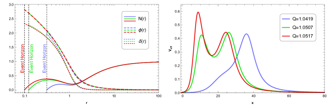
Figure 1: Hairy black hole solutions for $Q=1.0419$ (blue lines), $Q=1.0507$ (green lines) and $Q=1.0517$ (red lines) with $\alpha=0.8$ and the corresponding $l=2$ effective potentials of the scalar field. Left: The metric functions are plotted outside the event horizon (vertical dashed lines), and the solid, dashed and dotted lines designate $N\left(r\right)$, $\phi\left(r\right)$ and $\delta\left(r\right)$, respectively. Right: The effective potentials are displayed against the tortoise coordinate $x$. For a small value of the charge (e.g., the blue line), the effective potential has only a single extremum. As the black hole charge increases (e.g., the green and red lines), the effective potential presents a double-peak structure with two local maxima and one local minimum.

Black hole solutions of the non-linear ordinary differential equations $\left(\ref{eq:NLEqs}\right)$ can be obtained as appropriate boundary conditions at the event horizon $r_{h}$ and the spatial infinity are imposed,

$$m(r_{h}) =r_{h}/2\text{, }\delta(r_{h})=\delta_{0}\text{, }\phi(r_{h})=\phi_{0}\text{, }V(r_{h})=0\text{,}$$

$$m(\infty) =M\text{, }\delta(\infty)=0\text{, }\phi(\infty)=0\text{, }V(\infty)=\Phi\text{,}$$ (4)

where $\Phi$ is the electrostatic potential, and the black hole mass $M$ is related to the ADM mass. The free parameters $\delta_{0}$ and $\phi_{0}$ can be used to characterize different black hole solutions. Specifically, $\phi_{0}=\delta_{0}=0$ lead to the scalar-free solutions with $\phi=0$ of eqn. $\left(\ref{eq:NLEqs}\right)$, which are exactly RN black holes. Nevertheless, hairy black hole solutions with a non-trivial scalar field $\phi$ can exist if non-zero values of $\phi_{0}$ and $\delta_{0}$ are admitted. In this paper, we set $M=1$ and use a shooting method built in the $NDSolve$ function of $Wolfram\text{ }\circledR Mathematica$ to numerically solve eqn. $\left(\ref{eq:NLEqs}\right)$ with the given boundary conditions $\left(\ref{eq:BC}\right)$. The metric functions of three hairy black hole solutions with $\alpha=0.8$ are exhibited in FIG. 1, where the blue, green and red lines denote $Q=1.0419$, $Q=1.0507$ and $Q=1.0517$, respectively.

II.2 Time-dependent Scalar Field Perturbations

For a scalar field perturbation $\delta\phi$ around the hairy black hole, the master equation is given by Herdeiro:2018wub ; Guo:2021enm

$$\left[\nabla^{\mu}\nabla_{\mu}+\left(\alpha+2\alpha^{2}\phi^{2}\left(r\right)\right)\frac{Q^{2}}{r^{4}e^{\alpha\phi^{2}\left(r\right)}}\right]\delta\phi=0.$$ (5)

For later convenience, we define the tortoise coordinate $x$ via $dx/dr\equiv e^{\delta\left(r\right)}N^{-1}\left(r\right)$. The time-dependent scalar field perturbation $\delta\phi$ can be decomposed in terms of spherical harmonics,

$$\delta\phi=\sum_{l,m}\frac{\psi\left(t,r\right)}{r}Y_{lm}\left(\theta,\varphi\right).$$ (6)

With the help of eqns. $\left(\ref{eq:ansatz}\right)$ and $\left(\ref{eq:psi-rt}\right)$, the master equation $\left(\ref{eq:master eq}\right)$ then reduces to

$$\left(-\frac{\partial^{2}}{\partial t^{2}}+\frac{\partial^{2}}{\partial x^{2}}-V_{\text{eff}}\left(x\right)\right)\psi\left(t,x\right)=0,$$ (7)

where the effective potential $V_{\text{eff}}\left(x\right)$ is given by

$$V_{\text{eff}}\left(x\right)=\frac{e^{-2\delta\left(r\right)}N\left(r\right)}{r^{2}}\left[l\left(l+1\right)+1-N\left(r\right)-\frac{Q^{2}}{r^{2}e^{\alpha\phi\left(r\right)^{2}}}-\left(\alpha+2\alpha^{2}\phi\left(r\right)^{2}\right)\frac{Q^{2}}{r^{2}e^{\alpha\phi\left(r\right)^{2}}}\right].$$ (8)

The effective potential with $l=2$ of various black hole solutions is presented in the right panel of FIG. 1. Intriguingly, when the black hole charge is large enough, the effective potential can possess a double-peak structure, which consists of two local maxima and one local minimum.

To solve the partial differential equation $\left(\ref{eq:t-x eq}\right)$, we consider a time-dependent Green’s function $G\left(t,x,x^{\prime}\right)$, which satisfies

$$\left(-\frac{\partial^{2}}{\partial t^{2}}+\frac{\partial^{2}}{\partial x^{2}}-V_{\text{eff}}\left(x\right)\right)G\left(t,x,x^{\prime}\right)=\delta\left(t\right)\delta\left(x-x^{\prime}\right).$$ (9)

One then can express the solution of eqn. $\left(\ref{eq:t-x eq}\right)$ in terms of $G\left(t,x,x^{\prime}\right)$ Andersson:1996cm ; Nollert:1999ji ,

$$\psi\left(t,x\right)=-\int_{-\infty}^{+\infty}\left[G\left(t,x,x^{\prime}\right)\partial_{t}\psi\left(0,x^{\prime}\right)+\partial_{t}G\left(t,x,x^{\prime}\right)\psi\left(0,x^{\prime}\right)\right]dx^{\prime}.$$ (10)

Under the Fourier transformation, the solution $\left(\ref{eq:psi(t,x)-0}\right)$ can be rewritten as

$$\psi\left(t,x\right)=\frac{1}{2\pi}\int_{-\infty}^{+\infty}\hat{G}\left(\omega,x,x^{\prime}\right)\hat{S}\left(\omega,x\right)e^{-i\omega t}dx^{\prime}d\omega,$$ (11)

where $\hat{S}\left(\omega,x\right)$ is determined by the initial data,

$$\hat{S}\left(\omega,x\right)=\left.\left[i\omega\psi\left(t,x\right)-\frac{\partial\psi\left(t,x\right)}{\partial t}\right]\right|_{t=0}.$$ (12)

The time-independent Green’s function $\hat{G}\left(\omega,x,x^{\prime}\right)$ can be constructed in terms of two linearly independent solutions $\hat{\psi}_{-}\left(\omega,x\right)$ and $\hat{\psi}_{+}\left(\omega,x\right)$ to the homogeneous differential equation,

$$\left(\frac{\partial^{2}}{\partial^{2}x}+\omega^{2}-V_{\text{eff}}\left(x\right)\right)\hat{\psi}\left(\omega,x\right)=0,$$ (13)

with the boundary conditions

$$\hat{\psi}_{-}\left(\omega,x\right) \sim e^{-i\omega x},\qquad x\rightarrow-\infty,$$

$$\hat{\psi}_{+}\left(\omega,x\right) \sim e^{i\omega x},\qquad x\rightarrow+\infty.$$ (14)

Particularly, the Green’s function $\hat{G}\left(\omega,x,x^{\prime}\right)$ is given by

$$\hat{G}\left(\omega,x,x^{\prime}\right)=\frac{\hat{\psi}_{-}\left(\omega,\min\left(x,x^{\prime}\right)\right)\hat{\psi}_{+}\left(\omega,\max\left(x,x^{\prime}\right)\right)}{W\left(\omega\right)},$$ (15)

where the Wronskian $W\left(\omega\right)$ is defined as

$$W\left(\omega\right)=\hat{\psi}_{-}\left(\omega,x\right)\partial_{x}\hat{\psi}_{+}\left(\omega,x\right)-\partial_{x}\hat{\psi}_{-}\left(\omega,x\right)\hat{\psi}_{+}\left(\omega,x\right).$$ (16)

When $W\left(\omega\right)=0$, one can infer that $\hat{\psi}_{-}\left(\omega,x\right)$ is identical to $\hat{\psi}_{+}\left(\omega,x\right)$ up to a constant factor, which indicates that $\hat{\psi}_{\pm}\left(\omega,x\right)$ have only ingoing (outgoing) modes at $x=-\infty$ ($x=+\infty$). Therefore, the condition $W\left(\omega\right)=0$ selects a discrete set of quasinormal modes with complex quasinormal frequencies $\omega_{n}$, where $n=0,1,2\ldots$ is the overtone number.

On the complex plane, the solution $\psi\left(t,x\right)$ to eqn. $\left(\ref{eq:t-x eq}\right)$ can be expressed as a sum of quasinormal modes Nollert:1999ji ,

$$\psi\left(t,x\right)=\sum_{n}\psi_{n}\left(t,x\right)=\sum_{n}c_{n}\left(x\right)e^{-i\omega_{n}t},$$ (17)

where the coefficient $c_{n}\left(x\right)$ is

$$c_{n}\left(x\right)=\frac{-i}{dW\left(\omega_{n}\right)/d\omega}\int_{-\infty}^{+\infty}\hat{\psi}_{-}\left(\omega_{n},\min\left(x,x^{\prime}\right)\right)\hat{\psi}_{+}\left(\omega_{n},\max\left(x,x^{\prime}\right)\right)\hat{S}\left(\omega_{n},x^{\prime}\right)dx^{\prime}.$$ (18)

Since the quasinormal modes come in complex conjugate pairs, the waveform $\psi\left(t,x\right)$ given by eqn. $\left(\ref{eq:psi of QNMs}\right)$ is real as long as the initial data $\hat{S}\left(\omega_{n},x\right)$ is real Nollert:1999ji . Note that, before the initial data is entirely received by the observer, a time-dependent integration domain in eqns. $\left(\ref{eq:psi(t,x)-0}\right)$ and $\left(\ref{eq:cn}\right)$ is required to respect causality. Therefore, to well describe the behavior of $\psi\left(t,x\right)$ at a early time, the coefficients $c_{n}\left(x\right)$ are argued to depend on time Andersson:1996cm ; Nollert:1999ji . Nevertheless, we focus on the late-time waveforms throughout this paper, and hence the coefficients $c_{n}\left(x\right)$ are time-independent.

When the real parts of quasinormal frequencies $\omega_{n}$ are an arithmetic progression with regard to the number $n$,

$$\operatorname{Re}\omega_{n}=\omega_{0}+\frac{2n\pi}{T},$$ (19)

the waveform $\psi\left(t,x\right)$ from eqn. $\left(\ref{eq:psi of QNMs}\right)$ with real initial data then behaves as

$$\psi\left(t,x\right)=\sum_{n}\psi_{n}\left(t,x\right)=2\sum_{n}\left[\operatorname{Re}c_{n}\cos\left(\omega_{0}+2n\pi/T\right)t+\operatorname{Im}c_{n}\sin\left(\omega_{0}+2n\pi/T\right)t\right]e^{\operatorname{Im}\omega_{n}t},$$ (20)

where each quasinormal mode $\psi_{n}\left(t,x\right)$ is composed of a complex conjugate pair,

$$\psi_{n}\left(t,x\right)=c_{n}\left(x\right)e^{-i\omega_{n}t}+c_{n}^{\ast}\left(x\right)e^{-i(-\omega_{n}^{\ast})t}.$$ (21)

Interestingly, the waveform $\psi\left(t,x\right)$ describes damped oscillations with a period $T$ and damping factors, which are the imaginary parts of quasinormal modes. As demonstrated in Bueno:2017hyj , the inner barrier of a double-peak potential provides a reflecting wall for radiation waves, leading to a set of quasinormal modes in the form of eqn. $\left(\ref{eq:AP modes}\right)$. Consequently, a distant observer can detect a series of echoes from a double-peak effective potential.

III Numerical Results

In this section, we investigate the waveform $\psi\left(t,x\right)$ detected by a distant observer in the hairy black holes with the effective potential of different peak structure. To numerically solve the partial differential equation $\left(\ref{eq:t-x eq}\right)$, we consider the initial condition,

$$\left.\psi\left(t,x\right)\right|_{t=0}=0\text{ and}\left.\frac{\partial\psi\left(t,x\right)}{\partial t}\right|_{t=0}=A\text{exp}\left(-\frac{\left(x-x_{0}\right)^{2}}{2\Delta^{2}}\right)\text{ \cite[cite]{\@@bibref{Authors Phrase1YearPhrase2}{Cardoso:2016oxy,Cardoso:2017njb,Cardoso:2019rvt}{\@@citephrase{(}}{\@@citephrase{)}}}}.$$ (22)

In the following numerical simulations, the initial position of the Gaussian wave packet $x_{0}$ is placed near the (outer) peak of the effective potential, and the amplitude $A$ and the width $\Delta$ are chosen to adapt to the specific case. To check our numerical results and find the frequency content of $\psi\left(t,x\right)$, we use eqns. $\left(\ref{eq:psi of QNMs}\right)$ and $\left(\ref{eq:cn}\right)$ to reconstruct the waveform $\psi\left(t,x\right)$ at late times from the quasinormal modes. Moreover, we focus on the spherical harmonics of $l=2$ since they play a dominant role in the ringdown gravitational waves after binary black holes merge Giesler:2019uxc ; Sago:2021gbq .

III.1 Single-peak Potential

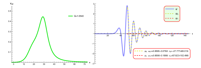
Figure 2: Left: The $l=2$ effective potential of the hairy black hole with $\alpha=0.9$ and $Q=1.0540$ as a function of the tortoise coordinate $x$. The effective potential has a single-peak structure. Right: The waveform $\psi$ (blue solid line), and the first and second lowest-lying quasinormal modes $\psi_{0}$ (yellow dashed line) and $\psi_{1}$ (red dashed line) received by an observer at $x_{\text{o}}=72.75$. The initial condition is the Gaussian perturbation $\left(\ref{eq:initial data}\right)$ near the peak. The fundamental mode $\psi_{0}$ dominates the late-time behavior of the waveform $\psi$.

As shown in FIG. 1, the $l=2$ effective potential of scalar field perturbations has a single-peak structure when the black hole charge is small enough. In FIG. 2, we present the evolution of a time-dependent scalar perturbation in the hairy black hole with $\alpha=0.9$ and $Q=1.0540$. The $l=2$ effective potential is plotted in the left panel, which indeed shows a single-peak structure. In the right panel, we display the waveform signal received by an observer at $x_{\text{o}}=72.75$, who is far away from the potential peak. Specifically, the blue solid line denotes the solution $\psi(t,x_{\text{o}})$ to the partial differential equation $\left(\ref{eq:t-x eq}\right)$ with the initial condition $\left(\ref{eq:initial data}\right)$, and the dashed lines represent the low-lying quasinormal modes $\psi_{0}(t,x_{\text{o}})$ and $\psi_{1}(t,x_{\text{o}})$ obtained from eqns. $\left(\ref{eq:psi of QNMs}\right)$, $\left(\ref{eq:cn}\right)$ and $\left(\ref{eq:initial data}\right)$. Here, we consider the quasinormal modes $\psi_{0}(t,x_{\text{o}})$ and $\psi_{1}(t,x_{\text{o}})$ only after the initial data is fully received by the observer. The right panel of FIG. 2 displays that, roughly after the travel time of the initial data from the vicinity of the peak to the observer, the reflection from the potential peak gives an observed burst, which can be accurately reconstructed from $\psi_{0}$ and $\psi_{1}$. At late times, the wave signal is dominated by the fundamental quasinormal mode $\psi_{0}$, showing an exponentially damped sinusoid. As expected, due to the absence of the inner peak, no echo is observed after the burst is received. Note that waves propagating on a black hole spacetime usually develop asymptotically late-time tails, which follow exponentially damped sinusoids and decay as an inverse power of time due to scattering from large radius in the black hole geometry Price:1972pw ; Ching:1994bd . Nevertheless, discussions on the power-law tails are beyond the scope of the paper.

III.2 Wormhole-like Potential

For a large enough black hole charge, there can exist two peaks in the effective potential of scalar field perturbations. Depending on the black hole parameters, the separation between the peaks $L$ can be considerably larger than the Compton wavelength of the scalar field perturbations (or the wavelength of the associated quasinormal modes), which resembles the usual wormhole spacetime. Since the potential peaks are well separated, the scattering of a perturbation off one peak is barely influenced by the other one. The perturbation is reflected off the potential barriers, and bounces back and forth between the two peaks. Meanwhile, the perturbation successively tunnels through the outer barrier, leading to a series of echoes received by a distant observer. In this case, the geometric optics approximation is valid, and hence the time delay between the echoes is roughly $2L$. For a detail discussion, one can refer to Mark:2017dnq ; Bueno:2017hyj . As noted in Bueno:2017hyj , the appearance of echoes in a double-peak potential is closely related to quasinormal modes residing in the valley between the peaks. When the distance between the peaks is much larger than the width of the peaks, there exists a series of these quasinormal modes, whose imaginary parts are much smaller than their real parts. Similar to a beat produced by multiple sounds of slightly different frequencies, the superposition of the quasinormal modes, which leak through the outer potential barrier, produce approximately periodical echo signals.

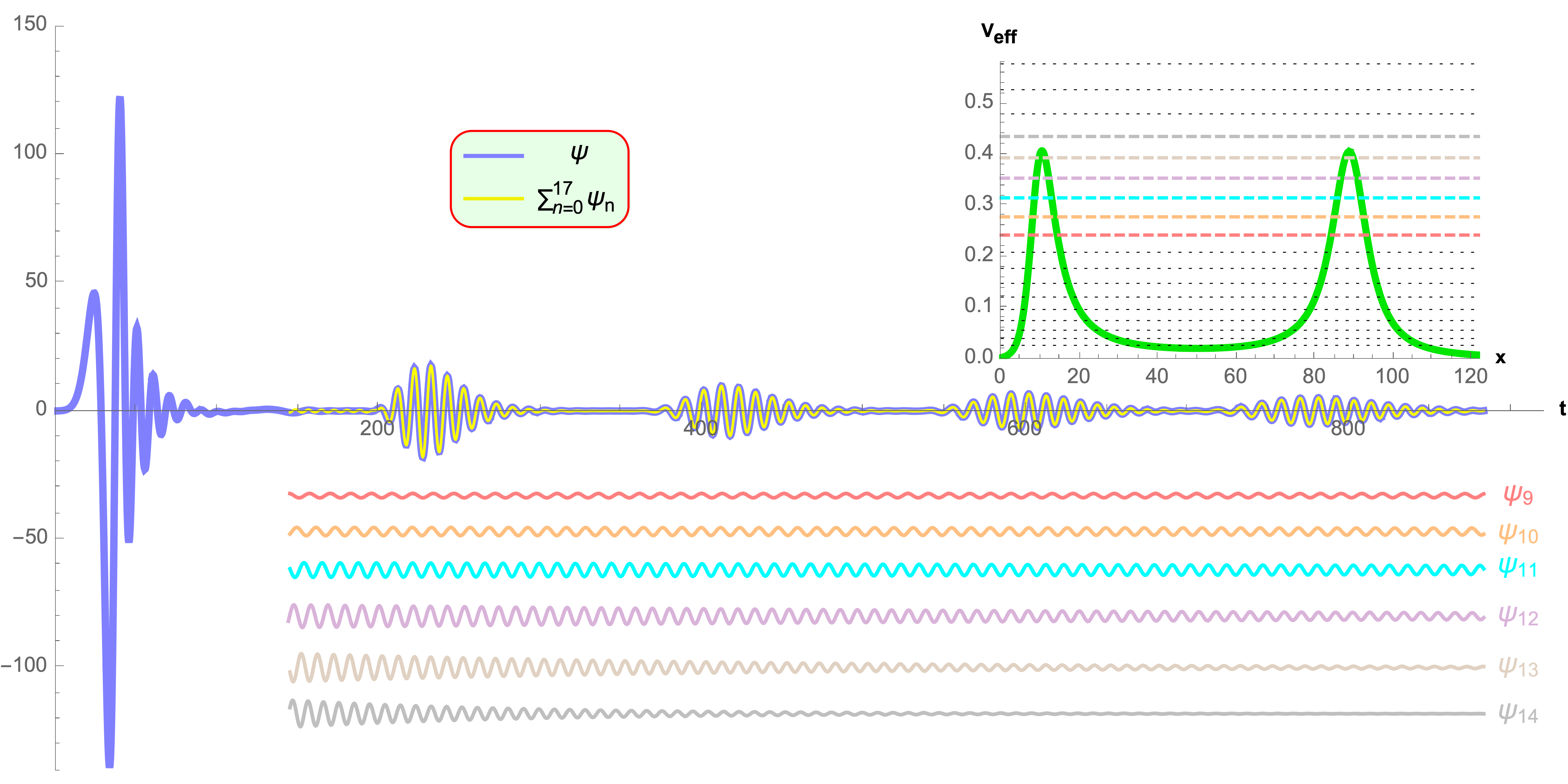
Figure 3: The upper-right inset shows the $l=2$ effective potential of two well-separated peaks in the hairy black hole with $\alpha=0.52$ and $Q=1.0074$. The blue line denotes the observed time signal, which is obtained from numerical integration of eqn. $\left(\ref{eq:t-x eq}\right)$ with an initial Gaussian’s packet near the outer peak. We take the observer to be sufficiently far away from the outer peak. Due to the double-peak structure, a sequence of echoes starts to appear after the primary signal, and can be well reconstructed from the quasinormal modes from $n=0$ to $n=17$ (yellow line). Below the time axis, we exhibit the waveform of the quasinormal modes from $n=9$ to $n=14$ individually, which dominate the reconstruction of the echoes. Additionally, $\left(\operatorname{Re}\omega_{n}\right)^{2}$ of the quasinormal modes are plotted as horizontal lines in the inset. The smaller $n$ is, the lower the horizontal line lies.

In FIG. 3, we present the numerically computed and reconstructed time signals received by an observer far away from the outer peak of the effective potential in the hairy black hole with $\alpha=0.52$ and $Q=1.0074$. The blue line designates the numerical solution $\psi\left(t,x\right)$ to the partial differential equation $\left(\ref{eq:t-x eq}\right)$, while the yellow line represents the sum over the associated quasinormal modes from $n=0$ to $n=17$. One can observe that a series of echoes roughly separated by a distance $2L\approx$ $156.68$ arises at late times, and the sum of quasinormal modes perfectly reconstruct the echoes. In TABLE 1, we list the quasinormal frequency $\omega_{n}$ and the corresponding coefficient $c_{n}$ for each quasinormal mode $\psi_{n}$. Roughly speaking, these quasinormal frequencies $\omega_{n}$ satisfy the form in eqn. $\left(\ref{eq:AP modes}\right)$ with a period $T\approx 179.52\sim 2L$, which is consistent with the echo period. To illustrate the contributions from quasinormal modes, the dominant modes $\psi_{9}\sim\psi_{14}$ are individually exhibited below the time axis of FIG. 3. Moreover, the squares of the real parts of the quasinormal frequencies $\left(\operatorname{Re}\omega_{n}\right)^{2}$ are displayed as horizontal lines in the upper-right inset. The dashed lines represent the dominant modes with the same colors as those below the time axis, while the dotted lines denote other quasinormal modes. The quasinormal modes spread out beyond the potential valley by penetrating the potential barriers. It shows that, the smaller $n$ is, the closer the quasinormal mode lives to the bottom of the valley, thus making it penetrate the potential barriers more difficult. Note that the coefficients $c_{n}$ are strongly related to the transmission of the scalar perturbation penetrating the outer barrier, which implies that low-lying quasinormal modes have small values of $c_{n}$. For the quasinormal modes $\psi_{n<9}$, the coefficients $c_{n<9}$ are so small that their contributions to the echoes can be neglected. On the other hand, the frequency of the high-lying modes $\psi_{n>14}$ attains a large negative imaginary part, providing a prominent exponentially damping factor for the time signal.

Table 1: The frequency $\omega_{n}$ of the quasinormal modes of $l=2$ for a scalar field perturbation in the hairy black hole with $\alpha=0.52$ and $Q=1.0074$. The coefficient $c_{n}$, which controls the contribution from the corresponding quasinormal mode to the echoes in FIG. 3, is obtained from eqn. $\left(\ref{eq:cn}\right)$. As $n$ grows, the modulus of $c_{n}$ becomes larger. Since the initial data is real, each pair of coefficients $c_{n}$ are complex conjugate, leading to the real waveform of the quasinormal modes $\psi_{n}$.

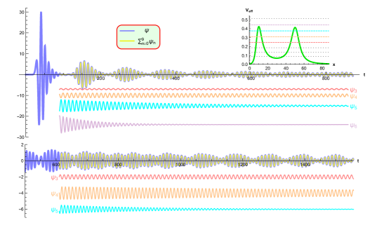
Figure 4: Exact numerical (blue lines) and reconstructed (yellow lines) waveforms $\psi$, and the dominant quasinormal modes received by a distant observer in the hairy black hole with $\alpha=0.6$ and $Q=1.0192$. Compared to FIG. 3, the effective potential has a smaller valley between two peaks, leading to fewer quasinormal modes (see horizontal lines, representing $\left(\operatorname{Re}\omega_{n}\right)^{2}$ of quasinormal modes, in the inset). In the upper panel, the echoes are observed after the primary signal and disappear after some time. The lower panel shows the later behavior of the waveform. Interestingly, the echoes reoccur after the quasinormal mode $\psi_{5}$ is damped away. Specifically, the superposition of the quasinormal modes $\psi_{3}$ and $\psi_{4}$ produce the reoccurring echoes at the later time.

In FIG. 4, we display the numerically computed and reconstructed waveforms at a position far away from the outer peak in the hairy black hole solution with $\alpha=0.6$ and $Q=1.0192$, where the effective potential has a smaller valley than that of FIG. 3. In addition, the dominant quasinormal modes of the waveform $\psi$ are also exhibited below the time axis. Unlike FIG. 3, we observe that there exists a time regime (roughly between $700$ and $1000$), in which echoes overlaps, and echo signals can be hardly identified. Interestingly, after the quasinormal mode $\psi_{5}$ becomes negligible, the echoes composed of the low-lying modes $\psi_{3}$ and $\psi_{4}$ reappear. Moreover, the frequency $\omega_{n}$ and the coefficient $c_{n}$ of the quasinormal modes $\psi_{n\leq 9}$ are given in TABLE 2. Compared to FIG. 3 and TABLE 1, we find that fewer quasinormal modes are available to reconstruct the waveform due to a smaller potential valley Guo:2021enm . In fact, as shown in the inset of FIG. 4, the quasinormal modes get farther apart as the potential valley becomes narrower and shallower.

Table 2: The frequency $\omega_{n}$ and the coefficient $c_{n}$ of the quasinormal modes of $l=2$ for a scalar field perturbation in the hairy black hole with $\alpha=0.6$ and $Q=1.0192$. Compared to TABLE 1, fewer quasinormal modes are available to reconstruct the waveform in FIG. 4.

III.3 Adjacent Double-peak Potential

Finally, we consider the hairy black hole solutions with the double-peak effective potential, where the separation between the peaks $L$ is comparable to the Compton wavelength of the perturbations. Unlike the wormhole-like potential, the geometric optics approximation fails, and hence the time delay between the echoes can be larger than $2L$. Furthermore, albeit there always exist long-lived modes trapped at the potential valley, the number of the long-lived modes decreases as $L$ decreases Guo:2021enm . In Guo:2021enm , we also found that, near the smaller local maximum of the potential, there appear sub-long-lived modes, which could play an important role in the late-time waveform when the contribution from the long-lived modes is suppressed by their small tunneling rates through the potential barriers.

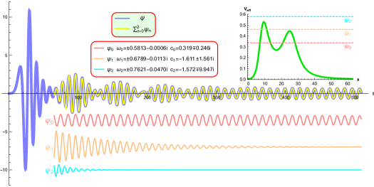
Figure 5: Numerical (blue line) and reconstructed (yellow line) waveforms $\psi$ excited by a Gaussian perturbation near the outer potential peak in the hairy black hole with $\alpha=0.8$ and $Q=1.0514$. The observer is far away from the outer peak. Compared to FIGs. 3 and 4, the effective potential has a significantly shallower and narrower valley. Therefore, only three quasinormal modes, namely $\psi_{0}$, $\psi_{1}$ and $\psi_{2}$, are needed to reconstruct the waveform after the primary signal is received. The superposition of these quasinormal modes leads to the observed echoes. Moreover, since the geometric optics approximation is invalid, the time delay between the echoes is obtained from the real parts of the quasinormal frequencies instead of the distance between the peaks. The dashed horizontal lines in the inset represent $\left(\operatorname{Re}\omega_{n}\right)^{2}$ of $\psi_{0}$, $\psi_{1}$ and $\psi_{2}$, indicating that $\psi_{0}$ is trapped near the bottom of the potential valley and therefore a long-lived mode. After $\psi_{1}$ and $\psi_{2}$ are damped away, the waveform $\psi$ is only determined by the long-lived mode $\psi_{0}$, and hence has a sinusoid tail instead of echoes.

In FIG. 5, we investigate the waveform of a scalar perturbation propagating in the double-peak effective potential of the hairy black hole with $\alpha=0.8$ and $Q=1.0514$, where the inner barrier is higher than the outer one. After the primary signal, one observes three distinct echoes followed by an apparent sinusoid. Since a shallow potential valley gives rise to fewer quasinormal modes Guo:2021enm , the late-time waveform $\psi$ can be well reconstructed by only three lowest-lying modes $\psi_{n\leq 2}$. Moreover, one can read off the echo period $T\approx 64.38$ from the quasinormal frequencies $\omega_{0}$, $\omega_{1}$ and $\omega_{2}$ via eqn. $\left(\ref{eq:AP modes}\right)$. Therefore, the echoes are separated by a distance $T\approx 64.38$, which is larger than $2L\approx 31.10$. In the inset, $\left(\operatorname{Re}\omega_{n}\right)^{2}$ of the the quasinormal modes $\psi_{n\leq 2}$ are displayed as dashed horizontal lines. It shows that the $n=0$ quasinormal mode lives at the bottom of the potential valley and is a long-lived state with a very small imaginary part of the quasinormal frequency. Additionally, $\psi_{1}$ is a sub-long-lived mode that lives near the smaller local maximum of the double-peak potential. The superposition of $\psi_{0}$, $\psi_{1}$ and $\psi_{2}$ generates the first echo, whereas the following echoes are mainly determined by $\psi_{0}$ and $\psi_{1}$. After the echo signals, only the long-lived mode $\psi_{0}$ remains, which results in a long sinusoid tail. It is worth emphasizing that the amplitude of the tail is much larger than that in the single-peak case since the imaginary part of $\omega_{0}$ is roughly $100$ times smaller.

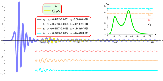
Figure 6: Numerical (blue line) and reconstructed (yellow line) waveforms $\psi$ excited by a Gaussian perturbation near the outer potential peak in the hairy black hole with $\alpha=0.7$ and $Q=1.0340$, which has a higher outer potential barrier than in FIG. 5. The higher outer potential barrier reduces the transmission rate of the perturbation through the barrier. As a result, the long-lived mode $\psi_{0}$ is negligible, and the sub-long-lived mode $\psi_{1}$ trapped at the smaller local maximum of the potential determines the late-time sinusoid tail, which has a much smaller amplitude and a large decay rate than that in FIG. 5. In addition, there appears only one distinguishable echo, which mainly consists of the quasinormal modes $\psi_{1}$, $\psi_{2}$ and $\psi_{3}$.

To illustrate the effect of the outer potential barrier on the received signals, we consider the hairy black hole with $\alpha=0.7$ and $Q=1.0340$, whose effective potential has a higher outer potential barrier than that in FIG. 5. In fact, as the height of the outer potential barrier increases, perturbations escape from the potential valley to a distant observer more difficultly. As expected, FIG. 6 shows that the late time signal detected by a distant observer is dimmer than that in FIG. 5. Specifically, the dashed horizontal lines in the inset indicate that the quasinormal modes $\psi_{0}$ and $\psi_{1}$ are long-lived and sub-long-lived modes trapped at the minimum and the smaller local maximum of the potential, respectively. Due to the small transmission rate through the high outer barrier, the long-lived mode $\psi_{0}$ has the negligibly small coefficient $c_{0}$ and thus contributes little to the late-time signal. Consequently, the late-time waveform is primarily controlled by the sub-long-lived mode $\psi_{1}$, which has smaller modulus of the coefficient $c_{1}$ and decays faster than the long-lived mode $\psi_{0}$ in FIG. 5, hence leading to fewer echoes and a smaller sinusoid tail.

IV Conclusions

In this paper, we first studied hairy black holes in the EMS model, where the scalar field is minimally coupled to the gravity sector and non-minimally coupled to the electromagnetic field. It showed that the effective potential of scalar perturbations can possess a single peak or two peaks depending on the black hole parameters. Moreover, for the double-peak potential, the separation between the peaks can be significantly larger or comparable to the Compton wavelength of the perturbations. Considering an initial Gaussian perturbation near the (outer) potential peak, the evolution of the time-dependent scalar perturbation was then computed in several hairy black holes to investigate how the peak structure affects the late-time waveform of the perturbation received by an observer far away from the (outer) peak. Specifically, the waveform was obtained by numerically solving the partial differential equation $\left(\ref{eq:t-x eq}\right)$. To find the frequency content of the waveform, we also used eqn. $\left(\ref{eq:psi of QNMs}\right)$ to reconstruct the waveform with the associated quasinormal modes. Our results showed that the numerical and reconstructed waveforms are in excellent agreement.

After relaxation of the initial perturbation, the observer first detects a primary signal, which is the reflected wave off the (outer) potential peak and hence essentially controlled by the quasinormal modes associated with the (outer) peak. If there is no inner peak, the late-time waveform after the primary signal is an exponentially decaying sinusoid, which is the fundamental quasinormal mode. On the other hand, the late-time waveform in a double-peak potential is mostly determined by the long-lived and sub-long-lived quasinormal modes, which live near the minimum and the smaller local maximum of the potential, respectively. When the distance between the peaks is large, there exist a number of long-lived and sub-long-lived modes, which produce a train of decaying echo pulses observed in FIGs. 3 and 4. Remarkably, if the number of long-lived modes is small enough, echo signals can disappear for some time and then reappear (see FIG. 4). When the potential peaks are close enough, there exist only one long-lived mode and one sub-long-lived mode. The superposition of the long-lived, sub-long-lived and other low-lying modes give a few observed echoes following the primary signal (see FIGs. 5 and 6). For a low outer potential barrier, the long-lived mode dominates the waveform of the perturbation after other modes are damped away, producing a very slowly decaying sinusoid tail (see FIG. 5). For a high outer potential barrier, the long-lived mode is suppressed, and the sub-long-lived is then responsible for the sinusoid tail of the waveform, which decays faster and has a much smaller amplitude (see FIG. 6).

For spherically symmetric hairy black holes, the connection between double-peak effective potentials and the existence of multiple photon spheres outside the event horizon has been discussed in Guo:2021enm . The late-time waveform excited by a scalar perturbation may provide a smoking gun for the detection of black holes with multiple photon spheres. It will be of great interest if our analysis can be generalized beyond spherical symmetry and for more general black hole spacetimes.

- (1) B.P. Abbott et al. Observation of Gravitational Waves from a Binary Black Hole Merger. Phys. Rev. Lett., 116(6):061102, 2016. arXiv:1602.03837, doi:10.1103/PhysRevLett.116.061102.
- (2) Kazunori Akiyama et al. First M87 Event Horizon Telescope Results. I. The Shadow of the Supermassive Black Hole. Astrophys. J. Lett., 875:L1, 2019. arXiv:1906.11238, doi:10.3847/2041-8213/ab0ec7.
- (3) Kazunori Akiyama et al. First M87 Event Horizon Telescope Results. II. Array and Instrumentation. Astrophys. J. Lett., 875(1):L2, 2019. arXiv:1906.11239, doi:10.3847/2041-8213/ab0c96.
- (4) Kazunori Akiyama et al. First M87 Event Horizon Telescope Results. III. Data Processing and Calibration. Astrophys. J. Lett., 875(1):L3, 2019. arXiv:1906.11240, doi:10.3847/2041-8213/ab0c57.
- (5) Kazunori Akiyama et al. First M87 Event Horizon Telescope Results. IV. Imaging the Central Supermassive Black Hole. Astrophys. J. Lett., 875(1):L4, 2019. arXiv:1906.11241, doi:10.3847/2041-8213/ab0e85.
- (6) Kazunori Akiyama et al. First M87 Event Horizon Telescope Results. V. Physical Origin of the Asymmetric Ring. Astrophys. J. Lett., 875(1):L5, 2019. arXiv:1906.11242, doi:10.3847/2041-8213/ab0f43.
- (7) Kazunori Akiyama et al. First M87 Event Horizon Telescope Results. VI. The Shadow and Mass of the Central Black Hole. Astrophys. J. Lett., 875(1):L6, 2019. arXiv:1906.11243, doi:10.3847/2041-8213/ab1141.
- (8) Hans-Peter Nollert. TOPICAL REVIEW: Quasinormal modes: the characteristic ‘sound’ of black holes and neutron stars. Class. Quant. Grav., 16:R159–R216, 1999. doi:10.1088/0264-9381/16/12/201.
- (9) Emanuele Berti, Vitor Cardoso, Jose A. Gonzalez, and Ulrich Sperhake. Mining information from binary black hole mergers: A Comparison of estimation methods for complex exponentials in noise. Phys. Rev. D, 75:124017, 2007. arXiv:gr-qc/0701086, doi:10.1103/PhysRevD.75.124017.
- (10) Vitor Cardoso, Edgardo Franzin, and Paolo Pani. Is the gravitational-wave ringdown a probe of the event horizon? Phys. Rev. Lett., 116(17):171101, 2016. [Erratum: Phys.Rev.Lett. 117, 089902 (2016)]. arXiv:1602.07309, doi:10.1103/PhysRevLett.116.171101.
- (11) Richard H. Price and Gaurav Khanna. Gravitational wave sources: reflections and echoes. Class. Quant. Grav., 34(22):225005, 2017. arXiv:1702.04833, doi:10.1088/1361-6382/aa8f29.
- (12) Matthew Giesler, Maximiliano Isi, Mark A. Scheel, and Saul Teukolsky. Black Hole Ringdown: The Importance of Overtones. Phys. Rev. X, 9(4):041060, 2019. arXiv:1903.08284, doi:10.1103/PhysRevX.9.041060.
- (13) Jose P. S. Lemos and Oleg B. Zaslavskii. Black hole mimickers: Regular versus singular behavior. Phys. Rev. D, 78:024040, 2008. arXiv:0806.0845, doi:10.1103/PhysRevD.78.024040.
- (14) Pedro V. P. Cunha, José A. Font, Carlos Herdeiro, Eugen Radu, Nicolas Sanchis-Gual, and Miguel Zilhão. Lensing and dynamics of ultracompact bosonic stars. Phys. Rev. D, 96(10):104040, 2017. arXiv:1709.06118, doi:10.1103/PhysRevD.96.104040.
- (15) Pedro V. P. Cunha and Carlos A. R. Herdeiro. Shadows and strong gravitational lensing: a brief review. Gen. Rel. Grav., 50(4):42, 2018. arXiv:1801.00860, doi:10.1007/s10714-018-2361-9.
- (16) Rajibul Shaikh, Pritam Banerjee, Suvankar Paul, and Tapobrata Sarkar. A novel gravitational lensing feature by wormholes. Phys. Lett. B, 789:270–275, 2019. [Erratum: Phys.Lett.B 791, 422–423 (2019)]. arXiv:1811.08245, doi:10.1016/j.physletb.2018.12.030.
- (17) De-Chang Dai and Dejan Stojkovic. Observing a Wormhole. Phys. Rev. D, 100(8):083513, 2019. arXiv:1910.00429, doi:10.1103/PhysRevD.100.083513.
- (18) Hyat Huang and Jinbo Yang. Charged Ellis Wormhole and Black Bounce. Phys. Rev. D, 100(12):124063, 2019. arXiv:1909.04603, doi:10.1103/PhysRevD.100.124063.
- (19) John H. Simonetti, Michael J. Kavic, Djordje Minic, Dejan Stojkovic, and De-Chang Dai. Sensitive searches for wormholes. Phys. Rev. D, 104(8):L081502, 2021. arXiv:2007.12184, doi:10.1103/PhysRevD.104.L081502.
- (20) Maciek Wielgus, Jiri Horak, Frederic Vincent, and Marek Abramowicz. Reflection-asymmetric wormholes and their double shadows. Phys. Rev. D, 102(8):084044, 2020. arXiv:2008.10130, doi:10.1103/PhysRevD.102.084044.
- (21) Jinbo Yang and Hyat Huang. Trapping horizons of the evolving charged wormhole and black bounce. Phys. Rev. D, 104(8):084005, 2021. arXiv:2104.11134, doi:10.1103/PhysRevD.104.084005.
- (22) Cosimo Bambi and Dejan Stojkovic. Astrophysical Wormholes. Universe, 7(5):136, 2021. arXiv:2105.00881, doi:10.3390/universe7050136.
- (23) Jun Peng, Minyong Guo, and Xing-Hui Feng. Observational Signature and Additional Photon Rings of Asymmetric Thin-shell Wormhole. 2 2021. arXiv:2102.05488.
- (24) Pablo Bueno, Pablo A. Cano, Frederik Goelen, Thomas Hertog, and Bert Vercnocke. Echoes of Kerr-like wormholes. Phys. Rev. D, 97(2):024040, 2018. arXiv:1711.00391, doi:10.1103/PhysRevD.97.024040.
- (25) R. A. Konoplya, Z. Stuchlík, and A. Zhidenko. Echoes of compact objects: new physics near the surface and matter at a distance. Phys. Rev. D, 99(2):024007, 2019. arXiv:1810.01295, doi:10.1103/PhysRevD.99.024007.
- (26) Yu-Tong Wang, Jun Zhang, and Yun-Song Piao. Primordial gravastar from inflation. Phys. Lett. B, 795:314–318, 2019. arXiv:1810.04885, doi:10.1016/j.physletb.2019.06.036.
- (27) Yu-Tong Wang, Zhi-Peng Li, Jun Zhang, Shuang-Yong Zhou, and Yun-Song Piao. Are gravitational wave ringdown echoes always equal-interval? Eur. Phys. J. C, 78(6):482, 2018. arXiv:1802.02003, doi:10.1140/epjc/s10052-018-5974-y.
- (28) Vitor Cardoso and Paolo Pani. Testing the nature of dark compact objects: a status report. Living Rev. Rel., 22(1):4, 2019. arXiv:1904.05363, doi:10.1007/s41114-019-0020-4.
- (29) José T. Gálvez Ghersi, Andrei V. Frolov, and David A. Dobre. Echoes from the scattering of wavepackets on wormholes. Class. Quant. Grav., 36(13):135006, 2019. arXiv:1901.06625, doi:10.1088/1361-6382/ab23c8.
- (30) Hang Liu, Peng Liu, Yunqi Liu, Bin Wang, and Jian-Pin Wu. Echoes from phantom wormholes. Phys. Rev. D, 103(2):024006, 2021. arXiv:2007.09078, doi:10.1103/PhysRevD.103.024006.
- (31) Min-Yan Ou, Meng-Yun Lai, and Hyat Huang. Echoes from Asymmetric Wormholes and Black Bounce. 11 2021. arXiv:2111.13890.
- (32) Jahed Abedi, Hannah Dykaar, and Niayesh Afshordi. Echoes from the Abyss: Tentative evidence for Planck-scale structure at black hole horizons. Phys. Rev. D, 96(8):082004, 2017. arXiv:1612.00266, doi:10.1103/PhysRevD.96.082004.
- (33) Jahed Abedi, Hannah Dykaar, and Niayesh Afshordi. Echoes from the Abyss: The Holiday Edition! 1 2017. arXiv:1701.03485.
- (34) Ramit Dey, Shauvik Biswas, and Sumanta Chakraborty. Ergoregion instability and echoes for braneworld black holes: Scalar, electromagnetic, and gravitational perturbations. Phys. Rev. D, 103(8):084019, 2021. arXiv:2010.07966, doi:10.1103/PhysRevD.103.084019.
- (35) Yi Yang, Dong Liu, Zhaoyi Xu, Yujia Xing, Shurui Wu, and Zheng-Wen Long. Echoes of novel black-bounce spacetimes. Phys. Rev. D, 104(10):104021, 2021. arXiv:2107.06554, doi:10.1103/PhysRevD.104.104021.
- (36) Sebastian H. Völkel and Kostas D. Kokkotas. Ultra Compact Stars: Reconstructing the Perturbation Potential. Class. Quant. Grav., 34(17):175015, 2017. arXiv:1704.07517, doi:10.1088/1361-6382/aa82de.
- (37) Zachary Mark, Aaron Zimmerman, Song Ming Du, and Yanbei Chen. A recipe for echoes from exotic compact objects. Phys. Rev. D, 96(8):084002, 2017. arXiv:1706.06155, doi:10.1103/PhysRevD.96.084002.
- (38) Qingwen Wang, Naritaka Oshita, and Niayesh Afshordi. Echoes from Quantum Black Holes. Phys. Rev. D, 101(2):024031, 2020. arXiv:1905.00446, doi:10.1103/PhysRevD.101.024031.
- (39) Krishan Saraswat and Niayesh Afshordi. Quantum Nature of Black Holes: Fast Scrambling versus Echoes. JHEP, 04:136, 2020. arXiv:1906.02653, doi:10.1007/JHEP04(2020)136.
- (40) Ramit Dey, Sumanta Chakraborty, and Niayesh Afshordi. Echoes from braneworld black holes. Phys. Rev. D, 101(10):104014, 2020. arXiv:2001.01301, doi:10.1103/PhysRevD.101.104014.
- (41) Naritaka Oshita, Daichi Tsuna, and Niayesh Afshordi. Quantum Black Hole Seismology I: Echoes, Ergospheres, and Spectra. Phys. Rev. D, 102(2):024045, 2020. arXiv:2001.11642, doi:10.1103/PhysRevD.102.024045.
- (42) Sumanta Chakraborty, Elisa Maggio, Anupam Mazumdar, and Paolo Pani. Implications of the quantum nature of the black hole horizon on the gravitational-wave ringdown. 2 2022. arXiv:2202.09111.
- (43) Hang Liu, Wei-Liang Qian, Yunqi Liu, Jian-Pin Wu, Bin Wang, and Rui-Hong Yue. Alternative mechanism for black hole echoes. Phys. Rev. D, 104(4):044012, 2021. arXiv:2104.11912, doi:10.1103/PhysRevD.104.044012.
- (44) Kabir Chakravarti, Rajes Ghosh, and Sudipta Sarkar. Signature of nonuniform area quantization on black hole echoes. Phys. Rev. D, 105(4):044046, 2022. arXiv:2112.10109, doi:10.1103/PhysRevD.105.044046.
- (45) Guido D’Amico and Nemanja Kaloper. Black hole echoes. Phys. Rev. D, 102(4):044001, 2020. arXiv:1912.05584, doi:10.1103/PhysRevD.102.044001.
- (46) Hai-Shan Liu, Zhan-Feng Mai, Yue-Zhou Li, and H. Lü. Quasi-topological Electromagnetism: Dark Energy, Dyonic Black Holes, Stable Photon Spheres and Hidden Electromagnetic Duality. Sci. China Phys. Mech. Astron., 63:240411, 2020. arXiv:1907.10876, doi:10.1007/s11433-019-1446-1.
- (47) Hyat Huang, Min-Yan Ou, Meng-Yun Lai, and H. Lu. Echoes from Classical Black Holes. 12 2021. arXiv:2112.14780.
- (48) Claudia de Rham, Gregory Gabadadze, and Andrew J. Tolley. Resummation of Massive Gravity. Phys. Rev. Lett., 106:231101, 2011. arXiv:1011.1232, doi:10.1103/PhysRevLett.106.231101.
- (49) Ruifeng Dong and Dejan Stojkovic. Gravitational wave echoes from black holes in massive gravity. Phys. Rev. D, 103(2):024058, 2021. arXiv:2011.04032, doi:10.1103/PhysRevD.103.024058.
- (50) Carlos A.R. Herdeiro, Eugen Radu, Nicolas Sanchis-Gual, and José A. Font. Spontaneous Scalarization of Charged Black Holes. Phys. Rev. Lett., 121(10):101102, 2018. arXiv:1806.05190, doi:10.1103/PhysRevLett.121.101102.
- (51) R. A. Konoplya and A. Zhidenko. Analytical representation for metrics of scalarized Einstein-Maxwell black holes and their shadows. Phys. Rev. D, 100(4):044015, 2019. arXiv:1907.05551, doi:10.1103/PhysRevD.100.044015.
- (52) Peng Wang, Houwen Wu, and Haitang Yang. Scalarized Einstein-Born-Infeld-scalar Black Holes. 12 2020. arXiv:2012.01066.
- (53) Guangzhou Guo, Peng Wang, Houwen Wu, and Haitang Yang. Scalarized Einstein–Maxwell-scalar black holes in anti-de Sitter spacetime. Eur. Phys. J. C, 81(10):864, 2021. arXiv:2102.04015, doi:10.1140/epjc/s10052-021-09614-7.
- (54) Guangzhou Guo, Peng Wang, Houwen Wu, and Haitang Yang. Thermodynamics and Phase Structure of an Einstein-Maxwell-scalar Model in Extended Phase Space. 7 2021. arXiv:2107.04467.
- (55) Werner Israel. Event horizons in static vacuum space-times. Phys. Rev., 164:1776–1779, 1967. doi:10.1103/PhysRev.164.1776.
- (56) B. Carter. Axisymmetric Black Hole Has Only Two Degrees of Freedom. Phys. Rev. Lett., 26:331–333, 1971. doi:10.1103/PhysRevLett.26.331.
- (57) Remo Ruffini and John A. Wheeler. Introducing the black hole. Phys. Today, 24(1):30, 1971. doi:10.1063/1.3022513.
- (58) Pedro G. S. Fernandes, Carlos A. R. Herdeiro, Alexandre M. Pombo, Eugen Radu, and Nicolas Sanchis-Gual. Spontaneous Scalarisation of Charged Black Holes: Coupling Dependence and Dynamical Features. Class. Quant. Grav., 36(13):134002, 2019. [Erratum: Class.Quant.Grav. 37, 049501 (2020)]. arXiv:1902.05079, doi:10.1088/1361-6382/ab23a1.
- (59) Pedro G.S. Fernandes, Carlos A.R. Herdeiro, Alexandre M. Pombo, Eugen Radu, and Nicolas Sanchis-Gual. Charged black holes with axionic-type couplings: Classes of solutions and dynamical scalarization. Phys. Rev. D, 100(8):084045, 2019. arXiv:1908.00037, doi:10.1103/PhysRevD.100.084045.
- (60) Jose Luis Blázquez-Salcedo, Carlos A.R. Herdeiro, Jutta Kunz, Alexandre M. Pombo, and Eugen Radu. Einstein-Maxwell-scalar black holes: the hot, the cold and the bald. Phys. Lett. B, 806:135493, 2020. arXiv:2002.00963, doi:10.1016/j.physletb.2020.135493.
- (61) De-Cheng Zou and Yun Soo Myung. Scalarized charged black holes with scalar mass term. Phys. Rev. D, 100(12):124055, 2019. arXiv:1909.11859, doi:10.1103/PhysRevD.100.124055.
- (62) Pedro G.S. Fernandes. Einstein-Maxwell-scalar black holes with massive and self-interacting scalar hair. Phys. Dark Univ., 30:100716, 2020. arXiv:2003.01045, doi:10.1016/j.dark.2020.100716.
- (63) Yan Peng. Scalarization of horizonless reflecting stars: neutral scalar fields non-minimally coupled to Maxwell fields. Phys. Lett. B, 804:135372, 2020. arXiv:1912.11989, doi:10.1016/j.physletb.2020.135372.
- (64) Yun Soo Myung and De-Cheng Zou. Instability of Reissner–Nordström black hole in Einstein-Maxwell-scalar theory. Eur. Phys. J. C, 79(3):273, 2019. arXiv:1808.02609, doi:10.1140/epjc/s10052-019-6792-6.
- (65) Yun Soo Myung and De-Cheng Zou. Stability of scalarized charged black holes in the Einstein–Maxwell–Scalar theory. Eur. Phys. J. C, 79(8):641, 2019. arXiv:1904.09864, doi:10.1140/epjc/s10052-019-7176-7.
- (66) De-Cheng Zou and Yun Soo Myung. Radial perturbations of the scalarized black holes in Einstein-Maxwell-conformally coupled scalar theory. Phys. Rev. D, 102(6):064011, 2020. arXiv:2005.06677, doi:10.1103/PhysRevD.102.064011.
- (67) Yun Soo Myung and De-Cheng Zou. Onset of rotating scalarized black holes in Einstein-Chern-Simons-Scalar theory. Phys. Lett. B, 814:136081, 2021. arXiv:2012.02375, doi:10.1016/j.physletb.2021.136081.
- (68) Zhan-Feng Mai and Run-Qiu Yang. Stability analysis on charged black hole with non-linear complex scalar. 12 2020. arXiv:2101.00026.
- (69) Dumitru Astefanesei, Carlos Herdeiro, João Oliveira, and Eugen Radu. Higher dimensional black hole scalarization. JHEP, 09:186, 2020. arXiv:2007.04153, doi:10.1007/JHEP09(2020)186.
- (70) Yun Soo Myung and De-Cheng Zou. Quasinormal modes of scalarized black holes in the Einstein–Maxwell–Scalar theory. Phys. Lett. B, 790:400–407, 2019. arXiv:1812.03604, doi:10.1016/j.physletb.2019.01.046.
- (71) Jose Luis Blázquez-Salcedo, Carlos A.R. Herdeiro, Sarah Kahlen, Jutta Kunz, Alexandre M. Pombo, and Eugen Radu. Quasinormal modes of hot, cold and bald Einstein-Maxwell-scalar black holes. 8 2020. arXiv:2008.11744.
- (72) Yun Soo Myung and De-Cheng Zou. Scalarized charged black holes in the Einstein-Maxwell-Scalar theory with two U(1) fields. Phys. Lett. B, 811:135905, 2020. arXiv:2009.05193, doi:10.1016/j.physletb.2020.135905.
- (73) Yun Soo Myung and De-Cheng Zou. Scalarized black holes in the Einstein-Maxwell-scalar theory with a quasitopological term. Phys. Rev. D, 103(2):024010, 2021. arXiv:2011.09665, doi:10.1103/PhysRevD.103.024010.
- (74) Hong Guo, Xiao-Mei Kuang, Eleftherios Papantonopoulos, and Bin Wang. Topology and spacetime structure influences on black hole scalarization. 12 2020. arXiv:2012.11844.
- (75) Yves Brihaye, Betti Hartmann, Nathália Pio Aprile, and Jon Urrestilla. Scalarization of asymptotically anti–de Sitter black holes with applications to holographic phase transitions. Phys. Rev. D, 101(12):124016, 2020. arXiv:1911.01950, doi:10.1103/PhysRevD.101.124016.
- (76) Yves Brihaye, Carlos Herdeiro, and Eugen Radu. Black Hole Spontaneous Scalarisation with a Positive Cosmological Constant. Phys. Lett. B, 802:135269, 2020. arXiv:1910.05286, doi:10.1016/j.physletb.2020.135269.
- (77) Cheng-Yong Zhang, Peng Liu, Yunqi Liu, Chao Niu, and Bin Wang. Dynamical charged black hole spontaneous scalarization in Anti-de Sitter spacetimes. 3 2021. arXiv:2103.13599.
- (78) Qingyu Gan, Peng Wang, Houwen Wu, and Haitang Yang. Photon spheres and spherical accretion image of a hairy black hole. Phys. Rev. D, 104(2):024003, 2021. arXiv:2104.08703, doi:10.1103/PhysRevD.104.024003.
- (79) Qingyu Gan, Peng Wang, Houwen Wu, and Haitang Yang. Photon ring and observational appearance of a hairy black hole. Phys. Rev. D, 104(4):044049, 2021. arXiv:2105.11770, doi:10.1103/PhysRevD.104.044049.
- (80) Guangzhou Guo, Peng Wang, Houwen Wu, and Haitang Yang. Quasinormal Modes of Black Holes with Multiple Photon Spheres. 12 2021. arXiv:2112.14133.
- (81) Nils Andersson. Evolving test fields in a black hole geometry. Phys. Rev. D, 55:468–479, 1997. arXiv:gr-qc/9607064, doi:10.1103/PhysRevD.55.468.
- (82) Vitor Cardoso, Seth Hopper, Caio F. B. Macedo, Carlos Palenzuela, and Paolo Pani. Gravitational-wave signatures of exotic compact objects and of quantum corrections at the horizon scale. Phys. Rev. D, 94(8):084031, 2016. arXiv:1608.08637, doi:10.1103/PhysRevD.94.084031.
- (83) Vitor Cardoso and Paolo Pani. The observational evidence for horizons: from echoes to precision gravitational-wave physics. 7 2017. arXiv:1707.03021.
- (84) Norichika Sago, Soichiro Isoyama, and Hiroyuki Nakano. Fundamental Tone and Overtones of Quasinormal Modes in Ringdown Gravitational Waves: A Detailed Study in Black Hole Perturbation. Universe, 7(10):357, 2021. arXiv:2108.13017, doi:10.3390/universe7100357.
- (85) Richard H. Price. Nonspherical Perturbations of Relativistic Gravitational Collapse. II. Integer-Spin, Zero-Rest-Mass Fields. Phys. Rev. D, 5:2439–2454, 1972. doi:10.1103/PhysRevD.5.2439.
- (86) E. S. C. Ching, P. T. Leung, W. M. Suen, and K. Young. Late time tail of wave propagation on curved space-time. Phys. Rev. Lett., 74:2414–2417, 1995. arXiv:gr-qc/9410044, doi:10.1103/PhysRevLett.74.2414.