HUPD-2204 Time evolution of the lepton number of Majorana neutrinos in the Schrödinger picture versus Heisenberg picture

1 Introduction

In the previous paper [1], we have studied the time evolution of the lepton number carried by Majorana neutrinos in the Heisenberg picture. In the present paper, we investigate the same problem in the the Schrödinger picture. One can compute the expectation value of the physical observables at arbitrary time in both Heisenberg picture and Schrödinger picture and they are equivalent in this aspect. However, in order to find how the state evolves with respect to time, it is desirable to formulate the previous framework in the Schrödinger picture.

The operator relation between neutrino/anti-neutrino and Majorana neutrino obtained in [1] is expressed as a Bogolyubov transformation [2]. Then the two vacua, one which is annihilated by the operators assigned with definite lepton number and the other annihilated by the operators with definite mass, are related by the transformation. Using the relation, the initial state with the definite lepton number can be expressed in terms of the operators with the definite mass applied on the vacuum annihilated by the operators with definite mass. Then the time evolution of the initial state can be derived and the expectation value of the lepton number is also obtained.

The Bogolyubov transformation is applied to the oscillation phenomena [3] and [4]. The Majorana neutrino as a Bogolyubov quasi-particle is also suggested in the literature [5].

The paper is organized as follows. In section 2, we introduce the Bogolyubov transformation to relate the operator for mass eigenstate to the operator with the definite lepton number. In section 3, the initial state is given. The time evolution of the state and the expectation value of lepton number are obtained in section 4. The numerical calculation is also shown. Section 5 is devoted to the conclusion and the derivation of the Bogolyubov transformation and the initial state are given in appendixes.

2 Continuity condition and The Bogolyubov Transformation

In the previous paper [1], we consider the situation that the Majorana mass term is turned on at $t=0$ by a time step function. The following Lagrangian corresponds to that situation, but for the single flavor case,

$${\cal L}=\overline{\nu_{L}}i\partial_{\mu}\gamma^{\mu}\nu_{L}-\theta(t)\frac{m}{2}\{\overline{(\nu_{L})^{c}}{\nu_{L}}+h.c.\}.$$ (1)

Then the equation of motion leads to a continuity condition at $t=\pm\epsilon$,

$$\nu_{L}(t=-\epsilon,{\bf x})=P_{L}\psi_{M}(t=+\epsilon,{\bf x}),$$ (2)

where $P_{L}$ denotes the left-handed projection $\frac{1-\gamma_{5}}{2}$. The left-hand side of Eq.(2) is expanded by on-shell massless spinors. Their coefficients are the annihilation operator denoted by $a(\bf p)$ for a neutrino and the creation operator for an anti-neutrino denoted by $b^{\dagger}(\bf p)$. The right-hand side is expanded by massive on-shell spinors. Their coefficients correspond to annihilation and creation operators for massive Majorana field denoted by $a^{(\dagger)}_{M}({\bf p},\lambda)$ where $\lambda$ denotes the helicities $\lambda=\pm$. The non-zero momentum ${\bf p}$ can be always split into two regions. A hemisphere region is called as $A$ region and the other hemisphere region is called as $\bar{A}$. (See for the details in [6] .) The continuity condition is transfered to the following relations between the operators,

$$\frac{a(\textbf{p})}{\sqrt{2p}} = \frac{\sqrt{E_{p}+p}}{2E_{p}}\left(a_{M}(\textbf{p},-)+\frac{im}{E_{p}+p}a^{\dagger}_{M}(-\textbf{p},-)\right),$$ (3)

$$\frac{a(-\textbf{p})}{\sqrt{2p}} = \frac{\sqrt{E_{p}+p}}{2E_{p}}\left(a_{M}(-\textbf{p},-)-\frac{im}{E_{p}+p}a^{\dagger}_{M}(\textbf{p},-)\right),$$ (4)

$$\frac{b(\textbf{p})}{\sqrt{2p}} = \frac{\sqrt{E_{p}+p}}{2E_{p}}\left(a_{M}(\textbf{p},+)+\frac{im}{E_{p}+p}a^{\dagger}_{M}(-\textbf{p},+)\right),$$ (5)

$$\frac{b(-\textbf{p})}{\sqrt{2p}} = \frac{\sqrt{E_{p}+p}}{2E_{p}}\left(a_{M}(-\textbf{p},+)-\frac{im}{E_{p}+p}a^{\dagger}_{M}(\textbf{p},+)\right),$$ (6)

where $p=|\textbf{p}|$ , $E_{p}=\sqrt{p^{2}+m^{2}}$ and $\textbf{p}\in A$. To further simplify relations in Eq.(2), we introduce the momentum dependent angle $\phi_{p}$ , which is related to the velocity $v_{p}$ as $v_{p}=\frac{p}{E_{p}}=\cos 2\phi_{p}$. Then we rewrite the operator relations in Eqs.(3-6),

$$\left(\begin{array}[]{c}a(\textbf{p})\\ a^{\dagger}(-\textbf{p})\end{array}\right)=\sqrt{\cos 2\phi_{p}}\left(\begin{array}[]{cc}\cos\phi_{p}&i\sin\phi_{p}\\ i\sin\phi_{p}&\cos\phi_{p}\end{array}\right)\left(\begin{array}[]{c}a_{M}(\textbf{p},-)\\ a_{M}^{\dagger}(-\textbf{p},-)\end{array}\right),$$ (7)

$$\left(\begin{array}[]{c}b(\textbf{p})\\ b^{\dagger}(-\textbf{p})\end{array}\right)=\sqrt{\cos 2\phi_{p}}\left(\begin{array}[]{cc}\cos\phi_{p}&i\sin\phi_{p}\\ i\sin\phi_{p}&\cos\phi_{p}\end{array}\right)\left(\begin{array}[]{c}a_{M}(\textbf{p},+)\\ a_{M}^{\dagger}(-\textbf{p},+)\end{array}\right).$$ (8)

The above relations can be expressed by using the transformation $T(\phi_{p})$ defined below,

$$T(\phi_{p}) = \exp{[i\phi_{p}(g_{p,+}+g_{p,-})]},$$ (9)

$$g_{p,\lambda} \equiv \alpha_{M}(\textbf{p},\lambda)\alpha_{M}(-\textbf{p},\lambda)+\alpha^{\dagger}_{M}(-\textbf{p},\lambda)\alpha^{\dagger}_{M}(\textbf{p},\lambda),$$ (10)

where $g_{p,\pm}$ denote the generators of the transformation. Note that we have introduced the dimensionless operators,

$$\alpha_{M}(\textbf{p},\lambda) \equiv \frac{a_{M}(\textbf{p},\lambda)}{\sqrt{2E_{p}(2\pi)^{3}\delta^{(3)}(0)}}.$$ (11)

They satisfy the anti-commutation relations for $\textbf{p}=\textbf{q}$,

$$\{\alpha_{M}(\textbf{p},\lambda),\alpha^{\dagger}_{M}(\textbf{q},\lambda^{\prime})\}=\delta_{\lambda\lambda^{\prime}}.$$ (12)

Using the transformation $T(\phi_{p})$ in Eq.(9), one can rewrite the relations in Eqs.(7-8) between massless operators and massive ones as,

$$a(\textbf{p}) = \sqrt{\cos 2\phi_{p}}T(\phi_{p})a_{M}(\textbf{p},-)T^{-1}(\phi_{p}),$$ (13)

$$= \sqrt{\cos 2\phi_{p}}\left(\cos\phi_{p}a_{M}(\textbf{p},-)+i\sin\phi_{p}a_{M}^{\dagger}(-\textbf{p},-)\right),$$

$$a(-\textbf{p}) = \sqrt{\cos 2\phi_{p}}T(\phi_{p})a_{M}(-\textbf{p},-)T^{-1}(\phi_{p}),$$ (14)

$$= \sqrt{\cos 2\phi_{p}}\left(\cos\phi_{p}a_{M}(-\textbf{p},-)-i\sin\phi_{p}a_{M}^{\dagger}(\textbf{p},-)\right),$$

$$b(\textbf{p}) = \sqrt{\cos 2\phi_{p}}T(\phi_{p})a_{M}(\textbf{p},+)T^{-1}(\phi_{p}),$$ (15)

$$= \sqrt{\cos 2\phi_{p}}\left(\cos\phi_{p}a_{M}(\textbf{p},+)+i\sin\phi_{p}a_{M}^{\dagger}(-\textbf{p},+)\right),$$

$$b(-\textbf{p}) = \sqrt{\cos 2\phi_{p}}T(\phi_{p})a_{M}(-\textbf{p},+)T^{-1}(\phi_{p}),$$ (16)

$$= \sqrt{\cos 2\phi_{p}}\left(\cos\phi_{p}a_{M}(-\textbf{p},+)-i\sin\phi_{p}a_{M}^{\dagger}(\textbf{p},+)\right).$$

The derivation of the relations in Eqs.(13-16) are shown in the appendix A. The matrix $T$ denotes the Bogolyubov transformation [2].

2.1 Relation between two vacua from the Bogolyubov transformation

Since there are two sets of operators, $(a(\textbf{p}),b(\textbf{p}))$ and $a_{M}(\textbf{p},\lambda=\pm 1)$, one can also define two different vacua. The vacuum denoted by $|0\rangle$ is annihilated by $a(\pm\textbf{p})$ and $b(\pm\textbf{p})$,

$$a(\pm\textbf{p})|0\rangle=b(\pm\textbf{p})|0\rangle=0,$$ (17)

where $\textbf{p}\in A$ . Eq.(17) can be translated as,

$$T(\phi_{p})a_{M}(\pm\textbf{p},\lambda=\pm 1)T^{-1}(\phi_{p})|0\rangle=0.$$ (18)

The vacuum $|0_{M}\rangle$ that is annihilated by the operator $a_{M}(\pm\textbf{p},\lambda=\pm)$ satisfies,

$$a_{M}(\pm\textbf{p},\lambda=\pm)|0_{M}\rangle=0.$$ (19)

The two vacua are related to each other as,

$$|0\rangle=T|0_{M}\rangle,\quad T=\prod_{\textbf{p}\in A}T(\phi_{p}).$$ (20)

Below we explicitly construct the vacuum $|0\rangle$ by applying the Bogolyubov transformation $T$ on the vacuum $|0_{M}\rangle$.

$$|0\rangle=T|0_{M}\rangle=\prod_{\textbf{p}\in A}\{\cos^{2}\phi_{p}-\sin^{2}\phi_{p}B^{\dagger}_{M+}(\textbf{p})B^{\dagger}_{M-}(\textbf{p})+i\sin\phi_{p}\cos\phi_{p}\sum_{\lambda=\pm}B^{\dagger}_{M\lambda}(\textbf{p})\}|0_{M}\rangle,$$ (21)

where $B^{\dagger}_{M\lambda}(\textbf{p})$ is defined as,

$$B^{\dagger}_{M\lambda}(\textbf{p})=\alpha^{\dagger}_{M}(-\textbf{p},\lambda)\alpha^{\dagger}_{M}(\textbf{p},\lambda).$$ (22)

The derivation can be found in Eq.(51) in the appendix. This bosonic operator creates two Majorana particles with opposite momenta. We note that there are states of two pairs and one pair of massive Majorana neutrinos in superpositions. The norm of these states are given by,

$$\langle 0_{M}|B_{M-}(\textbf{p})B_{M+}(\textbf{p})B^{\dagger}_{M+}(\textbf{p})B^{\dagger}_{M-}(\textbf{p})|0_{M}\rangle=1,$$ (23)

$$\langle 0_{M}|(\sum_{\lambda^{\prime}=\pm}B_{M\lambda^{\prime}}(\textbf{p}))(\sum_{\lambda=\pm}B^{\dagger}_{M\lambda}(\textbf{p}))|0_{M}\rangle=2.$$ (24)

3 Construction of a one particle state with a definite lepton number

We are ready to build an initial state with a definite lepton number as follows,

$$|\Psi(0)\rangle = N_{q}a^{\dagger}(\textbf{q})|0\rangle$$ (25)

$$= N_{q}\sqrt{\cos 2\phi_{q}}(\cos\phi_{q}a^{\dagger}_{M}(\textbf{q},-)-i\sin\phi_{q}a_{M}(-\textbf{q},-))|0\rangle$$

$$= \Bigl{[}\prod_{\textbf{p}\neq\textbf{q}\in A}\{\cos^{2}\phi_{p}-\sin^{2}\phi_{p}B^{\dagger}_{M+}(\textbf{p})B^{\dagger}_{M-}(\textbf{p})+i\sin\phi_{p}\cos\phi_{p}\sum_{\lambda=\pm}B^{\dagger}_{M\lambda}(\textbf{p})\}\Bigr{]}$$

$$\quad\times N_{q}\sqrt{\cos 2\phi_{q}}\left(\cos\phi_{q}+i\sin\phi_{q}B^{\dagger}_{M+}(\textbf{q})\right)a^{\dagger}_{M}(\textbf{q},-)|0_{M}\rangle,$$

where $N_{q}$ is a normalization factor given by,

$$N_{q}=\sqrt{\frac{1}{2q(2\pi)^{3}\delta^{3}(0)}}.$$ (26)

To derive Eq.(25), we use Eq.(21) and Eq.(53).

4 Time evolution of the initial state and the expectation value for lepton number

The state evolved from the initial state in Eq.(25) is obtained;

$$|\Psi(t)\rangle = \prod_{\textbf{k}(\neq\textbf{q})\in A}\{\cos^{2}\phi_{k}-\sin^{2}\phi_{k}e^{-4iE_{k}t}B^{\dagger}_{M+}(\textbf{k})B^{\dagger}_{M-}(\textbf{k})+i\sin\phi_{k}\cos\phi_{k}e^{-i2E_{k}t}\sum_{\lambda=\pm 1}B^{\dagger}_{M\lambda}(\textbf{k})\}$$ (27)

$$\times N_{q}\sqrt{\cos 2\phi_{q}}e^{-iE_{q}t}\left(\cos\phi_{q}+i\sin\phi_{q}e^{-2iE_{q}t}B^{\dagger}_{M+}(\textbf{q})\right)a^{\dagger}_{M}(\textbf{q},-)|0_{M}\rangle.$$

We compute the expectation value of lepton number with the state at $t$ defined in Eq.(27),

$$\langle\Psi(t)|L|\Psi(t)\rangle,$$ (28)

where the lepton number is originally written in terms of the operator associated with operators for massless neutrinos.

$$L = \int^{\prime}\frac{d^{3}p}{(2\pi)^{3}2|\textbf{p}|}(a^{\dagger}(\textbf{p})a(\textbf{p})-b^{\dagger}(\textbf{p})b(\textbf{p})).$$ (29)

$$= \int_{\textbf{p}\in A}\frac{Vd^{3}p}{(2\pi)^{3}}l_{\textbf{p}},$$

where $V=(2\pi)^{3}\delta^{(3)}(\textbf{p}=0)$ and $l_{\textbf{p}}$ is the contribution to the lepton number from the momentum p sector and is rewritten in terms of the operators for massive Majorana particle.

$$l_{\textbf{p}} = \frac{|\textbf{p}|}{E_{p}}(n(\textbf{p},-)+n(-\textbf{p},-)-n(\textbf{p},+)-n(-\textbf{p},+))$$ (30)

$$- \frac{im}{E_{p}}(B_{M-}^{\dagger}(\textbf{p})-B_{M+}^{\dagger}(\textbf{p})+B_{M+}(\textbf{p})-B_{M-}(\textbf{p})),$$

$$n(\textbf{p},\lambda) = \alpha^{\dagger}_{M}(\textbf{p},\lambda)\alpha_{M}(\textbf{p},\lambda).$$ (31)

The expectation value of $l_{\textbf{q}}$ for the state $|\Psi(t)\rangle$ is given by

$$\langle\Psi(t)|l_{\textbf{q}}|\Psi(t)\rangle$$

$$=\prod_{\textbf{k}(\neq\textbf{q})\in A}\langle 0_{M}|\{\cos^{2}\phi_{k}-\sin^{2}\phi_{k}e^{4iE_{k}t}B_{M-}(\textbf{k})B_{M+}(\textbf{k})-i\sin\phi_{k}\cos\phi_{k}e^{i2E_{k}t}\sum_{\lambda=\pm 1}B_{M\lambda}(\textbf{k})\}$$

$$\{\cos^{2}\phi_{k}-\sin^{2}\phi_{k}e^{-4iE_{k}t}B^{\dagger}_{M+}(\textbf{k})B^{\dagger}_{M-}(\textbf{k})+i\sin\phi_{k}\cos\phi_{k}e^{-i2E_{k}t}\sum_{\lambda=\pm 1}B^{\dagger}_{M\lambda}(\textbf{k})\}|0_{M}\rangle N_{q}^{2}\cos 2\phi_{q}\times$$

$$\langle 0_{M}|a_{M}(\textbf{q},-)(\cos\phi_{q}-i\sin\phi_{q}e^{2iE_{q}t}B_{M+}(\textbf{q}))l_{\textbf{q}}(\cos\phi_{q}+i\sin\phi_{q}e^{-2iE_{q}t}B^{\dagger}_{M+}(\textbf{q}))a^{\dagger}_{M}(\textbf{q},-)|0_{M}\rangle$$

$$=N_{q}^{2}\cos 2\phi_{q}\times$$

$$\langle 0_{M}|a_{M}(\textbf{q},-)(\cos\phi_{q}-i\sin\phi_{q}e^{2iE_{q}t}B_{M+}(\textbf{q}))l_{\textbf{q}}(\cos\phi_{q}+i\sin\phi_{q}e^{-2iE_{q}t}B^{\dagger}_{M+}(\textbf{q}))a^{\dagger}_{M}(\textbf{q},-)|0_{M}\rangle.$$

(32)

The last matrix element in Eq.(32) is computed as;

$$N_{q}^{2}\cos 2\phi_{q}\times$$ (33)

$$\langle 0_{M}|a_{M}(\textbf{q},-)(\cos\phi_{q}-i\sin\phi_{q}e^{2iE_{q}t}B_{M+}(\textbf{q}))l_{\textbf{q}}(\cos\phi_{q}+i\sin\phi_{q}e^{-2iE_{q}t}B^{\dagger}_{M+}(\textbf{q}))a^{\dagger}_{M}(\textbf{q},-)|0_{M}\rangle$$

$$= N_{q}^{2}\cos 2\phi_{q}[\cos^{2}\phi_{q}\langle 0_{M}|a_{M}(\textbf{q},-)l_{\textbf{q}}a_{M}^{\dagger}(\textbf{q},-)|0_{M}\rangle$$

$$+\sin^{2}\phi_{q}\langle 0_{M}|a_{M}(\textbf{q},-)B_{M+}(\textbf{q})l_{\textbf{q}}B^{\dagger}_{M+}(\textbf{q})a_{M}^{\dagger}(\textbf{q},-)|0_{M}\rangle$$

$$-i\sin\phi_{q}\cos\phi_{q}e^{2iE_{q}t}\langle 0_{M}|a_{M}(\textbf{q},-)B_{M+}(\textbf{q})l_{\textbf{q}}a_{M}^{\dagger}(\textbf{q},-)|0_{M}\rangle$$

$$+i\sin\phi_{q}\cos\phi_{q}e^{-2iE_{q}t}\langle 0_{M}|a_{M}(\textbf{q},-)l_{\textbf{q}}B^{\dagger}_{M+}(\textbf{q})a_{M}^{\dagger}(\textbf{q},-)|0_{M}\rangle]$$

$$= N_{q}^{2}\cos 2\phi_{q}\Biggl{[}\frac{|\textbf{q}|}{E_{q}}\cos 2\phi_{q}+\frac{m}{E_{q}}\sin 2\phi_{\textbf{q}}\cos(2E_{q}t)\Biggr{]}(2\pi)^{3}2E_{q}\delta^{(3)}(0)$$

$$= \left(\frac{q}{E_{q}}\right)^{2}+\left(\frac{m}{E_{q}}\right)^{2}\cos(2E_{q}t),$$

and for $l_{\textbf{p}}$ ($\textbf{p}\neq\textbf{q}$), the matrix element vanishes as;

$$\langle\Psi(t)|l_{\textbf{p}}|\Psi(t)\rangle$$

$$=\prod_{\textbf{k}(\neq\textbf{p})\in A}\langle 0_{M}|\{\cos^{2}\phi_{k}-\sin^{2}\phi_{k}e^{4iE_{k}t}B_{M-}(\textbf{k})B_{M+}(\textbf{k})-i\sin\phi_{k}\cos\phi_{k}e^{i2E_{k}t}\sum_{\lambda=\pm 1}B_{M\lambda}(\textbf{k})\}$$

$$\{\cos^{2}\phi_{k}-\sin^{2}\phi_{k}e^{-4iE_{k}t}B^{\dagger}_{M+}(\textbf{k})B^{\dagger}_{M-}(\textbf{k})+i\sin\phi_{k}\cos\phi_{k}e^{-i2E_{k}t}\sum_{\lambda=\pm 1}B^{\dagger}_{M\lambda}(\textbf{k})\}|0_{M}\rangle$$

$$\times\langle 0_{M}|\{\cos^{2}\phi_{p}-\sin^{2}\phi_{p}e^{4iE_{p}t}B_{M-}(\textbf{p})B_{M+}(\textbf{p})-i\sin\phi_{p}\cos\phi_{p}e^{i2E_{p}t}\sum_{\lambda=\pm 1}B_{M\lambda}(\textbf{p})\}|l_{\textbf{p}}$$

$$\{\cos^{2}\phi_{p}-\sin^{2}\phi_{p}e^{-4iE_{p}t}B^{\dagger}_{M+}(\textbf{p})B^{\dagger}_{M-}(\textbf{p})+i\sin\phi_{p}\cos\phi_{p}e^{-i2E_{p}t}\sum_{\lambda=\pm 1}B^{\dagger}_{M\lambda}(\textbf{p})\}|0_{M}\rangle$$

$$\times N_{q}^{2}\cos 2\phi_{q}\times$$

$$\langle 0_{M}|a_{M}(\textbf{q},-)(\cos\phi_{q}-i\sin\phi_{q}e^{2iE_{q}t}B_{M+}(\textbf{q}))(\cos\phi_{q}+i\sin\phi_{q}e^{-2iE_{q}t}B^{\dagger}_{M+}(\textbf{q}))a^{\dagger}_{M}(\textbf{q},-)|0_{M}\rangle$$

$$=\langle 0_{M}|\{\cos^{2}\phi_{p}-\sin^{2}\phi_{p}e^{4iE_{p}t}B_{M-}(\textbf{p})B_{M+}(\textbf{p})-i\sin\phi_{p}\cos\phi_{p}e^{i2E_{p}t}\sum_{\lambda=\pm 1}B_{M\lambda}(\textbf{p})\}|l_{\textbf{p}}$$

$$\{\cos^{2}\phi_{p}-\sin^{2}\phi_{p}e^{-4iE_{p}t}B^{\dagger}_{M+}(\textbf{p})B^{\dagger}_{M-}(\textbf{p})+i\sin\phi_{p}\cos\phi_{p}e^{-i2E_{p}t}\sum_{\lambda=\pm 1}B^{\dagger}_{M\lambda}(\textbf{p})\}|0_{M}\rangle$$

$$=0.$$ (34)

Using the above results, one obtains the expectation value Eq.(28) as;

$$\langle\Psi(t)|L|\Psi(t)\rangle = \left(\frac{q}{E_{q}}\right)^{2}+\left(\frac{m}{E_{q}}\right)^{2}\cos(2E_{q}t),$$ (35)

$$= v^{2}+(1-v^{2})\cos(\frac{2mt}{\sqrt{1-v^{2}}}),$$

with the velocity $v$ is defined by $v=\frac{q}{E_{q}}$. In Fig.1, Eq.(35) is plotted for various velocities of the neutrino. For a relativistic neutrino $v\sim 1$, the lepton number stays around 1 with short period of the oscillation. For a non-relativistic neutrino $v<1$, the lepton number oscillates between $1$ and $-1$ with the longer period. The period of the oscillation $T$ satisfies,

$$mT=\pi\sqrt{1-v^{2}}.$$ (36)

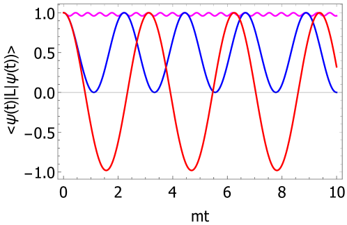
Figure 1: The expectation value of the lepton number is plotted versus $mt$ where $m$ denotes the neutrino mass. The pink colored line shows the relativistic case with $v=0.99$, The blue colored line shows the case with $v=\frac{1}{\sqrt{2}}$. The red colored line shows the non-relativistic case with $v=0.1$.

5 Conclusions

We study the time evolution of lepton number in the Schrödinger picture for a single flavor. Similar to the Heisenberg picture, a multi-flavor Schrödinger is also possible. But the extention to the multi-flavor case is outside of the scope of the paper. The expectation value is the same as that obtained by Heisenberg picture previously. For non-relativistic case, it oscillates with the large amplitude ($\langle\Delta L\rangle\simeq\pm 1$). For relativistic case, it oscillates rapidly with the small amplitude around $\langle L\rangle\simeq 1$. The vacuum with null lepton number is a superposition of the vacuum for mass eigenstate, a pair of Majorana particles, and two pairs of Majorana particles. Similar to the vacuum, the one particle state with the definite lepton number $1$ is a superposition of a mass eigenstate of Majorana neutrino and a state with a Majorana pair and a Majorana neutrino. These non-trivial superposition of states with different energies give rise to the oscillating behavior for the expectation value of lepton number.

Acknowledgement We would like to thank the organizers of the Corfu 2021. The work of T.M. is supported by Japan Society for the Promotion of Science (JSPS) KAKENHI Grant Number JP17K05418.

Appendix A The derivation of Eqs.(13-16) and Eq.(21)

In this appendix, we prove the relations Eqs.(13-16).

$$T(\phi_{p})a^{\dagger}_{M}(\textbf{p},-)T^{-1}(\phi_{p})=\cos\phi_{p}a_{M}^{\dagger}(\textbf{p},-)-i\sin\phi_{p}a_{M}(-\textbf{p},-),$$ (37)

$$T(\phi_{p})a^{\dagger}_{M}(-\textbf{p},-)T^{-1}(\phi_{p})=\cos\phi_{p}a_{M}^{\dagger}(-\textbf{p},-)+i\sin\phi_{p}a_{M}(\textbf{p},-),$$ (38)

with the definition of $T(\phi_{p})$ in Eq.(9) and Eq.(10). One can also compute derivatives,

$$\frac{d^{n}}{d\phi_{p}^{n}}\{T(\phi_{p})a^{\dagger}_{M}(\pm\textbf{p},-)T^{-1}(\phi_{p})\}$$ (39)

$$= i^{n}[g_{p,+}+g_{p,-},[g_{p,+}+g_{p,-},...[g_{p,+}+g_{p,-},\{T(\phi_{p})a^{\dagger}_{M}(\pm\textbf{p},-)T^{-1}(\phi_{p})\}].$$

For $n=2m$($m=$ integer), it is

$$\frac{d^{2m}}{d\phi_{p}^{2m}}\{T(\phi_{p})a^{\dagger}_{M}(\pm\textbf{p},-)T^{-1}(\phi_{p})\}\Bigr{|}_{\phi_{p}=0}=(-1)^{m}a^{\dagger}_{M}(\pm\textbf{p},-).$$ (40)

For $n=2m+1$, it is given by,

$$\frac{d^{2m+1}}{d\phi_{p}^{2m+1}}\{T(\phi_{p})a^{\dagger}_{M}(\pm\textbf{p},-)T^{-1}(\phi_{p})\}\Bigr{|}_{\phi_{p}=0}=(-1)^{m}(\mp i)a_{M}(\mp\textbf{p},-).$$ (41)

They are derived with the following commutation relations,

$$[g_{p,+}+g_{p,-},a^{\dagger}_{M}(\pm\textbf{p},-)]=\mp a_{M}(\mp\textbf{p},-).$$ (42)

Then one can show,

$$T(\phi_{p})a^{\dagger}_{M}(\textbf{p},-)T^{-1}(\phi_{p}) =\left(\sum_{m=0}^{\infty}\frac{(-1)^{m}}{(2m)!}(\phi_{p})^{m}\right)a^{\dagger}_{M}(\textbf{p},-)-i\left(\sum_{m=0}^{\infty}\frac{(-1)^{m}}{(2m+1)!}(\phi_{p})^{m+1}\right)a_{M}(-\textbf{p},-)$$ (43)

$$=\cos\phi_{p}a^{\dagger}_{M}(\textbf{p},-)-i\sin\phi_{p}a_{M}(-\textbf{p},-),$$

$$T(\phi_{p})a^{\dagger}_{M}(-\textbf{p},-)T^{-1}(\phi_{p}) =\cos\phi_{p}a^{\dagger}_{M}(-\textbf{p},-)+i\sin\phi_{p}a_{M}(\textbf{p},-).$$ (44)

This leads to the relations of Eq.(13) and Eq.(14). Eqs.(15-16) can also be proved similarly. Next, the outline of the derivation of Eq.(21) is given as follows;

$$T(\phi_{p})|0_{M}\rangle = \exp[+i\sum_{\lambda=\pm}g_{\lambda}(p)\phi_{p}]|0_{M}\rangle$$

$$= \sum_{n=0}^{\infty}\frac{i^{n}(\phi_{p})^{n}}{n!}(g_{+}(p)+g_{-}(p))^{n}|0_{M}\rangle,$$

where we denote $g_{\lambda}(p)=g_{p,\lambda}$.

$$(g_{+}(p)+g_{-}(p))|0_{M}\rangle = \sum_{\lambda=\pm}B^{\dagger}_{M\lambda}(\textbf{p})|0_{M}\rangle,$$ (45)

$$\{g_{+}(p)+g_{-}(p)\}^{2}|0_{M}\rangle = 2(1+B^{\dagger}_{M-}(\textbf{p})B^{\dagger}_{M+}(\textbf{p}))|0_{M}\rangle,$$ (46)

$$\{g_{+}(p)+g_{-}(p)\}^{3}|0_{M}\rangle = 2\{g_{+}(p)+g_{-}(p)\}(1+B^{\dagger}_{M-}(\textbf{p})B^{\dagger}_{M+}(\textbf{p}))|0_{M}\rangle$$ (47)

$$= 4\{g_{+}(p)+g_{-}(p)\}|0_{M}\rangle$$

$$= 4\sum_{\lambda=\pm}B^{\dagger}_{M\lambda}(\textbf{p})|0_{M}\rangle,$$

$$\{g_{+}(p)+g_{-}(p)\}^{4}|0_{M}\rangle = 4\{g_{+}(p)+g_{-}(p)\}^{2}|0_{M}\rangle.$$ (48)

In deriving Eq.(47), we have used the following anti-commutation relation,

$$\{B_{M\lambda}(\textbf{p}),B^{\dagger}_{M\lambda}(\textbf{p})\} = \alpha_{M}(\textbf{p},\lambda)\alpha^{\dagger}_{M}(\textbf{p},\lambda)+\alpha^{\dagger}_{M}(-\textbf{p},\lambda)\alpha_{M}(-\textbf{p},\lambda)$$ (49)

$$= 1-\alpha^{\dagger}_{M}(\textbf{p},\lambda)\alpha_{M}(\textbf{p},\lambda)+\alpha^{\dagger}_{M}(-\textbf{p},\lambda)\alpha_{M}(-\textbf{p},\lambda).$$

From the consideration above, one concludes that

$$\{g_{+}(p)+g_{-}(p)\}^{2n+1}|0_{M}\rangle=4^{n}\{g_{+}(p)+g_{-}(p)\}|0_{M}\rangle,$$

$$\{g_{+}(p)+g_{-}(p)\}^{2n+2}|0_{M}\rangle=4^{n}\{g_{+}(p)+g_{-}(p)\}^{2}|0_{M}\rangle.$$ (50)

Then one obtains the relation in Eq.(21),

$$T(\phi_{p})|0_{M}\rangle$$ (51)

$$= |0_{M}\rangle+i\sum_{n=0}^{\infty}\frac{(-1)^{n}\phi_{p}^{2n+1}2^{2n}}{(2n+1)!}\{g_{+}(p)+g_{-}(p)\}|0_{M}\rangle+\sum_{n=0}^{\infty}\frac{(-1)^{n+1}\phi_{p}^{2n+2}2^{2n}}{(2n+2)!}\{g_{+}(p)+g_{-}(p)\}^{2}|0_{M}\rangle$$

$$= |0_{M}\rangle-\frac{\sin^{2}\phi_{p}}{2}\{g_{+}(p)+g_{-}(p)\}^{2}|0_{M}\rangle+i\cos\phi_{p}\sin\phi_{p}\{g_{+}(p)+g_{-}(p)\}|0_{M}\rangle$$

$$= \cos^{2}\phi_{p}|0_{M}\rangle+i\cos\phi_{p}\sin\phi_{p}\sum_{\lambda=\pm}B^{\dagger}_{M\lambda}(\textbf{p})|0_{M}\rangle-\sin^{2}\phi_{p}B^{\dagger}_{M-}(\textbf{p})B^{\dagger}_{M+}(\textbf{p})|0_{M}\rangle,$$

where we used the following relations

$$\sum_{n=0}^{\infty}\frac{(-1)^{n}\phi_{p}^{2n+1}2^{2n}}{(2n+1)!}=-\frac{1}{2}\sin^{2}\phi_{p},\quad\sum_{n=0}^{\infty}\frac{(-1)^{n+1}\phi_{p}^{2n+2}2^{2n}}{(2n+2)!}=\cos\phi_{p}\sin\phi_{p}.$$ (52)

Appendix B The derivation of Eq.(25)

In this appendix, we derive the relation which is used to derive Eq.(25),

$$\sqrt{\cos 2\phi_{q}}(\cos\phi_{q}a^{\dagger}_{M}(\textbf{q},-)-i\sin\phi_{q}a_{M}(-\textbf{q},-))$$ (53)

$$\times\{\cos^{2}\phi_{q}-\sin^{2}\phi_{q}B^{\dagger}_{M+}(\textbf{q})B^{\dagger}_{M-}(\textbf{q})+i\sin\phi_{q}\cos\phi_{q}\sum_{\lambda=\pm}B^{\dagger}_{M\lambda}(\textbf{q})\}|0_{M}\rangle$$

$$= \sqrt{\cos 2\phi_{q}}\{(\cos^{3}\phi_{q}+\sin^{2}\phi_{q}\cos\phi_{q})a_{M}^{\dagger}(\textbf{q},-)$$

$$+i(\sin\phi_{q}\cos^{2}\phi_{q}+\sin^{3}\phi_{q})B^{\dagger}_{M+}(\textbf{q})a_{M}^{\dagger}(\textbf{q},-)\}|0_{M}\rangle$$

$$= \sqrt{\cos 2\phi_{q}}\{\cos\phi_{q}a_{M}^{\dagger}(\textbf{q},-)+i\sin\phi_{q}B^{\dagger}_{M+}(\textbf{q})a_{M}^{\dagger}(\textbf{q},-)\}|0_{M}\rangle.$$

References

- [1] A. S. Adam, N. J. Benoit, Y. Kawamura, Y. Matsuo, T. Morozumi, Y. Shimizu, Y. Tokunaga and N. Toyota, PTEP doi.org/10.1093/ptep/ptab025, arXiv:2101.07751.
- [2] N. N. Bogolyubov, Nuovo Cim. 7, 794-805 (1958) doi:10.1007/BF02745585.
- [3] M. Blasone and G. Vitiello, Annals Phys. 244, 283-311 (1995) [erratum: Annals Phys. 249, 363-364 (1996)] doi:10.1006/aphy.1995.1115 [arXiv:hep-ph/9501263 [hep-ph]].
- [4] A. Tureanu, Phys. Rev. D 98, no.1, 015019 (2018) doi:10.1103/PhysRevD.98.015019 [arXiv:1804.06433 [hep-ph]].
- [5] K. Fujikawa, Phys. Lett. B 781, 295-301 (2018) doi:10.1016/j.physletb.2018.04.004 [arXiv:1801.06960 [hep-th]].
- [6] A. S. Adam, N. J. Benoit, Y. Kawamura, Y. Mastuo, T. Morozumi, Y. Shimizu, Y. Tokunaga and N. Toyota, doi:10.31526/ACP.BSM-2021.29 [arXiv:2105.04306 [hep-ph]].