Long-tailed Extreme Multi-label Text Classification
with Generated Pseudo Label Descriptions

Abstract

Extreme Multi-label Text Classification (XMTC) has been a tough challenge in machine learning research and applications due to the sheer sizes of the label spaces and the severe data scarce problem associated with the long tail of rare labels in highly skewed distributions. This paper addresses the challenge of tail label prediction by proposing a novel approach, which combines the effectiveness of a trained bag-of-words (BoW) classifier in generating informative label descriptions under severe data scarce conditions, and the power of neural embedding based retrieval models in mapping input documents (as queries) to relevant label descriptions. The proposed approach achieves state-of-the-art performance on XMTC benchmark datasets and significantly outperforms the best methods so far in the tail label prediction. We also provide a theoretical analysis for relating the BoW and neural models w.r.t. performance lower bound.

1 Introduction

Extreme multi-label text classification (XMTC) is the task of tagging documents with relevant labels in a very large and often skewed candidate space. It has a wide range of applications, such as assigning subject topics to news or Wikipedia articles, tagging keywords for online shopping items, classifying industrial products for tax purposes, and so on.

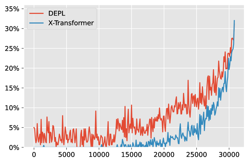
Figure 1: The classification performance of X-Transformer and DEPL (ours) on the Wiki10-31K dataset. The curves show the macro-averaged $F1@19$ scores of each system over the label bins (with 100 labels per bin).

The most difficult part in solving the XMTC problem is to train classification models effectively for the rare labels in the long tail of highly skewed distributions, which suffers severely from the lack of sufficient training instances. Efforts addressing this challenge by the text classification community include hierarchical regularization methods for large margin classifiers Gopal and Yang (2013), Bayesian modeling of graphical or hierarchical dependencies among labels Gopal and Yang (2010); Gopal et al. (2012), clustering-based divide-and-conquer strategies in resent neural classifiers Chang et al. (2020); Khandagale et al. (2019); Prabhu et al. (2018), and so on. Despite the remarkable progresses made so far, and the problem is still very far from being well solved. Figure 1 shows the performance of X-Transformer Chang et al. (2020), one of the state-of-the-art (SOTA) XMTC models with the best published result so far on the Wiki10-31k benchmark dataset (with over 30,000 unique labels). The horizontal axis in this figure is the ranks of the labels sorted from rare to common, and the vertical axis is the text classification performance measured in macro-averaged $F1@19$ (higher the better) for binned labels (100 labels per bin). The blue curve is the result of X-Transformer, which has the scores close to $0$ (worst possible score) for nearly half of the total labels. In other words, SOTA methods in XMTC still perform poorly in tail label prediction. We should point out that such poor performance of XMTC classifiers on tail labels has been largely overlooked in the recent literature, because benchmark evaluations of SOTA methods have typically used the metrics that are dominated by the system’s performance on common labels, such as the micro-averaged precision at top-k (P@k). As a proper choice for evaluation of tail label prediction in figure 1, macro-averaged $F1@k$ is used, which gives the performance on each label an equal weight in the average. The red curve in the figure is the result of our new approach, being introduced the next.

In this paper, we seek solutions for tail label prediction from a new angle: we introduce a novel framework, namely the Dual Encoder with Pseudo Label (DEPL). It treats each input document as a query and uses a neural network model to retrieve relevant labels from the candidate space based on the textual descriptions of the labels. The underlying assumption is, if the label descriptions are highly informative for text-based matching, then the retrieval system should be able to find relevant labels for input documents. Such a system would be particularly helpful for tail label prediction as the retrieval effectiveness does not necessarily rely on the availability of a large number of training instances, which what the tail labels are lacking.

Now the key question is, how can we get a highly informative description for each label without human annotation? In reality, class names are often available but they are typically one or two words, which cannot be sufficient for retrieval-based label prediction. Our answer is to use a relatively simple trained classifier, e.g., a linear support vector machine (SVM), to automatically generate an informative description for each label, which we call the pseudo description of the label. The reason for us to choose a traditional classifier like linear SVM instead of a more modern neural model for label descriptions generation is that we want to better leverage the unsupervised statistics about word usage such as TF (term frequency within a document) and IDF (the inverse document frequencies within a document collection). Such unsupervised word features would be particularly helpful to alleviate the difficulty in classifier training under extreme data scarce conditions, and are easy and natural for traditional classifiers like SVM to leverage. The result of our approach (DEPL) is shown as the red curve in Figure 1, which significantly outperforms the blue curve of X-Transformer not only in the tail-label region but also in all other regions. We also observed similar improvements by DEPL over strong baselines on other benchmark datasets (see section 6).

Our main contributions can be summarized as the following:

1. We formulate the XMTC task as a neural retrieval problem, which enables us to alleviate the difficulty in tail label prediction by matching documents against label descriptions with advanced neural retrieval techniques.

2. We enhance the retrieval system with pseudo label descriptions generated by a BoW classifier, which is proven to be highly effective for improving tail label prediction under severe data scarce conditions.

3. Our proposed method significantly and consistently outperforms strong baselines on multiple challenging benchmark datasets. Ablation tests provide in-depth analysis on different settings in our framework. A theoretical analysis for relating the BoW and neural models w.r.t. performance lower bound is also provided.

2 Related Work

BoW (or Sparse) Classifier

Traditional BoW classifiers rely on the bag-of-words features such as one-hot vector with tf-idf weights, which capture the word importance in a document. Since the feature is high dimenstional and sparse, we call the BoW classifiers the sparse classifiers. Early examples include the one-vs-all SVM models such as DiSMEC Babbar and Schölkopf (2017), ProXML Babbar and Schölkopf (2019) and PPDSparse Yen et al. (2017). Later methods leverage the tree structure of the label space for more effective or scalable learning, such as Parabel Prabhu et al. (2018) and Bonsai Khandagale et al. (2019). Since tf-idf features rely on surface-level word matching, sparse classifiers tend to miss the semantic matching among lexical variants or related concepts in different wording.

Neural (or Dense) Classifier

Neural models learn to capture the high level semantics of documents with dense feature embeddings. For this reason, we call them the dense classifiers. The XML-CNN Liu et al. (2017) and SLICE Jain et al. (2019) employ the convolutional neural network on word embeddings for document representation. More recently, X-Transformer Chang et al. (2020), LightXML Jiang et al. (2021) and APLC-XLNet Ye et al. (2020) tames large pre-trained Transformer models to encode the input document into a fixed vector. AttentionXML You et al. (2018) applies a label-word attention mechanism to calculate label-aware document embeddings, but it requires more computational cost proportional to the document length. In the above neural models, the feature extractor and the label embedding (randomly initialized) are jointly optimized via supervised signals. As we will show later, the document and the label embedding can be insufficiently optimized for the tail labels whose supervision signals are mostly negative.

Hybrid Approach:

X-Transformer (Chang et al., 2020) complements neural model with sparse feature by concatenating tf-idf with the learned cluster-level neural embedding, which is an ensemble of the sparse and dense classifiers. Recent works in retrieval design unified systems to combine the sparse and dense features for better performance. SPARC Lee et al. (2019) learns contextualized sparse feature indirectly via Transformer attention. COIL Gao et al. (2021) leverages lexical matching of contextualized BERT embeddings, and CLEAR Gao et al. (2004) designs a residual-based loss function for the neural model to learn hard examples from a sparse retrieval model. While we also combine the sparse feature with neural model, the classification setting does not assume predefined label description as in the retrieval setting.

Label Description:

When both the document text and label descriptions are available, the ranked-based multi-label classification is similar to the retrieval setting, where the dual encoder models Gao and Callan (2021); Xiong et al. (2020); Luan et al. (2020); Karpukhin et al. (2020) have achieved SOTA performance in information retrieval on large benchmark datasets with millions of passages. The Siamese network Dahiya et al. (2021) for classification encodes both input documents and label descriptions under the assumption that high quality label descriptions are available. Chai et al. (2020) tries a generative model with reinforcement learning to produce extended label description with predefined label descriptions for initialization and uses cross attentions between input text document and output labels. Although their ideas of utilizing label descriptions are attractive, the performance of those systems crucially depends on availability of predefined high-quality label descriptions, which is often difficult to obtain in real-world applications. Instead, the realistic label descriptions are often short, noisy and insufficient for lexicon-matching based label prediction for input documents. How to generate informative label descriptions without human efforts is thus an important problem, for which we offer an algorithmic solution in this paper.

Figure 2: The proposed DEPL framework. First, we train a BoW classifier (SVM) and extract the top keywords from the label embeddings according to the learned token importance. Then, we concatenate the keywords with the original label names to form pseudo descriptions. Finally, we leverage the neural retrieval model to rank the labels according to semantic matching between document text and label descriptions.

3 Proposed Method

In this section,we first provide the preliminaries on multi-label text classification system. Then we discuss the generation of pseudo label description obtained from a sparse classifier, the design of DEPL from the retrieval perspective, and the enhanced classification system with the retrieval module.

3.1 Preliminaries

Let $\mathcal{D}=\{\left(\mathbf{x}_{i},\mathbf{y}_{i}\right)_{i=1}^{N_{\text{train}}}\}$ be the training data where $\mathbf{x}_{i}$ is the input text and $\mathbf{y}_{i}\in\{0,1\}^{L}$ are the binary ground truth labels of size $L$. Given an instance ${\bm{x}}$ and a label $l$, a classification system produces a matching score of the text and label:

$$f({\bm{x}},l)=\langle\phi({\bm{x}}),{\bm{w}}_{l}\rangle$$

where $\phi({\bm{x}})$ represent the document feature vector and ${\bm{w}}_{l}$ represents the label embedding of $l$. The dot product $\langle\cdot,\cdot\rangle$ is used as the similarity function.

Typically, the label embedding ${\bm{w}}_{l}$ is randomly initialized and trained from the supervised signal. While learning the embedding as free parameters is expressive when data is abundant, it could be difficult to be optimized under the data scarce situation.

Sketch of Method

To tackle the long-tailed XMTC problem, we propose DEPL, a neural retrieval framework with generated pseudo label descriptions, as shown in figure 2. Instead of learning the label embedding from scratch, the retrieval module directly leverages the semantic matching between the document and label text, providing a strong inductive bias on tail label prediction.

Furthermore, we will show in later sections that a BoW classifier with the statistical feature gives better performance in data scarce situation. The pseudo labels generated from a BoW classifier exploit such data heuristics, and the neural model complements the statistical information with semantic meaning for further improvement. Next, we introduce the components of our system in details.

3.2 Pseudo Label Description

Short label names are usually given in the benchmark dataset, such as the category name of an Amazon product or the could tag of a Wikipedia article. However, the provided label name is usually noisy and ambiguous, of which the precise meaning need to be inferred from the document text (refer to section 6 for more detailed discussions). Therefore, we enhance the quality of label names by an augmentation with keywords generated from a sparse classifier. While there are multiple choices of the sparse classifier, we pick the linear SVM model with tf-idf feature $\phi_{t}({\bm{x}})$ for a balance between efficiency and performance:

$$f_{\text{sparse}}({\bm{x}},l)=\langle\phi_{t}({\bm{x}}),{\bm{w}}^{\text{svm}}_{l}\rangle$$

The label embedding weight ${\bm{w}}^{\text{svm}}_{l}$ is optimized with the hinge loss:

$$\mathcal{L}_{\text{hinge}}=\frac{1}{LB}\sum_{i=1}^{B}\sum_{l=1}^{L}\max(0,1-\tilde{y}_{l}\cdot f_{\text{sparse}}({\bm{x}}_{i},l))$$

where $\tilde{y}_{l}=2y_{l}-1\in\{-1,1\}$ and $B$ is the batch size.

For a train SVM model, ${\bm{w}}^{\text{svm}}_{l}$ has the dimension equal to the vocabulary size and each value ${w}^{\text{svm}}_{li}$ of the label embedding denotes the importance of the token $i$ w.r.t label $l$. We select the top $k$ most important tokens (ranked according to the importance score) as keywords, which are appended to the original label name to form the pseudo label description:

$$\operatorname{pseudo\_label}(l)=\operatorname{label\_name}(l)\oplus\operatorname{keywords}(l)$$

where $\oplus$ is the append operation. The token importance learned in ${\bm{w}}^{\text{svm}}_{l}$ is purely based on the statistics of word frequency. After we extract the tokens as keywords, we can additionally leverage the semantic meaning of them with the powerful neural network representations, which will be introduced in the next section.

3.3 Retrieval Model with Label Text

In the long-tailed XMTC problem, the training instances of document and label pair for tail labels are limited, and thus it is difficult to optimize for neural model with a large number of parameters. Instead, we use a dual encoder model Gao and Callan (2021); Xiong et al. (2020); Luan et al. (2020); Karpukhin et al. (2020) to leverage the semantic matching of document and label text. We use the BERT Devlin et al. (2018) model as our design choice as the contextualized function, which is shared for both the document and label text encoding. The similarity between them is measured by the dot product:

$$f_{\text{dual}}({\bm{x}},l)=\langle\phi_{\text{doc}}({\bm{x}}),\phi_{\text{label}}(\operatorname{text}(l))\rangle$$

where $\operatorname{text}(l)$ is the textual information of the label $l$. When the textual information only includes the label name given in the dataset, we call the model DE-ret. Otherwise, when the textual information is the pseudo label, we call the model DEPL.

The document embedding $\phi_{\text{doc}}({\bm{x}})$ is obtained from the CLS embedding of the BERT model followed by a linear pooling layer:

$$\phi_{\text{doc}}({\bm{x}})={\bm{W}}_{doc}\cdot\operatorname{BERT}({\bm{x}},\text{CLS})+{\bm{b}}_{doc}$$

where $\operatorname{BERT}(\operatorname{text}(l),\text{CLS})$ represents the contextualized embedding of the special CLS token. ${\bm{W}}_{doc}$ and ${\bm{b}}_{doc}$ are the weights and biases for the document pooler layer.

For the label embedding $\phi_{\text{label}}(\operatorname{text}(l))$, we take an average of the last hidden layer of BERT followed by a linear pooler layer:

$$\phi_{\text{label}}(\operatorname{text}(l))={\bm{W}}_{label}\cdot\psi_{bert}(\operatorname{text}(l))+{\bm{b}}_{label}$$ (1)

$$\psi_{bert}(\operatorname{text}(l))=\frac{1}{|\operatorname{text}(l)|}\sum_{j=1}^{|\operatorname{text}(l)|}\operatorname{BERT}(\operatorname{text}(l),j)$$ (2)

where $\operatorname{BERT}(\operatorname{text}(l),j)$ represents the contextualized embedding of the $j$-th token in $\operatorname{text}(l)$ obtained from the last hidden layer of the BERT model. ${\bm{W}}_{label}$ and ${\bm{b}}_{label}$ are the weights and biases for the label pooler layer. In the equation 2, the average embedding of label tokens yields better performance empirically than the CLS embedding for two potential reasons: 1) the keywords ranked by importance are not natural language and the CLS embedding may not effectively aggregate such type of information, and 2) the CLS embedding captures the global semantic of longer context while the average of token preserves more of the shorter label text meaning.

Learning with Negative Sampling

In order to optimize $f_{\text{dual}}({\bm{x}},l)$, we need to calculate the label embedding $\phi_{\text{label}}(\operatorname{text}(l))$. Since calculating all the label embeddings for each batch is both expensive and prohibitive by the memory limit, we resort to negative sampling strategies for in-batch optimization. Specifically, we sample a fix-sized subset of labels for each batch containing: 1) all the positive labels of the instances in the batch, 2) the top negative predictions by the sparse classifier as the hard negatives, and 3) the rest of the batch is filled with uniformly random sampled negatives labels.

Let ${\mathbb{S}}_{b}$ be the subset of labels sampled for a batch. The objective for the dual encoder is:

$$\begin{split}\mathcal{L}_{\text{dual}}=-\frac{1}{B|{\mathbb{S}}_{b}|}\sum_{i=1}^{B}\Bigg{(}\Bigg{.}\sum_{p\in{\bm{y}}_{i}^{+}}\log\sigma(f_{\text{dual}}({\bm{x}}_{i},p))\\ +\sum_{n\in{\mathbb{S}}_{b}\backslash{\bm{y}}_{i}^{+}}\log\sigma((1-f_{\text{dual}}({\bm{x}}_{i},n)))\Bigg{.}\Bigg{)}\end{split}$$

where $B$ is the batch size, ${\bm{y}}_{i}^{+}$ is the postive labels for instance $i$, and $\sigma$ is the sigmoid function.

3.4 Enhance Classification with Retrieval

In the neural classification system, the label embedding is treated as free parameters to be learned from supervised data, which is more expressive for medium and head labels with abundant training instances. The dense classifier learns the function:

$$f_{\text{dense}}({\bm{x}},l)=\langle\phi_{\text{doc}}({\bm{x}}),{\bm{w}}_{l}^{\text{neural}}\rangle$$ (3)

We propose to enhance the classification model with the retrieval mechanism by jointly fine-tuning:

$$f_{\text{cls-dual}}({\bm{x}},l)=\frac{\sigma(f_{\text{dual}}({\bm{x}},l))+\sigma(f_{\text{dense}}({\bm{x}},l))}{2}$$ (4)

The classification and retrieval modules share the same BERT encoder. We refer to the system as DEPL+c. The object function $\mathcal{L}_{\text{cls-dual}}$ is similar to $\mathcal{L}_{\text{dual}}$ except for replacing $f_{\text{dual}}$ with $f_{\text{\text{cls-dual}}}$.

The DEPL+c model looks like an ensemble of the two systems at the first sight, but there are two major differences: 1) As the BERT encoder is shared between the classification and retrieval modules, it doesn’t significantly increase the number of parameters as in Chang et al. (2020); Jiang et al. (2021); and 2) when the two modules are optimized together, the system can take advantages of both units according to the situation of head or tail label predictions.

4 Theoretical Analyses of DEPL

In this section, we first discuss the relation between dense and sparse classifier and then we derive a lower bound performance of DEPL over the sparse classifier.

4.1 Rethinking Dense and Sparse XMTC

We analyze the document and label embedding optimization in the skewed label distribution from the gradient perspective. Specifically, recall the predicted probability optimized by the binary cross entropy (BCE) loss:

$$\mathcal{L}_{\text{BCE}}=-\sum_{l=1}^{L}y_{l}\log p_{l}+(1-y_{l})\log(1-p_{l})$$

The derivative of $\mathcal{L}_{\text{BCE}}$ w.r.t the logits is:

$$\frac{\partial\mathcal{L}_{\text{BCE}}}{\partial s_{l}}=\begin{cases}p_{l}-1&\text{if }y_{l}=1\\ p_{l}&\text{otherwise}\\ \end{cases}$$

Document Feature Learning

In multi-label classification, the document feature needs to reflect all the representations of relevant labels. In fact, the gradient describes the relation between feature $\phi_{n}({\bm{x}})$ and label embedding ${\bm{w}}_{l}$. By the chain rule, the gradient of $\mathcal{L}_{\text{BCE}}$ w.r.t the document feature is:

$$\frac{\partial\mathcal{L}_{\text{BCE}}(y_{l},p_{l})}{\partial\phi_{n}({\bm{x}})}=\begin{cases}(p_{l}-1){\bm{w}}_{l}&\text{if }y_{l}=1\\ p_{l}{\bm{w}}_{l}&\text{otherwise}\\ \end{cases}$$

By optimizing parameters $\theta$ of feature extractor, the document representation is encourage to move away from the negative label representation, that is:

$$\phi_{n}({\bm{x}};\theta^{\prime})\leftarrow\phi_{n}({\bm{x}};\theta)-\eta p_{l}{\bm{w}}_{l}$$

where $\eta$ is the learning rate. Since a tail label appears more often as negative labels and $\theta$ is shared for all the data, the feature extractor is unlikely to encode tail label information, making tail labels more difficult to be predicted. In comparison, the sparse feature like tf-idf is unsupervised from corpus statics, which does not suffer from this problem. The feature may still maintain the representation power to separate the tail labels.

Label Feature Learning

When the labels are treated as indices in a classification system, they are randomly initialized and learned from supervised signals. The gradients of $\mathcal{L}_{\text{BCE}}$ w.r.t the label feature is:

$$\frac{\partial\mathcal{L}_{\text{BCE}}(y_{l},p_{l})}{\partial{\bm{w}}_{l}}=\begin{cases}(p_{l}-1)\phi_{n}({\bm{x}})&\text{if }y_{l}=1\\ p_{l}\phi_{n}({\bm{x}})&\text{otherwise}\\ \end{cases}$$

The label embedding is updated by:

$${\bm{w}}_{l}^{\prime} ={\bm{w}}_{l}+\frac{\eta}{N_{\text{train}}}\sum_{i:y_{il}=1}(1-p_{il})\phi_{n}({\bm{x}}_{i})$$

$$-\frac{\eta}{N_{\text{train}}}\sum_{i:y_{il}=0}p_{il}\phi_{n}({\bm{x}}_{i})$$

As most of the instances are negative for a tail label, the update of tail label embedding is inundated with the aggregation of negative features, making it hard to encode distinctive feature reflecting its identity. Therefore, learning the tail label embedding from supervised signals alone can be very distracting. Although previous works leverage negative sampling to alleviate the problem Jiang et al. (2021); Chang et al. (2020), we argue that it is important to initialize the label embedding with the label side information.

4.2 Analysis on Performance Lower Bound

We will show that DEPL achieves a lower bound performance as the sparse classifier, given the selected keywords are important and the sparse classifier can separate the positive from the negative instances with non-trivial margin.

Let $\phi_{t}({\bm{x}})$ be the normalized tf-idf feature vector of text with $\|\phi_{t}({\bm{x}})\|_{2}=1$. The sparse label embeddings $\{{\bm{w}}_{1},\ldots,{\bm{w}}_{L}\}$ satisfies $\|{\bm{w}}_{l}\|_{2}\leq 1,w_{li}>0$. In fact, label embeddings can be transformed to satisfy the condition without affecting the prediction rank. Let ${\bm{z}}_{l}$ be the top selected keywords from the sparse classifier, which is treated as the pseudo label. Define the sparse keyword embedding ${\bm{v}}_{l}$ with ${v}_{li}={w}_{li}$ if $i$ is an index of selected keywords and $0$ otherwise.

In the following, we define the keyword importance and the classification error margin.

Definition 1.

For label $l$ and $\delta\geq 0$, the sparse keyword embedding ${\bm{v}}_{l}$ is $\delta$-bounded if $\langle\phi_{t}({\bm{x}}),{\bm{v}}_{l}\rangle\geq\langle\phi_{t}({\bm{x}}),{\bm{w}}_{l}\rangle-\delta$.

Definition 2.

For two labels $p$ and $n$, the error margin $\mu$ is the difference between the predicted scores $\mu(\phi({\bm{x}}),{\bm{w}}_{p},{\bm{w}}_{n})=\langle\phi({\bm{x}}),{\bm{w}}_{p}-{\bm{w}}_{n}\rangle$.

We state the main theorem below:

Theorem 3.

Let $\phi_{t}({\bm{x}})$ and $\phi_{n}({\bm{x}})$ be the sparse and dense (dimension $d$) document feature, ${\bm{w}}_{l}$ be the label embedding and ${\bm{z}}_{l}$ be the $\delta$-bounded keywords. For a positive label $p$, let ${\mathbb{N}}_{p}=\{n_{1},\ldots,n_{M_{p}}\}$ be a set of negative labels ranked lower than $p$. The error margin $\epsilon_{i}=\mu(\phi_{t}({\bm{x}}),{\bm{w}}_{p},{\bm{w}}_{n_{i}})$ and $\epsilon=\min(\{\epsilon_{1},\ldots,\epsilon_{M_{p}}\})$. An error ${\mathcal{E}}_{i}$ of the neural classifier occurs when

$$\mu(\phi_{n}({\bm{x}}),\phi_{n}({\bm{z}}_{p}),\phi_{n}({\bm{z}}_{n_{i}}))\leq 0$$ (5)

The probability of any such error happening satisfies

$$P({\mathcal{E}}_{1}\cup\ldots\cup{\mathcal{E}}_{M_{p}})\leq 4{M_{p}}\exp(-\frac{(\epsilon-\delta)^{2}d}{50})$$

When $(\epsilon-\delta)\geq 10\sqrt{\frac{\log M_{p}}{d}}$, the probability is bounded by $\frac{1}{M_{p}}$.

Discussion: An error event occurs when the sparse model makes a correct prediction but the neural model doesn’t. If the neural model avoids all such errors, the performance should be at least as good as the sparse model, and Theorem 3 gives a bound of that probability.

The term $\delta$ measures the importance of selected keywords (smaller the more important), the error margin $\epsilon$ measures the difficulty the correctly predicted positive and negative pairs by the sparse model. The theorem states that the model achieves a lower bound performance as sparse classifier if the keywords are informative and error margin is non-trivial. Proofs and assumptions are in section A for interested readers.

5 Evaluation Design

5.1 Datasets

The benchmark datasets for our experiments are EURLex-4K (Loza Mencía and Fürnkranz, 2008), Wiki10-31K (Zubiaga, 2012) and AmazonCat-13K (McAuley and Leskovec, 2013). The Wiki10-31K and AmazonCat-13K were obtained from the Extreme Classification Repository. As for EURLex-4K, we obtained an unstemmed version from the APLC-XLNet github. Table 1 summarizes the corpus statistics.

Table 1: Corpus Statistics: $N_{\text{train}}$ and $N_{\text{test}}$ are the number of training and testing instances respectively; $\bar{L}_{d}$ is the average number of labels per document, and $L$ is the number of unique labels in total; $|{\mathbb{L}}_{\text{tail}}|$ is the number of tail labels with $1\sim 9$ positive training instances.

Dataset $N_{train}$ $N_{test}$ $\bar{L}_{d}$ $L$ $|{\mathbb{L}}_{\text{tail}}|$ EURLex-4K 15,539 3,809 5.30 3,956 2,413 Wiki10-31K 14,146 6,616 18.64 30,938 26,545 AmazonCat-13K 1,186,239 306,782 5.04 13,330 3,936

For comparative evaluation of methods in tail label prediction, from each of the three corpora we extracted the subset of labels with $1\sim 9$ positive training instances. Those tail-label subsets include $63.48\%$, $88.65\%$ and $29.53\%$ of the total labels in the three corpora, respectively. These numbers indicate that the label distributions are indeed highly skewed, with a heavy long tail in each corpus.

5.2 Evaluation Metrics

We use three metrics which are commonly used in XMTC evaluations, namely, the micro-averaged $P@k)$, the PSP@k Jain et al. (2016a); Wei et al. (2021), and the macro-averaged $F1@k$.

Given a ranked list of the predicted labels for each test document, the precision of the top-k labels is defined as:

$$P@k=\frac{1}{k}\sum_{i=1}^{k}\mathbbm{1}_{{\bm{y}}_{i}^{+}}(p_{i})$$ (6)

where $p_{i}$ is the $i$-th label in the list ${\bm{p}}$ and $\mathbbm{1}_{{\bm{y}}_{i}^{+}}$ is the indicator function. The average of the $P@k$ values across all the test-set documents is called micro-averaged P@k, which has been the most commonly used in XMTC evaluations. Since this metric gives an equal weight to the per-instance scores, the resulted average is dominated by the system’s performance on the common (head) labels but not the tail labels. In other words, the performance comparison in this metric cannot provide enough insights to the effectiveness of methods in tail label prediction.

As an alternative metric, PSP@k  Jain et al. (2016a) re-weights the precision on each instance as:

$$PSP@k=\frac{1}{k}\sum_{l=1}^{k}\frac{\mathbbm{1}_{\mathbf{y}}(\mathbf{p}_{l})}{\operatorname{prop}(\mathbf{p}_{l})}$$

where the propensity score $\operatorname{prop}(\mathbf{p}_{l})$ in the denominator gives higher weights to tail labels.

Macro-averaged F1@k Yang and Liu (1999) is a metric that gives an equal weight to all the labels, including tail labels, head labels and any labels in the middle range. It is defined as the average of the label-specific $F1@k$ values, calculated based on a contingency table for each label, as shown in table 2. Specifically, the precision, recall and $F1$ for a predicted ranked list of length $k$ are computed as $\mathrm{P}=\frac{\mathrm{TP}}{\mathrm{TP}+\mathrm{FP}},\mathrm{R}=\frac{\mathrm{TP}}{\mathrm{TP}+\mathrm{FN}}$, and $\operatorname{F1}=2\frac{P\cdot R}{P+R}$.

Table 2: Contingency table for label $l$.

$l$ is true label $l$ is not true label $l$ is predicted True Positive ($\mathrm{TP}_{l}$) False Positive ($\mathrm{FP}_{l}$) $l$ is not predicted False Negative ($\mathrm{FN}_{l}$) True Negative ($\mathrm{TN}_{l}$)

For micro-averaged P@k and PSP@k, we choose $k=1,3,5$ as in previous works. For macro-averaged F1@k, we choose $k=19$ for Wiki10-31K because it has an average of $18.64$ labels and $k=5$ for the rest datasets.

5.3 Baselines

For the tail label evaluation, our method is compared with the SOTA deep learning models including X-Transformer Chang et al. (2020), XLNet-APLC Ye et al. (2020), LightXML Jiang et al. (2021), and AttentionXML You et al. (2018). X-Transformer, LightXML, and XLNet-APLC employ pre-trained Transformers for document representation. We reproduced the results of single model (given in their implementation) predictions with BERT as the base model for LightXML, BERT-large for X-Transformer, XLNet for XLNet-APLC, and LSTM for AttentionXML. The AttentionXML utilizes label-word attention to generate label-aware document embeddings, while the other models generate fixed document embedding.

For the overall prediction of all labels, we also include the baselines of sparse classifiers: DisMEC Babbar and Schölkopf (2017), PfastreXML Jain et al. (2016b), Parabel Prabhu et al. (2018), Bonsai Khandagale et al. (2019), and we use the published results for comparison. We provide an implementation of linear SVM model with our extracted tf-idf features as another sparse baseline, and a BERT-base classifier as another dense classifier (used to initialize DEPL).

5.4 Implementation Details

For the sparse model, since the public available BoW feature doesn’t have a vocabulary dictionary, we generate the tf-idf feature by ourselves. We tokenize and lemmatize the raw text with the Spacy Honnibal and Montani (2017) library and extract the tf-idf feature with the Sklearn Pedregosa et al. (2011) library, with unigram whose df is $>=2$ and $<=70\%$ of the total documents. We use the BERT model as the contextualize function for our retrieval model, which is initialized with a pretrained dense classifier. Specifically, we fine-tune a $12$ layer BERT-base model with different learning rates for the BERT encoder, BERT pooler and the classifier. The learning rates are $(1e-5$, $1e-4$, $1e-3)$ for Wiki10-31K and $(5e-5$, $1e-4$, $2e-3)$ for the rest datasets. For the negative sampling, we sample batch of 500 instances for Wiki10-31K, and $300$ for EURLex-4K and AmazonCat-13K. We include $10$ hard negatives predicted by the SVM model for each instances. We used learning rate $1e-5$ for fine-tuning the BERT of our retrieval model and $1e-4$ for the pooler and label embeddings. For the pseudo label descriptions, we concatenate the provided label description with the generated the top $20$ keywords. The final length is truncated up to $32$ after BERT tokenization. We use length $16$ of pseudo label description as the default setting for DEPL.

Table 3: Tail label prediction results of methods in $P@k$ on the labels with $1\sim 9$ positive training instances.

EURLex-4K Wiki10-31K AmazonCat-13K Methods PSP@1 PSP@3 PSP@5 PSP@1 PSP@3 PSP@5 PSP@1 PSP@3 PSP@5 X-Transformer 37.85 47.05 51.81 13.52 14.62 15.63 51.42 66.14 75.57 XLNet-APLC 42.21 49.83 52.88 14.43 15.38 16.47 52.55 65.11 71.36 LightXML 40.54 47.56 50.50 14.09 14.87 15.52 50.70 63.14 70.13 AttentionXML 44.20 50.85 53.87 14.49 15.65 16.54 53.94 68.48 76.43 SVM 39.18 48.31 53.37 11.84 14.00 15.81 51.83 65.41 72.82 DEPL 45.60 52.28 53.52 16.30 16.26 16.27 55.94 70.01 76.87 DEPL+c 44.60 52.74 54.64 14.90 15.53 16.20 55.21 69.73 75.94

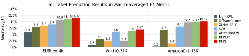
Figure 3: Tail-label prediction results in $F1@k$ on the labels with $1\sim 9$ positive training instances, with $k=5$ for the EURLex-4K and AmazonCat-13K datasets, and $k=19$ for the Wiki10-31K dataset.

6 Results

Our experiments investigate the effectiveness of our model on the tail label prediction as well as its performance on the overall prediction.

6.1 Results in Tail Label Prediction

PSP Metric

The evaluation with the PSP metric is shown in table 3. We compare our model with the SOTA deep learning methods. Our proposed models DEPL and DEPL+c perform the best on the three benchmark datasets.

Since the Wiki10-31K dataset has more labels and the distribution is more skewed, the observation on the results is very interesting. On the one hand, the most frequent label covers more than $85\%$ of the training instances, so it is easier to predict that label than other lower frequencies labels. However, ranking the high frequency labels at the top doesn’t give much gain on the PSP metric. On the other hand, each instance has an average of $19$ positive labels and ranking the subset of tail labels at the top could boost the PSP score. Since DEPL relies on the semantic matching between the document and label text, it is less affected by the dominating training pairs, and thus the PSP@1, PSP@3 beats the SOTA models by a larger margin. The DEPL+c achieves worse performance on this dataset, because the classification counterpart of the model would benefit more on the head label predictions and tend to rank the head labels at the top.

For the EURLex-4K and AmazonCat-13K, we don’t observe to much difference in DEPL and DEPL +c performance, and even DEPL +c can perform better on the EURLex-4K dataset. This maybe due to the improvement of head label predictions which can also boost the overall score in the micro-based metric.

Macro-F1 Metric

Although the PSP metric gives higher weight to the tail labels, it is a micro-averaged metric over the scores of each instance, which can still be affected by the high frequency labels that cover most of the instances. In comparison, the Macro-averaged F1 metric gives each label an equal weight and reflects more of the label level performance. We compare the Macro F1 metric averaged on the tail labels and the results are shown in figure 3.

An interesting observation is that the SVM baseline achieves competitive results on the tail label predictions. We observe that SVM model can outperform all the pre-trained Transformer-based models on the tail label prediction, and outperform the AttentionXML on the Wiki10-31K dataset. We guess the reason is that the SVM utilizes the unsupervised statistical feature as document representation, which potentially suffers less from the data scarcity issue. The empirical result also serves as an evidence that the joint optimization of feature extractor and label embedding is difficult when data is limited. Among the deep learning baselines, the AttentionXML method performs the best on the tail label predictions, beating the SVM on $2$ out of the $3$ benchmark datasets. The reason could be that it utilizes the label to document word attention which is a local feature matching that benefits the tail label prediction.

Our proposed models perform the best on the Macro F1 metric with the DEPL model showing the best performance on all the $3$ benchmark datasets. We attribute the success of model to the retrieval module that focuses on the semantic matching between the document and label text. While the results evaluated in the Macro-averaged F1 metric show similar trend to that in the PSP metric, we do get some different conclusions with different metrics, i.e. the SVM model doesn’t stand out under the PSP metric. Since the F1 metric is calculated specifically on the set of tail labels, it provides a more fine-grained result of tail label prediction. In comparison, the PSP metric also reflects the performance on the more common categories.

Table 4: The all-label prediction results of representative classification systems evaluated in the micro-avg P@k metric. The bold phase and underscore highlight the best and second best model performance.

		EURLex-4K			Wiki10-31K			AmazonCat-13K
	Methods	P@1	P@3	P@5	P@1	P@3	P@5	P@1	P@3	P@5
published results	DisMEC	83.21	70.39	58.73	84.13	74.72	65.94	93.81	79.08	64.06
	PfastreXML	73.14	60.16	50.54	83.57	68.61	59.10	91.75	77.97	63.68
	Parabel	82.12	68.91	57.89	84.19	72.46	63.37	93.02	79.14	64.51
	Bonsai	82.30	69.55	58.35	84.52	73.76	64.69	92.98	79.13	64.46
replicated results	AttentionXML	85.12	72.80	61.01	86.46	77.22	67.98	95.53	82.03	67.00
	X-Transformer	85.46	72.87	60.79	87.12	76.51	66.69	95.75	82.46	67.22
	XLNet-APLC	86.83	74.34	61.94	88.99	78.79	69.79	94.56	79.78	64.59
	LightXML	86.12	73.87	61.67	87.39	77.02	68.21	94.61	79.83	64.45
	SVM	83.44	70.62	59.08	84.61	74.64	65.89	93.20	78.89	64.14
	BERT	84.72	71.66	59.12	87.60	76.74	67.03	94.26	79.63	64.39
our model results	DEPL	85.38	71.86	59.91	84.54	73.44	64.75	94.86	80.85	64.55
	DEPL+c	86.43	73.77	62.19	87.32	77.05	67.39	96.16	82.23	67.65

Table 5: Examples of SVM generated keywords for tail labels from Wiki10-31K. The classifier is trained with only one positive training instance per label. For each label, we show the top $20$ extracted keywords. We manually highlights the meaningful keywords in red.

Label Text	#training instance	Top Keywords
phase4	1	trials clinical protection personal directive processed data trial drug phase eu processing patients sponsor controller legislation regulation art investigator study
ensemble	1	boosting kurtz ferrell weak algorithms learners misclassified learner kearns ensemble charges bioterrorism indictment doj indict cae correlated 2004 reweighted boost
kakuro	1	nikoli kakuro puzzles crossword clues entries entry values sums cells cross digits dell solvers racehorse guineas aa3aa digit clue kaji

6.2 Results in All-label Prediction

The performance of model evaluated on the micro-averaged P@k metric is reported in table 4. Our model is compared against the SOTA sparse and dense classifiers. The results on the EURLex-4K and AmazonCat-13K shows that DEPL+c achieves the best or second best performance compared to the all the SOTA models. On the Wiki10-31K dataset, our model performs worse than the other neural baseline, because the retrieval-based models have lower score evaluated on the P@k metric.

By comparing the overall performance with the tail label performance, we uncover a trade-off between the head label and tail label prediction. While our retrieval-based models achieve the best performance on the tail label evaluation on the Wiki10-31K dataset, it is worse under the micro-averaged P@5 metric, which could be dominated by the head labels. We want to emphasis that over $26,545$ ($88.65\%$) labels in the Wiki10-31K dataset belong to the tail labels with less than $10$ training instances, constituting a majority of the label space. The overall classification precision (P@k) only reflects a part of the success of a classification system, and the tail label evaluation is yet another part.

From the evaluation, we observe that the DEPL+c outperforms the retrieval-based counterpart DEPL and the BERT model as the baseline classifier. This shows that enhancing the classification system with the retrieval model improves the overall performance. The reason is that the dense classifier learns better representation when the training instances are abundant, while the retrieval system is better at matching the semantic of document and label text. Each of the modules captures a certain aspect of the data heuristic for text classification and a combination of them by sharing the BERT encoder yields better performance.

The sparse classifiers generally underperform the neural models and are comparable to our implement of SVM. We observe that DEPL can outperform the sparse models, even if the pseudo labels are extracted from the SVM classifier. The reason is that neural retrieval model can additionally leverage the keyword semantic information and correlation of them, which is ignored in the SVM classifier.

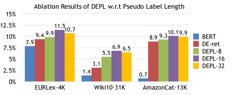
Figure 4: The ablation-test results of DEPL in Macro-averaged F1@k metric with varying length of pseudo label descriptions.

Table 6: Ablation-test results of DEPL under different training conditions.

Methods P@1 P@3 P@5 PSP@1 PSP@3 PSP@5 EUR-Lex DE-ret -1.34 -1.18 -1.16 -3.2 -2.11 +0.18 w/o pre-train -6.81 -6.72 -6.16 -6.87 -7.09 -5.87 w/o neg -2.52 -2.63 -2.2 -3.59 -3.66 -1.9 5 hard negative -1.55 -1.19 -1.12 -3.57 -2.98 -1.32 Wiki10-31K DE-ret -3.31 -7.35 -10.74 -5.43 -4.43 -4.55 w/o pre-train -4.72 -8.3 -10.9 -1.56 -1.36 -1.27 w/o hard negative -1.91 -5.54 -3.73 -0.25 -0.53 -0.72 5 hard negative -0.71 -2.77 -2.96 -0.32 -0.35 -0.27

6.3 Ablation Study

Pseudo Label Description

In figure 4, we conduct an ablation test on the length of the pseudo label and the performance is measured by Macro-avg F1@k. The BERT classifier is included as a baseline with no label text information (length equals $0$). As we observe that the longer description of length $16$ performs the better, but when length is $32$, the performance doesn’t increase as the text may become noisy with more unrelated keywords.

The DE-ret model is a pure retrieval baseline (avg length $3$) with only the label name. While it achieves good performance on the EURLex-4K and AmazonCat-13K datasets, it still performs poorly on the Wiki10-31K dataset. Another evidence is shown in table 6, where the performance of DE-ret drops more significantly on the Wiki10-31K dataset. That shows that generating the keywords from the sparse classifier can enhance the text quality. Furthermore, the generated text allows DEPL to use the semantic information of the label keywords, which is ignored in the SVM model. This could be another reason why our model performs better than the SVM baseline on the Wiki10-31K dataset.

In table 5, we pick the illustrative examples of the SVM generated keywords trained on the Wiki10-31K dataset for labels with only $1$ training example. We manually highlight the meaningful terms related to the label meaning. For example, the label name phase4 is ambiguous, whose meaning needs to be inferred from the corresponding document. From the keywords trial, clinical, drug …, we can understand it is about medical testing phase and the keywords can enhance the label semantic. In another example, kakuro is a Japanese logic puzzle known as a mathematical crossword and the game play involves in adding number in the cells. Generating a description for kakuro requires the background knowledge, but the keywords automatically learned from the sparse classifier provide the key concepts. Although not all the keywords can provide rich semantics to complement the original label name, they may serve as a context for the label to make it more distinguishable from others.

Model Pre-training

We fine-tune our retrieval model on a pre-trained neural classifier (BERT) and table 6 shows that without using the pre-trained model, there is a significant drop in the precision and PSP metrics.

Negative Sampling

We used the top negative predictions by the SVM model as the choice of hard negative labels. By default, we use $10$ hard negatives for each instance in the batch. In table 6, we observe a performance drop when no hard negatives or only $5$ hard negatives are used for training.

7 Conclusion

In this paper, we propose a novel neural retrieval framework (DEPL) for the open challenge of tail-label prediction in XMTC. By formulating the problem as to capture the semantic mapping between input documents and system-enhanced label descriptions, DEPL combines the strengths of neural embedding based retrieval and the effectiveness of a large-marge BoW classifier in generating informative label descriptions under severe data sparse conditions. Our extensive experiments on very large benchmark datasets show significant performance improvements by DEPL over strong baseline methods, especially in tail label description.

Appendix A Appendix

We include the assumptions and proofs of Theorem 3.

Assumptions

Similar to Luan et al. (2020), we treat neural embedding as fixed dense vector ${\bm{E}}\in\mathbb{R}^{d\times v}$ with each entry sampled from a random Gaussian $N(0,d^{-1/2})$. $\phi_{n}({\bm{x}})={\bm{E}}\phi_{t}({\bm{x}})$ is weighted average of word embeddings by the sparse vector representation of text. According to the Johnson-Lindenstrauss (JL) Lemma (Johnson and Lindenstrauss, 1984; Ben-David et al., 2002), even if the entries of ${\bm{E}}$ are sampled from a random normal distribution, with large probability, $\langle\phi_{t}({\bm{x}}),{\bm{v}}\rangle$ and $\langle{\bm{E}}\phi_{t}({\bm{x}}),{\bm{E}}{\bm{v}}\rangle$ are close.

Lemma 4.

Let ${\bm{v}}$ be the $\delta$-bounded keyword-selected label embedding of ${\bm{w}}$. For two labels $p,n$, the error margins satisfy:

$$|\mu(\phi_{t}({\bm{x}}),{\bm{w}}_{p},{\bm{w}}_{n})-\mu(\phi_{t}({\bm{x}}),{\bm{v}}_{p},{\bm{v}}_{n})|\leq\delta$$

Proof.

By the definition of $\delta$-bounded keywords,

$$\langle\phi_{t}({\bm{x}}),{\bm{w}}_{p}\rangle-\delta\leq\langle\phi_{t}({\bm{x}}),{\bm{v}}_{p}\rangle\leq\langle\phi_{t}({\bm{x}}),{\bm{w}}_{p}\rangle$$ (7)

$$-\langle\phi_{t}({\bm{x}}),{\bm{w}}_{n}\rangle\leq-\langle\phi_{t}({\bm{x}}),{\bm{v}}_{n}\rangle\leq-\langle\phi_{t}({\bm{x}}),{\bm{w}}_{n}\rangle+\delta$$ (8)

Adding equation 7 and equation 8 finishes the proof:

$$\langle\phi_{t}({\bm{x}}),{\bm{w}}_{p}-{\bm{w}}_{n}\rangle-\delta\leq\langle\phi_{t}({\bm{x}}),{\bm{v}}_{p}-{\bm{v}}_{n}\rangle\leq\langle\phi_{t}({\bm{x}}),{\bm{w}}_{p}-{\bm{w}}_{n}\rangle+\delta$$ (9)

∎

Lemma 5.

Let $\phi_{t}({\bm{x}})$ and $\phi_{n}({\bm{x}})$ be the sparse and dense (dimension $d$) document feature, ${\bm{w}}_{l}$ be the label embedding and ${\bm{z}}_{l}$ be the $\delta$-bounded keywords. Let $p$ be a positive label and $n$ be a negative label ranked below $p$ be the sparse classifier. The error margin is $\epsilon=\mu(\phi_{t}({\bm{x}}),{\bm{w}}_{p},{\bm{w}}_{n})$. An error ${\mathcal{E}}$ of neural classification occurs when $\mu(\phi_{n}({\bm{x}}),\phi_{n}({\bm{z}}_{p}),\phi_{n}({\bm{z}}_{n}))\leq 0$. The probability $P({\mathcal{E}})\leq 4\exp(-\frac{(\epsilon-\delta)^{2}d}{50})$.

Proof.

By the JL Lemma (Ben-David et al., 2002): For any two vectors ${\bm{a}},{\bm{b}}\in{\mathbb{R}}^{v}$, let ${\bm{E}}\in{\mathbb{R}}^{d\times v}$ be a random matrix such that the entries are sampled from a random Gaussian. Then for every constant $\gamma>0$:

$$P\left(|\langle{\bm{E}}{\bm{a}},{\bm{E}}{\bm{b}}\rangle-\langle{\bm{a}},{\bm{b}}\rangle|\geq\frac{\gamma}{2}\left(\|{\bm{a}}\|^{2}+\|{\bm{b}}\|^{2}\right)\right)\leq 4\exp\left(-\frac{\gamma^{2}d}{8}\right)$$ (10)

Let $\gamma=\frac{2}{5}(\epsilon-\delta)$, ${\bm{a}}=\phi_{t}({\bm{x}})$ and ${\bm{b}}={\bm{v}}_{p}-{\bm{v}}_{n}$. Since $\|{\bm{a}}\|_{2}=1$ and $\|{\bm{b}}\|_{2}\leq(\|{\bm{v}}_{p}\|_{2}+\|{\bm{v}}_{n}\|_{2})^{2}\leq 4$, the JL Lemma gives

$$P\left(|\langle{\bm{E}}\phi_{t}({\bm{x}}),{\bm{E}}({\bm{v}}_{p}-{\bm{v}}_{n})\rangle-\langle\phi_{t}({\bm{x}}),{\bm{v}}_{p}-{\bm{v}}_{n}\rangle|\geq\epsilon-\delta\right)$$ (11)

$$\leq 4\exp(-\frac{(\epsilon-\delta)^{2}d}{50})$$ (12)

To complete the proof, we need to show $P({\mathcal{E}})\leq Eq.\ref{eq:jl}$:

$${\mathcal{E}} \implies\quad |\langle{\bm{E}}\phi_{t}({\bm{x}}),{\bm{E}}({\bm{v}}_{p}-{\bm{v}}_{n})\rangle-\langle\phi_{t}({\bm{x}}),{\bm{w}}_{p}-{\bm{w}}_{n}\rangle| \geq\epsilon$$ (13)

$$\implies\quad |\langle{\bm{E}}\phi_{t}({\bm{x}}),{\bm{E}}({\bm{v}}_{p}-{\bm{v}}_{n})\rangle-\langle\phi_{t}({\bm{x}}),{\bm{v}}_{p}-{\bm{v}}_{n}\rangle| \geq\epsilon-\delta$$ (14)

where the equation 14 is derived by Lemma 4:

$$|\langle{\bm{E}}\phi_{t}({\bm{x}}),{\bm{E}}({\bm{v}}_{p}-{\bm{v}}_{n})\rangle-\langle\phi_{t}({\bm{x}}),{\bm{v}}_{p}-{\bm{v}}_{n}\rangle|$$ (15)

$$\geq |\langle{\bm{E}}\phi_{t}({\bm{x}}),{\bm{E}}({\bm{v}}_{p}-{\bm{v}}_{n})\rangle-\langle\phi_{t}({\bm{x}}),{\bm{w}}_{p}-{\bm{w}}_{n}\rangle|-$$ (16)

$$|\langle\phi_{t}({\bm{x}}),{\bm{w}}_{p}-{\bm{w}}_{n}\rangle-\langle\phi_{t}({\bm{x}}),{\bm{v}}_{p}-{\bm{v}}_{n}\rangle|$$ (17)

$$\geq \epsilon-\delta$$ (18)

Therefore $P({\mathcal{E}})\leq Eq.\ref{eq:jl}$, which completes the proof. ∎

Proof of Theorem 3

Proof.

The Lemma 2 shows that

$$P({\mathcal{E}}_{i})\leq 4\exp(-\frac{(\epsilon_{i}-\delta)^{2}d}{50})\leq 4\exp(-\frac{(\epsilon-\delta)^{2}d}{50})$$ (19)

By an union bound on the error events $\{{\mathcal{E}}_{1},{\mathcal{E}}_{2},\ldots,{\mathcal{E}}_{M_{p}}\}$,

$$P({\mathcal{E}}_{1}\cup\ldots\cup{\mathcal{E}}_{M_{p}}) \leq\sum_{i=1}^{M_{p}}4\exp(-\frac{(\epsilon_{i}-\delta)^{2}d}{50})$$ (20)

$$=4{M_{p}}\exp(-\frac{(\epsilon-\delta)^{2}d}{50})$$ (21)

∎

When $(\epsilon-\delta)^{2}\geq 10\sqrt{\frac{\log{M_{p}}}{d}}$, we have $\exp(-\frac{(\epsilon-\delta)^{2}d}{50})\leq\frac{1}{4{M_{p}}^{2}}$ and therefore $P({\mathcal{E}}_{1}\cup\ldots\cup{\mathcal{E}}_{M_{p}})\leq\frac{1}{{M_{p}}}$.

References

- (1)
- Babbar and Schölkopf (2017) Rohit Babbar and Bernhard Schölkopf. 2017. Dismec: Distributed sparse machines for extreme multi-label classification. In Proceedings of the Tenth ACM International Conference on Web Search and Data Mining. 721–729.
- Babbar and Schölkopf (2019) Rohit Babbar and Bernhard Schölkopf. 2019. Data scarcity, robustness and extreme multi-label classification. Machine Learning 108, 8 (2019), 1329–1351.
- Ben-David et al. (2002) Shai Ben-David, Nadav Eiron, and Hans Ulrich Simon. 2002. Limitations of learning via embeddings in Euclidean half spaces. Journal of Machine Learning Research 3, Nov (2002), 441–461.
- Chai et al. (2020) Duo Chai, Wei Wu, Qinghong Han, Fei Wu, and Jiwei Li. 2020. Description based text classification with reinforcement learning. In International Conference on Machine Learning. PMLR, 1371–1382.
- Chang et al. (2020) Wei-Cheng Chang, Hsiang-Fu Yu, Kai Zhong, Yiming Yang, and Inderjit S Dhillon. 2020. Taming pretrained transformers for extreme multi-label text classification. In Proceedings of the 26th ACM SIGKDD International Conference on Knowledge Discovery & Data Mining. 3163–3171.
- Dahiya et al. (2021) Kunal Dahiya, Ananye Agarwal, Deepak Saini, K Gururaj, Jian Jiao, Amit Singh, Sumeet Agarwal, Purushottam Kar, and Manik Varma. 2021. SiameseXML: Siamese Networks meet Extreme Classifiers with 100M Labels. In International Conference on Machine Learning. PMLR, 2330–2340.
- Devlin et al. (2018) Jacob Devlin, Ming-Wei Chang, Kenton Lee, and Kristina Toutanova. 2018. Bert: Pre-training of deep bidirectional transformers for language understanding. arXiv preprint arXiv:1810.04805 (2018).
- Gao and Callan (2021) Luyu Gao and Jamie Callan. 2021. Unsupervised corpus aware language model pre-training for dense passage retrieval. arXiv preprint arXiv:2108.05540 (2021).
- Gao et al. (2021) Luyu Gao, Zhuyun Dai, and Jamie Callan. 2021. COIL: Revisit Exact Lexical Match in Information Retrieval with Contextualized Inverted List. arXiv preprint arXiv:2104.07186 (2021).
- Gao et al. (2004) Luyu Gao, Zhuyun Dai, Tongfei Chen, Zhen Fan, BV Durme, and Jamie Callan. 2004. Complementing lexical retrieval with semantic residual embedding (2020). URL: http://arxiv. org/abs (2004).
- Gopal and Yang (2010) Siddharth Gopal and Yiming Yang. 2010. Multilabel classification with meta-level features. In Proceedings of the 33rd international ACM SIGIR conference on Research and development in information retrieval. 315–322.
- Gopal and Yang (2013) Siddharth Gopal and Yiming Yang. 2013. Recursive regularization for large-scale classification with hierarchical and graphical dependencies. In Proceedings of the 19th ACM SIGKDD international conference on Knowledge discovery and data mining. 257–265.
- Gopal et al. (2012) Siddarth Gopal, Yiming Yang, Bing Bai, and Alexandru Niculescu-Mizil. 2012. Bayesian models for large-scale hierarchical classification. (2012).
- Honnibal and Montani (2017) Matthew Honnibal and Ines Montani. 2017. spaCy 2: Natural language understanding with Bloom embeddings, convolutional neural networks and incremental parsing. (2017). To appear.
- Jain et al. (2019) Himanshu Jain, Venkatesh Balasubramanian, Bhanu Chunduri, and Manik Varma. 2019. Slice: Scalable linear extreme classifiers trained on 100 million labels for related searches. In Proceedings of the Twelfth ACM International Conference on Web Search and Data Mining. 528–536.
- Jain et al. (2016a) Himanshu Jain, Yashoteja Prabhu, and Manik Varma. 2016a. Extreme Multi-Label Loss Functions for Recommendation, Tagging, Ranking & Other Missing Label Applications. In Proceedings of the 22nd ACM SIGKDD International Conference on Knowledge Discovery and Data Mining.
- Jain et al. (2016b) Himanshu Jain, Yashoteja Prabhu, and Manik Varma. 2016b. Extreme multi-label loss functions for recommendation, tagging, ranking & other missing label applications. In Proceedings of the 22nd ACM SIGKDD International Conference on Knowledge Discovery and Data Mining. 935–944.
- Jiang et al. (2021) Ting Jiang, Deqing Wang, Leilei Sun, Huayi Yang, Zhengyang Zhao, and Fuzhen Zhuang. 2021. LightXML: Transformer with Dynamic Negative Sampling for High-Performance Extreme Multi-label Text Classification. arXiv preprint arXiv:2101.03305 (2021).
- Johnson and Lindenstrauss (1984) William B Johnson and Joram Lindenstrauss. 1984. Extensions of Lipschitz mappings into a Hilbert space 26. Contemporary mathematics 26 (1984).
- Karpukhin et al. (2020) Vladimir Karpukhin, Barlas Oğuz, Sewon Min, Patrick Lewis, Ledell Wu, Sergey Edunov, Danqi Chen, and Wen-tau Yih. 2020. Dense passage retrieval for open-domain question answering. arXiv preprint arXiv:2004.04906 (2020).
- Khandagale et al. (2019) Sujay Khandagale, Han Xiao, and Rohit Babbar. 2019. Bonsai – Diverse and Shallow Trees for Extreme Multi-label Classification. arXiv:1904.08249 [cs.LG]
- Lee et al. (2019) Jinhyuk Lee, Minjoon Seo, Hannaneh Hajishirzi, and Jaewoo Kang. 2019. Contextualized sparse representations for real-time open-domain question answering. arXiv preprint arXiv:1911.02896 (2019).
- Liu et al. (2017) Jingzhou Liu, Wei-Cheng Chang, Yuexin Wu, and Yiming Yang. 2017. Deep learning for extreme multi-label text classification. In Proceedings of the 40th International ACM SIGIR Conference on Research and Development in Information Retrieval. 115–124.
- Loza Mencía and Fürnkranz (2008) Eneldo Loza Mencía and Johannes Fürnkranz. 2008. Efficient Pairwise Multilabel Classification for Large-Scale Problems in the Legal Domain. In Machine Learning and Knowledge Discovery in Databases, Walter Daelemans, Bart Goethals, and Katharina Morik (Eds.). Springer Berlin Heidelberg.
- Luan et al. (2020) Yi Luan, Jacob Eisenstein, Kristina Toutanova, and Michael Collins. 2020. Sparse, dense, and attentional representations for text retrieval. arXiv preprint arXiv:2005.00181 (2020).
- McAuley and Leskovec (2013) Julian McAuley and Jure Leskovec. 2013. Hidden Factors and Hidden Topics: Understanding Rating Dimensions with Review Text. Association for Computing Machinery, 165–172. https://doi.org/10.1145/2507157.2507163
- Pedregosa et al. (2011) F. Pedregosa, G. Varoquaux, A. Gramfort, V. Michel, B. Thirion, O. Grisel, M. Blondel, P. Prettenhofer, R. Weiss, V. Dubourg, J. Vanderplas, A. Passos, D. Cournapeau, M. Brucher, M. Perrot, and E. Duchesnay. 2011. Scikit-learn: Machine Learning in Python. Journal of Machine Learning Research 12 (2011), 2825–2830.
- Prabhu et al. (2018) Yashoteja Prabhu, Anil Kag, Shrutendra Harsola, Rahul Agrawal, and Manik Varma. 2018. Parabel: Partitioned label trees for extreme classification with application to dynamic search advertising. In Proceedings of the 2018 World Wide Web Conference. 993–1002.
- Wei et al. (2021) Tong Wei, Wei-Wei Tu, Yu-Feng Li, and Guo-Ping Yang. 2021. Towards Robust Prediction on Tail Labels. In Proceedings of the 27th ACM SIGKDD Conference on Knowledge Discovery & Data Mining. 1812–1820.
- Xiong et al. (2020) Lee Xiong, Chenyan Xiong, Ye Li, Kwok-Fung Tang, Jialin Liu, Paul Bennett, Junaid Ahmed, and Arnold Overwijk. 2020. Approximate nearest neighbor negative contrastive learning for dense text retrieval. arXiv preprint arXiv:2007.00808 (2020).
- Yang and Liu (1999) Yiming Yang and Xin Liu. 1999. A re-examination of text categorization methods. In Proceedings of the 22nd annual international ACM SIGIR conference on Research and development in information retrieval. 42–49.
- Ye et al. (2020) Hui Ye, Zhiyu Chen, Da-Han Wang, and Brian Davison. 2020. Pretrained Generalized Autoregressive Model with Adaptive Probabilistic Label Clusters for Extreme Multi-label Text Classification. In International Conference on Machine Learning. PMLR, 10809–10819.
- Yen et al. (2017) Ian EH Yen, Xiangru Huang, Wei Dai, Pradeep Ravikumar, Inderjit Dhillon, and Eric Xing. 2017. Ppdsparse: A parallel primal-dual sparse method for extreme classification. In Proceedings of the 23rd ACM SIGKDD International Conference on Knowledge Discovery and Data Mining. 545–553.
- You et al. (2018) Ronghui You, Zihan Zhang, Ziye Wang, Suyang Dai, Hiroshi Mamitsuka, and Shanfeng Zhu. 2018. Attentionxml: Label tree-based attention-aware deep model for high-performance extreme multi-label text classification. arXiv preprint arXiv:1811.01727 (2018).
- Zubiaga (2012) Arkaitz Zubiaga. 2012. Enhancing Navigation on Wikipedia with Social Tags. arXiv:1202.5469 [cs.IR]