Finding the Nearest Negative Imaginary System with Application to Near-Optimal Controller Design

Abstract

The negative imaginary (NI) systems theory has attracted interests due to the robustness properties of feedback interconnected NI systems. However, a full output optimal controller-synthesis methodology, for such class of systems, is yet to exist. In order to develop a solution towards this problem, we first develop a methodology to find the nearest NI system to a non NI system. This later problem stated as follows: for any linear time invariant (LTI) system defined by the state space matrices $(A,B,C,D)$, find the nearest NI system, with the state space matrices $(A+\Delta_{A},B+\Delta_{B},C+\Delta_{C},D+\Delta_{D})$, such that the norm of $(\Delta_{A},\Delta_{B},\Delta_{C},\Delta_{D})$ is minimized. Then, this methodology will be used to find the nearest optimal controller for a given NI plant. In other words, for a given NI system, an optimal control methodology, such as LQG, is used to design an optimal controller that satisfy a particular performance measure. Then, the developed methodology of finding the nearest NI system is used, as a near-optimal control synthesis methodology, to find the nearest NI system to the designed optimal controller. Hence, the synthesized controller satisfy the NI property and therefore guarantee a robust feedback loop with the negative imaginary system under control.

I INTRODUCTION

Dynamical systems with flexibly structured dynamics exists in many important engineering systems. For instance, in aerospace systems [1, 2], robot manipulators [3], atomic force microscopes (AFMs) [4, 5], and other nano-positioning systems [6, 7]). The common physical structure between these systems is the involvement of a combination of force actuators and sensors. These systems are susceptible to changes in environmental variables. For instance, the existence of the highly resonant modes in these flexible systems can affect robustness and stability characteristics [8, 9, 10]. Relatively small stimuli or perturbations in the environment, such as changing temperature, can lead to significant impacts in the systems’ resonant frequencies. These changes in resonant frequencies result in changes in the system’s phase and gain at a given frequency, which can easily lead to unacceptable behavior, such as instability or poor performance in the system. Moreover, these dynamical systems, by their nature, are infinite-dimensional systems [8, 11, 12], which are hard to model and control. Instead, finite-dimensional models are used as approximation models to be used in controller synthesis [8].

Negative imaginary (NI) systems theory represent an important class of these flexibly structure dynamics systems [13, 10, 14, 15, 16, 17, 18], In particular, flexible structure dynamics when a force actuator is combined with a collocated, position or acceleration, sensor are known to satisfy the NI property.

The NI propriety can be defined, in the case of the single-input single-output (SISO), based on the properties of the imaginary part of the complex function of the frequency response $G(j\omega)$. This is,

$$j\left(G(j\omega)-G(j\omega)^{\ast}\right)\geq 0,$$

to be satisfied for all $\omega\in(0,\infty)$. A formal definition of NI system is given in the next section .

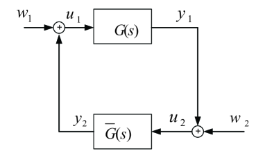
Figure 1: A negative-imaginary feedback control system.

A fundamental result of NI systems theory is concerning the feedback of interconnected NI systems. That is, the closed feedback interconnection between an NI system and strictly negative imaginary, as shown in Fig. 1, is stable under a given DC gain condition. This result made the NI theory attractive to be used in controller design, i.e., if the system under control satisfy the NI property, one can design an NI controller so that the robust stability is guaranteed for free. This led to several attempts to synthesis an NI controller that preserve certain performance measures [19, 10, 20, 21, 22]. However, a full output optimal controller for an NI system is yet to exist. One aim of this paper is to present a near-optimal control synthesis methodology for negative imaginary systems. The synthesized controller satisfies the NI property, and therefore, guarantee a robust feedback loop with the negative imaginary system under control.

In order to develop the near-optimal control methodology, we first develop a method to find the nearest NI system for any non-NI system. In other words, given an LTI system, minimize the Frobenius norm of $(\Delta_{A},\Delta_{B},\Delta_{C},\Delta_{D})$ such that $(A+\Delta_{A},B+\Delta_{B},C+\Delta_{C},D+\Delta_{D})$ satisfies the NI property. The problem of finding the nearest negative imaginary system is motivated by a similar problem of finding the nearest positive real system (passive system) presented in [23, 24, 25, 26, 27]. In [25], several assumptions, such as $D+D^{T}$ to be non-singular are made. Also, they restrict the perturbation on the matrix $C$ only. The methods in [26] and [27] they perturb, both, $B$ and/or $C$. In [28], perturbations in all system matrices. Similar results for NI system were developed in [29] where an algorithm was developed for enforcing negative imaginary property in case of any violation during system identifications. This assumes that the underlying dynamics ought to belong to negative imaginary system class. The method is based on the spectral properties of Hamiltonian matrices.

In this paper, we use the result developed in [23] to develop similar results of finding the nearest negative imaginary system. One of the main advantages of this method over the other perturbation methods is that there are no assumptions in the system. Also, in the positive real case, it allows for perturbations of all system matrices $(A,B,C,D)$.

The developed method of finding the nearest NI system will be used in order to find a near-optimal NI controller for a given NI plant. We first use a regular optimal control methodology such as LQG to design an optimal controller for a given NI system. Then, we employ the developed method of the nearest NI dynamical system to find the NI optimal controller.

As discussed, there are two main contributions in this paper, which can be summarized as follows:

1. First, the paper introduces a methodology for finding the nearest negative imaginary system for a non-negative imaginary system. The proposed method is based on the Port-Hamiltonian formulation of the negative imaginary systems.

2. Second, these result of finding the nearest negative imaginary system will be used in order to find the nearest NI optimal controller for a given negative imaginary plant. The synthesized controller satisfies a near optimal performance with the negative imaginary robustness property.

II Preliminaries

In this section, we present the definitions and lemmas of the negative imaginary systems. Also, this section presents the Port-Hamiltonian formulation of the negative imaginary systems.

II-A Negative imaginary systems

In this section, we recall the definition of linear time invariant (LTI) negative imaginary systems as given in [15].

Consider the following LTI system defined in (1)

$$\begin{split}\dot{x}(t)=&Ax(t)+Bu(t),\\ y(t)=&\;Cx(t)+Du(t),\end{split}$$ (1)

where, $A$ represents the dynamical matrix with dominion belongs to $\mathbb{R}^{n\times n}$, $B$ is the input matrix $\in\mathbb{R}^{n\times m}$, $C$ represents the output matrix $\in\mathbb{R}^{m\times n},$ and $D\in\mathbb{R}^{m\times m}.$ This yields a transfer function matrix $G(s)=C(sI-A)^{-1}B+D$. The transfer function matrix $G(s)$ is said to be strictly proper if $G(\infty)=D=0$. The notation $\begin{bmatrix}\begin{array}[]{c|c}A&B\\ \hline\cr C&D\end{array}\end{bmatrix}$ will be used to denote the state space realization (1).

The NI system is formally defined in [15].

Definition 1

[15] A square transfer function matrix $G(s)$ is NI if the following conditions are satisfied:

1. $G(s)$ has no pole in $Re[s]>0$.

2. For all $\omega>0$ such that $s=j\omega$ is not a pole of $G(s)$,

   $$j\left(G(j\omega)-G(j\omega)^{\ast}\right)\geq 0.$$ (2)

3. If $s=j\omega_{0}$ with $\omega_{0}>0$ is a pole of $G(s)$, then it is a simple pole and the residue matrix $K=\underset{s\longrightarrow j\omega_{0}}{\lim}(s-j\omega_{0})jG(s)$ is Hermitian and positive semidefinite.

4. If $s=0$ is a pole of $G(s)$, then $\underset{s\longrightarrow 0}{\lim}s^{k}G(s)=0$ for all $k\geq 3$ and $\underset{s\longrightarrow 0}{\lim}s^{2}G(s)$ is Hermitian and positive semidefinite.

Definition 2

[30] A square transfer function matrix $G(s)$ is SNI if the following conditions are satisfied:

1. ${G}(s)$ has no pole in $Re[s]\geq 0$.

2. For all $\omega>0$, $j\left({G}(j\omega)-{G}(j\omega)^{\ast}\right)>0$.

Here, we present an NI lemma.

Lemma 1

Let $\begin{bmatrix}\begin{array}[]{c|c}A&B\\ \hline\cr C&D\end{array}\end{bmatrix}$ defining the system (LABEL:eq:xdotn)-(LABEL:eq:yn) be a minimal realization of the transfer function matrix $G(s)$. Then, $G(s)$ is NI if and only if $D=D^{T}$ and there exist matrices $P=P^{T}\geq 0$, $W\in\mathbb{R}^{m\times m}$, and $L\in\mathbb{R}^{m\times n}$ such that the following linear matrix inequality (LMI) is satisfied:

$$\begin{bmatrix}PA+A^{T}P&PB-A^{T}C^{T}\\ B^{T}P-CA&-(CB+B^{T}C^{T})\end{bmatrix}=\begin{bmatrix}-L^{T}L&-L^{T}W\\ -W^{T}L&-W^{T}W\end{bmatrix}\leq 0.$$ (3)

A state-space characterization of NI systems in terms of a pair of linear matrix inequalities (LMIs) has been given in [13]. This result also generalized in [30] to include poles on the imaginary axis except at the origin.

Lemma 2

(See [30]) Let $\begin{bmatrix}\begin{array}[]{c|c}A&B\\ \hline\cr C&D\end{array}\end{bmatrix}$ be a minimal state space realization of a transfer function matrix $G(s)$. Then $G(s)$ is NI if and only if $det(A)\neq 0$, $D=D^{T}$ and there exists a real matrix $Y>0$ such that

$$AY+YA^{*}\leq 0\ \text{and}\ B=-AYC^{*}.$$ (4)

Lemma 3

Let $\begin{bmatrix}\begin{array}[]{c|c}A&B\\ \hline\cr C&D\end{array}\end{bmatrix}$ be a minimal realization of the transfer function matrix $G(s)$ for the system in (1). Then, $G(s)$ is NI if and only if $D=D^{T}$ and there exists a matrix $P=P^{T}\geq 0$ such that the following LMI is satisfied:

$$\begin{bmatrix}PA+A^{T}P&PB-A^{T}C^{T}\\ B^{T}P-CA&-(CB+B^{T}C^{T})\end{bmatrix}\leq 0.$$ (5)

Furthermore, if $G(s)$ is SNI, then $\det(A)\neq 0$ and there exists a matrix $P>0$ such that (5) holds.

One of the important results in the NI system’s theory is the robustness property that emerge in the case of positive feedback interconnection between an NI and an SNI system as shown in Fig. 1. The following theorem form [10, 13] states this results:

Theorem 1

Consider an NI transfer function matrix $G(s)$ with no poles at the origin and an SNI transfer function matrix $\bar{G}(s)$, and suppose that $G(\infty)\bar{G}(\infty)=0$ and $\bar{G}(\infty)\geq 0$. Then, the positive-feedback interconnection (see Fig. 1) of $G(s)$ and $\bar{G}(s)$ is internally stable if and only if $\lambda_{max}(G(0)\bar{G}(0))<1$.

The above Theorem 1 characterizes the conditions of the stability of the feedback interconnection of two NI and SNI systems through the phase stabilization.

II-B Port-Hamiltonian formulation of negative imaginary systems

To establish the results in this paper, the formulation of the negative imaginary system is used. Port-Hamiltonian formulation of negative imaginary systems was developed in [31, 32]. The following lemma characterize the NI systems as a Port-Hamiltonian system.

Lemma 4

The system given in (1) has negative imaginary transfer function if and only if it can be written as

$$\begin{split}\dot{x}(t)=&\;(J-R)Q(x(t)-C^{T}u(t)),\\ y(t)=&\;Cx(t)+Du(t),\end{split}$$ (6)

for some matrices $Q,J,R$, where,

$$Q=Q^{T}>0,\ \ \ J=-J^{T},\ \ \ R=R^{T}\geq 0.$$ (7)

The proof is the same as proposition (2.4) in [31].

The above lemma be our main tool to reformulate the nearest negative imaginary system problem. The next sections will focus on defining the problem formulation.

III Main results

In this section, we present the main results in this paper.

III-A Nearest negative imaginary system problems

As indicated in the introduction, the problem of finding the nearest negative imaginary system is similar to the problem of finding the nearest positive real system (passive system) presented in [23], where the port-Hamiltonian formulation is used.

Let us now define the nearest negative imaginary system problems under consideration:

Problem 1

Suppose an LTI system with the following state space representation $\begin{bmatrix}\begin{array}[]{c|c}A&B\\ \hline\cr C&D\end{array}\end{bmatrix}$, find the nearest (the closest) system $\begin{bmatrix}\begin{array}[]{c|c}\tilde{A}&\tilde{B}\\ \hline\cr\tilde{C}&\tilde{D}\end{array}\end{bmatrix},$ such that,

$$\inf_{(\tilde{A},\tilde{B},\tilde{C},\tilde{D})}\mathcal{F}(\tilde{A},\tilde{B},\tilde{C},\tilde{D}),$$

where,

$$\mathcal{F}(\tilde{A},\tilde{B},\tilde{C},\tilde{D})= {\|A-\tilde{A}\|}_{F}^{2}+{\|B-\tilde{B}\|}_{F}^{2}$$

$$+{\|C-\tilde{C}\|}_{F}^{2}+{\|D-\tilde{D}\|}_{F}^{2}.$$ (8)

The following definition is based on Lemma 4 and compares the system descried in (6) with the LTI system given in (1).

Definition 3

A system $(A,B,C,D)$ is said to admit a port-Hamiltonian form if there exists a system as defined in (6) such that

$$A=(J-R)Q,\text{ and},B=-(J-R)C^{T}$$

Based on the above definition, the problem given in (1) can be reduced to the following problem:

Problem 2

Suppose an LTI system with the following state space representation $\begin{bmatrix}\begin{array}[]{c|c}A&B\\ \hline\cr C&D\end{array}\end{bmatrix}$, find the nearest (the closest) system $\begin{bmatrix}\begin{array}[]{c|c}\tilde{A}&\tilde{B}\\ \hline\cr\tilde{C}&\tilde{D}\end{array}\end{bmatrix},$ such that,

$$\inf_{(\tilde{A},\tilde{B},\tilde{C},\tilde{D})}\mathcal{F}(\tilde{A},\tilde{B},\tilde{C},\tilde{D}),$$

where,

$$\mathcal{F}(\tilde{A},\tilde{B})={\|A-(J-R)Q\|}_{F}^{2}+{\|B-(R-J)C^{T}\|}_{F}^{2},$$ (9)

where, $\tilde{A}=(J-R)Q,\ \ \tilde{B}=-(J-R)C^{T}$.

III-B Algorithmic for nearest negative imaginary system problem

This section proposes an algorithm to solve the problem dissuaded in the above section.

The problem (2) can be written as follows

$$\inf_{J,R,Q} {\|A-(J-R)Q\|}_{F}^{2}+{\|B-(R-J)Q\|}_{F}^{2},$$

$$\text{ such that }J^{T}=-J,Q=Q^{T}>0,\text{and }R^{T}=R\geq 0.$$ (10)

The projected gradient method (FGM) presented in [33] and in [23] is used to solve the problem in  (10).

As indicated in [23], the projected gradient method is much faster and hence better to use compared to the standard projected gradient method [34].

The steps can be summarized as follows:

• Compute the gradient as follows:

  $${\|A-(J-R)Q\|}_{F}^{2}\Rightarrow\nabla_{J_{1}}=-2Q{\|A-(J-R)Q\|},$$

  $${\|A-(J-R)Q\|}_{F}^{2}\Rightarrow\nabla_{R_{1}}=2Q{\|A-(J-R)Q\|},$$

  $${\|A-(R-J)C^{T}\|}_{F}^{2}\Rightarrow\nabla_{J_{2}}=2C^{T}{\|A-(R-J)C^{T}\|},$$

  $${\|A-(R-J)C^{T}\|}_{F}^{2}\Rightarrow\nabla_{R_{2}}=-2C^{T}{\|A-(R-J)C^{T}\|},$$

  $${\|A-(J-R)Q\|}_{F}^{2}\Rightarrow\nabla_{Q}=-2(J-R){\|A-(J-R)Q\|},$$

  or simply, for a given term in the objective function, $f(X)={\|AX-B\|}_{F}^{2}$ the gradient is $\nabla_{Y}f(Y)=2A^{T}(AY-B)$.

• Project onto the feasible set of matrices $Q,R$ that satisfy both conditions, $Q=Q^{T}>0,\text{and }R^{T}=R\geq 0$.

The FGM Algorithm, which presented in [23], is used to compute the matrices $Q,R$.

Similar to the implementation in [23], positive weights $w_{i}$ were added to the objective function terms in order to give opportunity for a different importance of each term if needed. Therefore, the objective function can be written as follows:

$$\mathcal{F}(\tilde{A},\tilde{B})=w_{1}{\|A-(J-R)Q\|}_{F}^{2}+w_{2}{\|B-(R-J)C^{T}\|}_{F}^{2}.$$

Parameter settings in our implementation are similar to the parameter settings that was used in [23]. For instance, the step length is calculated as $\gamma=1/L$ where $L={\|Q\|}_{2}^{2}$. Moreover, in the initialization step, two different initializations were used.

The first initialization,

$$Q=I_{n},\ \ \ \ \ J=\big{(}A-A^{T}\big{)}/2,\ \ \ \ R=P_{>0}\big{(}(-A-A^{T})/2\big{)},$$

where the notation $\mathcal{P}_{>0}(X)$ stands for the projection of a matrix $X$ on the cone of positive semi-definite matrices.

LMI-based initialization: Since the given system is not an NI system, the LMI given in (5) has no solution. However, a solution $P$ to nearby LMIs should be a good initialization to the matrix $Q$. We propose the following to relax the LMIs (5):

$$\min_{\delta,P}\quad\delta^{2}$$

such that

$$\begin{bmatrix}-PA-A^{T}P&-PB+A^{T}C^{T}\\ -B^{T}P+CA&(CB+B^{T}C^{T})\end{bmatrix}+\delta I_{n+m}\geq 0,$$ (11)

III-C Optimal control design

In this section, the nearest NI problem, which was presented in the previous subsection, will be used in order to design a near-optimal controller for a given NI plant.

Suppose that we want to design a controller for a given NI plant, $G(s)$, with the state space representation given in (1). Suppose also that we decided to use any standard control synthesis methodology such as LQG or $H_{\infty}$ to design a controller that satisfy a particular performance measure. It is unlikely that the designed controller will satisfy the NI property and therefore, a robustness property will not be guaranteed. Hence, we can use the nearest NI problem, which was presented in the previous subsection, to find the nearest NI controller to the designed one. The following steps summarize the NI-control design, assuming that an LGQ is used in the design.

• Given an LTI NI plant in the form (1), with the transfer function matrix $G(s)=C(sI-A)^{-1}B+D$.

• Design a linear quadratic Gaussian (LQG) controller $K(s)=C_{c}(sI-A_{c})^{-1}B_{c}+D_{c}$, which minimizes the following cost function:

  $$J(u)=\int_{0}^{\infty}\left\{x^{T}Q_{c}x+2x^{T}N_{c}u+u^{T}R_{c}u\right\}dt.$$ (12)

• Use the methodology presented in this paper to find the nearest NI controller $\bar{G}(s)=\bar{C}(sI-\bar{A})^{-1}\bar{B}+\bar{D},$ to the designed LQG controller $K(s)$.

The new modified controller $\bar{G}(s)$ is a near-optimal controller that satisfy the NI property.

Remark 1

The DC gain condition $\lambda_{max}(G(0)\bar{G}(0))<1,$ can be included in the optimization process of finding the nearest NI controller. The DC gain of the NI controller can be calculated as follows:

$$\bar{G}(0)= -\bar{C}(\bar{A})^{-1}\bar{B}+\bar{D},$$

$$= \ \bar{C}((J-R)Q)^{-1}(J-R)\bar{C}^{T}+\bar{D},$$

$$= \ \bar{C}Q^{-1}\bar{C}^{T}+\bar{D}.$$

In the iterations of finding the matrix $Q$, particularly, in the projection iteration, the matrix $Q$ is scaled to satisfy the DC gain condition. The scaling factor that preserve the DC gain condition is:

$$Q_{new}=\alpha Q_{old}$$

where in the single-input single-output case,

$$\alpha=(CQ^{-1}_{old}C^{T}+D)G(0)+\epsilon,$$

with a small $\epsilon>0$.

IV Example

In this section, we present an example to illustrate the design approach presented in this paper.

It is well known that mechanical structures with colocated force actuators and position sensors yield negative imaginary systems [10]. Naturally, these systems are infinite dimension systems, whereas their models are not. This make the control design for such systems challenging. Particularly, in the case where the synthesis methodology do not take into account the robustness issue. Therefore, our method shows a big advantage over optimal control methodologies.

To illustrate this fact, consider the following lightly damped flexible structure LTI second-order system with a colocated force actuation and position measurement with the following structure:

$$G(s)=\sum_{n=1}^{N}\frac{1}{s^{2}+2\zeta_{n}\omega_{n}s+\omega_{n}^{2}},$$ (13)

where $\omega_{n}$ is the natural frequency and $\zeta_{n}$ the damping factor. Suppose that we want to design an LQG controller for the system given in (13). Since this model represents an infinite dimension system, a finite model is chosen to design the controller. We chose $N=2$ with $\omega_{1}=2,\omega_{2}=4$ and $\zeta_{1}=\zeta_{2}=0.02$ for the model parameters. This implies that the model gives the transfer function given in Fig. 2.

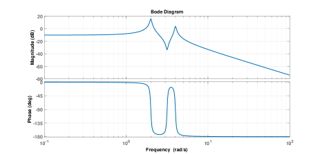
Figure 2: Bode plot of NI system given in (13), where N=2

With an appropriate LQG parameters, the controller is given as follows:

$$LQG(s)=\frac{-1.593s^{3}+9.84s^{2}-12.58s+93.76}{s^{4}+3.847s^{3}+26.66s^{2}+46.86s+125.1}.$$ (14)

The bode plot of the designed LGQ controller as given in 3 shows that it is not an NI controller, since the phase is not in the $(0,-\pi)$.

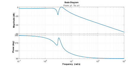
Figure 3: Bode plot of designed LQG controller given in (14)

Now, applying our method of finding the nearest NI controller to the LQG controller given in (14), we get the following transfer function,

$$NILQG(s)=\frac{13.75s^{2}+6.77s+132.5}{s^{4}+3.847s^{3}+26.66s^{2}+46.86s+125.1}$$ (15)

The bode plot in Fig. 4 of the controller given in (15) shows that it satisfy the NI property.

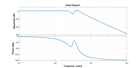
Figure 4: Bode plot of designed LQG controller given in (14)

Applying FGM on with the standard initialization, This gives a nearby standard NI system with error

$${\|A-\hat{A}\|}_{F}^{2}+{\|B-\hat{B}\|}_{F}^{2}+{\|C-\hat{C}\|}_{F}^{2}+{\|D-\hat{D}\|}_{F}^{2}=0.6430.$$

In terms of relative error for each matrix, we have

$$\frac{{\|A-\hat{A}\|}_{F}}{{\|A\|}_{F}}=5.5917e^{-18}\%,~{}\frac{{\|B-\hat{B}\|}_{F}}{{\|B\|}_{F}}=0.0631\%,~{}$$

$$\frac{{\|C-\hat{C}\|}_{F}}{{\|C\|}_{F}}=0\%,~{}\frac{{\|D-\hat{D}\|}_{F}}{{\|D\|}_{F}}=0\%.$$

The step response of the closed feedback interconnection of the plant given in (13) and both the designed LQG (14) controller and the nearest NI controller (15) are given in Fig. 5. It is clear that the response is very similar.

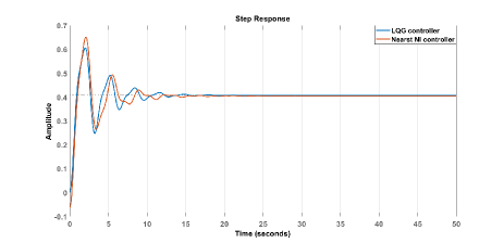
Figure 5: Bode plot of NI system given in (13), where N=2

The more interesting part of this example is when we add more non-modeled modes to the plant, i.e., $N=5$ as shown in Fig. 6 for instance. This means that we include some of the un-modulated dynamics in the plant, which was regarded as uncertainty. For instance, suppose that the plant

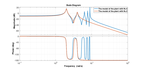
Figure 6: Bode plot of the plant model given in (13), with different numbers modes

As shown in Fig. 7, the designed LGQ (14) will become unstable if we considered the five-mode plant. However, the nearest NI controller still stabilize the system with an acceptable performance. This is due to the negative imaginary property of both, the controller and the plant.

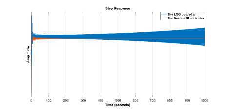
Figure 7: The step response of the designed LGQ (14) and the nearest NI controller plant model given in (13), with N=5

References

- [1] M. Harigae, I. Yamaguchi, T. Kasai, H. Igawa, and T. Suzuki, “Control of large space structures using GPS modal parameter identification and attitude and deformation estimation,” Electronics and Communications in Japan, vol. 86, no. 4, pp. 63–71, 2003.
- [2] V. P. Tran, M. Garratt, and I. R. Petersen, “Formation control of multi-uavs using negative-imaginary systems theory,” in 2017 11th Asian Control Conference (ASCC), pp. 2031–2036, IEEE, 2017.
- [3] D. G. Wilson, R. D. Robinett, G. G. Parker, and G. P. Starr, “Augmented sliding mode control for flexible link manipulators,” Journal of Intelligent and Robotic Systems, vol. 34, no. 4, pp. 415–430, 2002.
- [4] B. Bhikkaji and S. Moheimani, “Fast scanning using piezoelectric tube nanopositioners: A negative imaginary approach,” in Proc. IEEE/ASME Int. Conf. Advanced Intelligent Mechatronics AIM, (Singapore), pp. 274–279, July 2009.
- [5] I. A. Mahmood, S. O. R. Moheimani, and B. Bhikkaji, “A new scanning method for fast atomic force microscopy,” IEEE Transactions on Nanotechnology, vol. 10, no. 2, pp. 203–216, 2011.
- [6] S. Devasia, E. Eleftheriou, and S. O. R. Moheimani, “A survey of control issues in nanopositioning,” IEEE Transactions on Control Systems Technology, vol. 15, no. 5, pp. 802–823, 2007.
- [7] I. M. Diaz, E. Pereira, and P. Reynolds, “Integral resonant control scheme for cancelling human-induced vibrations in light-weight pedestrian structures,” Structural Control and Health Monitoring, vol. 19, no. 1, pp. 55–69, 2012.
- [8] A. Preumont, Vibration Control of Active Structures: An Introduction. Springer, 2011.
- [9] J. L. Fanson and T. K. Caughley, “Positive position feedback control for large space structures,” AIAA Journal, vol. 28, pp. 717–724, Apr. 1990.
- [10] I. R. Petersen and A. Lanzon, “Feedback control of negative imaginary systems,” IEEE Control System Magazine, vol. 30, no. 5, pp. 54–72, 2010.
- [11] K. Morris and F. Sciences, Control of Flexible Structures. Fields Institute communications, American Mathematical Society, 1993.
- [12] W. Ray, “Some recent applications of distributed parameter systems theory-a survey,” Automatica, vol. 14, no. 3, pp. 281 – 287, 1978.
- [13] A. Lanzon and I. R. Petersen, “Stability robustness of a feedback interconnection of systems with negative imaginary frequency response,” IEEE Transactions on Automatic Control, vol. 53, no. 4, pp. 1042–1046, 2008.
- [14] M. A. Mabrok, A. G. Kallapur, I. R. Petersen, and A. Lanzon, “Stabilization of conditional uncertain negative-imaginary systems using Riccati equation approach,” in 20th International Symposium on Mathematical Theory of Networks and Systems, 2012.
- [15] M. Mabrok, A. Kallapur, I. Petersen, and A. Lanzon, “Generalizing negative imaginary systems theory to include free body dynamics: Control of highly resonant structures with free body motion,” Automatic Control, IEEE Transactions on, vol. 59, pp. 2692–2707, Oct 2014.
- [16] A. Ferrante, A. Lanzon, and L. Ntogramatzidis, “Foundations of negative imaginary systems theory and relations with positive real systems,” arXiv preprint arXiv:1412.5709, 2014.
- [17] M. A. Mabrok, M. Efatmaneshnik, and M. Ryan, “Including non-functional requirements in the axiomatic design process,” in Systems Conference (SysCon), 2015 9th Annual IEEE International, pp. 54–60, IEEE, 2015.
- [18] M. Mabrok, M. Haggag, and I. Petersen, “System identification algorithm for negative imaginary systems,” International Journal of Applied and Computational Mathematics, vol. 14, no. 3, 2015.
- [19] I. R. Petersen, A. Lanzon, and Z. Song, “Stabilization of uncertain negative-imaginary systems via state-feedback control,” in Proceedings of the European Control Conference, (Budapest, Hungary), August 2009.
- [20] J. Xiong, J. Lam, and I. R. Petersen, “Output feedback negative imaginary synthesis under structural constraints,” Automatica, vol. 71, pp. 222–228, 2016.
- [21] M. A. Mabrok and I. R. Petersen, “Controller synthesis for negative imaginary systems: a data driven approach,” IET Control Theory & Applications, vol. 10, no. 12, pp. 1480–1486, 2016.
- [22] M. Mabrok, “Controller synthesis for negative imaginary systems using nonlinear optimisation and h 2 performance measure,” International Journal of Control, pp. 1–9, 2019.
- [23] N. Gillis and P. Sharma, “Finding the nearest positive-real system,” SIAM Journal on Numerical Analysis, vol. 56, no. 2, pp. 1022–1047, 2018.
- [24] A. Fazzi, N. Guglielmi, and C. Lubich, “Finding the nearest passive or nonpassive system via hamiltonian eigenvalue optimization,” SIAM Journal on Matrix Analysis and Applications, vol. 42, no. 4, pp. 1553–1580, 2021.
- [25] C. Schröder and T. Stykel, “Passivation of LTI systems,” tech. rep., Preprint, 368, 2007.
- [26] Y. Wang, Z. Zhang, C. Koh, G. Pang, and N. Wong, “PEDS: Passivity enforcement for descriptor systems via Hamiltonian-symplectic matrix pencil perturbation,” in, vol. 2010, pp. 800–807, 2010.
- [27] M. Voigt and P. Benner, Passivity enforcement of descriptor systems via structured perturbation of Hamiltonian matrix pencils. Linz: in Talk at Meeting of the GAMM Activity Group Dynamics and Control Theory, 2011.
- [28] T. Brull and C. Schröder, “Dissipativity enforcement via perturbation of para-Hermitian pencils,” IEEE Transactions on Circuits and Systems I: Regular Papers, vol. 60, pp. 164–177, 2013.
- [29] M. A. Mabrok, A. Lanzon, A. G. Kallapur, and I. R. Petersen, “Enforcing negative imaginary dynamics on mathematical system models,” International Journal of Control, vol. 86, no. 7, pp. 1292–1303, 2013.
- [30] J. Xiong, I. R. Petersen, and A. Lanzon, “A negative imaginary lemma and the stability of interconnections of linear negative imaginary systems,” IEEE Transactions on Automatic Control, vol. 55, no. 10, pp. 2342–2347, 2010.
- [31] A. Van der Schaft, “Positive feedback interconnection of hamiltonian systems.,” in CDC/ECC, pp. 6510–6515, 2011.
- [32] A. van der Schaft, “Interconnections of input-output hamiltonian systems with dissipation,” in 2016 IEEE 55th Conference on Decision and Control (CDC), pp. 4686–4691, IEEE, 2016.
- [33] N. Gillis and P. Sharma, “On computing the distance to stability for matrices using linear dissipative Hamiltonian systems,” Automatica, vol. 85, pp. 113–121, 2017.
- [34] Y. Nesterov, “A method of solving a convex programming problem with convergence rate o(1/k2),” Soviet Mathematics Doklady, vol. 27, pp. 372–376, 1983.