Exploiting Local and Global Features in Transformer-based
Extreme Multi-label Text Classification

Abstract

Extreme multi-label text classification (XMTC) is the task of tagging each document with the relevant labels from a very large space of predefined categories. Recently, large pre-trained Transformer models have made significant performance improvements in XMTC, which typically use the embedding of the special CLS token to represent the entire document semantics as a global feature vector, and match it against candidate labels. However, we argue that such a global feature vector may not be sufficient to represent different granularity levels of semantics in the document, and that complementing it with the local word-level features could bring additional gains. Based on this insight, we propose an approach that combines both the local and global features produced by Transformer models to improve the prediction power of the classifier. Our experiments show that the proposed model either outperforms or is comparable to the state-of-the-art methods on benchmark datasets.

1 Introduction

Extreme multi-label text classification (XMTC) is the task of tagging each document with relevant labels where the target space may contains up to thousands of category labels. Those labels typically form a semantic hierarchy, where the higher-level labels correspond to more abstract or general concepts, while the lower-level labels specify fine-grained distinctions. XMTC has many real-world applications, such as assigning subject topics to news or Wikipedia articles, tagging keywords for online shopping items, classifying industrial products for tax purposes, and so on.

A central problem in XMTC is to learn a good representation of each input document that well-captures the semantic information for label predictions. Traditional classifiers typically use the bag-of-words (BoW) representation, which is a vector of features (words) with TF (term frequency within a document) and IDF (the inverse document frequency in a document collection) weights. As word location, ordering and semantic dependencies in context are ignored, the BoW representation is sub-optimal for capturing the contextualized semantic information of the input document. This limitation has been addressed by the recent neural network approaches with the ability of learning of contextual embeddings of documents, especially with large pre-trained Transformer-based models such as BERT Devlin et al. (2018), Roberta Liu et al. (2017) and XLNet Yang et al. (2019). Successful examples of such neural XMTC solvers include X-Transformer Chang et al. (2020), APLC-XLNet Ye et al. (2020) and LightXML Jiang et al. (2021), which achieved state-of-the-art (SOTA) performance on several benchmark datasets.

In those Transformer-based models, the embedding of token [CLS] at a each layer of the neural network summarizes the content of the input document into a single vector. As those vectors reflect the semantic of document as a whole, we call them the global features in our paper. Usually the [CLS] embeddings at the last Chang et al. (2020); Ye et al. (2020) or last few layers Jiang et al. (2021) are used for the label prediction because the global semantics of those are enriched from multi-layers of self-attention. While using those global features for label predictions is a natural choice, we argue that it may not be sufficient for fully exploiting the advantages of Transformer models. Specifically, the embeddings of all word tokens can directly participate in label prediction. Following this intuition, we study how to leverage the word embeddings (especially from a lower layer of) Transformer in addition to the global features in XMTC. As the word embeddings reflect finer details of a document compared to the global summarization, we call them the local features.

We argue that the different labels in XMTC can reflect the semantic contents of a document at various granularity levels. As an intuitive example, the Amazon product "Falling in Love Is Wonderful" is a collection of Broadway love duets. The category "music" can be inferred from the global feature summarizing the content of the product. On the other hand, the finer-grained categories such as "vocalist" and "soundtracks" are easier to be predicted directly from the keywords "singer" and "recording" in the text description. The important signals carried by "singer" and "recording" could be overshadowed in the global summary of the full document if we only focus on its global features, i.e., the [CLS] embeddings at the last or last few layers. This leads to our key idea of directly leveraging the local word level features for label prediction, especially those from the lower layers of Transformer models. Specifically, we provide a method that lets each label attentively select the keywords in the document text with the label-word attention. This method puts more emphasis on the matching between each label and document words, complementing the global features with the details in context.

To build a robust and efficient classification system, we propose an integrating framework that combines both the local and the global features in pre-trained Transformer models, namely GlocalXML. Our experiments demonstrate the effectiveness of our proposed method which either outperforms or is comparable to the SOTA model the benchmark XMTC datasets. We also conduct ablation studies to verify the effectiveness of our model in utilizing both features.

2 Proposed Method

2.1 Preliminaries

Let ${\bm{x}}=\{x_{1},x_{2},\ldots,x_{T}\}$ be the input document with length $T$, and the set of associated ground truth labels is ${\bm{y}}\in{\mathbb{R}}^{L}$ with $y_{l}\in\{0,1\}$, where $L$ is the label size. A classier calculates a probability $p_{l}$ of the label being true. The binary cross entropy (BCE) loss between ${\bm{p}}=\{p_{1},p_{2},\ldots,p_{L}\}$ and ${\bm{y}}$ is calculated as:

$${\mathcal{L}}_{\text{BCE}}({\bm{p}},{\bm{y}})=-\frac{1}{L}\sum_{l\in L}\bigg{[}y_{l}\log p_{l}+(1-y_{l})\log(1-p_{l})\bigg{]}\,.$$

The document $x$ is usually prepended with a special [CLS] token before input to the Transformer model. For a Transformer model with $N$ layers, the hidden representations from the n-th layer is denoted as:

$$\phi_{\text{transformer}}^{(n)}({\bm{x}})=\{{\bm{h}}^{(n)}_{cls},{\bm{h}}^{(n)}_{1},{\bm{h}}^{(n)}_{2},...,{\bm{h}}^{(n)}_{T}\}\,.$$ (1)

We will introduce our classification system with global and local features respectively.

2.2 Classification with Global Features

Global features denote the [CLS] embedding summarizing he high-level and abstract representations of document content. We use the [CLS] embedding from the last layer $N$ because it contains the richest information after multiple layers of self-attention. Formally, we use ${\bm{h}}^{(N)}_{cls}$ (or optionally passed to a linear pooler) as the global feature. The probability of predicting a label $l$ is calculated by:

$$p_{l}^{\text{global}}=\sigma(\langle{\bm{h}}^{(N)}_{cls},{\bm{e}}_{l}^{\text{global}}\rangle)\,,$$ (2)

where ${\bm{e}}_{l}^{\text{global}}$ is the label embedding for global features and $\langle\cdot,\cdot\rangle$ is the dot product. The classifier with global feature directly maps the document representation against the label representation.

2.3 Classification with Local Features

The local features denote all the token embeddings at a certain layer of Transformer, which preserve the diverse and fine-grained token information peculiar to the label of interest. As the first layer token embeddings from a Transformer model mostly pertain to the token surface-level meaning (while being contextualized), we select them as the local features.

Similar to label-word attention You et al. (2018), our model is designed to let each label attentively select the key tokens from the document. Specifically, we treat labels as queries to retrieve the salient tokens in the documents (${\bm{h}}^{(1)}_{cls}$ is written as ${\bm{h}}^{(1)}_{0}$):

$$\operatorname{\psi_{K}}(\phi_{\text{transformer}}^{(1)}({\bm{x}}))=\{{\bm{w}}_{1}^{k},{\bm{w}}_{2}^{k},\ldots,{\bm{w}}_{T}^{k}\}\,,$$ (3)

$$\alpha_{ij}=\frac{\exp(\langle{\bm{w}}^{k}_{i},{\bm{e}}_{j}^{local}\rangle/\tau)}{\sum_{t=0}^{T}\exp(\langle{\bm{w}}^{k}_{t},{\bm{e}}_{j}^{local}\rangle/\tau)}\,,$$ (4)

where $\psi_{K}$ is a linear function, ${\bm{e}}_{j}^{local}$ is the label embedding for local features and $\tau$ is the temperature. $\tau$ controls the smoothness of the attention distribution over the words. With a smaller $\tau<1$, the attention is peaked on the most salient key tokens.

Equation 2 and 4 highlights the difference between the usage of global and local features: for the global features, relevance scores are computed between the label embeddings and the document embedding, while for the local features, relevance scores are directly computed between the label embeddings and the token embeddings for key token selection.

The retrieved key tokens are aggregated according to the relevance score $\alpha_{ij}$:

$$\operatorname{\psi_{V}}(\phi_{\text{transformer}}^{(1)}({\bm{x}}))=\{{\bm{w}}_{1}^{v},{\bm{w}}_{2}^{v},\ldots,{\bm{w}}_{T}^{v}\}\,,$$ (5)

$${\bm{v}}_{j}=\sum_{i=0}^{T}\alpha_{ij}{\bm{w}}^{v}_{i}\,,\quad p_{j}^{\text{local}}=\sigma(\phi_{MLP}({\bm{v}}_{j}))\,,$$ (6)

where $\psi_{V}$ is a linear function and $\phi_{MLP}({\bm{v}}_{j})$ is the multi-layer perceptron that summarizes the aggregated token embedding into a real-valued score.

2.4 Training and Inference

2.4.1 Inference

Our framework integrates the classification with local and global features, and the final prediction for a given input text and label $l$ is:

$$p_{l}^{\text{final}}=\frac{1}{2}(p_{l}^{\text{local}}+p_{l}^{\text{global}})\,.$$ (7)

2.4.2 Training Objective

Instead of optimizing $p_{l}^{\text{final}}$ directly, we optimize ${\bm{p}}^{\text{global}}$ and ${\bm{p}}^{\text{local}}$ by independent losses:

$${\mathcal{L}}_{\text{total}}={\mathcal{L}}_{\text{BCE}}({\bm{p}}^{\text{global}},{\bm{y}})+{\mathcal{L}}_{\text{BCE}}({\bm{p}}^{\text{local}},{\bm{y}})\,.$$ (8)

Optimizing the two classifiers separately encourages each module to focus on its own specialities. As the backbone of Transformer is shared, the unified framework allows us to build a fast and robust model with wider applicability.

Table 1: Corpus Statistics: $N_{\text{train}}$ and $N_{\text{test}}$ are the number of training and testing instances respectively; $\bar{L}_{d}$ is the average number of labels per document, and $L$ is the number of unique labels.

Dataset $N_{train}$ $N_{test}$ $\bar{L}_{d}$ $L$ EURLex-4K 15,539 3,809 5.30 3,956 Wiki10-31K 14,146 6,616 18.64 30,938 AmazonCat-13K 1,186,239 306,782 5.04 13,330

Table 2: The prediction results of representative classification systems evaluated in the micro-avg P@k metric. The bold phase and underscore highlight the best and second best model performance.

EURLex-4K Wiki10-31K AmazonCat-13K Methods P@1 P@3 P@5 P@1 P@3 P@5 P@1 P@3 P@5 Statistical models DisMEC 83.21 70.39 58.73 84.13 74.72 65.94 93.81 79.08 64.06 PfastreXML 73.14 60.16 50.54 83.57 68.61 59.10 91.75 77.97 63.68 eXtremeText 79.17 66.80 56.09 83.66 73.28 64.51 92.50 78.12 63.51 Parabel 82.12 68.91 57.89 84.19 72.46 63.37 93.02 79.14 64.51 Bonsai 82.30 69.55 58.35 84.52 73.76 64.69 92.98 79.13 64.46 Neural models XML-CNN 75.32 60.14 49.21 81.41 66.23 56.11 93.26 77.06 61.40 AttentionXML 87.12 73.99 61.92 87.47 78.48 69.37 95.92 82.41 67.31 X-Transformer 87.22 75.12 62.90 88.51 78.71 69.62 96.70 83.85 68.58 APLC-XLNet 87.72 74.56 62.28 89.44 78.93 69.73 94.56 79.82 64.60 LightXML 87.63 75.89 63.36 89.45 78.96 69.85 96.77 84.02 68.70 Our model GlocalXML 90.32 78.90 66.20 90.11 80.95 71.97 96.60 83.97 68.78

3 Experiments

3.1 Datasets

We conduct our experiments on $3$ benchmark datasets: EURLex-4K (Loza Mencía and Fürnkranz, 2008), Wiki10-31K (Zubiaga, 2012) and AmazonCat-13K (McAuley and Leskovec, 2013). The statistics of the datasets are shown in Table 1. An unstemmed version of EURLex-4K is obtained from the APLC-XLNet github and the other two are from the Extreme classification Repository. The EURLex-4K is in the European legal domain, the Wiki10-31K is in general domain and the AmazonCat-13K is about product descriptions.

As adapting our proposed method on large XMTC datasets requires extra tree-based techniques such as the two-stage training in X-Transformer Chang et al. (2020), we leave that to the future work.

3.2 Experimental Settings

3.2.1 Implementation Details

As our method can be applied to any Transformer architecture, we use three different pre-trained Transformers base models for each dataset: BERT Devlin et al. (2018), Roberta Liu et al. (2019) and XLNet Yang et al. (2019). We report the ensemble score following the experimental settings in previous works Jiang et al. (2021); Chang et al. (2020).

Following APLC-XLNet Ye et al. (2020), we use a smaller learning rate for the pre-trained Transformer backbone module because it may require less tuning. For the classifier with global features, our implementation uses different learning rate for the Transformer backbone, the pooler (optional) and the classifier, which is $1e-5,1e-4,1e-3$ for the Wiki10-31K and $5e-5,2e-4,2e-3$ for the other two datasets. For the classifier with local features, we use learning rates of $2e-4,2e-3$ for the attention module and MLP respectively. We use the fp16 training to reduce the memory usage and increase training speed. We used sequence length of $512$ for BERT and Roberta on EURLex-4K and Wiki10-31K, and $256$ for AmazonCat-13K and the XLNet model.

3.2.2 Baselines

We compare our model with the statistical and neural baselines. The statistical models include one-vs-all DisMEC Babbar and Schölkopf (2017), PfastreXML Jain et al. (2016); tree-based Parabel Prabhu et al. (2018), eXtremeText Wydmuch et al. (2018). The deep learning approaches include XML-CNN Liu et al. (2017), AttentionXML You et al. (2018); SOTA pre-trained Transformer models X-Transformer Chang et al. (2020), APLC-XLNet Ye et al. (2020) and LightXML Jiang et al. (2021).

3.2.3 Evaluation Metrics

Following previous work Jiang et al. (2021); Chang et al. (2020), we evaluate our method with the micro-averaged P@k, which is the most widely-used evaluation metric for XMTC:

$$P@k=\frac{1}{k}\sum_{i=1}^{k}\mathbbm{1}_{{\bm{y}}_{i}^{+}}(p_{i})$$ (9)

where $p_{i}$ is the $i$-th label in a ranked list ${\bm{p}}$ and $\mathbbm{1}_{{\bm{y}}_{i}^{+}}$ is the indicator function.

3.3 Main Result

The performance of model evaluated on the micro-averaged P@k metric is reported in table 2. Our model is compared against the statistical and neural models, with the best performance in bold phase and the second best underlined.

The most competitive baselines are the pre-trained transformer-based models. Our model outperforms those SOTA models on EURLex-4K and Wiki10-31K by a large margin with more than $2\%$ improvement on P@5, and achieves competitive performance on the AmazonCat-13K dataset. We attribute the performance gains to the usage of local feature in Transformers. Labels with more specific categorization may directly benefit from attending to token embeddings in the Transformer, when the [CLS] embedding fails to capture the fine-grained details. As for the reason why the gain in AmazonCat is only marginal, that is probably because there are much more training instances in the dataset, so the other neural models have a better chance to encode more useful information into the global embedding, making the advantage of injecting the local information in GlocalXML less obvious.

Table 3: Ablation test results for GlocalXML with a single model initialized with Roberta. The performance for the GlocalXML, local and glocal classifiers is reported separately.

Dataset Global Local GlocalXML EURLex-4K P@1 87.27 85.98 88.93 P@3 75.09 73.36 76.90 P@5 62.97 60.76 64.22 Wiki10-31K P@1 87.62 85.31 89.60 P@3 77.00 75.49 80.17 P@5 68.25 66.92 70.99 AmazonCat-13K P@1 96.27 95.08 96.27 P@3 83.25 81.39 83.40 P@5 68.09 66.26 68.25

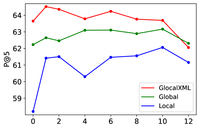
(a) EURLex-4K

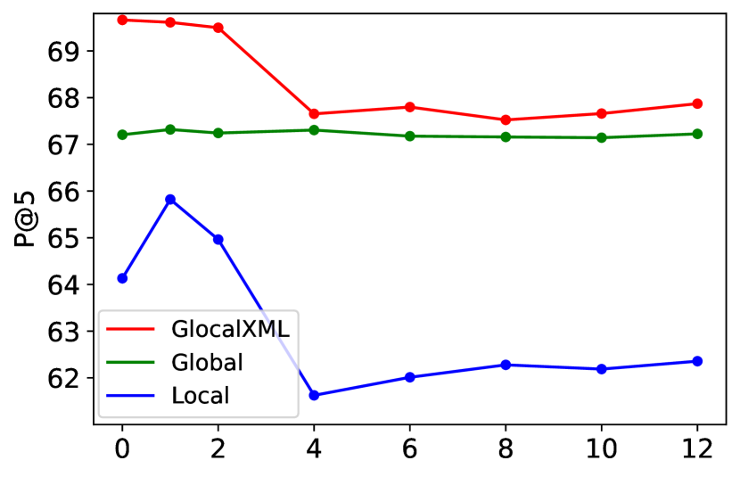
(b) Wiki10-31K

Figure 1: Ablation test on the effectiveness of combining the global feature ([CLS] embedding at the final layer) with different layers of local feature. The horizontal axis is the local layer number, the vertical axis is the P@5 performance. Layer $0$ corresponds to the original token embeddings.

4 Analysis on Local & Global Features

4.1 Single Model Performance

The performance of a single Roberta model is reported in table 3. The classifier with local feature inevitably underperforms that with the global feature, probably because the local classifier only shares a shallow Transformer backbone which is less expressive. Despite that, when the local and global features are combined, GlocalXML achieves the best performance, which could come from the complementary effect of local and global feature (analysed below).

4.2 Local Features on Different Layers

In figure 1, we show the performance of combining the global feature with different layers of local features. For efficiency considerations, we reduce the sequence length to $256$ for the experiments. The global feature uses the [CLS] embedding at the final layer of Roberta, while the local features are the token embeddings from Transformer layers $0-12$. The layer $0$ corresponds to the original token embedding without being passed to any Transformer block.

We observe that the performance of classification with the global feature is relatively stable which outperforms that with the local features. Our GlocalXML model with a combination of the two features achieves the best performance. For the Wiki10-31K dataset, GlocalXML achieves better performance when the features comes from layers $<3$, even with the original token embedding at layer $0$. The reason is that since this dataset has a large label space and each document has an average of $19$ labels, it is more difficult for the [CLS] embedding to summarize the text with distinctive word-level features peculiar to the labels. Therefore, the local classifier which allows labels to directly query for the keywords in the document could pick up the missing information. Combining the two leads to better results.

On both datasets, we observe that the performance of GlocalXML becomes worse when combined with the local features from higher layers, even if the local features from higher layers tend to perform better in EURLex-4K. The performance of GlocalXML is peaked when the local feature is at (near) layer $1$.

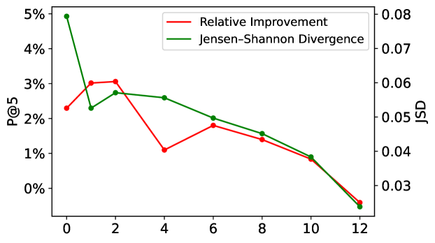
Figure 2: (EURLex-4K) the relative improvement of classification of GlocalXML over the global feature, and the JSD between predicted label distributions with global and local feature. We fix the global classifier and use the local feature from different layers.

Our hypothesis is: even if the token embedding at higher layer preserves the token meaning , it becomes more contextualized after multiple layers of self-attention. Consequently, querying from more contextualized embeddings makes the label harder to pick up the salient keywords information. In figure 2, we study the correlation between the relative improvement (red curve) of GlocalXML over the global classifier and the JSD (green curve) of the predicted label distributions by the local and global classifier. It reveals: 1) the distributions by local and global classifiers are more similar when a higher layer of word embeddings are used, and 2) a higher distribution similarity is correlated with a lower improvement of GlocalXML . This shows that querying from more contextualized word embeddings may degrade to querying the global embedding (as does the global classifier) and result in less information gain.

5 Conclusion

In this paper, we propose GlocalXML , a classification system integrating both the global and local features from the pre-trained Transformers. The global classifier uses [CLS] embedding as the summarization of document, and the local classifier uses the label-word attention to directly select salient part of texts for classification. Our model combines the two to capture different granularity of document semantics, which achieves superior or comparable performances over SOTA methods on the benchmark datasets.

References

- (1)
- Babbar and Schölkopf (2017) Rohit Babbar and Bernhard Schölkopf. 2017. Dismec: Distributed sparse machines for extreme multi-label classification. In Proceedings of the Tenth ACM International Conference on Web Search and Data Mining. 721–729.
- Chang et al. (2020) Wei-Cheng Chang, Hsiang-Fu Yu, Kai Zhong, Yiming Yang, and Inderjit S Dhillon. 2020. Taming pretrained transformers for extreme multi-label text classification. In Proceedings of the 26th ACM SIGKDD International Conference on Knowledge Discovery & Data Mining. 3163–3171.
- Devlin et al. (2018) Jacob Devlin, Ming-Wei Chang, Kenton Lee, and Kristina Toutanova. 2018. Bert: Pre-training of deep bidirectional transformers for language understanding. arXiv preprint arXiv:1810.04805 (2018).
- Jain et al. (2016) Himanshu Jain, Yashoteja Prabhu, and Manik Varma. 2016. Extreme multi-label loss functions for recommendation, tagging, ranking & other missing label applications. In Proceedings of the 22nd ACM SIGKDD International Conference on Knowledge Discovery and Data Mining. 935–944.
- Jiang et al. (2021) Ting Jiang, Deqing Wang, Leilei Sun, Huayi Yang, Zhengyang Zhao, and Fuzhen Zhuang. 2021. LightXML: Transformer with Dynamic Negative Sampling for High-Performance Extreme Multi-label Text Classification. arXiv preprint arXiv:2101.03305 (2021).
- Liu et al. (2017) Jingzhou Liu, Wei-Cheng Chang, Yuexin Wu, and Yiming Yang. 2017. Deep learning for extreme multi-label text classification. In Proceedings of the 40th International ACM SIGIR Conference on Research and Development in Information Retrieval. 115–124.
- Liu et al. (2019) Yinhan Liu, Myle Ott, Naman Goyal, Jingfei Du, Mandar Joshi, Danqi Chen, Omer Levy, Mike Lewis, Luke Zettlemoyer, and Veselin Stoyanov. 2019. Roberta: A robustly optimized bert pretraining approach. arXiv preprint arXiv:1907.11692 (2019).
- Loza Mencía and Fürnkranz (2008) Eneldo Loza Mencía and Johannes Fürnkranz. 2008. Efficient Pairwise Multilabel Classification for Large-Scale Problems in the Legal Domain. In Machine Learning and Knowledge Discovery in Databases, Walter Daelemans, Bart Goethals, and Katharina Morik (Eds.). Springer Berlin Heidelberg.
- McAuley and Leskovec (2013) Julian McAuley and Jure Leskovec. 2013. Hidden Factors and Hidden Topics: Understanding Rating Dimensions with Review Text. Association for Computing Machinery, 165–172. https://doi.org/10.1145/2507157.2507163
- Prabhu et al. (2018) Yashoteja Prabhu, Anil Kag, Shrutendra Harsola, Rahul Agrawal, and Manik Varma. 2018. Parabel: Partitioned label trees for extreme classification with application to dynamic search advertising. In Proceedings of the 2018 World Wide Web Conference. 993–1002.
- Wydmuch et al. (2018) Marek Wydmuch, Kalina Jasinska, Mikhail Kuznetsov, Róbert Busa-Fekete, and Krzysztof Dembczynski. 2018. A no-regret generalization of hierarchical softmax to extreme multi-label classification. Advances in neural information processing systems 31 (2018).
- Yang et al. (2019) Zhilin Yang, Zihang Dai, Yiming Yang, Jaime Carbonell, Ruslan Salakhutdinov, and Quoc V Le. 2019. Xlnet: Generalized autoregressive pretraining for language understanding. arXiv preprint arXiv:1906.08237 (2019).
- Ye et al. (2020) Hui Ye, Zhiyu Chen, Da-Han Wang, and Brian Davison. 2020. Pretrained Generalized Autoregressive Model with Adaptive Probabilistic Label Clusters for Extreme Multi-label Text Classification. In International Conference on Machine Learning. PMLR, 10809–10819.
- You et al. (2018) Ronghui You, Zihan Zhang, Ziye Wang, Suyang Dai, Hiroshi Mamitsuka, and Shanfeng Zhu. 2018. Attentionxml: Label tree-based attention-aware deep model for high-performance extreme multi-label text classification. arXiv preprint arXiv:1811.01727 (2018).
- Zubiaga (2012) Arkaitz Zubiaga. 2012. Enhancing Navigation on Wikipedia with Social Tags. arXiv:1202.5469 [cs.IR]