Cosmological Inflation in $f(Q,T)$ Gravity

Abstract

We study the cosmological inflation within the context of $f(Q,T)$ gravity, wherein $Q$ is the nonmetricity scalar and $T$ is the trace of the matter energy-momentum tensor. By choosing a linear combination of $Q$ and $T$, we first analyze the realization of an inflationary scenario driven via the geometrical effects of the linear $f(Q,T)$ gravity and then, we obtain the modified slow-roll parameters, the scalar and the tensor spectral indices, and the tensor-to-scalar ratio for the proposed model. In addition, by choosing three inflationary potentials, i.e. the power-law, hyperbolic and natural potentials, and by applying the slow-roll approximations, we calculate these inflationary observables in the presence of an inflaton scalar field. The results indicate that by properly restricting the free parameters, the proposed model provides appropriate predictions that are consistent with the observational data obtained from the Planck 2018. Also, we specify that the contribution of linear model of $f(Q,T)$ gravity with the hyperbolic and natural potentials can impose different restrictions on the parameters of these potentials. Furthermore, the predictions of natural inflation in this model are in good agreement with the joint Planck, BK15 and BAO data, justifying the use of the $f(Q,T)$ gravity.

I Introduction

In recent decades, a wide range of theoretical and observational studies have been conducted to describe the dynamics of the Universe, and the results appear to be almost in good agreement with the standard cosmological model, i.e., the $\Lambda$CDM model, which stems from general relativity (GR) Ferreira:2019xrr . On the other hand, the observations related to the cosmic microwave background radiation (CMB) through various surveys contain very important information about the formation and evolution of the Universe WMAP:2003elm ; WMAP:2006bqn ; WMAP:2008lyn ; Hinshaw2013 ; Planck:2018jri ; Planck:2018vyg . However, some challenging concepts, such as flatness and horizon problems, remain undesirable within the framework of the standard cosmological model Coley:2019yov . To solve such problems, it has been proposed to consider an epoch of accelerated expansion in the earliest stage of the evolution of the Universe, known as cosmic inflation Starobinsky1980 ; guth1981 ; lidd1982 ; Albrecht1982 .

The most appropriate way to explain the inflationary framework is to consider a scalar field known as inflaton, which is managed by a specific potential. In particular, the quantum fluctuations of the inflaton can give rise to an inflationary era and explain the origin of the large-scale structures. In other words, the cosmic inflation yields density perturbations, the impact of which can be observed in the measurement of CMB temperature anisotropies 2dFGRS:2001csf ; WMAP:2003syu ; SDSS:2003tbn ; SDSS:2003eyi . Moreover, to produce a long enough inflationary era, it is essential to impose the (so-called) slow-roll conditions on the inflaton field, under which the kinetic term of the inflaton field can usually be ignored. On the other hand, a wide range of potentials, that can be capable of describing an inflationary era, have carefully been investigated and constrained via the measurements of CMB anisotropies Hossain:2014coa ; Martin:2013nzq ; Geng:2015fla ; Martin:2015dha ; Huang:2015cke .

On the other side, although GR has so far provided the most accurate predictions for describing cosmological phenomena Will:2005va , it is undesirable to justify the dark sector (i.e., dark matter and dark energy) that its effects on the dynamics of the Universe is well consistent with the observational data Ishak2019 . The need to overcome such shortcomings motivated the investigation of alternative theories of gravity, see Refs. Farhoudi2006 ; Felice ; Sotiriou2010 ; Nojiri2011 ; capozziello2011 ; clifton ; Farajollahi2012 ; Shabani2014 ; Joyce2015 ; Bueno2016 ; zare1 ; khosravi2016 ; Nojiri:2017ncd ; quiros2019 ; Mishra2020 and references therein. In this regard, various modified theories of gravity have also been considered for inflationary cosmology in the hope that their predictions can better justify the observational data Myrzakulov:2015qaa ; DeLaurentis:2015fea ; Sebastiani:2016ras ; Tirandari:2017nzy ; saba ; RSFM ; Chakraborty:2018scm ; Bernardo ; Kausar2019 ; Bhattacharjee:2020jsf ; Jalalzadel-et-al ; Gamonal:2020itt ; TQ.Do ; baffou ; faraji ; Bhattacharjee ; Chen:2022dyq ; Zhang:2021ppy .

Another approach to structuring a more general theory than GR is to consider geometry beyond the Riemannian one. The first study in this area was carried out by Weyl to achieve a geometric interpretation for electromagnetism and a unified theory for gravitation and electromagnetism Weyl1918 ; Weyl1919 ; Wheeler2018 . He assumed that under the parallel transformation of a vector, in addition to the direction of the vector, its length also changes. In this generalization of geometry, Weyl introduced a compensating vector field. In this idea, the connection of the system can be decomposed into two connections. One of those connections describes the vector length, and the other one, a Levi-Civita connection, expresses the vector direction under the parallel transportation. Both of these connections are torsionless within the framework of the Weyl geometry. Weyl tried to interpret the introduced vector field as the electromagnetic potential, however his theory was not successful and even was rejected by himself Weyl1921 .

However, Dirac tried to revive the Weyl geometry. Indeed, he showed Dirac that the difference between the Weyl geometry and the Riemannian one is in the expression of the partial derivative. In other words, under the Weyl gauge transformation, the Weyl space is reduced to a Riemannian one with a metric that is conformally related to the original metric. Nevertheless, it has been claimed Hayashi that the Weyl theory cannot describe the electromagnetic interaction because the vector field introduced by Weyl does not couple to the spinor, unlike the electromagnetic potential. Although the success of the Weyl theory was rather limited from the physical point of view, it presented some interesting points. Indeed, one of the most important features of the Weyl geometry is providing the nonzero covariant derivative of the metric tensor, which geometrically led to a quantitative definition called nonmetricity.

In order to achieve a simpler geometrical formalism for gravity, the teleparallel equivalent of GR was proposed that uses the Weitzenböck connection with zero curvature and nonmetricity tensors but nonzero torsion weiz ; TEGR .

Another formalism, known as the symmetric teleparallel gravity, has been constructed using a connection with zero curvature and torsion tensors but with a nonmetricity tensor describing gravitational interactions STG . The symmetric teleparallel gravity was modified Jimenez2018 into the coincident GR and $f(Q)$ gravity, which achieves a specific class with a vanishing connection in the so-called coincident gauge. One of the most important points of this theory is that it deprives gravity of any inertial character and separates inertial and gravitational effects, which cannot be done in GR telepalatini . The symmetric teleparallel gravity provides another geometrical description of gravitation that is dynamically equivalent to GR. This theory is described by the Einstein-Hilbert action in the absence of boundary terms. Its construction naturally leads to self-accelerating cosmological solutions in the early and late-time Universe. The cosmological and astrophysical aspects of this theory have been investigated in Refs. Jimenez2018 ; Harko2018 ; Lu2019 ; BeltranJimenez:2019tme ; DAmbrosio:2021pnd ; DAmbrosio:2021zpm ; Narawade .

Another proposed theory as an alternative to GR is $f(Q,T)$ gravity Xu:2019sbp , wherein the gravitational action is determined by an arbitrary function of the nonmetricity scalar, $Q$, and the trace of the energy-momentum tensor, $T$. This theory is in fact an extension of the symmetric teleparallel gravity and $f(Q)$ gravity Jimenez2018 ; Harko2018 . Till now, some cosmological aspects of $f(Q,T)$ gravity have been studied, e.g., observational constraints of $f(Q,T)$ gravity Arora:2020tuk , cosmological implications of its Weyl-type gravity Xu:2020yeg ; Gadbail:2021kgd ; Gadbail:2021fjf , energy conditions in $f(Q,T)$ gravity Arora:2020iva ; Arora:2021jik ; Arora:2020met , Friedmann-Lemaître-Robertson-Walker (FLRW) cosmology in $f(Q,T)$ gravity Godani:2021mld , transit cosmological models of $f(Q,T)$ gravity Pradhan2021 , and dynamical aspects and cosmic acceleration in $f(Q,T)$ gravity Pati:2021ach ; Agrawal:2021rur ; 2022Arora ; Pati:2021zew . Also, a further extension of $f(Q,T)$ gravity has been performed to squared symmetric teleparallel gravity $f(Q,T_{\mu\nu}T^{\mu\nu})$ Rudra .

In this work, we intend to investigate the cosmological inflation within the context of linear $f(Q,T)$ gravity. In this respect, the outline of the work is as follows. In Sec. II, we concisely introduce the context of cosmological inflation. Then, in Sec. III, we briefly review the theoretical framework of $f(Q,T)$ gravity. Accordingly, in Sec. IV, we calculate the cosmological inflation within the context of such a gravity and hereupon, discuss the relevant results. Moreover, in Sec. V, we calculate the cosmological inflation for a linear functional form of $f(Q,T)$ gravity in the presence of a scalar field, and then, specify inflationary observables by considering three different inflationary potentials. Finally, in Sec. VI, we scrutinize the results and summarize the findings. Also, we provide an overview of some prerequisites related to the $f(Q,T)$ gravity in an appendix.

II Cosmological Inflation

The simplest model of inflation is based on GR and an isotropic and homogeneous scalar field called the inflaton. The dynamics of such an inflaton field can be defined via the action

$$S=\int\sqrt{-g}\left(\dfrac{R}{2\kappa}+L_{\rm m}^{[\phi]}\right){\rm d}^{4}x,$$ (1)

where $g$ is the determinant of the metric, $R$ is the Ricci scalar, $\kappa=8\pi=1/{\rm M^{2}_{Pl}}$ (in the natural units $\hbar=1=c$ and $G=1$) and the lower case Greek indices run from zero to three. Also, $L_{\rm m}^{[\phi]}$ is the Lagrangian of the inflaton field defined as

$$L_{\rm m}^{[\phi]}=-\dfrac{1}{2}g^{\mu\nu}\partial_{\mu}\phi\partial_{\nu}\phi-V(\phi),$$ (2)

where $\phi\equiv\phi(t)$ is the scalar field and $V(\phi)$ is the potential of the scalar field that depends on one or more free parameters lythandriotto . During the inflationary era, the inflaton slowly rolls down along its relatively flat potential.

The variation of action (1) with respect to the metric gives

$$R_{\mu\nu}-\dfrac{1}{2}Rg_{\mu\nu}=\kappa T_{\mu\nu},$$ (3)

where $T_{\mu\nu}$ is the energy-momentum tensor that, generally, defined as

$$T_{\mu\nu}\equiv-\dfrac{2}{\sqrt{-g}}\frac{\delta(\sqrt{-g}L_{\rm m})}{\delta g^{\mu\nu}}=g_{\mu\nu}L_{\rm m}-2\dfrac{\partial L_{\rm m}}{\partial g^{\mu\nu}}.$$ (4)

By substituting relation (2) into relation (4), it gives

$$T_{\mu\nu}^{[\phi]}=\partial_{\mu}\phi\partial_{\nu}\phi-g_{\mu\nu}\left[\dfrac{1}{2}\partial_{\sigma}\phi\partial^{\sigma}\phi+V(\phi)\right].$$ (5)

We also assume the spatially flat FLRW spacetime

$$ds^{2}=-dt^{2}+a^{2}(t)(dx^{2}+dy^{2}+dz^{2}),$$ (6)

where $a(t)$ is the cosmological scale factor as a function of the cosmic time $t$ with the present time Universe $t_{0}$ as $a(t_{0})=1$. The energy-momentum tensor of the inflaton field can be declared as a perfect fluid with a linear barotropic equation of state as $p^{[\phi]}=w\rho^{[\phi]}$, in which the energy density, $\rho^{[\phi]}$, and the pressure density, $p^{[\phi]}$, are

$$\rho^{[\phi]}=\dfrac{1}{2}\dot{\phi}^{2}+V(\phi)\qquad{\rm and}\qquad p^{[\phi]}=\dfrac{1}{2}\dot{\phi}^{2}-V(\phi),$$ (7)

where dot represents the derivative with respect to the cosmic time. The dimensionless related parameter of the equation of state also is

$$w^{[\phi]}=\dfrac{p^{[\phi]}}{\rho^{[\phi]}}=\dfrac{\dot{\phi}^{2}-2V}{\dot{\phi}^{2}+2V}.$$ (8)

Now, under these considerations and by using Eqs. (3), (5), (6) and (7), we easily obtain the Friedmann equations as

$$H^{2}=\dfrac{\kappa}{3}\left[\dfrac{\dot{\phi}^{2}}{2}+V(\phi)\right],$$ (9)

$$H^{2}+\dot{H}=-\dfrac{\kappa}{3}\left[\dot{\phi}^{2}-V(\phi)\right],$$ (10)

$$\dot{H}=-\dfrac{\kappa}{2}\dot{\phi}^{2},$$ (11)

where $H(t)\equiv\dot{a}/a$ is the Hubble parameter. To achieve the time evolution of the scalar field, by taking the time derivative of Eq. (9) and substituting Eq. (11) into the resulted relation, we obtain the Klein-Gordon equation as

$$\ddot{\phi}+3H\dot{\phi}+V^{\prime}=0,$$ (12)

where the prime denotes derivative with respect to the scalar field.

Inflation is an accelerated expansion era in the early Universe, wherein the comoving Hubble horizon shrinks in time, i.e.,

$$\dfrac{d(aH)^{-1}}{dt}=-\dfrac{\ddot{a}}{\dot{a}^{2}}=-\dfrac{1}{a}\left(1-\epsilon_{1}\right)<0.$$ (13)

In this relation, $\epsilon_{1}<1$ is the first slow-roll parameter, which is defined as liddle1994 ; mokhanov

$${\rm\epsilon_{1}}(t)\equiv-\dfrac{\dot{H}}{H^{2}}.$$ (14)

Moreover, there are several possible sets of such slow-roll parameters that are useful to define in terms of the e-folding number, $N$, namely ency

$${\rm\epsilon_{n+1}}(t)\equiv\dfrac{\rm{d\ln|\epsilon_{n}(t)|}}{\rm{dN}},$$ (15)

where $n\geq 0$ is an integer and ${\rm\epsilon_{0}}(t)\equiv H_{\rm end}/H$. This relation is known as the Hubble flow parameters or the Hubble slow-roll parameters. The e-folding number somehow describes the rate of the expansion of inflation as a natural logarithm of the scale factor intcosminf ; tasi lec

$$N\equiv\ln(\dfrac{a_{\rm end}}{a})=\int_{t}^{t_{\rm end}}H\rm{dt},$$ (16)

where the index ‘${\rm end}$’ denotes the value of quantities at the end of inflation. From definition (15), the second slow-roll parameter is

$${\rm\epsilon_{2}}=\dfrac{\dot{{\rm\epsilon_{1}}}}{H{\rm\epsilon_{1}}}=\dfrac{\ddot{H}}{\dot{H}H}-2\dfrac{\dot{H}}{H^{2}}.$$ (17)

It is known ency that if the condition $|{\rm\epsilon_{n}}|\ll 1$ is met, inflation will occur and will continue long enough to solve the standard cosmological problems. Also, inflation ends when the first slow-roll parameter reaches the unit, i.e., ${\rm\epsilon_{1}}=1$.

Potential Representation of Slow-Roll Parameters

As mentioned, an inflationary scenario at the early stages of the formation of the Universe can be described by the slow-roll conditions. Hence, calculating the slow-roll parameters while satisfying the slow-roll conditions can be considered as the first step in inflationary calculations. These parameters can also be written in terms of the inflationary potential used.

By substituting Eqs. (9) and (11) into definition (14), one obtains the first slow-roll parameter, usually denoted by $\epsilon$, in terms of scalar field as

$${\rm\epsilon}\equiv\epsilon_{1}=\dfrac{3}{2}\dfrac{\dot{\phi}^{2}}{\dfrac{\dot{\phi}^{2}}{2}+V}.$$ (18)

As a result, satisfying $\epsilon\ll 1$ leads to

$$\dot{\phi}^{2}\ll|V|.$$ (19)

By applying the above condition to relation (18), $\epsilon$ can be approximated as

$$\epsilon\approx\dfrac{3}{2}\dfrac{\dot{\phi}^{2}}{|V|}.$$ (20)

Similar to the first slow-roll parameter, the usual second slow-roll parameter can also be defined as

$$\eta\equiv 2\epsilon-\dfrac{\epsilon_{2}}{2}=-\dfrac{\dot{H}}{H^{2}}-\dfrac{\ddot{H}}{2H\dot{H}}\approx-\dfrac{|\ddot{\phi}|}{H|\dot{\phi}|},$$ (21)

where, in the last approximation, relation (19) and Eqs. (9)-(11) have been used. Furthermore, the condition $|\eta|\ll 1$ yields

$$|\ddot{\phi}|\ll H|\dot{\phi}|,$$ (22)

which, together with condition (19), are known as the slow-roll conditions. The slow-roll conditions manage the dynamics of inflationary scenarios in such a way that it will lead to inflation if these conditions can be fulfilled, and when those are violated, inflation will end. Accordingly, by using the slow-roll conditions, Eqs. (9) and (12) can also be approximated to

$$H^{2}\approx\dfrac{\kappa}{3}V(\phi),$$ (23)

$$\dot{\phi}\approx-\dfrac{V^{\prime}}{3H}.$$ (24)

Now, via Eqs. (23) and (24), the slow-roll parameters can be written in terms of the inflationary potential and its derivatives as

$$\epsilon\approx\dfrac{1}{2\kappa}\left(\dfrac{V^{\prime}}{V}\right)^{2},$$ (25)

and liddle1994 ; weinberg ; myrzak

$$\eta\approx\dfrac{1}{\kappa}\dfrac{V^{\prime\prime}}{V}.$$ (26)

Relations (25) and (26) are known as the potential slow-roll parameters, which are distinct from the Hubble slow-roll parameters. Using the slow-roll approximations and the equation of state as $w^{[\phi]}\approx-1$, the e-folding number, relation (16), can be calculated in terms of the inflationary potential as

$$N=\int_{\phi}^{\phi_{\rm end}}\dfrac{H}{\dot{\phi}}{\rm d}\phi=\kappa\int_{\phi_{\rm end}}^{\phi}\dfrac{V}{V^{\prime}}{\rm d}\phi.$$ (27)

Up to now, we have introduced the slow-roll parameters in both Hubble and potential representations within the context of the cosmological inflation scenario. In the following, we will briefly review the theoretical framework of $f(Q,T)$ gravity and its cosmological implications.

III The Framework of $f(Q,T)$ Gravity

To avoid any digressions, we review some prerequisites related to the $f(Q,T)$ gravity in an appendix.

Following Ref. Xu:2019sbp , we consider the $f(Q,T)$ gravity action

$$S=\int\sqrt{-g}\left[\dfrac{f(Q,T)}{2\kappa}+L_{\rm m}\right]{\rm d}^{4}x,$$ (28)

where in addition to the metric, this action also varies with respect to the connection, which is assumed to be torsionless with a zero Riemann tensor, while accepting nonmetricity.

The variation of action (28) with respect to the metric leads to the modified field equations

$$\begin{array}[]{l}\kappa\,T_{\mu\nu}=-\dfrac{2}{\sqrt{-g}}\bigtriangledown_{\alpha}\left(f_{Q}\sqrt{-g}P^{\alpha}{}_{\mu\nu}\right)-\dfrac{f\,g_{\mu\nu}}{2}\\ \\ \kern 16.79993pt+f_{T}\left(T_{\mu\nu}+\Theta_{\mu\nu}\right)-f_{Q}\left(P_{\mu\alpha\beta}Q_{\nu}{}^{\alpha\beta}-2Q^{\alpha\beta}{}_{\mu}P_{\alpha\beta\nu}\right),\end{array}$$ (29)

where

$$\Theta_{\mu\nu}\equiv g^{\alpha\beta}\dfrac{\delta T_{\alpha\beta}}{\delta g^{\mu\nu}},~{}~{}f_{Q}\equiv\dfrac{\partial f(Q,T)}{\partial Q},~{}~{}f_{T}\equiv\dfrac{\partial f(Q,T)}{\partial T}.$$ (30)

Furthermore, $P^{\alpha}{}_{\mu\nu}$ is the superpotential of the model, which is defined as

$$P^{\alpha}{}_{\mu\nu}\equiv-\dfrac{1}{2}L^{\alpha}{}_{\mu\nu}+\dfrac{1}{4}\left(Q^{\alpha}-\tilde{Q}^{\alpha}\right)g_{\mu\nu}-\dfrac{1}{4}\delta^{\alpha}_{(\mu}Q_{\nu)}.$$ (31)

In this relation, each of ${Q}^{\alpha}$ and $\tilde{Q}^{\alpha}$ is the trace of the nonmetricity tensor defined as

$${Q}_{\alpha}\equiv Q_{\alpha}{}^{\mu}{}_{\mu}\qquad{\rm and}\qquad\tilde{Q}_{\alpha}\equiv Q^{\mu}{}_{\alpha\mu}.$$ (32)

The variation of action (28) with respect to the connection can be performed while imposing two constraints $R^{\alpha}{}_{\beta\mu\nu}=0$ and $\tau^{\alpha}{}_{\mu\nu}=0$, and using the Lagrange multiplier method. Consequently the corresponding field equations are

$$\bigtriangledown_{\mu}\bigtriangledown_{\nu}$2\sqrt{-g}f_{Q}P^{\mu\nu}{}_{\alpha}+\kappa\,H_{\alpha}{}^{\mu\nu}$=0,$$ (33)

where $H_{\alpha}{}^{\mu\nu}$ is the hyper-momentum tensor density defined as

$$H_{\alpha}{}^{\mu\nu}\equiv\dfrac{f_{T}\sqrt{-g}}{2\kappa}\dfrac{\delta\,T}{\delta\Gamma^{\alpha}{}_{\mu\nu}}+\dfrac{\delta$\sqrt{-g}\,{\rm L_{m}}$}{\delta\Gamma^{\alpha}{}_{\mu\nu}}.$$ (34)

We also assume the spatially flat FLRW spacetime, metric (6), and consider the energy-momentum tensor as a perfect fluid, i.e.,

$$T_{\mu\nu}=\left(\rho+p\right)u_{\mu}u_{\nu}+p\,g_{\mu\nu},$$ (35)

where $\rho$, $p$ and $u^{\mu}$ are the energy density, the pressure density, and the four-vector velocity of the perfect fluid, respectively. In an adapted coordinate system, i.e. the Cartesian coordinates in the spatial variables of the line-element (6) in which the connection is zero (the coincident gauge), one obtains the nonmetricity scalar to be $Q=6H^{2}$. Hence the modified Friedmann equations are

$$\kappa\,\rho=\dfrac{f}{2}-6FH^{2}-\dfrac{2\tilde{G}}{1+\tilde{G}}\left(\dot{F}H+F\dot{H}\right),$$ (36)

$$\kappa\,p=-\dfrac{f}{2}+6FH^{2}+2\left(\dot{F}H+F\dot{H}\right),$$ (37)

where $F\equiv f_{Q}$ and $\kappa\tilde{G}\equiv f_{T}$ have been defined for simplicity. Under these situations, one obtains the evolution of the Hubble parameter as

$$\dot{H}+\dfrac{\dot{F}}{F}H=\dfrac{\kappa}{2F}\left(1+\tilde{G}\right)\left(\rho+p\right),$$ (38)

where $F\neq 0$ has been assumed. By introducing the effective pressure and energy densities, one can rewrite the modified Friedmann equations as

$$3H^{2}=\kappa\rho^{[\rm eff]}=\dfrac{f}{4F}-\dfrac{\kappa}{2F}\left[\left(1+\tilde{G}\right)\rho+\tilde{G}p\right],$$ (39)

$$2\dot{H}+3H^{2}=-\kappa p^{[\rm eff]}=\dfrac{f}{4F}-\dfrac{2\dot{F}H}{F}$$

$$~{}~{}~{}~{}~{}~{}~{}~{}~{}~{}~{}~{}~{}~{}~{}~{}~{}+\dfrac{\kappa}{2F}\left[\left(1+\tilde{G}\right)\rho+\left(2+\tilde{G}\right)p\right].$$ (40)

Also, taking the time derivative of Eq. (39) while using Eqs. (39) and (40) yields the convenient continuity equation

$$\dot{\rho}^{[\rm eff]}+3H\left(\rho^{[\rm eff]}+p^{[\rm eff]}\right)=0.$$ (41)

Moreover, by substituting Eq. (38) into Eq. (36) while using the linear barotropic equation of state, we obtain the evolution of energy density to be

$$\rho=\dfrac{f-12H^{2}F}{2\kappa\left[(1+w)\tilde{G}+1\right]}.$$ (42)

IV Modeling an Inflationary Scenario in $f(Q,T)$ Gravity

Inflation can be realized by a scalar field called inflaton or from modification of gravity. In this section, we analyze the slow-roll inflation within the framework of a special model of the $f(Q,T)$ gravity. That is, we consider a linear functional form of $f(Q,T)$ gravity, i.e. $f(Q,T)=\alpha\,Q+\beta\,T$, with $\alpha=F\neq 0$ and $\beta$ as free constant parameters of the model. The model obviously reduces to $f(Q)$ gravity for $\beta=0$ that has been considered in, e.g., Ref. Hassan2021 , and the cosmological evolution of $f(Q,T)$ gravity has been studied in Ref. Xu:2019sbp .

By taking a linear barotropic equation of state and $T=-\rho+3p$, Eqs. (38), (39), (40) and (42) reduce to

$$\dot{H}=\dfrac{\left(\kappa+\beta\right)\rho\left(1+w\right)}{2\alpha},$$ (43)

$$3H^{2}=\kappa\rho^{[\rm eff]}=\dfrac{\left[(w-3)\beta-2\kappa\right]\rho}{2\alpha},$$ (44)

$$2\dot{H}+3H^{2}=-\kappa p^{[{\rm eff}]}=\dfrac{\rho\left[\left(3w-1\right)\beta+2w\kappa\right]}{2\alpha},$$ (45)

$$\rho=\dfrac{-6\alpha H^{2}}{\beta\left(3-w\right)+2\kappa},$$ (46)

where

$$(1+w)\beta+\kappa\neq 0\qquad{\rm and}\qquad(w-3)\beta-2\kappa\neq 0$$ (47)

have been assumed. In addition, in the case of $\beta=-\kappa$ and/or $w=-1$, Eq. (43) gives $\dot{H}=0$, and hence $H$ (and in turn, $\rho$) is constant. These cases lead either to a de Sitter expansion for nonzero $H$ or to the Minkowski metric for $H=0$. Therefore, we also exclude these values in the numerical calculations of inflationary observables.

Note that, contrary to what has been claimed in Ref. Xu:2019sbp , no consistency condition for the parameter $\beta$ can be obtained from Eqs. (43), (44) and (45). Hence, the evolution of the linear model of $f(Q,T)$ gravity is not fixed on a de Sitter expansion.

In continuation, Eqs. (44) and (45) lead to an effective parameter of the equation of state for this model as

$$w^{[{\rm eff}]}=\dfrac{p^{[{\rm eff}]}}{\rho^{[{\rm eff}]}}=-1-\dfrac{2\left(\kappa+\beta\right)\left(1+w\right)}{\left(w-3\right)\beta-2\kappa}.$$ (48)

In this situation, different conditions can be considered as follows.

• The effective de Sitter accelerated expansion (i.e., $w^{[{\rm eff}]}=\,-1$) will be realized if one has either ($w=-1$ with $\beta\neq-\kappa/2$) or ($\beta=-\kappa$ with $w\neq 1$). However, we have already excluded $\beta=-\kappa$ and $w=-1$ values.

• The effective phantom accelerated phase (i.e., $w^{[{\rm eff}]}<-1$) will occur if one has ($\beta=0$ with $w<-1$), or ($\beta>0$ with either $w<-1$ or $w>3+2\kappa/\beta$), or ($\beta<-\kappa$ with either $w<-1$ or $w>3+2\kappa/\beta$), or ($-\kappa<\beta<-\kappa/2$ with $-1<w<3+2\kappa/\beta$), or ($-\kappa/2<\beta<0$ with $3+2\kappa/\beta<w<-1$).

• The effective quintessence accelerated evolution (i.e., $-1<w^{[{\rm eff}]}<-1/3$) will happen if one has ($\beta=0$ with $-1<w<-1/3$, as expected), or ($w=0$ with $\beta<-\kappa$), or ($\beta<-\kappa$ with $-1<w<-\kappa/(3\kappa+4\beta)$ [note that, this value includes $w=0$ and for $\beta\rightarrow-\kappa$, its upper limit is $w<1$]), or ($-\kappa<\beta<-3\kappa/4$ with either $w>-\kappa/(3\kappa+4\beta)$ or $w<-1$), or ($\beta=-3\kappa/4$ with $w<-1$), or ($-3\kappa/4<\beta<-2\kappa/3$ with $-\kappa/(3\kappa+4\beta)<w<-1)$), or ($\beta=-2\kappa/3$ with $-3<w<-1$), or ($-2\kappa/3<\beta<-\kappa/2$ with $-\kappa/(3\kappa+4\beta)<w<-1$), or ($-\kappa/2<\beta<0$ with $-1<w<-\kappa/(3\kappa+4\beta)$), or ($\beta>0$ with $-1<w<-\kappa/(3\kappa+4\beta)$).

On the other hand, by substituting Eq. (46) into Eq. (43) the following differential equation can be obtained

$$\dot{H}-3A(w,\beta)H^{2}=0,$$ (49)

where

$$A(w,\beta)\equiv\dfrac{\left(w+1\right)\left(\kappa+\beta\right)}{\left(w-3\right)\beta-2\kappa}.$$ (50)

Eq. (49) is a differential equation for the Hubble parameter that gives

$$H=\dfrac{\beta\left(w-3\right)-2\kappa}{\beta\left[w\left(-3t+C\right)-3t-3C\right]-\kappa\left(3tw+3t+2C\right)},$$ (51)

where $C$ is an integration constant. However, the time derivatives of the Hubble parameter can also be extracted from the above relation as

$$\dot{H}\!=\!\dfrac{3\left(w+1\right)\left(\kappa+\beta\right)\left[\beta\left(w-3\right)-2\kappa\right]}{\big{\{}\beta\left[w\left(-3t+C\right)-3t-3C\right]-\kappa\left(3tw+3t+2C\right)\!\big{\}}^{2}},$$ (52)

$$\ddot{H}\!=\!\dfrac{18\left(w+1\right)^{2}\left(\kappa+\beta\right)^{2}\left[\beta\left(w-3\right)-2\kappa\right]}{\big{\{}\beta\left[w\left(-3t+C\right)-3t-3C\right]-\kappa\left(3tw+3t+2C\right)\!\big{\}}^{3}}.$$ (53)

The main purpose of gravitational theories in properly describing cosmological inflation is to provide consistent predictions with the observational data. For this purpose, one has to examine the theoretical predictions of the proposed gravitational models for the inflationary observables that are as follows ency ; liddlebook ; higer ; Lythandliddle .

• The scalar spectral index:

  $$n_{\rm S}=1+\dfrac{{\rm d}\ln(\Delta_{\rm S}^{2})}{{\rm d}\ln{\rm k}}=1-6\epsilon+2\eta.$$ (54)

• The tensor spectral index:

  $$n_{\rm T}=\dfrac{{\rm d}\ln(\Delta_{\rm T}^{2})}{{\rm d}\ln{\rm k}}=-2\epsilon.$$ (55)

• The tensor-to-scalar ratio:

  $$r=\dfrac{\Delta_{\rm T}^{2}({\rm k})}{\Delta_{\rm S}^{2}({\rm k})}=16\epsilon.$$ (56)

In relations (54), (55) and (56), $\Delta_{\rm S}$ and $\Delta_{\rm T}$ are respectively the dimensionless power spectrum for scalar perturbations and tensor perturbations, and ${\rm k}=aH$. By substituting Eqs. (51), (52) and (53) into Eqs. (14), (17) and (21), the slow-roll parameters for the proposed gravitational model are

$${\rm\epsilon}=\dfrac{-3\left(w+1\right)\left(\kappa+\beta\right)}{\beta\left(w-3\right)-2\kappa},\quad{\rm\epsilon_{2}}=0\quad{\rm and}\quad\eta=2\epsilon.$$ (57)

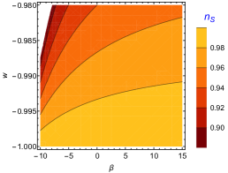
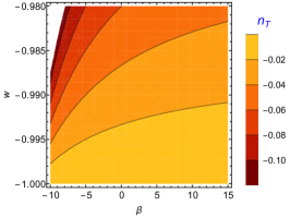
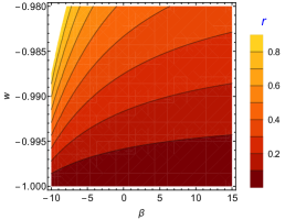
Figure 1: [color online] Inflationary observables as functions of the dimensionless parameter of the equation of state $w$ and the free parameter $\beta$, wherein (a) shows the scalar spectral index, $n_{\rm S}$, (b) indicates the tensor spectral index, $n_{\rm T}$, and (c) demonstrates the tensor-to-scalar ratio, $r$.

Table 1: Inflationary observables for different values of $w$ and $\beta$.

$w$	$\beta$	$n_{\rm S}$	$r$	$n_{\rm T}$
-0.984	14.1	0.96461	0.28305	-0.03538
-0.986	5.4	0.96427	0.28578	-0.03572
-0.988	0.3	0.96441	0.28466	-0.03558
-0.990	-3.5	0.96423	0.28608	-0.03576
-0.992	-6.2	0.96437	0.28502	-0.03562
-0.994	-8.3	0.96456	0.28345	-0.03543
-0.996	-0.29	0.98785	0.09713	-0.01214
-0.998	-8.5	0.98773	0.09814	-0.01226

Now, let us calculate the inflationary observables in the $f(Q,T)=\alpha\,Q+\beta\,T$ gravity and compare the results with the observational data. In this regard, the latest constraints from the Planck collaboration on the scalar spectral index and the tensor-to-scalar ratio are Planck:2018jri

$$n_{\rm S}=0.9649\pm 0.0042\quad{\rm at}\ 68\%\,{\rm CL},$$ (58)

(59)

$$r<0.10\quad{\rm at}\ 95\%\,{\rm CL}.$$ (60)

However, by the joint Planck, BK15 and BAO data, further constraint tightened the upper limit on r to be

$$r<0.056\quad{\rm at}\ 95\%\,{\rm CL}.$$ (61)

On the other hand, using the slow-roll parameters, according to relations (54), (55) and (56) and (57), the inflationary observables for the proposed gravitational model are obtained to be

$$n_{\rm S}=\dfrac{\left(7w+3\right)\beta+\left(4+6w\right)\kappa}{\beta\left(w-3\right)-2\kappa},$$ (62)

$$n_{\rm T}=\dfrac{6\left(w+1\right)\left(\kappa+\beta\right)}{\beta\left(w-3\right)-2\kappa},$$ (63)

$$r=\dfrac{-48\left(w+1\right)\left(\kappa+\beta\right)}{\beta\left(w-3\right)-2\kappa}.$$ (64)

As is clear from the above relations, the inflationary observables do not depend on the free parameter $\alpha$ and the e-folding number. Instead, the dependence of these observations is on the free parameter $\beta$ and the dimensionless parameter of the equation of state $w$.

In order to realize the robustness of the model in the case of cosmological inflation, the comparison of the free parameters of the model with the latest observational data have been investigated. The numerical results for the scalar spectral index, the tensor spectral index, and the tensor-to-scalar ratio as functions of $w$ and $\beta$ have been shown in Fig. 1 in the range of $[-1.000,-0.980]$ and $[-10,15]$, respectively. It can be inferred from the contour plots that the values of both $w$ and $\beta$ parameters affect on the values of the inflationary observables. Also, the consistent values of inflationary observables for some values of parameters $w$ and $\beta$ have been given in Table 1. As is clear, the theoretical predictions of the proposed gravitational model for some values of $w$ and $\beta$ for $n_{\rm S}$ and $r$ are in agreement with the observational data. However, for the values ($w=-1$ with $\beta\neq-\kappa/2$) and/or ($\beta=-\kappa$ with $w\neq 1$), one obtains a de Sitter expansion, which indicates that inflation does not occur (besides, $\rho$ is constant in these cases). In addition, for the values ($w=-1$ with $\beta=-\kappa/2$) and/or ($\beta=-\kappa$ with $w=1$), which do not satisfy the second condition (47), Eq. (44) implies $H=0$, and in turn $a(t)$ to be constant, and thus the solution to the field equations is the Minkowski metric with no inflation.

V Slow-Roll Inflation in $f(Q,T)$ Gravity with Scalar Field

In this section, we are going to analyze the cosmological inflation within the context of the linear $f(Q,T)$ gravity in the presence of a scalar field as the matter Lagrangian, i.e. relation (2), and as a perfect fluid with the associated linear barotropic equation of state that is just a function of the cosmic time. Hence by relation (5), the trace of the energy-momentum tensor is

$$T^{[\phi]}=\dot{\phi}^{2}-4V.$$ (65)

Also, by substituting relations (7) into Eqs. (39) and (40), we obtain the components of the effective energy-momentum tensor as

$$\rho^{[\rm eff]}=-\dfrac{\left(\kappa+\beta\right)\dot{\phi}^{2}+2\,V(\phi)\left(\kappa+2\beta\right)}{2\kappa\alpha},$$ (66)

$$p^{[\rm eff]}=-\dfrac{\left(\kappa+\beta\right)\dot{\phi}^{2}-2\,V(\phi)\left(\kappa+2\beta\right)}{2\kappa\alpha}.$$ (67)

Accordingly, the effective dimensionless parameter of the equation of state obviously is

$$w^{[\rm eff]}=\dfrac{\left(\kappa+\beta\right)\dot{\phi}^{2}-2\,V(\phi)\left(\kappa+2\beta\right)}{\left(\kappa+\beta\right)\dot{\phi}^{2}+2\,V(\phi)\left(\kappa+2\beta\right)}.$$ (68)

Moreover, by considering Eqs. (66) and (67), the modified Friedmann equations (39) and (40) can be translated into the formulas

$$\dfrac{3}{2}H^{2}=-\dfrac{\left(\kappa+\beta\right)\dot{\phi}^{2}+2\,V(\phi)\left(\kappa+2\beta\right)}{4\alpha},$$ (69)

$$2\dot{H}+\dfrac{3}{2}H^{2}=\dfrac{3\left(\kappa+\beta\right)\dot{\phi}^{2}-2\,V(\phi)\left(\kappa+2\beta\right)}{4\alpha}.$$ (70)

From these relations, $\dot{H}$ reads

$$\dot{H}=\dfrac{\dot{\phi}^{2}}{2\alpha}\left(\kappa+\beta\right),$$ (71)

therefore we exclude $\beta=-\kappa$ again. By taking the time derivative of Eq. (69) and substituting Eq. (71) into the result, we obtain the modified Klein-Gordon equation as

$$\ddot{\phi}\left(\kappa+\beta\right)+3H\dot{\phi}\left(\kappa+\beta\right)+V^{\prime}\left(\kappa+2\beta\right)=0.$$ (72)

Now, let us calculate the extended slow-roll parameters within the context of the linear $f(Q,T)$ gravity. For this purpose, one has to insert Eqs. (69) and (71) into Eq. (14). Accordingly, the first extended slow-roll parameter is obtained as

$${\rm\epsilon}=\dfrac{3\left(\kappa+\beta\right)\dot{\phi}^{2}}{\left(\kappa+\beta\right)\dot{\phi}^{2}+2\,V\left(\kappa+2\beta\right)}.$$ (73)

As inflation will occur if ${\rm\epsilon}\ll 1$, hence the slow-roll condition (19) within the context of the linear $f(Q,T)$ gravity in this situation will be modified as

$$\left(\kappa+\beta\right)\dot{\phi}^{2}\ll V\left(\kappa+2\beta\right).$$ (74)

By taking the time derivative of Eq. (71), one obtains

$$\ddot{H}=\dfrac{\dot{\phi}\ddot{\phi}}{\alpha}\left(\kappa+\beta\right).$$ (75)

Then, substituting Eqs. (75) and (71) into Eq. (21) yields the second extended slow-roll parameter as

$$\eta\approx\dfrac{-\dfrac{\dot{\phi}\ddot{\phi}}{\alpha}\left(\kappa+\beta\right)}{\dfrac{H}{\alpha}\dot{\phi}^{2}\left(\kappa+\beta\right)}=-\dfrac{|\ddot{\phi}|}{H|\dot{\phi}|},$$ (76)

where the condition ${\rm\epsilon}\ll 1$ has been used. The result indicates that $\eta$ does not take any modification in terms of derivatives of the scalar field. Also, by applying the condition $|\eta|\ll 1$ on Eq. (72), one obtains the time-derivative of the scalar field as

$$\dot{\phi}\approx-\dfrac{\left(\kappa+2\beta\right)V^{\prime}}{3H\left(\kappa+\beta\right)}.$$ (77)

Furthermore, by the modified slow-roll condition, relation (74), Eq. (69) leads to

$$H^{2}\approx-\dfrac{\kappa+2\beta}{3\alpha}V.$$ (78)

Under these situations, by again applying the slow-roll condition (74), into relation (73) while using Eqs. (77) and (78), the first extended slow-roll parameter can be written in terms of the scalar field potential as

$${\rm\epsilon}\approx\dfrac{3\left(\kappa+\beta\right)\dot{\phi}^{2}}{2\left(\kappa+2\beta\right)V}\approx\dfrac{\left(\kappa+2\beta\right)V^{\prime 2}}{6H^{2}\left(\kappa+\beta\right)V}\approx\dfrac{-\alpha}{2\left(\kappa+\beta\right)}\left(\dfrac{V^{\prime}}{V}\right)^{2}.$$ (79)

Also, by taking the time derivative of Eq. (77) and substituting the result into relation (76) while using the condition ${\rm\epsilon}\ll 1$ and Eqs. (77) and (78), we obtain $\eta$ in terms of the scalar field potential as

$$\eta\approx\dfrac{-\alpha}{\left(\kappa+\beta\right)}\left(\dfrac{V^{\prime\prime}}{V}\right).$$ (80)

Moreover, once again by using the modified slow-roll approximation (74), the effective parameter of the equation of state, relation (68), is $w^{[\rm eff]}\approx-1$. Furthermore, by using Eqs. (77) and (78), the e-folding number for this model is

$$N\equiv\int_{\phi}^{\phi_{\rm end}}\dfrac{H}{\dot{\phi}}d\phi\approx\dfrac{\left(\kappa+\beta\right)}{-\alpha}\int_{\phi_{\rm end}}^{\phi}\dfrac{V}{V^{\prime}}d\phi.$$ (81)

Comparing relations (79), (80) and (81) with relations (25), (26) and (27) shows that the slow-roll parameters in the linear $f(Q,T)$ gravity in this model with respect to those extracted from GR take a modification as

$$1/\kappa\rightarrow-\alpha/\left(\kappa+\beta\right),$$ (82)

where $-\alpha/(\kappa+\beta)$ must be positive. This condition obviously includes ($\alpha>0$ with $\beta<-k$) and ($\alpha<0$ with $\beta>-k$). Such the constant scaling of the $\kappa$ might give a better chance that the linear $f(Q,T)$ gravity describe the observational data better than GR does. Indeed, for different values of the parameters due to such scaling, there might occur some slight differences that may yield better fittings.

In the following, we investigate the linear $f(Q,T)$ gravitational model for a few different types of scalar field potentials, and then specify the inflationary observables and check their compatibility with the observational data.

V.1 Power-Law Potential

Let us consider the most simple type of scalar field potential known as the power-law potential that leads to the chaotic inflation chaotic ; powerlaw and has the form

$$V(\phi)=\nu\phi^{n},$$ (83)

where $\nu$ and $n$ are constants. For this potential, from relations (79) and (80), the slow-roll parameters are

$${\rm\epsilon}\approx\dfrac{-\alpha\,n^{2}}{2\left(\kappa+\beta\right)\phi^{2}},$$ (84)

$$\eta\approx\dfrac{-\alpha\,n\left(n-1\right)}{\left(\kappa+\beta\right)\phi^{2}}.$$ (85)

Since inflation ends when the first slow-roll parameter reaches the unit, the scalar field at the end of inflation can be approximated as

$$\phi_{\rm end}^{2}\approx\dfrac{-\alpha\,n^{2}}{2\left(\kappa+\beta\right)}.$$ (86)

It is instructive to rewrite the slow-roll parameters in terms of the e-folding number. For this purpose, first by substituting Eq. (83) into relation (81), it reads

$$N\approx\dfrac{-\left(\kappa+\beta\right)}{2\alpha\,n}\left(\phi^{2}-\phi_{\rm end}^{2}\right).$$ (87)

Then, by substituting relation (86) into it, the scalar field at any time during the inflationary phase is

$$\phi^{2}\approx\dfrac{-\alpha\,n\left(4N+n\right)}{2\left(\kappa+\beta\right)}.$$ (88)

Finally, by substituting this result into relations (84) and (85), we obtain

$${\rm\epsilon}\approx\dfrac{n}{4N+n},$$ (89)

$$\eta\approx\dfrac{2\left(n-1\right)}{4N+n}.$$ (90)

These relations indicate that, in the case of power-law potential, the slow-roll parameters do not depend on the free parameters $\alpha$ and $\beta$, and accordingly have no modification compared to the results obtained Gamonal:2020itt from GR. This is expected, since this case is equivalent to pure GR with a minimally coupled scalar field (see the Appendix) that scales the multiplicative constant $\nu$ of the power-law potential.

Also, using the inflationary observables defined in relations (54), (55) and (56), one obviously obtains

$$n_{\rm S}\approx\dfrac{4\left(N-1\right)-n}{4N+n},$$ (91)

$$n_{T}\approx\dfrac{-2n}{4N+n},$$ (92)

$$r\approx\dfrac{16n}{4N+n}.$$ (93)

Hence, the inflationary observables do not depend on the free parameters of the model as well. The only key parameters in calculating these observations are the power $n$ and the e-folding number. In this regard, the numerical results for $n_{\rm S}$, $n_{\rm T}$ and $r$ for different values of $n$ and $N$ have been demonstrated in Fig. 2 in the range of $[0,4]$ and $[50,70]$, respectively. Also, the consistent results for some values of $n$ and $N$ have been presented in Table 2. Obviously, these results are in good agreement with the latest observational data obtained from the Planck satellite.

For the case of $n=2$, the power-law potential is related to the free field also known as the Klein-Gordon potential. In this case, also $\nu=m^{2}/2$, where $m$ is the mass of the scalar field. The results indicate that the acceptable range for $(n_{\rm S},n_{T})$ is $(0.96460,0.14159)$ with $N=56$. Also, for $n=4$, the power-law potential corresponds to the Higgs potential. For this case, $\nu=\lambda/4$, where $\lambda$ is the coupling constant, and the appropriate range for $(n_{\rm S},n_{T})$ is $(0.95774,0.22535)$ with $N=70$.

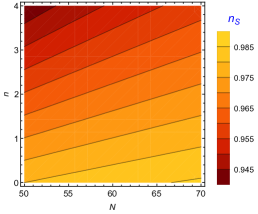
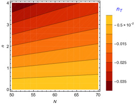
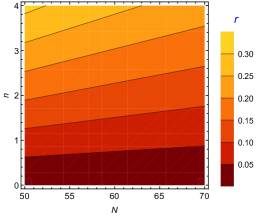
Figure 2: [color online] Inflationary observables for the power-law potential as functions of the power $n$ and the e-folding number, wherein (a) shows the scalar spectral index, $n_{\rm S}$, (b) indicates the tensor spectral index, $n_{\rm T}$, and (c) demonstrates the tensor-to-scalar ratio, $r$.

Table 2: Inflationary observables in the power-law inflation for some values of $n$ and $N$.

$n$	$N$	$n_{\rm S}$	$r$	$n_{\rm T}$
0.5	50	0.97506	0.03990	-0.00498
1.0	50	0.97014	0.07960	-0.00995
1.5	51	0.96593	0.11678	-0.01459
2.0	56	0.96460	0.14159	-0.01769
2.5	62	0.96407	0.15968	-0.01996
3.0	70	0.96466	0.16961	-0.02120
3.5	70	0.96119	0.19753	-0.02469
4.0	70	0.95774	0.22535	-0.02816

V.2 Hyperbolic Potential

In Ref. rubanoandbarrow , an exact hyperbolic form of the scalar field potential has been specified at the spatially flat Friedmann Universe containing a scalar field with equation of state $p^{[\phi]}=\left(\gamma^{[\phi]}-1\right)\rho^{[\phi]}$ and a perfect fluid with equation of state $p^{[\rm m]}=\left(\gamma-1\right)\rho^{[\rm m]}$ (where $\gamma^{[\phi]}=w^{[\phi]}+1$ and $\gamma=w+1$), in terms of $H_{0}$, $\Omega^{[\rm m]}_{0}$, $w$ and $w^{[\phi]}$. Also, dark energy has been discussed with cosmological acceleration from the scalar field with such a potential at the late-time Universe. Moreover, in Ref. hyperbolic , the hyperbolic scalar field potential has been studied in the concept of inflation in GR, which leads to consistent inflationary observables with the Planck $2015$ data for some ranges of $h$ and $b$ parameters, and derives $r\simeq 0.07$ when $26{\rm M_{Pl}}\leq h\leq 39{\rm M_{Pl}}$ and $1.02\leq b\leq 1.1$. In this work, we intend to investigate the hyperbolic potential within the context of $f(Q,T)$ gravity.

The hyperbolic potential can be described as

$$V(\phi)=A\,\sinh^{b}\left(\dfrac{\phi}{h}\right),$$ (94)

where $h$ is scaled as the Planck mass, and the constants $A$ and $b$ have been defined as rubanoandbarrow

$$A\equiv 3H_{0}^{2}\left(1-\Omega^{[m]}_{0}\right)\left(1-\dfrac{\gamma^{[\phi]}}{2}\right)\left(\dfrac{1-\Omega^{[m]}_{0}}{\Omega^{[m]}_{0}}\right)^{-b/2},$$ (95)

$$b\equiv-\dfrac{2\gamma^{[\phi]}}{\gamma-\gamma^{[\phi]}}=\dfrac{2\left(1+w^{[\phi]}\right)}{1+w^{[\phi]}-\gamma}.$$ (96)

In these relations, $H_{0}$ and $\Omega^{[m]}_{0}$ are the value of the present-day Hubble parameter and the present-day matter density parameter, respectively. Obviously, for the radiation-dominated era, the constant $b$ is

$$b=\dfrac{6\left(1+w^{[\phi]}\right)}{3w^{[\phi]}-1}.$$ (97)

Substituting potential (94) into relations (79) and (80) gives the slow-roll parameters for this case to be

$$\epsilon\approx\dfrac{-\alpha\,b^{2}}{2\left(\kappa+\beta\right)h^{2}}\coth^{2}\left(\dfrac{\phi}{h}\right),$$ (98)

$$\eta\approx\dfrac{-\alpha\,b}{\left(\kappa+\beta\right)h^{2}}\dfrac{\left[b\cosh^{2}\left(\dfrac{\phi}{h}\right)-1\right]}{\left[\cosh^{2}\left(\dfrac{\phi}{h}\right)-1\right]}.$$ (99)

Also, by using the end of inflation condition, ${\rm\epsilon}(\phi_{{\rm end}})=1$, we obtain

$$\phi_{{\rm end}}\approx h\times\,{\rm arccoth}\left[\sqrt{\dfrac{-2\left(\kappa+\beta\right)h^{2}}{\alpha\,b^{2}}}\right],$$ (100)

where again $-\alpha/(\kappa+\beta)$ must be positive. Moreover, by inserting potential (94) into relation (81), the e-folding number reads

$$N\approx\dfrac{-h^{2}\left(\kappa+\beta\right)}{\alpha\,b}\ln\left[\dfrac{\cosh\left(\dfrac{\phi}{h}\right)}{\cosh\left(\dfrac{\phi_{\rm end}}{h}\right)}\right].$$ (101)

Consequently, by substituting relation (100) into relation (101), we obtain the scalar field as

$$\phi\approx h\times\,{\rm arccosh}\left[\dfrac{\exp\left(\dfrac{-\alpha\,bN}{\left(\kappa+\beta\right)h^{2}}\right)\sqrt{\dfrac{-2\left(\kappa+\beta\right)h^{2}}{\alpha\,b^{2}}}}{\sqrt{\dfrac{-2\left(\kappa+\beta\right)h^{2}}{\alpha\,b^{2}}-1}}\right],$$ (102)

where $\left[-2\left(\kappa+\beta\right)h^{2}/(\alpha\,b^{2})-1\right]$ must be positive. This condition makes more restriction on $\alpha$ and $\beta$ than the above one (under relation (100)), e.g. it includes [$\alpha>0$ with $\beta<-\kappa-\alpha\,b^{2}/(2h^{2})$] and [$\alpha<0$ with $\beta>-\kappa-\alpha\,b^{2}/(2h^{2})$]. Under these conditions, the slow-roll parameters read

$$\epsilon\approx\dfrac{-\alpha\,b^{2}}{{\rm D}}\exp\left[\dfrac{-2\alpha\,bN}{\left(\kappa+\beta\right)h^{2}}\right],$$ (103)

$$\eta\approx\dfrac{-\alpha b\left\{2h^{2}\left(\kappa+\beta\right)\!\left[b\exp\left(\dfrac{-2\alpha bN}{\left(\kappa+\beta\right)h^{2}}\right)\!-1\right]\!-\alpha b^{2}\right\}}{h^{2}{\rm D}\left(\kappa+\beta\right)},$$ (104)

where

$${\rm D}\equiv 2h^{2}\left(\kappa+\beta\right)\left[\exp\left(\dfrac{-2\alpha bN}{\left(\kappa+\beta\right)h^{2}}\right)-1\right]-\alpha b^{2}.$$ (105)

As a result, the inflationary observables, in this case, obviously are

$$n_{\rm S}\approx 1+\dfrac{6\alpha b^{2}}{{\rm D}}\exp\left(\dfrac{-2\alpha bN}{\left(\kappa+\beta\right)h^{2}}\right)$$

$$-\dfrac{2\alpha b\left\{2h^{2}\left(\kappa+\beta\right)\left[b\exp\left(\dfrac{-2\alpha bN}{\left(\kappa+\beta\right)h^{2}}\right)-1\right]-\alpha b^{2}\right\}}{h^{2}{\rm D}\left(\kappa+\beta\right)},$$ (106)

$$n_{T}\approx\dfrac{2\,\alpha\,b^{2}}{{\rm D}}\exp\left[\dfrac{-2\,\alpha\,b\,N}{\left(\kappa+\beta\right)h^{2}}\right],$$ (107)

$$r\approx\dfrac{-16\,\alpha\,b^{2}}{{\rm D}}\exp\left[\dfrac{-2\,\alpha\,b\,N}{\left(\kappa+\beta\right)h^{2}}\right].$$ (108)

As is clear from these relations, within the framework of the linear functional form of $f(Q,T)$ gravity while considering the hyperbolic scalar field potential, the inflationary observables depend on parameters $b$, $N$ and on a single combination of the other parameters, i.e. $-h^{2}(\kappa+\beta)/\alpha$, with respect to GR. The scaling change

$$h^{2}\kappa\rightarrow\dfrac{h^{2}(\kappa+\beta)}{-\alpha},$$ (109)

stems from relation (82) that leads to the relations resulting from GR with a minimally coupled scalar field (see the Appendix). Such a modification can cause even slight differences compared to the results of the GR case. For instance, to obtain consistent results with the Planck data in GR, the allowed range of $h$ is $h\geq 11.7{\rm M_{Pl}}$ hyperbolic . In this case of linear $f(Q,T)$ gravity, relation(109) can impose different restrictions on the corresponding $h$ value, i.e. $\tilde{h}\geq\sqrt{(\kappa+\beta)/(-\alpha\kappa)}\,11.7{\rm M_{Pl}}$, where we have set $h^{2}\kappa\rightarrow\tilde{h}^{2}\kappa$.

Figs. 3 and 4 show the corresponding inflationary observables of the hyperbolic potential with $N=50$, while considering ($b=1.448$ and $h=18M_{\rm Pl}$) and ($b=1.090$ and $h=25M_{\rm Pl}$) with different values of $\beta$, and negative and positive values of $\alpha$, respectively. Also, some acceptable values of the inflationary observables have been presented in Table 3 for different values of $h$, $b$, $\alpha$, and $\beta$. The results confirm that the inflationary observables in the $f(Q,T)$ gravity while considering the hyperbolic potential are consistent with the latest Planck $2018$ observational data. However, for positive values of $\alpha$, while relaxing the condition $-\alpha/$\kappa+\beta$>0$, we obtain more consistent results with the joint Planck, BK15 and BAO (61). Moreover, it makes $r$ more restrictive than the hyperbolic inflation in GR. Hence, the hyperbolic potential almost leads to a viable $f(Q,T)$ gravity model in the early stage of the Universe.

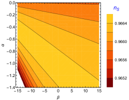
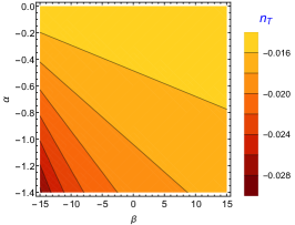
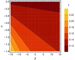
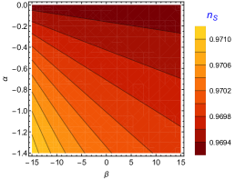
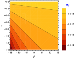
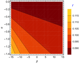
Figure 3: [color online] Inflationary observables for the case of hyperbolic potential as functions of parameters $\alpha<0$ and $\beta$. Top figures have been calibrated with $h=18\,M_{\rm Pl}$, $b=1.448$ and $N=50$, and bottom figures with $h=25\,M_{\rm Pl}$, $b=1.090$ and $N=50$.

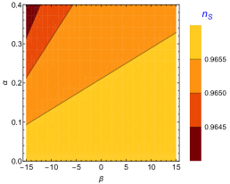
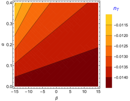
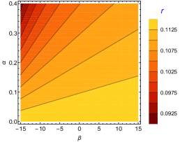
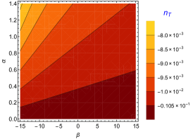
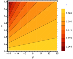
Figure 4: [color online] Inflationary observables for the case of hyperbolic potential as functions of parameters $\alpha>0$ and $\beta$. Top figures have been calibrated with $h=18\,M_{\rm Pl}$, $b=1.448$ and $N=50$, and bottom figures with $h=25\,M_{\rm Pl}$, $b=1.090$ and $N=50$.

Table 3: Inflationary observables in the hyperbolic inflation for some values of $h$, $b$, $\alpha$ and $\beta$. Note that, for some of the given values, the condition $-\alpha/(\kappa+\beta)>0$ is relaxed in order to consider further matter configurations.

$h$ (in $M_{\rm Pl}$)	$b$	$\alpha$	$\beta$	$n_{\rm S}$	$r$	$n_{\rm T}$
14	1.480	0.63	8.74	0.96418	0.09786	-0.01223
14	1.480	-0.97	-7.94	0.96499	0.19206	-0.02400
18	1.448	0.28	-12.81	0.96491	0.10076	-0.01259
18	1.448	-1.31	-13.22	0.96494	0.20090	-0.02511
18	1.448	-1.49	-11.94	0.96479	0.20362	-0.02511
25	1.090	1.21	3.19	0.96832	0.07884	-0.00985
25	1.090	2.51	-10.02	0.96460	0.05879	-0.00734
25	1.090	-0.15	2.51	0.96938	0.08780	-0.01097
25	1.090	-0.53	-7.25	0.96983	0.09253	-0.01156
30	1.009	3.68	-11.35	0.96492	0.05371	-0.00671
30	1.009	4.54	-7.95	0.96498	0.05396	-0.00674
30	1.009	-0.74	3.67	0.97041	0.08090	-0.01041
30	1.009	-0.32	-5.43	0.97029	0.08219	-0.01027
35	1.002	2.21	-19.12	0.96496	0.05313	-0.00664
35	1.002	3.20	-15.74	0.96542	0.05488	-0.00686
35	1.002	4.56	-14.01	0.96416	0.05063	-0.00632
35	1.002	5.83	-8.41	0.96528	0.05442	-0.00680

V.3 Natural Potential

As the last scalar field potential case, we analyze the inflationary observables using the natural potential, which is defined as

$$V(\phi)=\Lambda^{4}\left[1+\cos\left(\dfrac{\phi}{l}\right)\right],$$ (110)

where $\Lambda$ and $l$ are constants with mass dimensions. For successful inflation in such a potential, $l$ is scaled as the Planck mass and $\Lambda$ is scaled as the grand unified mass $M_{\rm GUT}\sim 10^{16}~{}{\rm GeV}$. With the natural potential, inflation naturally takes place and a pseudo-Nambu-Goldstone boson is a responsible field for it natural ; natcob ; partmod . However with this potential, the predictions of GR inflation for the tensor-to-scalar ratio is strongly disfavored by the joint Planck, BK15 and BAO data (61), which motivates to study inflation in the concept of $f(Q,T)$ formalism.

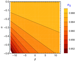
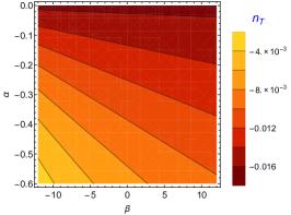
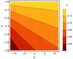
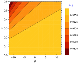
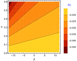
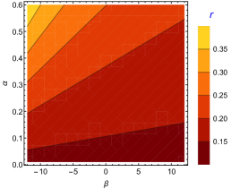
Figure 5: [color online] Inflationary observables for the natural potential as functions of parameters $\alpha$ and $\beta$. Top figures are for $\alpha<0$, and bottom figures for $\alpha>0$. All of these figures have been depicted for $l=5\,M_{\rm Pl}$ and $N=60$.

Table 4: Inflationary observables in the natural inflation for some values of $l$ , $\alpha$ and $\beta$. Note that, for some of the given values, the condition $-\alpha/(\kappa+\beta)>0$ is relaxed in order to consider further matter configurations.

$l$ (in $M_{\rm Pl}$)	$\alpha$	$\beta$	$n_{\rm S}$	$r$	$n_{\rm T}$
3	-0.16	-7.51	0.96069	0.05574	-0.00697
3	-0.20	-2.41	0.96106	0.05743	-0.00717
3	-0.28	4.61	0.96025	0.05388	-0.00673
3	-0.33	10.97	0.96062	0.05543	-0.00692
5	-0.25	-10.05	0.96418	0.07658	-0.00957
5	-0.48	8.42	0.96488	0.08295	-0.01036
5	-0.85	6.76	0.96000	0.05283	-0.03283
5	-1.03	13.61	0.96003	0.05254	-0.00662
5	0.07	-3.56	0.96683	0.14590	-0.01823
8	-0.86	-5.43	0.96402	0.07530	-0.00941
8	-1.12	1.64	0.96426	0.07723	-0.00965
8	-1.32	-5.64	0.96009	0.05322	-0.00942
8	-2.33	10.24	0.96045	0.05472	-0.00684
8	0.87	-1.76	0.96481	0.19920	-0.02490

Similar to the previous cases, the slow-roll parameters for the natural potential are

$${\rm\epsilon}\approx\dfrac{-\alpha}{2\left(\kappa+\beta\right)l^{2}}\dfrac{\sin^{2}\left(\dfrac{\phi}{l}\right)}{\left[1+\cos\left(\dfrac{\phi}{l}\right)\right]^{2}},$$ (111)

$$\eta\approx\dfrac{\alpha}{\left(\kappa+\beta\right)l^{2}}\dfrac{\cos\left(\dfrac{\phi}{l}\right)}{\left[1+\cos\left(\dfrac{\phi}{l}\right)\right]}.$$ (112)

Then, by using condition ${\rm\epsilon(\phi_{\rm end})}=1$, one obtains $\phi_{\rm end}$ as

$$\phi_{\rm end}\approx l\times\,\arccos\left[\dfrac{\alpha+2l^{2}\left(\kappa+\beta\right)}{\alpha-2l^{2}\left(\kappa+\beta\right)}\right],$$ (113)

where the argument of cosine must be $-1<[\alpha+2l^{2}\left(\kappa+\beta\right)]/[\alpha-2l^{2}\left(\kappa+\beta\right)]<1$ that leads once again to condition $-\alpha/(\kappa+\beta)>0$. Moreover, the e-folding number for this potential takes the form

$$N\approx\dfrac{\left(\kappa+\beta\right)l^{2}}{\alpha}\ln\left[\dfrac{1-\cos\left(\dfrac{\phi}{l}\right)}{1-\cos\left(\dfrac{\phi_{\rm end}}{l}\right)}\right].$$ (114)

By substituting relation (113) into relation (114), one can express $\phi$ in terms of the e-folding number as

$$\phi\!\approx\!l\times\arccos\!\left\{\!\dfrac{\alpha\!-2l^{2}\left(\kappa+\beta\right)\!\left[1\!-2\exp\left(\dfrac{\alpha N}{\left(\kappa+\beta\right)l^{2}}\right)\right]}{\alpha-2l^{2}\left(\kappa+\beta\right)}\!\right\}\!,$$ (115)

where $\cos\left(\phi_{\rm end}/l\right)\neq 1$ (that is why we omitted the second equality in the argument of cosine below relation (113)). Under these considerations, the slow-roll parameters are

$${\rm\epsilon}\approx\dfrac{\alpha\exp\left(\dfrac{\alpha N}{\left(\kappa+\beta\right)l^{2}}\right)}{\alpha-2l^{2}\left(\kappa+\beta\right)\left[1-\exp\left(\dfrac{\alpha N}{\left(\kappa+\beta\right)l^{2}}\right)\right]},$$ (116)

$$\eta\approx\dfrac{\alpha\left\{\alpha-2l^{2}\left(\kappa+\beta\right)\left[1-2\exp\left(\dfrac{\alpha N}{\left(\kappa+\beta\right)l^{2}}\right)\right]\right\}}{2l^{2}\left(\kappa+\beta\right)\!\left\{\alpha\!-2l^{2}\left(\kappa+\beta\right)\!\left[1\!-\!\exp\left(\dfrac{\alpha N}{\left(\kappa+\beta\right)l^{2}}\right)\!\right]\right\}}.$$ (117)

Consequently, the inflationary observables obviously read

$$n_{\rm S}\approx 1-\dfrac{6\alpha\exp\left(\dfrac{\alpha N}{\left(\kappa+\beta\right)l^{2}}\right)}{\alpha-2l^{2}\left(\kappa+\beta\right)\left[1-\exp\left(\dfrac{\alpha N}{\left(\kappa+\beta\right)l^{2}}\right)\right]}$$

$$+\dfrac{\alpha\left\{\alpha-2l^{2}\left(\kappa+\beta\right)\left[1-2\exp\left(\dfrac{\alpha N}{\left(\kappa+\beta\right)l^{2}}\right)\right]\right\}}{l^{2}\left(\kappa+\beta\right)\!\left\{\alpha\!-2l^{2}\left(\kappa+\beta\right)\!\left[1\!-\exp\left(\dfrac{\alpha N}{\left(\kappa+\beta\right)l^{2}}\right)\right]\right\}},$$ (118)

$$n_{\rm T}\approx\dfrac{-2\alpha\exp\left(\dfrac{\alpha N}{\left(\kappa+\beta\right)l^{2}}\right)}{\alpha-2l^{2}\left(\kappa+\beta\right)\left[1-\exp\left(\dfrac{\alpha N}{\left(\kappa+\beta\right)l^{2}}\right)\right]},$$ (119)

$$r\approx\dfrac{16\alpha\exp\left(\dfrac{\alpha N}{\left(\kappa+\beta\right)l^{2}}\right)}{\alpha-2l^{2}\left(\kappa+\beta\right)\left[1-\exp\left(\dfrac{\alpha N}{\left(\kappa+\beta\right)l^{2}}\right)\right]}.$$ (120)

As is clear, with the natural potential, these relations depend on the e-folding number and on a single combination of the other parameters, i.e. $-l^{2}$\kappa+\beta$/\alpha$, with respect to GR. The scaling change of the mass scale $l$, i.e.

$$l^{2}\kappa\rightarrow\dfrac{l^{2}(\kappa+\beta)}{-\alpha},$$ (121)

also stems from relation (82) that leads to the relations resulting from GR with a minimally coupled scalar field (see the Appendix). Such a modification can cause some differences compared to the results of the GR case. For instance, the natural inflation can provide Planck:2018jri consistent results with the Planck 2018 data in the case of GR if $0.3<\log_{10}(l/{\rm M_{Pl}})<2.5$ at $95\%\ {\rm CL}$. In this case of linear $f(Q,T)$ gravity, relation (121) can impose different restrictions on the corresponding $l$ value, i.e. $0.3+F<\log_{10}(\tilde{l}/{\rm M_{Pl}})<2.5+F$ where $F\equiv\log_{10}\sqrt{(\kappa+\beta)/(-\alpha\kappa)}$, where we have set $l^{2}\kappa\rightarrow\tilde{l}^{2}\kappa$.

Fig. 5 indicates the scalar spectral index, the tensor spectral index, and the tensor-to-scalar ratio for $N=60$, $l=5\,M_{\rm Pl}$ with different values of $\beta$ and $\alpha$ for the natural potential. Also, Table 4 shows the inflationary observables for different values of $l$, $\alpha$ and $\beta$. The results indicate that, for some ranges of free parameters within the context of the linear functional form of the $f(Q,T)$ gravity with the natural potential, the inflationary observables are in very good agreement with the observational data obtained from the Planck satellite, i.e., data (58). Furthermore, with the natural potential, it is interesting that, for some negative values of $\alpha$ and appropriate $\beta$ (consistent with the related condition), our findings make $r$ even more restrictive and (within the given limits of $n_{S}$) in good agreement with the joint Planck, BK15 and BAO data, i.e. relation (61), in contrast to the results obtained from GR in this case.

VI Conclusions

In recent decades, a wide range of investigations has been performed to describe the dynamics of the Universe. In this regard, the results of studies somehow reflect the fact that the standard model of cosmology derived from GR offers the best description. Nevertheless, the CMB observables contain very important information about the formation and evolution of the Universe, and some fundamental concepts, such as the flatness and horizon problems, still have remained as open issues within the context of the standard model of cosmology. To address these shortcomings, further research on cosmological inflation appears to be needed in the earliest stages of the Universe. However, although GR has made accurate predictions to describe the cosmological phenomena, it is undesirable to justify the effect of dark sectors on the dynamics of the Universe in a way that is well consistent with the observational data. For this purpose, studying alternative models of gravity can be a good motivated.

In this work, we have investigated the cosmological inflation within the context of $f(Q,T)$ gravity. To perform this task, first we have described the simplest theoretical framework for cosmological inflation based on GR with an isotropic and homogeneous scalar field known as inflaton. Then, by assuming the spatially flat FLRW spacetime and a linear barotropic equation of state, we have introduced the slow-roll parameters in terms of the Hubble parameter and its time derivatives. For inflation to occur and have a sufficient time scale as well as timely end of inflation, the conditions $|{\rm\epsilon_{n}}|\ll 1$ and ${\rm\epsilon}=1$ must be satisfied. In addition, to calculate the inflationary parameters in the presence of the scalar field, we have derived the potential representation of slow-roll parameters. We have also applied the slow-roll conditions in the related calculations.

By considering the energy-momentum tensor as a perfect fluid, we have calculated the modified Friedman equations, the effective pressure and energy densities, and the evolution of energy density extracted from $f(Q,T)$ gravity. Furthermore, by choosing a linear combination of $Q$ and $T$, we have shown that the evolution of phantom and quintessence dominated era, that unified two-phase of acceleration of the Universe in the early and late-time, can be achieved in $f(Q,T)$ gravity theory. Also, we have modeled the inflationary scenario for the linear $f(Q,T)$ gravity, and have calculated the slow-roll parameters, the scalar spectral index, the tensor spectral index, and the tensor-to-scalar ratio. The results show that the inflationary quantities within the context of the linear $f(Q,T)$ gravity are independent of the e-folding number and the free parameter $\alpha$. Instead, they depend only on the parameters $\beta$ and $w$. In addition, we have indicated that with the values ($w=-1$ with $\beta\neq-\kappa/2$) and/or ($\beta=-\kappa$ with $w\neq 1$), no inflation could have occurred in the early Universe, and in fact these values represent the expansion phase of de Sitter. Also, for the values ($w=-1$ with $\beta=-\kappa/2$) and/or ($\beta=-\kappa$ with $w=1$), the solution to the field equations is the Minkowski metric with no inflation.

Furthermore, we have investigated the slow-roll inflation in the presence of a scalar field within the context of the linear $f(Q,T)$ gravity, and have calculated the corresponding inflationary observables. We have also computed the inflationary observables for this model with three different cases of inflationary potentials, namely the power-law, the hyperbolic and the natural potentials.

For the power-law potential, the theoretical results indicate that the inflationary observables depend only on the power of the scalar field, $n$, and the e-folding number. We have specified that this potential for the linear $f(Q,T)$ gravity does not lead to further correction to the inflationary observables compared to those ones extracted from GR.

For the case of hyperbolic potential, by fixing the e-folding number and the two parameters of the potential, the related inflationary observables obviously depend only on the free parameters of the linear form, i.e. $\alpha$ and $\beta$. The theoretical results demonstrate that, by considering the hyperbolic potential for the linear $f(Q,T)$ gravity, the appropriate values of inflationary observables can be found to be in good agreement with the observational data obtained from the Planck satellite for some ranges of negative and positive values of $\alpha$. However, while relaxing the condition $-\alpha/$\kappa+\beta$>0$, the positive values of $\alpha$ give even consistent results with the joint Planck, BK15 and BAO data. Furthermore, the contribution of linear $f(Q,T)$ gravity can impose some differences in the restrictions on the parameter of the hyperbolic potential compared to the results obtained for the GR case.

Finally, for the natural potential, again by fixing the e-folding number and the parameter of the potential, the related inflationary observables obviously depend only on the free parameters of the linear form. The theoretical results indicate that, within the context of the linear $f(Q,T)$ gravity with the natural potential, the obtained inflationary parameters are not only in good agreement with the Planck data but (in contrast to the results obtained from GR in this case) also well consistent with the joint Planck, BK15 and BAO observational data, which impose tighter constraint on the value of the tensor-to-scalar ratio. These results justify the use of the $f(Q,T)$ gravity. Furthermore, the contribution of linear model of $f(Q,T)$ gravity can also impose some differences in the restrictions on the parameter of the natural potential compared to the results obtained for the GR case.

Appendix

The symmetric teleparallel gravity has some generalizations, one of which is known as $f(Q,T)$ gravity. In this appendix, we review some prerequisites related to this theory of gravity.

In differential geometry, any general connection (e.g. $\Gamma^{\alpha}{}_{\mu\nu}$) can obviously be decomposed into three independent components as

$$\Gamma^{\alpha}{}_{\mu\nu}=\{^{\alpha}{}_{\mu\nu}\}+K^{\alpha}{}_{\mu\nu}+L^{\alpha}{}_{\mu\nu},$$ (122)

where $\{^{\alpha}{}_{\mu\nu}\}$, $K^{\alpha}{}_{\mu\nu}$ and $L^{\alpha}{}_{\mu\nu}$ respectively are the Christoffel symbol, the contorsion tensor and disformation tensor defined as

$$\{^{\alpha}{}_{\mu\nu}\} = \dfrac{1}{2}g^{\alpha\beta}(\partial_{\mu}g_{\beta\nu}+\partial_{\nu}g_{\beta\mu}-\partial_{\beta}g_{\mu\nu}),$$ (123)

$$K^{\alpha}{}_{\mu\nu} = \dfrac{1}{2}\tau^{\alpha}{}_{\mu\nu}+\tau_{(\mu\nu)}{}^{\alpha},$$ (124)

$$L^{\alpha}{}_{\mu\nu} \equiv -\dfrac{1}{2}g^{\alpha\beta}\left(Q_{\mu\beta\nu}+Q_{\nu\beta\mu}-Q_{\beta\mu\nu}\right),$$ (125)

where $\tau^{\alpha}{}_{\mu\nu}=2\Gamma^{\alpha}{}_{[\mu\nu]}$ is the torsion tensor and $Q_{\alpha\mu\nu}\equiv\nabla_{\alpha}\,g_{\mu\nu}$ is the nonmetricity tensor. In addition, the nonmetricity scalar is defined as

$$Q\equiv-g^{\mu\nu}\left(L^{\alpha}{}_{\beta\mu}L^{\beta}{}_{\nu\alpha}-L^{\alpha}{}_{\beta\alpha}L^{\beta}{}_{\mu\nu}\right).$$ (126)

It is well-known that for a zero Riemann tensor with torsionless case, i.e. a flat manifold, there always exists an adapted coordinate system, in which the connection is zero everywhere. Hence, in such a system, relation (122) leads to

$$L^{\alpha}{}_{\mu\nu}\mathrel{\mathop{=}^{*}}-\{^{\alpha}{}_{\mu\nu}\}.$$ (127)

Subsequently, the nonmetricity scalar (126) in such a system is

$$Q\mathrel{\mathop{=}^{*}}-g^{\mu\nu}\Bigl{(}\{^{\alpha}{}_{\beta\mu}\}\{^{\beta}{}_{\nu\alpha}\}-\{^{\alpha}{}_{\beta\alpha}\}\{^{\beta}{}_{\mu\nu}\}\Bigr{)}$$ (128)

that is exactly equal to minus the effective Einstein-Hilbert Lagrangian (which is not a scalar in this form). Hence, the linear version of $f(Q)$ gravity in the absence of the boundary terms is dynamically equivalent to results of the Einstein-Hilbert action and provides another geometrical formalism for GR. Accordingly, the linear version $f(Q,T)=\alpha\,Q+\beta\,T$ is dynamically equivalent to the linear version $f(R,T)=\alpha\,R+\beta\,T$ theory that is claimed to be the GR case with a slight modification in the matter content Fisher2019 ; HMoraes ; Fisher2020 .

Indeed, the equations of motion of the linear $f(Q,T)=\alpha\,Q+\beta\,T$, wherein $T_{\mu\nu}$ is the usual energy-momentum tensor of a scalar field (e.g. $\phi$), become those of GR with another minimally coupled scalar field (e.g. $\psi$), where

$$\psi=\sqrt{\frac{\kappa+\beta}{-\alpha\kappa}}\,\phi,$$ (129)

with a potential

$$\tilde{V}(\psi)=\frac{\kappa+2\beta}{-\alpha\kappa}V(\phi).$$ (130)

However, this equivalence is a matter of debate, and we intend to justify the use of the linear $f(Q,T)$ gravity by providing a comparison showing possible differences with that obtained from the GR case.

References

- (1) P.G. Ferreira, “Cosmological tests of gravity”, Ann. Rev. Astron. Astrophys. 57, 335 (2019).
- (2) D.N. Spergel et al., “First year Wilkinson Microwave Anisotropy Probe (WMAP) observations: Determination of cosmological parameters”, Astrophys. J. Suppl. 148, 175 (2003).
- (3) D.N. Spergel et al., “Wilkinson Microwave Anisotropy Probe (WMAP) three year results: Implications for cosmology”, Astrophys. J. Suppl. 170, 377 (2007).
- (4) E. Komatsu et al., “Seven-year Wilkinson Microwave Anisotropy Probe (WMAP) observations: Cosmological interpretation”, Astrophys. J. Suppl. 192, 18 (2011).
- (5) G. Hinshaw et al., “Nine-year Wilkinson Microwave Anisotropy Probe (WMAP) observations: Cosmological parameter results”, Astrophys. J. Suppl. 208, 19 (2013).
- (6) Y. Akrami et al., “Planck 2018 results. X. Constraints on inflation”, Astron. Astrophys. 641, A10 (2020).
- (7) N. Aghanim et al., “Planck 2018 results. VI. Cosmological parameters”, Astron. Astrophys. 641, A6 (2020). Erratum: Astron. Astrophys. 652, C4 (2021).
- (8) A.A. Coley and G.F.R. Ellis, “Theoretical cosmology”, Class. Quant. Grav. 37, 013001 (2020).
- (9) A.A. Starobinsky, “A new type of isotropic cosmological models without singularity”, Phys. Lett. B 91, 99 (1980).
- (10) A.H. Guth, “Inflationary universe: A possible solution to the horizon and flatness problems”, Phys. Rev. D 23, 347 (1981).
- (11) A.D. Linde, “A new inflationary universe scenario: A possible solution of the horizon, flatness, homogeneity, isotropy and primordial monopole problems”, Phys. Lett. B 108, 389 (1982).
- (12) A. Albrecht and P.J. Steinhardt, “Cosmology for grand unified theories with radiatively induced symmetry breaking”, Phys. Rev. Lett. 48, 1220 (1982).
- (13) W.J. Percival et al. [2dFGRS], “The 2dF galaxy redshift survey: The power spectrum and the matter content of the universe”, Mon. Not. Roy. Astron. Soc. 327, 1297 (2001).
- (14) H.V. Peiris et al., “First year Wilkinson Microwave Anisotropy Probe (WMAP) observations: Implications for inflation”, Astrophys. J. Suppl. 148, 213 (2003).
- (15) M. Tegmark et al. [SDSS], “The 3-D power spectrum of galaxies from the SDSS”, Astrophys. J. 606, 702 (2004).
- (16) M. Tegmark et al. [SDSS], “Cosmological parameters from SDSS and WMAP”, Phys. Rev. D 69, 103501 (2004).
- (17) M.W. Hossain, R. Myrzakulov, M. Sami and E.N. Saridakis, “Class of quintessential inflation models with parameter space consistent with BICEP2”, Phys. Rev. D 89, 123513 (2014).
- (18) J. Martin, C. Ringeval, R. Trotta and V. Vennin, “The best inflationary models after Planck”, J. Cosmol. Astropart. Phys. 03, 039 (2014).
- (19) C.Q. Geng, M.W. Hossain, R. Myrzakulov, M. Sami and E.N. Saridakis, “Quintessential inflation with canonical and noncanonical scalar fields and Planck 2015 results”, Phys. Rev. D 92, 023522 (2015).
- (20) J. Martin, “The observational status of cosmic inflation after Planck”, Astrophys. Space Sci. Proc. 45, 41 (2016).
- (21) Q.G. Huang, K. Wang and S. Wang, “Inflation model constraints from data released in 2015”, Phys. Rev. D 93, 103516 (2016).
- (22) C.M. Will, “The confrontation between general relativity and experiment”, Living Rev. Rel. 9, 3 (2006).
- (23) M. Ishak, “Testing general relativity in cosmology”, Living Rev. Rel. 22, 1 (2019).
- (24) M. Farhoudi, “On higher order gravities, their analogy to GR, and dimensional dependent version of Duff’s trace anomaly relation”, Gen. Rel. Gravit. 38, 1261 (2006).
- (25) A. De Felice and S. Tsujikawa, “ theories”, Living Rev. Rel. 13, 3 (2010).
- (26) T.P. Sotiriou and V. Faraoni, “ theories of gravity”, Rev. Mod. Phys. 82, 451 (2010).
- (27) S. Nojiri and S.D. Odintsov, “Unified cosmic history in modified gravity: From theory to Lorentz non-invariant models”, Phys. Rep. 505, 59 (2011).
- (28) S. Capozziello and M. De Laurentis, “Extended theories of gravity”, Phys. Rep. 509, 167 (2011).
- (29) T. Clifton, P.G. Ferreira, A. Padilla and C. Skordis, “Modified gravity and cosmology”, Phys. Rep. 513, 1 (2012).
- (30) H. Farajollahi, M. Farhoudi, A. Salehi and H. Shojaie, “Chameleonic generalized Brans-Dicke model and late-time acceleration”, Astrophys. Space Sci. 337, 415 (2012).
- (31) H. Shabani and M. Farhoudi, “Cosmological and solar system consequences of gravity models”, Phys. Rev. D 90, 044031 (2014).
- (32) A. Joyce, B. Jain, J. Khoury and M. Trodden, “Beyond the cosmological standard model”, Phys. Rept. 568, 1 (2015).
- (33) P. Bueno, P.A. Cano, Ó. Lasso A. and P.F. Ramírez, “(Lovelock) theories of gravity”, J. High Energy Phys. 04, 028 (2016).
- (34) R. Zaregonbadi and M. Farhoudi, “Cosmic acceleration from matter-curvature coupling”, Gen. Rel. Gravit. 48, 142 (2016).
- (35) N. Khosravi, “Ensemble average theory of gravity”, Phys. Rev. D 94, 124035 (2016).
- (36) S. Nojiri, S.D. Odintsov and V.K. Oikonomou, “Modified gravity theories on a nutshell: Inflation, bounce and late-time evolution,” Phys. Rept. 692, 1 (2017).
- (37) I. Quiros, “Selected topics in scalar-tensor theories and beyond”, Int. J. Mod. Phys. D 28, 1930012 (2019).
- (38) B. Mishra, S.K. Tripathy and S. Ray, “Cosmological models with squared trace in modified gravity”, Int. J. Mod. Phys. D 29, 2050100 (2020).
- (39) R. Myrzakulov, L. Sebastiani and S. Vagnozzi, “Inflation in -theories and mimetic gravity scenario”, Eur. Phys. J. C 75, 444 (2015).
- (40) M. De Laurentis, M. Paolella and S. Capozziello, “Cosmological inflation in gravity”, Phys. Rev. D 91, 083531 (2015).
- (41) L. Sebastiani, S. Vagnozzi and R. Myrzakulov, “Mimetic gravity: A review of recent developments and applications to cosmology and astrophysics”, Adv. High Energy Phys. 2017, 3156915 (2017).
- (42) M. Tirandari and K. Saaidi, “Anisotropic inflation in Brans-Dicke gravity”, Nucl. Phys. B 925, 403 (2017).
- (43) N. Saba and M. Farhoudi, “Chameleon field dynamics during inflation”, Int. J. Mod. Phys. D 27, 1850041 (2018).
- (44) S.M.M. Rasouli, N. Saba, M. Farhoudi, J. Marto and P.V. Moniz, “Inflationary universe in deformed phase space scenario”, Ann. Phys. 393, 288 (2018).
- (45) S. Chakraborty, T. Paul and S. SenGupta, “Inflation driven by Einstein-Gauss-Bonnet gravity”, Phys. Rev. D 98, 083539 (2018).
- (46) H. Bernardo, R. Costa, H. Nastase and A. Weltman, “Conformal inflation with chameleon coupling”, J. Cosmol. Astropart. Phys. 1904, 027 (2019).
- (47) H.R. Kausar, R. Saleem and A. Ilyas, “Cosmological inflation in f(X) gravity theory”, Phys. Dark Univ. 26, 100401 (2019).
- (48) S. Bhattacharjee, J.R.L. Santos, P.H.R.S. Moraes and P.K. Sahoo, “Inflation in gravity”, Eur. Phys. J. Plus 135, 576 (2020).
- (49) A. Mohammadi, T. Golanbari, J. Enayati, S. Jalalzadeh and K. Saaidi, “Revisiting scalar tensor inflation by swampland criteria and reheating”, arXiv: 2011.13957.
- (50) M. Gamonal, “Slow-roll inflation in gravity and a modified Starobinsky-like inflationary model”, Phys. Dark Univ. 31, 100768 (2021).
- (51) T.Q. Do, “No-go theorem for inflation in Ricci-inverse gravity”, Eur. Phys. J. C 81, 431 (2021).
- (52) E.H. Baffou, M.J.S. Houndjo, I.G. Salako and T. Houngue, “Inflationary cosmology in modified gravity”, Ann. Phys. 434, 168620 (2021).
- (53) M. Faraji, N. Rashidi and K. Nozari, “Inflation in energy-momentum squared gravity in light of Planck 2018”, Eur. Phys. J. Plus 137, 593 (2022).
- (54) S. Bhattacharjee, “Inflation in mimetic gravity”, New Astron. 90, 101657 (2022).
- (55) C.Y. Chen, Y. Reyimuaji and X. Zhang, “Slow-roll inflation in gravity with a mixing term”, arXiv: 2203.15035.
- (56) X. Zhang, C.Y. Chen and Y. Reyimuaji, “Modified gravity models for inflation: In conformity with observations”, Phys. Rev. D 105, 043514 (2022).
- (57) H. Weyl, “Gravitation und elektrizität”, Sitzungsber. Preuss. Akad. Wiss. Berlin, 465 (1918).
- (58) H. Weyl, “Eine neue erweiterung der relativitätstheorie”, Ann. Phys. (Berlin) 59, 101 (1919).
- (59) J.T. Wheeler, “Weyl geometry”, Gen. Rel. Gravit. 50, 80 (2018).
- (60) H. Weyl, “Raum-Zeit-Materie”, (Springer-Verlag, Berlin, 1st ed. 1918, 4th ed. 1921). Its English version (of the 4th ed.) is: “Space-Time-Matter”, translated by: H.L. Brose (Dover Publications, New York, 1st ed. 1922, reprinted 1950).
- (61) P.A.M. Dirac, “Long range forces and broken symmetries”, Proc. R. Soc. London A 333, 403 (1973).
- (62) K. Hayashi, M. Kasuya and T. Shirafuji, “Elementary particles and Weyl’s gauge field”, Prog. Theor. Phys. 57, 431 (1977).
- (63) R. Weitzenböck, “Invariantentheorie”, (Noordhoof, Groningen, 1923).
- (64) J.W. Maluf, “The teleparallel equivalent of general relativity”, Ann. Phys. 525, 339 (2013).
- (65) J.M. Nester and H.J. Yo, “Symmetric teleparallel general relativity”, Chin. J. Phys. 37, 113 (1999).
- (66) J.B. Jiménez, L. Heisenberg and T. Koivisto, “Coincident general relativity”, Phys. Rev. D 98, 044048 (2018).
- (67) J.B. Jiménez, L. Heisenberg and T. Koivisto, “Teleparallel Palatini theories”, JCAP 08, 039 (2018).
- (68) T. Harko, T.S. Koivisto, F.S.N. Lobo, G. J. Olmo and D. Rubiera-Garcia, “Coupling matter in modified gravity” Phys. Rev. D 98, 084043 (2018).
- (69) J. Lu, X. Zhao and G. Chee, “Cosmology in symmetric teleparallel gravity and its dynamical system”, Eur. Phys. J. C 79, 530 (2019).
- (70) J.B. Jiménez, L. Heisenberg, T.S. Koivisto and S. Pekar, “Cosmology in geometry”, Phys. Rev. D 101, 103507 (2020).
- (71) F. D’Ambrosio, L. Heisenberg and S. Kuhn, “Revisiting cosmologies in teleparallelism”, Class. Quant. Grav. 39, 025013 (2022).
- (72) F. D’Ambrosio, S.D.B. Fell, L. Heisenberg and S. Kuhn, “Black holes in gravity”, Phys. Rev. D 105, 024042 (2022).
- (73) S.A. Narawade, L. Pati, B. Mishra and S.K. Tripathy, “Dynamical system analysis for accelerating models in non-metricity gravity”, Phys. Dark Univ. 36, 101020 (2022).
- (74) Y. Xu, G. Li, T. Harko and S.D. Liang, “ gravity”, Eur. Phys. J. C 79, 708 (2019).
- (75) S. Arora, S.K.J. Pacif, S. Bhattacharjee and P.K. Sahoo, “ gravity models with observational constraints”, Phys. Dark Univ. 30, 100664 (2020).
- (76) Y. Xu, T. Harko, S. Shahidi and S.D. Liang, “Weyl type gravity, and its cosmological implications”, Eur. Phys. J. C 80, 449 (2020).
- (77) G. Gadbail, S. Arora and P.K. Sahoo, “Power-law cosmology in Weyl-type gravity”, Eur. Phys. J. Plus 136, 1040 (2021).
- (78) G. Gadbail, S. Arora and P.K. Sahoo, “Viscous cosmology in the Weyl-type gravity”, Eur. Phys. J. C 81, 1088 (2021).
- (79) S. Arora and P.K. Sahoo, “Energy conditions in gravity”, Phys. Scripta 95, 095003 (2020).
- (80) S. Arora, A. Parida and P.K. Sahoo, “Constraining effective equation of state in gravity”, Eur. Phys. J. C 81, 555 (2021).
- (81) S. Arora, J.R.L. Santos and P.K. Sahoo, “Constraining gravity from energy conditions”, Phys. Dark Univ. 31, 100790 (2021).
- (82) N. Godani and G.C. Samanta, “FRW cosmology in f(Q,T) gravity”, Int. J. Geom. Meth. Mod. Phys. 18, 2150134 (2021).
- (83) A. Pradhan and A. Dixit “Transit cosmological models with observational constraints in gravity”, Int. J. Geom. Meth. Mod. Phys. 18, 2150159 (2021).
- (84) L. Pati, B. Mishra and S.K. Tripathy, “Model parameters in the context of late time cosmic acceleration in gravity”, Phys. Scripta 96, 105003 (2021).
- (85) A.S. Agrawal, L. Pati, S.K. Tripathy and B. Mishra, “Matter bounce scenario and the dynamical aspects in gravity”, Phys. Dark Univ. 33, 100863 (2021).
- (86) S. Arora, S.K.J. Pacif, A. Parida and P.K. Sahoo, “Bulk viscous matter and the cosmic acceleration of the universe in gravity”, J. High Energy Astrophys. 33, 1 (2022).
- (87) L. Pati, S.A. Kadam, S.K. Tripathy and B. Mishra, “Rip cosmological models in extended symmetric teleparallel gravity”, Phys. Dark Univ. 35, 100925 (2022).
- (88) P. Rudra, “Energy-momentum squared symmetric teleparallel gravity: gravity”, Phys. Dark Univ. 37, 101071 (2022).
- (89) D.H. Lyth and A. Riotto, “Particle physics models of inflation and the cosmological density perturbation”, Phys. Rept. 314, 1 (1999).
- (90) A.R. Liddle, P. Parsons and J.D. Barrow, “Formalizing the slow roll approximation in inflation”, Phys. Rev. D 50, 7222 (1994).
- (91) V. Mokhanov, “Physicsl Foundations of Cosmology”, (Cambridge University press, Cambridge, 2005).
- (92) J. Martin, C. Ringeval and V. Vennin, “Encyclopædia inflationaris”, Phys. Dark Univ. 5-6, 75 (2014).
- (93) A.R. Liddle, “An introduction to cosmological inflation”, arXiv: astro-ph/9901124.
- (94) D. Baumann, “TASI lectures on inflation”, arXiv: 0907.5424.
- (95) S. Weinberg, “Cosmology”, (Oxford University press, Oxford, 2008).
- (96) R. Myrzakulov, L. Sebastiani and S. Zerbini, “Reconstruction of inflation models”, Eur. Phys. J. C 75, 5 (2015).
- (97) z. Hassan, S. Mandal and P.K. Sahoo, “Traversable wormhole geometries in gravity”, Fortsch. Phys. 69, 6 (2021).
- (98) A.R. Liddle and D.H. Lyth, “Cosmological Inflation and Large-Scale Structure”, (Cambridge University press, Cambridge, 2000).
- (99) D.J. Schwarz, C.A. Terrero-Escalante and A.A. Garcia, “Higher order corrections to primordial spectra from cosmological inflation”, Phys. Lett. B 517, 243 (2001).
- (100) D.H. Lyth and A.R. Liddle, “The Primordial Density Perturbation: Cosmology, Inflation and the Origin of Structure”, (Cambridge University press, Cambridge, 2009).
- (101) A.D. Linde, “Chaotic inflation”, Phys. Lett. B 129, 177 (1983).
- (102) S.A. Pavluchenko, “Some constraints on inflation models with power-law potentials”, Phys. Rev. D 69, 021301(R) (2004).
- (103) C. Rubano and J.D. Barrow, “Scaling solutions and reconstruction of scalar field potentials”, Phys. Rev. D 64, 127301 (2001).
- (104) S. Basilakos and J.D. Barrow, “Hyperbolic inflation in the light of Planck 2015 data”, Phys. Rev. D 91, 103517 (2015).
- (105) K. Freese, J.A. Frieman and A.V. Olinto, “Natural inflation with pseudo Nambu-Goldstone bosons”, Phys. Rev. Lett. 65, 3233 (1990).
- (106) F.C. Adams, J.R. Bond, K. Freese, J.A. Frieman and A.V. Olinto, “Natural inflation: Particle physics models, power law spectra for large scale structure, and constraints from COBE”, Phys. Rev. D 47, 426 (1993).
- (107) D.H. Lyth and A. Riotto, “Particle physics models of inflation and the cosmological density perturbation”, Phys. Rept. 314, 1 (1998).
- (108) C.W. Misner, K.S. Thorne and J.A. Wheeler, “Gravitation”, (Freeman, San Francisco, 1973).
- (109) S.B. Fisher and E.D. Carlson, “Reexamining gravity”, Phys. Rev. D 100, 064059 (2019).
- (110) T. Harko and P.H.R.S. Moraes, “Comment on “Reexamining gravity”, Phys. Rev. D 100, 064059 (2019)”, Phys. Rev. D 101, 108501 (2020).
- (111) S.B. Fisher and E.D. Carlson, “Response to comment on “Reexamining gravity”, Phys. Rev. D 101, 108502 (2020).
- (112) M. Hohmann, “General covariant symmetric teleparallel cosmology”, Phys. Rev. D 104, 124077 (2021).