Electron Temperature Relaxation
in the Clusterized Ultracold Plasmas

Abstract

Ultracold plasmas are a promising candidate for the creation of strongly-coupled Coulomb systems. Unfortunately, the values of the coupling parameter ${\Gamma}_{e}$ actually achieved after photoionization of the neutral atoms remain relatively small because of the considerable intrinsic heating of the electrons. A conceivable way to get around this obstacle might be to utilize a spontaneous ionization of the ultracold Rydberg gas, where the initial kinetic energies could be much less. However, the spontaneous avalanche ionization will result in a very inhomogeneous distribution (clusterization) of the ions, which can change the efficiency of the electron relaxation in the vicinity of such clusters substantially. In the present work, this hypothesis is tested by an extensive set of numerical simulations. As a result, it is found that despite a less initial kinetic energy, the subsequent relaxation of the electron velocities in the clusterized plasmas proceeds much more violently than in the case of the statistically-uniform ionic distribution. The electron temperature, firstly, experiences a sharp initial jump (presumably, caused by the “virialization” of energies of the charged particles) and, secondly, exhibits a gradual subsequent increase (presumably, associated with a multi-particle recombination of the electrons at the ionic clusters). As a possible tool to reduce the anomalous temperature increase, we considered also a two-step plasma formation, involving the blockaded Rydberg states. This leads to a suppression of the clusterization due to a quasi-regular distribution of ions. In such a case, according to the numerical simulations, the subsequent evolution of the electron temperature proceeds more gently, approximately with the same rate as in the statistically-uniform ionic distribution.

I Introduction

Experimental realization of the Coulomb systems with large values of the coupling parameter

$$\Gamma=\frac{q^{2}n^{1/3}}{k_{\rm B}T}$$ (1)

(where $q$, $n$, and $T$ are the electric charge, concentration, and temperature, respectively) is a long-standing problem in plasma physics Ichimaru (1982); Mayorov, Tkachev, and Yakovlenko (1994); Killian (2007). It was usually addressed Fortov and Iakubov (2000) either by shock compression of the substance, resulting in the increased concentration of the charged particles $n$, or by employing the dusty particles with large effective charges $q$.

An absolutely new way for the creation of strongly-coupled plasmas is usage of the very low temperatures $T$, which became possible in the late 1990’s and early 2000’s due to advances in the laser cooling of atoms in the magneto-optical traps Killian et al. (1999); Gould and Eyler (2001); Bergeson and Killian (2003); Killian et al. (2007). These devices were initially constructed for the creation of atomic Bose–Einstein condensates, but later some of them were used for producing the cold ionized gases and studying the respective plasma effects. The main idea Killian et al. (1999) was that, by choosing the energy of a narrow-band ionizing laser slightly above the ionization threshold of cold (almost immobile) atoms, it would be possible to obtain a system of charged particles with very low kinetic energy and, therefore, considerable values of the coupling parameter $\Gamma$.

Besides, the ultracold plasmas could also be formed in the gas-dynamic installations, e.g., the supersonic gaseous jets irradiated by the laser beams Morrison et al. (2008). Such experiments benefit from the much greater gas density achieved, but working with the molecular gases involves a lot of additional complications Aghigh et al. (2020). Yet another (and even earlier) setup for the production of ultracold plasmas were the so-called active space experiments, where the ionized gas clouds were released into the vacuum from spacecraft and after a sharp expansion could also evolve into the ultracold state Dumin (2000, 2001). Unfortunately, the diagnostic facilities in space were very limited as compared to the laboratory installations.

If energy of the absorbed photon is approximately equal to the ionization threshold of the atom, then the released photoelectron will possess zero total energy at infinity (where its velocity tends to zero). Therefore, when the electron is separated from the original atom, e.g., by half the characteristic interionic distance $l/2$ (in other words, it becomes to be governed by the “collective” plasma field), its kinetic and potential energies should be equal to

$$k(l/2)=|u(l/2)|=2\,e^{2}\!/l\,.$$ (2)

In other words,

$${\Gamma}_{e}\approx|u(l/2)|\,/\,k(l/2)=1\,,$$ (3)

i.e., the coupling parameter can be about unity but not substantially larger than this value. (In fact, due to additional heating, e.g., by the three-body recombination, the experimentally-achieved temperature turns out to be a few times greater. So, the coupling parameter ${\Gamma}_{e}$ becomes only a fraction of unity: for example, the recently reported values Chen, Witte, and Roberts (2017) were up to 0.35.)

A natural question arises: Is it possible to overcome the limit (3)? One of the most evident ideas is to irradiate the atoms by photons with energy slightly below the ionization threshold. In such a case, the atoms will not be ionized directly but transferred firstly into the strongly-excited (Rydberg) states. Next, these “inflated” atoms will be ionized spontaneously due to the interparticle interactions. In fact, the effect of spontaneous ionization of the ultracold Rydberg gas and its transformation into the plasma was discovered long time ago Vitrant et al. (1982), and the same phenomenon was observed already in the first experiments with the magneto–optical traps Robinson et al. (2000); Li, Tanner, and Gallagher (2005).

Figure 1: Sketch of the simultaneous scattering of two electrons ($e$) at the ionic cluster, namely, two closely-located ions ($i$), marked by the dotted ring.

At first sight, it can be naturally expected that if the initial energy introduced into the system becomes less, then the resulting electron temperature should be substantially reduced and, therefore, considerable values of the Coulomb coupling parameter, ${\Gamma}_{e}\,{\gg}\,1$, can be achieved. However, a closer analysis reveals the dangerous pitfall: Namely, the ions produced by the spontaneous avalanche ionization will have a strongly nonuniform (clusterized) distribution in space. Then, as illustrated in Fig. 1, such compact ionic clusters (composed, for example, of two particles) will simultaneously attract a few electrons and, thereby, stimulate the inelastic multi-particle scattering, followed by the efficient redistribution of energy between the particles. (As is known, a bi-particle scattering of an electron by the ion cannot result in a noticeable redistribution of energy: it is equivalent to the reflection of a light particle from a “wall”, which can change only direction of the momentum of the scattered particle but not its absolute value and, therefore, the kinetic energy.) So, if multi-particle processes are allowed, the electron temperature can increase substantially.

Yet another factor potentially leading to the increased temperature is that the clusterized ions contribute more to the total value of the potential energy appearing in the virial theorem Landau and Lifshitz (1976) for the system of charged particles. As a result, at the earliest stage of establishment of the quasi-equilibrium energy distribution between the interacting particles (at the time scale about the inverse plasma frequency), the virial value of the kinetic energy should also be larger. We shall discuss the relative contributions of both the above-mentioned effects in more detail in the subsequent sections of the paper.

Therefore, it is unclear in advance if the reduced value of energy introduced initially into the system will lead to the less electron temperature, or it will be quickly compensated by the more violent subsequent relaxation. It is the aim of the present work to answer this question. Let us emphasize that we shall not try to give a self-consistent description of the entire process of the spontaneous ionization. Instead, we shall start from the predefined distributions of ions in space, which are assumed to be formed due to the avalanche ionization, and then study in much detail the subsequent relaxation of the electron velocities in the corresponding ionic configurations.

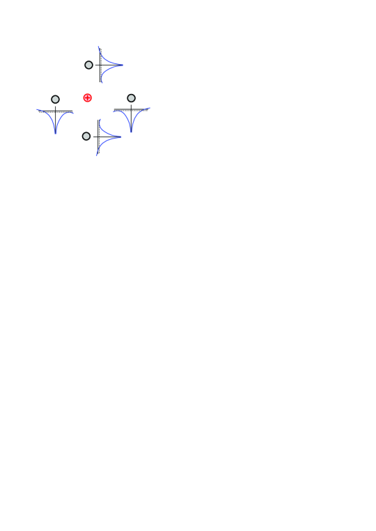
Figure 2: Shift (asymmetry) of the potential curves of atoms in the vicinity of a pre-formed ion, facilitating their subsequent ionization.

Let us briefly mention that, apart from the collisional avalanche ionization, there might be yet another conceivable mechanism of the cluster formation in the case when ions are produced by the near-threshold narrow-band laser irradiation. Namely, the first formed ion shifts the potential curves of nearby atoms, thereby facilitating production of additional ions in the same place; see Fig. 2.

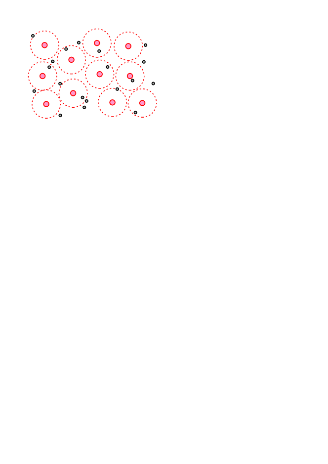
Figure 3: Arrangement of Rydberg atoms (large red circles) in the blockade regime. Dashed rings are the spots of the Rydberg blockade, and small black circles are the unexcited (background) atoms.

One more problem to be addressed in the present paper is treating the case of suppressed clusterization, which can be achieved by the two-step plasma formation with the so-called effect of Rydberg blockade at the first stage, as was suggested in Ref. Robert-de Saint-Vincent et al., 2013. The Rydberg blockade is the phenomenon when one Rydberg atom, excited by a narrow-band laser irradiation, shifts the energy levels of the nearby atoms due to its huge electric dipole moment. As a result, these levels turn out to be beyond the energy band of the irradiation and cannot be excited. So, a subsequent formation of the Rydberg atoms in the neighborhood of the previously excited atom becomes impossible Lukin et al. (2001); Tong et al. (2004); Singer et al. (2004). In principle, if the disturbance is sufficiently strong, the neighboring energy levels can enter the excitation band of irradiation and, thereby, to restore the possibility of excitation to the Rydberg states Keating et al. (2013); Dumin (2014); Derevianko et al. (2015). Moreover, in the case of plasmas, the shift of energy levels can be produced also by the much stronger electric fields of ions. As a result, these levels will either leave or enter the excitation band, thereby leading to the phenomena of Coulomb blockade or anti-blockade, respectively Bounds et al. (2019).

Therefore, as illustrated in Fig. 3, the blockaded Rydberg atoms form a quasi-regular lattice: they are placed approximately at the same distance from each other, so that the possibility of close localization to each other is excluded. If such atoms are subsequently irradiated by an ionizing pulse, then the resulting ions will also possess the quasi-regular arrangement, i.e., their clusterization will be efficiently suppressed. (The atoms that were not initially excited because of the Rydberg blockade remain unionized and do not participate in the plasma processes.)

The experimental attempt to produce plasmas by the two-step process with Rydberg blockade was undertaken, e.g., in Ref. Robert-de Saint-Vincent et al., 2013. Unfortunately, because of the limited diagnostic capabilities, it remained unclear if the electron temperature was really reduced or, in other words, if this is a reasonable approach to the creation of the strongly-coupled ultracold plasmas. So, to answer this question, we shall numerically simulate below both the cases of enhanced and suppressed ionic clusterization.

Besides, the quasi-regular arrangement of ions can be obtained also in the optical lattices, formed by the counter-propagating laser beams. This case was considered in the previous literature mostly in the context of temporal behavior of the ionic coupling parameter ${\Gamma}_{i}$; see, for example, Ref. Murphy and Sparkes, 2016 and references therein. However, it might be interesting to consider also dynamics of electrons in such kind of the ionic background.

At last, a rather sophisticated manipulation with ionic distribution functions can be performed due to specific features of Penning ionization in the molecular Rydberg gases Sadeghi et al. (2014).

II Numerical Simulations

II.1 Formulation of the Model

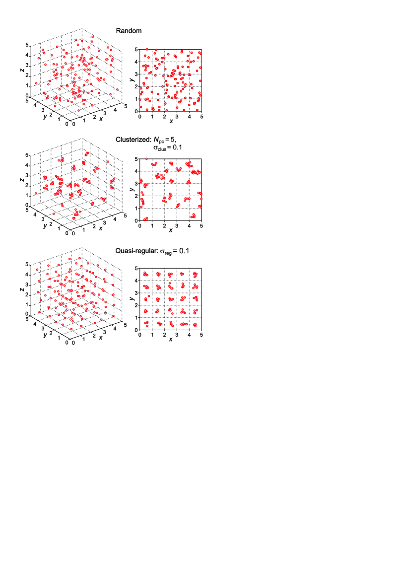
Figure 4: Examples of the ionic arrangement (3D views on the left-hand side, and $xy$-projections on the right-hand side) for the statistically-uniform random distribution (top row), enhanced clusterization with $N_{\rm pc}=5$ and ${\sigma}_{\rm clus}=0.1$ (middle row), and suppressed clusterization with ${\sigma}_{\rm reg}=0.1$ (bottom row). All distances are measured in the units of $l$.

The main idea of subsequent simulations is to consider a relaxation of the electron velocities against the background of immobile ions with various kinds of their arrangement. Namely, the following cases will be tested:

1. Statistically-uniform distribution of ions, where some kind of clusterization is possible only due to occasional coincidence of the ionic coordinates; see Fig. 4 (top row). As an example, we use here a cubic box composed of 5 cells of length $l$ in each direction, where each “unitary” cell (denoted by dotted lines) contains on average exactly one particle.

2. Enhanced clusterization, where each cluster contains $N_{\rm pc}$ ions (the abbreviation “pc” implies “particles per cluster”). To get such an arrangement, we firstly take the centers of the clusters to be distributed statistically uniform in space, and then positions of the individual ions are generated according to the normal (Gaussian) law with the root-mean-square (r.m.s.) deviation ${\sigma}_{\rm clus}$ with respect to the cluster centers; see Fig. 4 (middle row).

3. Suppressed clusterization, where ions were initially located in the nodes of a perfectly regular cubic lattice with the cell size $l$ and then randomly shifted from these positions (randomized) by the normal law with r.m.s. deviation ${\sigma}_{\rm reg}$; see Fig. 4 (bottom row).

The grid of the dotted lines in these figures, denoting the unitary cells, does not have a rigorous physical meaning in the cases of random and clusterized distributions. Nevertheless, this grid is very convenient for the visualization of the average density: each cell corresponds on the average just to one particle.

In the numerical simulations, we used various values of the parameters $N_{\rm pc}$, ${\sigma}_{\rm clus}$, and ${\sigma}_{\rm reg}$, which will be specified below. Besides, for each particular set of these parameters, the simulations were performed for the sufficiently large number of initial conditions (usually, 15) to make the results statistically significant.

Let us mention that the pictures of ionic arrangement are clearly distinct from each other only at the relatively small values of r.m.s. deviations ${\sigma}_{\rm clus}$ and ${\sigma}_{\rm reg}$, e.g., 0.1 (in the units of the interparticle distance $l$), as in Fig. 4. On the other hand, when the r.m.s. deviations are on the order of unity, both the clusterized and quasi-regular distributions become quite similar to the random one. Moreover, as will be seen from the results of subsequent numerical simulations, the electron dynamics in such cases will also be almost the same.

Figure 5: Histograms of the interparticle separation for various kinds of ionic arrangement.

At last, it is interesting to look at the histograms of interparticle separation (i.e., up to normalization, the pair correlation functions), which are presented in Fig. 5. As should be expected, these histograms are strikingly different from each other at small values of the r.m.s. deviation (especially, at $\sigma\,{=}\,0.01)$. On the other hand, the histograms become very similar at the large value of $\sigma$ (namely, $\sigma\,{=}\,1.0$): in this case, all particles are randomly shifted from their original positions by the distances comparable to the average interparticle separation. As a result, all distributions are quasi-random, and their histograms take the Gaussian-like shape.

In the case of quasi-regular distributions with small ${\sigma}_{\rm reg}$, the histograms are very spiky, since the quasi-regular arrangement of particles assumes a large set of the preferable distances between them, exactly as in a crystalline structure. Of course, when ${\sigma}_{\rm reg}$ increases (i.e., the distribution is randomized), these spikes gradually disappear. The most surprising fact is that, even when the entire distribution is very spiky, this actually does not affect the relaxation of electron velocities, as will be seen from the results of numerical simulations below.

On the other hand, a specific feature of the clusterized distributions is a narrow bump (local maximum) at very small distances, on the order of the typical scatter of particles inside the cluster ${\sigma}_{\rm clus}$. While such a bump often looks like a minor disturbance of the histogram, as will be seen from the subsequent simulations, it changes dramatically the efficiency of relaxation of the electron velocities due to the effect of multi-particle scattering, illustrated in Fig. 1.

So, to simulate dynamics of the electrons against the above-mentioned ionic backgrounds, we performed a straightforward numerical integration of their equations of motion:

$$\frac{d^{2}}{dt^{2}}\,{\bf r}_{i}=-\sum_{j}e^{2}\frac{{\bf r}_{i}-{\bf R}_{j}}{|{\bf r}_{i}-{\bf R}_{j}|^{3}}+\sum_{k\neq i}e^{2}\frac{{\bf r}_{i}-{\bf r}_{k}}{|{\bf r}_{i}-{\bf r}_{k}|^{3}}\,,$$ (4)

where ${\bf r}_{i}$ and ${\bf R}_{i}$ are the coordinates of electrons and ions respectively, and $e$ is the elementary electric charge. Since we are interested only in the sufficiently short time scales, the ionic motion was ignored (i.e., the ions were assumed to be at rest at the time interval of the simulation).

While the initial arrangement of ions was outlined above, the initial coordinates of electrons were always specified by a uniform statistical distribution; and their velocities, by the normal (Gaussian) distribution with r.m.s. deviation ${\sigma}_{\!v}$. In the particular simulations presented below, we used ${\sigma}_{\!v}=0.3$, which means that the initial kinetic energy of electrons was an order of magnitude less than their potential (Coulomb) energy. So, the plasma at $t\,{=}\,0$ was assumed to be “overcooled”.

Strictly speaking, the random initial positions for the electrons are somewhat artificial. In the case of instantaneous photoionization, the electron positions should be initially strongly correlated with the positions of ions; and just this case was simulated in detail in the work Niffenegger, Gilmore, and Robicheaux (2011). On the other hand, if the ionization process takes some time, the released electrons will be mixed in space between the ions. So, one can expect that their positions might be reasonably described by the uniform random distribution. As follows from the comparison of our subsequent results with the above-cited paper, a temporal dependence of the kinetic energy turns out to be qualitatively the same, apart from the very early time interval (about the inverse plasma frequency).

For simplicity, the perfectly reflective conditions were imposed at the boundaries of the simulation box. As an alternative, we tried to use also the periodic boundary conditions. Unfortunately, they required a much more computational time to get the convergent results, which was unacceptable in the present study; for more details, see Appendix A.

Of course, for the simulation with a relatively small number of particles within a box with reflective boundaries to correspond to the physical reality, it is necessary that the Debye screening length $r_{\rm D}$ be much smaller than the box size $L$. Since $r_{\rm D}/l=\sqrt{K/6\pi U}$ (where $K=(3/2)\,k_{\rm B}T_{e}$ is electron kinetic energy and $U\approx e^{2}/l$  is the potential one) and $L=5\,l$, one can easily find that at the initial instant of time, when we specified $K\approx 0.1\,U$, the above-mentioned ratio was $r_{\rm D}/L\approx 0.015$. Next, when the electrons are heated in the course of their subsequent dynamics, the temperature can increase by 300 times, up to $K\approx 30\,U$ (see Table 1 and Fig. 8 below). Then, $r_{\rm D}/L\approx 0.26\ll 1$, i.e., the required inequality is still satisfied.

The set of equations (4) was integrated by the numerical algorithm with the adaptive stepsize control, based on the combination of Runge–Kutta methods of the 4th and 5th order (subroutines odeint, rkck, and rkqs from the book Press et al. (1992)). This enabled us to deal with the “original” (singular) Coulomb potentials, without any artificial cut-off or “softening” at the very small distances, e.g. Refs. Niffenegger, Gilmore, and Robicheaux, 2011; Tiwari, Shaffer, and Baalrud, 2017. Thereby, all artifacts caused by the distorted potentials were completely excluded. In this sense, our simulation follows the recent works Venkatesh and Robicheaux (2020); Bobrov et al. (2020); Bronin et al. (2021) as well as our earlier study Dumin (2011). However, despite dealing with the singular functions, the adaptive stepsize control provided us the accuracy of integration (e.g., estimated by the conservation of energy) at the same level as in the majority of other simulations of ultracold plasmas with softened or truncated potentials. Namely, the error was usually about 0.1% and very rarely increased up to 5%.

To check the accuracy of simulations, we tried to perform calculations with various number of particles in the simulation cell. The major part of our results for the variety of initial parameters presented below were obtained for the case of only $N_{\rm tot}=125$ electrons and 125 ions, i.e., exactly for the situation illustrated in Fig. 4. Increasing the number of particles, e.g., up to $N_{\rm tot}=1000$ requires much more computational time (which scales approximately as $N_{\rm tot}^{2}$), but the resulting average curves remain almost the same; for more details, see Appendix B. This is in accordance with the earlier study Niffenegger, Gilmore, and Robicheaux (2011), where a hundred of particles of each kind were found to be sufficient to simulate the electron temperature with a reasonable accuracy.

For the sake of brevity, we shall use below the dimensionless quantities, normalized to the following basic units: the unit of length is the size of the “unitary” cell (or mean distance between the ions) $l$; the unit of time is inversely proportional to the square root of the plasma frequency, $\tau=\sqrt{ml^{3}/e^{2}}=\sqrt{4\pi}/{\omega}_{\rm pl}$; and the unit of energy is the characteristic Coulomb energy, $U=e^{2}/l$. The corresponding normalized quantities will be denoted by hats.

We shall assume below that the electron kinetic energy per particle $K$ (with coefficient 2/3) is a direct measure of the electron temperature $T_{e}$. It was found in Ref. Niffenegger, Gilmore, and Robicheaux, 2011 that such definition of $T_{e}$ reasonably coincides with a more sophisticated derivation of $T_{e}$ by fitting the simulated velocity distributions to the Maxwellian ones, provided that the electrons located sufficiently close to ions (within the “exclusion sphere”) are not taken into account in calculation of the kinetic energy. In fact, as was discussed in our earlier work Dumin (2001), the straightforward definition $T_{e}=(2/3)\,K/k_{\rm B}$ should work rather well even for the electrons strongly interacting with ions. Besides, the introduction of the exclusion spheres is not a self-consistent procedure: a small distance of an electron from the nearby ion at some instant of time cannot be a criterion of its capture by this ion. This is the reason why we take into account all electrons in calculation of the kinetic energy.

II.2 Results of the Numerical Calculations

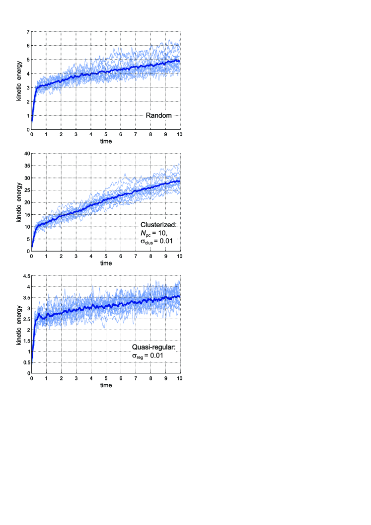
Figure 6: Examples of the temporal behavior of the electron kinetic energy in the case of the purely random ionic distribution (top panel), enhanced clusterization of ions (middle panel), and the suppressed clusterization (bottom panel). Thin blue curves show the individual simulations with different initial conditions for $N_{\rm tot}=125$ particles of each kind, and the thick curve is their average over 15 realizations.

Examples of the computed temporal behavior of the electron kinetic energy for various kinds of ionic arrangement are shown in Fig. 6. To avoid cluttering the figure with a lot of sharp peaks, caused by the close passages of electrons near the ions, the data were smoothed out over the running window of width ${\Delta}\hat{t}=0.1$.

In the case of purely random ionic distribution (top panel), this energy quickly jumps approximately up to the virial value at the time scale $\hat{t}\sim 0.5$, which is in agreement with the pioneering work Kuzmin and O’Neil (2002), as well as with our earlier simulations Dumin (2011). At longer times, the energy continues to increase but much more slowly, due to the heat release by the three- (or multiple-)body recombination, when some electrons become permanently captured by ions.

Next, in the case of considerable clusterization (e.g., $N_{\rm pc}=10,{\sigma}_{\rm clus}=0.01$, middle panel), both the initial jump of energy is a few times greater, and its subsequent increase is much more pronounced. Both these features are not surprising: Really, since the potential energy of compact clusters is larger than in the random distribution, the kinetic energy established after the “virialization” (i.e., after the first stage of relaxation) should be also larger. Besides, since the above-mentioned ionic clusters act as the multiply-charged centers of attraction for a few electrons (see Fig. 1), the efficiency of the three- and multiple-body recombination should also increase, leading to more pronounced heating at the second stage. Naturally, the total increase of the electron temperature becomes larger for the clusters with larger number of ions $N_{\rm pc}$ and the smaller size ${\sigma}_{\rm clus}$, as will be seen below in Fig. 7.

At last, behavior of the electron kinetic energy for the suppressed clusterization of ions (bottom panel) looks quite similar to the case of the purely random distribution. In fact, the resulting values of the electron temperature are a bit smaller than for the random distribution; but this difference is not so significant. A very nontrivial finding of our simulations is that the above-mentioned similarity with random distribution persists even at the very small values of ${\sigma}_{\rm reg}$, corresponding to the almost regular (weakly distorted) ionic lattices.

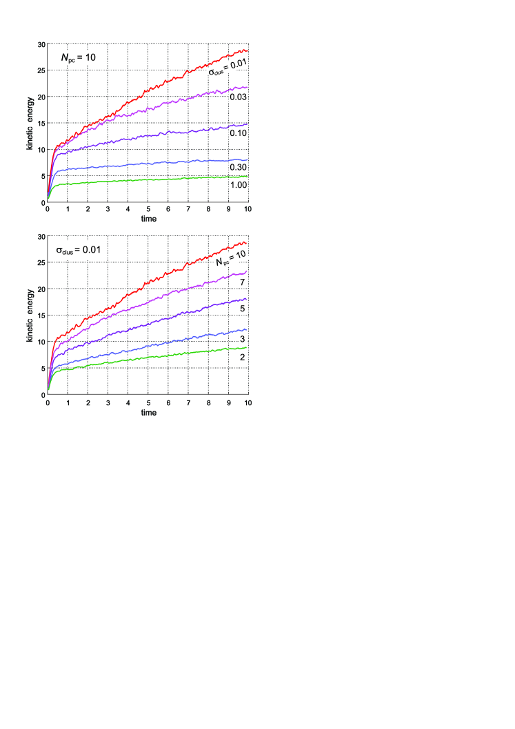
Figure 7: The average (over 15 realizations) temporal behavior of the electron kinetic energy at the fixed $N_{\rm pc}{=}10$ and various ${\sigma}_{\rm clus}$ (top panel) and, vice versa, the fixed ${\sigma}_{\rm clus}{=}0.01$ and various $N_{\rm pc}$ (bottom panel).

To study the case of enhanced clusterization in more detail, it is insightful to plot simultaneously the curves of kinetic energy at the fixed number of particles per cluster $N_{\rm pc}$ (e.g., 10) and various ${\sigma}_{\rm clus}$ (namely, 1, 0.3, 0.1, 0.03, and 0.01), on the one hand, and the same curves at the fixed r.m.s. deviation of particles from the cluster center ${\sigma}_{\rm clus}$ (e.g., 0.01) and various $N_{\rm pc}$ (namely, 2, 3, 5, 7, and 10), on the other hand. As is seen in the top panel of Fig. 7, when $N_{\rm pc}$ is constant and ${\sigma}_{\rm clus}$ decreases from 1 to 0.03 (i.e., the clusters become more compact), the initial jump of temperature (at the time interval from 0 to approximately 0.3) considerably increases, but the subsequent heating (at $\hat{t}\gtrsim 0.3$) changes not so appreciably. However, when ${\sigma}_{\rm clus}$ decreases further to 0.01, the initial jump is “saturated”, but the subsequent heating begins to operate more efficiently.

On the other hand, as is seen in the bottom panel of Fig. 7, when ${\sigma}_{\rm clus}$ is constant while the number of particles per cluster $N_{\rm pc}$ increases from 2 to 10, then both the initial jump of the temperature and the subsequent slope of the curves increase simultaneously.

Finally, the most interesting item for the possibility of creation of the strongly-coupled plasmas are the resulting values of the electron kinetic energy $\langle\hat{K}\rangle$ after a sufficiently long period of evolution. So, it is insightful to plot these values as function of $N_{\rm pc}$ and ${\sigma}_{\rm clus}$. Figure 8 represents the corresponding quantities averaged over the time interval $\hat{t}\in[9,10]$ (which was taken somewhat arbitrary) and 15 different versions of initial conditions. The same data are listed in more detail in Table 1. Strictly speaking, parameter $\sigma$ is irrelevant to the purely random distribution. Nevertheless, the corresponding data are formally placed in the column with ${\sigma}_{\rm reg/clus}=1$, because in this case both the clusterized and quasi-regular distributions become very similar to the random one. To characterize “stability” of the average values, both the r.m.s. deviations with respect to time (over the above-specified interval) $\hat{\sigma}_{t}$ and with respect to different versions of the initial conditions $\hat{\sigma}_{\rm ver}$ are presented there. As is seen, the values of $\hat{\sigma}_{t}$ are usually (but not always) somewhat larger than $\hat{\sigma}_{\rm ver}$. To avoid cluttering Fig. 8, only $\hat{\sigma}_{\rm ver}$ are plotted by the vertical bars.

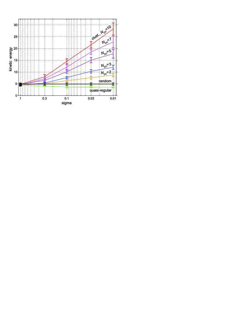
Figure 8: Resulting values of the electron kinetic energy (in dimensionless units), formed at the interval $\hat{t}\in[9,10]$, for various types of the background ionic distribution. Here, $\sigma$ implies either ${\sigma}_{\rm clus}$ or ${\sigma}_{\rm reg}$, depending on the particular context; and their values are plotted in the decreasing order. Vertical bars denote the r.m.s. deviations over the various versions of initial conditions $\hat{\sigma}_{\rm ver}$.

Table 1: Values of the electron kinetic energy $\langle\hat{K}\rangle\pm\hat{\sigma}_{t}\pm\hat{\sigma}_{\rm ver}$ achieved in the interval $\hat{t}\in[9,10]$, where $\hat{\sigma}_{t}$ is the r.m.s. deviation with respect to time, and $\hat{\sigma}_{\rm ver}$ with respect to various versions of initial conditions

	${\sigma}_{\rm reg/clus}$		0.01	0.03	0.10	0.30	1.00
	Random		———————	———————	———————	———————	$4.87{\pm}0.72{\pm}0.57$
	Quasi-regular		$3.50{\pm}0.61{\pm}0.29$	$3.60{\pm}0.66{\pm}0.35$	$3.66{\pm}0.63{\pm}0.46$	$3.99{\pm}0.64{\pm}0.24$	$4.35{\pm}0.60{\pm}0.43$
	Clusterized:	$N_{\rm pc}\!=2$	$8.70{\pm}1.15{\pm}0.75$	$7.57{\pm}1.03{\pm}0.69$	$6.31{\pm}0.83{\pm}0.57$	$5.07{\pm}0.68{\pm}0.44$	$4.42{\pm}0.72{\pm}0.28$
		$N_{\rm pc}\!=3$	$12.03{\pm}1.83{\pm}0.94$	$10.30{\pm}1.23{\pm}0.80$	$7.66{\pm}0.80{\pm}0.53$	$5.31{\pm}0.63{\pm}0.40$	$4.43{\pm}0.64{\pm}0.30$
		$N_{\rm pc}\!=5$	$17.75{\pm}2.46{\pm}1.97$	$15.03{\pm}1.72{\pm}1.17$	$10.12{\pm}1.04{\pm}0.77$	$6.43{\pm}0.83{\pm}0.65$	$4.85{\pm}0.71{\pm}0.44$
		$N_{\rm pc}\!=7$	$22.79{\pm}2.89{\pm}2.54$	$18.51{\pm}1.86{\pm}1.10$	$12.10{\pm}1.29{\pm}1.01$	$7.16{\pm}0.74{\pm}0.78$	$4.56{\pm}0.70{\pm}0.46$
		$N_{\rm pc}\!=10$	$28.29{\pm}3.52{\pm}2.64$	$21.56{\pm}2.02{\pm}1.44$	$14.54{\pm}1.35{\pm}1.18$	$7.99{\pm}0.69{\pm}0.98$	$4.80{\pm}0.63{\pm}0.46$

The quite large values of $\hat{\sigma}_{t}$ and $\hat{\sigma}_{\rm ver}$ were actually caused by the relatively small number of the simulated particles. If this number is increased (e.g., from $N_{\rm tot}=125$ to 1000 particles of each kind), the r.m.s. deviations become much smaller, but the average values almost do not change; for more details, see Appendix B.

III Discussion and Conclusions

As distinct from a number of previous theoretical studies of the avalanche ionization, which were based on the kinetic rate equations (e.g., review Aghigh et al. (2020)), we performed a self-consistent ab initio modeling of the many-body effects in the plasmas with a nontrivial ion arrangement. (It is interesting to mention that already the pioneering work on the avalanche ionization of Rydberg gas Vitrant et al. (1982) emphasized that “it is thus possible that the two-body analysis is too naive”.) Thereby, we arrived at the following conclusions:

1. Studying both the cases of enhanced and suppressed clusterization, in general, reveals the same features as in the previous works: if system of the charged particles is taken initially in the state with very small kinetic energy (e.g., by an order of magnitude less than the potential one), then the kinetic energy begins to increase quickly. This process proceeds in two stages: Firstly, the electrons are sharply accelerated in the local electric fields of the nearby ions and, thereby, increase their kinetic energy approximately up to the virial value (i.e., about a half of the potential one). This takes place on the time scale about the inverse plasma frequency ${\omega}_{\rm pl}$ or, up to the numerical factor, the Keplerian period (more exactly, $\hat{t}\approx$ 0.3). Next, the process of three- or multi-body recombination comes into play, resulting in the subsequent gradual increase of the electron kinetic energy.

2. As follows from Fig. 7, both stages of heating proceed more intensively with increasing the number of particles (ions) per cluster $N_{\rm pc}$ and decreasing the characteristic cluster size ${\sigma}_{\rm clus}$. Besides, according to the top panel of this figure, when $N_{\rm pc}$ is fixed, the increasing compactness of the clusters results initially in more intense virialization (i.e., a sharper jump of the kinetic energy at small $\hat{t}$) and then to the more efficient heating due to the multi-particle recombination, i.e., a steeper increase of the kinetic energy at the second stage. (To avoid misunderstanding, let us emphasize that—although we do not take into account motion of the ions during the simulations—the virial relations should be applied to the total Coulomb energy of all charged particles, i.e. the increased compactness of ionic clusters should be of primary importance.) Of course, the total increase of the kinetic energy at the sufficiently large times (e.g., $\hat{t}\in[9,10]$) will depend on $N_{\rm pc}$ and ${\sigma}_{\rm clus}$ in the same way; see Fig. 8.

3. A very nontrivial finding of our simulations is that a suppressed clusterization (modeled by the quasi-regular ionic distributions) hardly affects the relaxation of the electron velocities. As demonstrated by the lowest curve in Fig. 8, the electron kinetic energy in the interval $\hat{t}\in[9,10]$ remains almost the same when the r.m.s. shift of the ions from the regular lattice positions ${\sigma}_{\rm reg}$ decreases by two orders of magnitude, from 1 to 0.01; and it equals approximately the value for a purely random distribution of ions. Let us emphasize that this conclusion refers only to the electron temperature, while ionic temperature at the longer time scale can exhibit a much more nontrivial behavior, depending on the degree of disorder Pohl, Pattard, and Rost (2004, 2005); Donkó (2009); Murphy, Scholten, and Sparkes (2015); Murphy and Sparkes (2016). Particularly, suppression of the disorder-induced heating of ions, e.g., by the Rydberg blockade of the original gas can be really efficient.

4. Referring to the histograms of interparticle separation (or, which is the same, the pair correlation functions) in Fig. 5, we see that at ${\sigma}_{\rm clus}={\sigma}_{\rm reg}=1$ the plots are approximately Gaussian. This is not surprising because at ${\sigma}_{\rm clus}=1$ the clusters become very diffuse, and at ${\sigma}_{\rm reg}=1$ the original regular lattice becomes completely destroyed. Therefore, these random distributions become statistically uniform in space, and the resulting values of the electron kinetic energy, presented in Fig. 8 and Table 1, are almost the same. Next, when for the clusterized distribution ${\sigma}_{\rm clus}$ decreases, the Gaussian shape of the plots is slightly distorted, and a very narrow peak is formed near zero (i.e., at the very small interparticle separation). In fact, just this peak is of crucial importance for the electron heating, because it strongly enhances both the efficiency of initial virialization and the subsequent multi-body recombination. On the other hand, when for the quasi-regular distribution ${\sigma}_{\rm reg}$ decreases from 1 to 0.01, the Gaussian shape of the plots becomes completely distorted, and a lot of the narrow peaks are formed at various interparticle separations. However, none of these peaks is localized near zero and, as a result, they are insignificant for relaxation of the electron velocities.

5. The main conclusion following from our simulations is that the clusterization of ions (e.g., in the course of avalanche ionization) is a very serious obstacle to getting large values of the Coulomb coupling parameter ${\Gamma}_{e}$. Really, since all energies were normalized to the characteristic Coulomb energy of interparticle interaction (i.e., $\langle\hat{U}\rangle\sim 1$), large values of the dimensionless kinetic energy $\langle\hat{K}\rangle$ obtained in the simulations imply that the coupling parameter ${\Gamma}_{e}\approx U/K=\hat{U}/\hat{K}$ will be rather small as compared to unity. Therefore, the smaller energy input into the Rydberg gas (as compared to the direct photoionization) will lose any advantage after formation of clusters in the spontaneously-ionized plasma. (Yet another conceivable method to reduce the electron temperature in ultracold plasmas is to add there the Rydberg atoms with binding energies $|E_{\rm b}|\lesssim(2-3)\,k_{\rm B}T_{e}$. Then, their inelastic collisions with electrons will lead to a further excitation of the atoms and cooling of the electrons. Unfortunately, as follows both from the experiments and numerical simulations Vanhaecke et al. (2005); Crockett et al. (2018), the overall efficiency of such process is quite low—the electron temperature can be reduced by no more than 20–30 %.)

6. At last, if the two-step formation of ultracold plasma involves the Rydberg blockade at the first stage, resulting in the quasi-regular arrangement of ions Robert-de Saint-Vincent et al. (2013), the electron temperature and the corresponding Coulomb coupling parameter ${\Gamma}_{e}$ should be stabilized approximately at the same level as for the purely random ionic distribution. Therefore, one should not expect that this method can appreciably increase the attainable values of the coupling parameter.

Author Declarations

Conflict of Interest

The authors have no conflicts to disclose.

Author Contributions

YVD suggested the theoretical concept and developed the corresponding software; both authors performed the simulations, analyzed the results, and prepared the manuscript.

Data Availability

The data that support the findings of this study are available from the corresponding author upon reasonable request.

Appendix A Effect of the Boundary Conditions on the Results of Simulations

Since we performed all simulations with a relatively small number of charged particles, it is of crucial importance to specify the adequate boundary conditions. At the first sight, the most reasonable choice would be the periodic conditions, when a particle leaving the simulation box through some boundary simultaneously enters this box from the same point at the opposite boundary. Unfortunately, our computations with periodic boundary conditions led to the quite unsatisfactory results, whose example is presented in Fig. 9. Namely, there was a huge scatter between the individual curves, so that it was meaningless to draw the average curve as in Fig. 6.

Figure 9: Examples of the temporal behavior of the electron kinetic energy in the case of periodic boundary conditions.

A more careful analysis shows that the accumulation of errors (estimated by conservation of the total energy) comes mostly from the transposition of particles between the opposite boundaries, while accuracy of the integration algorithm itself remains very good; see Fig. 10. In fact, the spread of curves in Fig. 9 is caused by a population of the “transient” particles. They are strongly accelerated at the very early stage of plasma relaxation, when almost immobile electrons begin to fall onto the nearest ions. Subsequently, these “transient” electrons cross the boundaries of the simulated volume many times, thereby accumulating the computational errors due to the jumps of the Coulomb forces and energies during the transpositions.

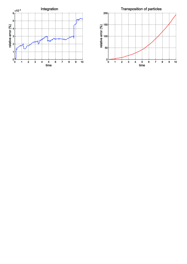
Figure 10: Example of accumulation of the errors due to the integration itself (left panel) and due to the transposition of particles (right panel) in one of the worst cases of initial conditions.

One possible remedy to exclude such errors is to increase the number of “mirror” boxes $N_{\rm m}$ in each direction from the “basic” box, until the required accuracy of convergence of the Coulomb force and energy is achieved. This seems to be the most self-consistent method to take into account the long-range character of the Coulomb interactions. Particularly, just this approach was implemented in one of our earlier works Dumin (2011). Unfortunately, it is extremely time-consuming: the total number of the mirror boxes to be included into the calculations scales with $N_{\rm m}$ as $(2N_{\rm m}+1)^{3}$. As follows from our previous experience Dumin (2011), the required value of $N_{\rm m}$ at a particular step of integration changed from 9 to 27, leading to the total number of mirror boxes to be processed about ${10^{4}}-{10^{5}}$. As a result, the entire simulation for a single set of initial conditions took up to a few months of computational time. Such computing requirements were evidently unacceptable in the present work, because we aimed to perform simulations for a very large set of initial conditions. Therefore, we chose the reflective boundary conditions, where all calculations (both integration of the equations of motion and the summation of the Coulomb interactions) are performed within a single simulation box.

An alternative option might be to employ the “wrap” boundary conditions Niffenegger, Gilmore, and Robicheaux (2011), where any particle interacts with other particles within the cube of size $\pm L/2$ centered at that particle. It can be easily shown that such prescription ensures a smooth variation of the Coulomb energy when the above-mentioned cube is redefined in the course of interparticle displacements. However, the corresponding Coulomb force experiences an abrupt unphysical change (namely, its component perpendicular to the cube boundary suddenly changes its sign for the particular pair of particles). Moreover, the effect of such jumps cannot be represented by the error estimated from the conservation of energy.

In summary, none of the boundary conditions for simulation of the infinite system is perfect: each of them has its own advantages and disadvantages. Anyway, we preferred to use here the reflective boundary conditions because the abrupt changes in velocity, caused by the reflection, have a much more physical meaning than the abrupt changes in the Coulomb forces.

Appendix B Effect of the Number of Particles on the Results of Simulations

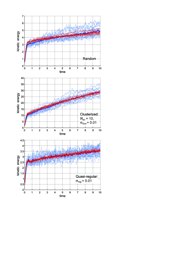
Figure 11: The same as in Fig. 6, but with the results of 5 simulations for $N_{\rm tot}=1000$ particles (red curves) superimposed onto the results of 15 simulations for $N_{\rm tot}=125$ particles (blue curves). The thin and thick curves show the individual simulations and the average results, respectively.

Yet another important issue for the validity of simulations is to check that the results depend only weakly on the total number of particles. With this aim in view, we increased the size of the simulated box from $L=5\,l$ to $L=10\,l$ and, respectively, the number of particles from $N_{\rm tot}=125$ to 1000, i.e., almost by an order of magnitude. The computations were repeated for 5 versions of initial conditions in each of the three extreme cases: a completely random distribution of ions, the most clusterized distribution (the number of ions per cluster $N_{\rm pc}=10$ and their r.m.s. deviation within the cluster ${\sigma}_{\rm clus}=0.01$), and the almost regular distribution (the r.m.s. deviation with respect to the ideal lattice ${\sigma}_{\rm reg}=0.01$). The corresponding results, combined with the previous simulations, are presented in Fig. 11. As is seen, the curves for $N_{\rm tot}=1000$, drawn in red, possess a substantially less r.m.s. deviation than the blue curves for $N_{\rm tot}=125$. However, the average (thick) curves coincide with each other surprisingly well. In fact, the blue curve is often invisible at all, because it is completely covered by the red one.

The only noticeable difference between the average curves can be seen in the top panel, referring to the completely random distribution of ions: The red curve looks a bit less sloping than the blue one, i.e., the initial jump of kinetic energy (presumably caused by the “virialization”) for $N_{\rm tot}=1000$ is more pronounced, but the subsequent increase (associated with the multi-particle recombination) is slower. The corresponding difference can be up to approximately 5%. It is difficult to say if this is a real physical effect, because our algorithm of integration turned out to be less efficient for the completely random distribution, so that the total accumulated error (estimated by the conservation of energy) often was also about 5%. Anyway, the above-mentioned discrepancy in the average curves is much less than the r.m.s. deviations $\hat{\sigma}_{t}$ and $\hat{\sigma}_{\rm ver}$ presented in Table 1 and Fig. 8.

In summary, one can conclude that a reasonable way to reduce the computational cost is to perform simulations with a less number of test particles but for a larger set of initial conditions. Then, a greater variation of the individual curves should be quickly compensated by averaging over a larger statistical sample, and the resulting average curve will be sufficiently accurate. For example, the cost of 15 simulations with 125 particles is 20 times cheaper than the cost of 5 simulations with 1000 particles, while the resulting average curves coincide with each other almost perfectly.

References:

References

- Ichimaru (1982) S. Ichimaru, “Strongly coupled plasmas: High-density classical plasmas and degenerate electron liquids,” Rev. Mod. Phys. 54, 1017 (1982).
- Mayorov, Tkachev, and Yakovlenko (1994) S. Mayorov, A. Tkachev, and S. Yakovlenko, “Metastable supercooled plasma,” Physics–Uspekhi 37, 279 (1994).
- Killian (2007) T. Killian, “Ultracold neutral plasmas,” Science 316, 705 (2007).
- Fortov and Iakubov (2000) V. Fortov and I. Iakubov, The Physics of Non-ideal Plasma (World Sci., Singapore, 2000).
- Killian et al. (1999) T. Killian, S. Kulin, S. Bergeson, L. Orozco, C. Orzel, and S. Rolston, “Creation of an ultracold neutral plasma,” Phys. Rev. Lett. 83, 4776 (1999).
- Gould and Eyler (2001) P. Gould and E. Eyler, “Ultracold plasmas come of age,” Phys. World 14(3), 19 (2001).
- Bergeson and Killian (2003) S. Bergeson and T. Killian, “Ultracold plasmas and Rydberg gases,” Phys. World 16(2), 37 (2003).
- Killian et al. (2007) T. Killian, T. Pattard, T. Pohl, and J. Rost, “Ultracold neutral plasmas,” Phys. Rep. 449, 77 (2007).
- Morrison et al. (2008) J. Morrison, C. Rennick, J. Keller, and E. Grant, “Evolution from a molecular Rydberg gas to an ultracold plasma in a seeded supersonic expansion of NO,” Phys. Rev. Lett. 101, 205005 (2008).
- Aghigh et al. (2020) M. Aghigh, K. Grant, R. Haenel, K. Marroquín, F. Martins, H. Sadegi, M. Schulz-Weiling, J. Sous, R. Wang, J. Keller, and E. Grant, “Dissipative dynamics of atomic and molecular Rydberg gases: Avalanche to ultracold plasma states of strong coupling,” J. Phys. B 53, 074003 (2020).
- Dumin (2000) Y. Dumin, “Transition of plasma into a strongly-coupled state as a possible reason for anomalous resistance in active space experiments,” Phys. Chem. Earth C 25, 71 (2000).
- Dumin (2001) Y. Dumin, “Generation of supercooled strongly-coupled plasma by artificial injection into space,” Astrophys. Space Sci. 277, 139 (2001).
- Chen, Witte, and Roberts (2017) W.-T. Chen, C. Witte, and J. Roberts, “Observation of a strong-coupling effect on electron-ion collisions in ultracold plasmas,” Phys. Rev. E 96, 013203 (2017).
- Vitrant et al. (1982) G. Vitrant, J. Raimond, M. Gross, and S. Haroche, “Rydberg to plasma evolution in a dense gas of very excited atoms,” J. Phys. B 15, L49 (1982).
- Robinson et al. (2000) M. Robinson, B. Laburthe Tolra, M. Noel, T. Gallagher, and P. Pillet, “Spontaneous evolution of Rydberg atoms into an ultracold plasma,” Phys. Rev. Lett. 85, 4466 (2000).
- Li, Tanner, and Gallagher (2005) W. Li, P. Tanner, and T. Gallagher, “Dipole–dipole excitation and ionization in an ultracold gas of Rydberg atoms,” Phys. Rev. Lett. 94, 173001 (2005).
- Landau and Lifshitz (1976) L. Landau and E. Lifshitz, Mechanics, 3rd ed. (Pergamon, Oxford, 1976).
- Robert-de Saint-Vincent et al. (2013) M. Robert-de Saint-Vincent, C. Hofmann, H. Schempp, G. Günter, S. Whitlock, and M. Weidemüller, “Spontaneous avalanche ionization of a strongly blockaded Rydberg gas,” Phys. Rev. Lett. 110, 045004 (2013).
- Lukin et al. (2001) M. Lukin, M. Fleischhauer, R. Cote, L. Duan, D. Jaksch, J. Cirac, and P. Zoller, “Dipole blockade and quantum information processing in mesoscopic atomic ensembles,” Phys. Rev. Lett. 87, 037901 (2001).
- Tong et al. (2004) D. Tong, S. Farooqi, J. Stanojevic, S. Krishnan, Y. Zhang, R. Côté, E. Eyler, and P. Gould, “Local blockade of Rydberg excitation in an ultracold gas,” Phys. Rev. Lett. 93, 063001 (2004).
- Singer et al. (2004) K. Singer, M. Reetz-Lamour, T. Amthor, L. Gustavo Marcassa, and M. Weidemüller., “Suppression of excitation and spectral broadening induced by interactions in a cold gas of Rydberg atoms,” Phys. Rev. Lett. 93, 163001 (2004).
- Keating et al. (2013) T. Keating, K. Goyal, Y.-Y. Jau, G. Biedermann, A. Landahl, and I. Deutsch, “Adiabatic quantum computation with Rydberg-dressed atoms,” Phys. Rev. A 87, 052314 (2013).
- Dumin (2014) Y. Dumin, “Fine structure of the Rydberg blockade zone,” J. Phys. B 47, 175502 (2014).
- Derevianko et al. (2015) A. Derevianko, P. Kómár, T. Topcu, R. Kroeze, and M. Lukin, “Effects of molecular resonances on Rydberg blockade,” Phys. Rev. A 92, 063419 (2015).
- Bounds et al. (2019) A. Bounds, N. Jackson, R. Hanley, E. Bridge, P. Huillery, and M. Jones, “Coulomb anti-blockade in a Rydberg gas,” New J. Phys. 21, 053026 (2019).
- Murphy and Sparkes (2016) D. Murphy and B. Sparkes, “Disorder-induced heating of ultracold neutral plasmas created from atoms in partially filled optical lattices,” Phys. Rev. E 94, 021201(R) (2016).
- Sadeghi et al. (2014) H. Sadeghi, A. Kruyen, J. Hung, J. Gurian, J. Morrison, M. Schulz-Weiling, N. Saquet, C. Rennick, and E. Grant, “Dissociation and the development of spatial correlation in a molecular ultracold plasma,” Phys. Rev. Lett. 112, 075001 (2014).
- Niffenegger, Gilmore, and Robicheaux (2011) K. Niffenegger, K. Gilmore, and F. Robicheaux, “Early time pproperties of ultracold neutral plasmas,” J. Phys. B 44, 145701 (2011).
- Press et al. (1992) W. Press, S. Teukolsky, W. Vetterling, and B. Flannery, Numerical Recipes in Fortran 77: The Art of Scientific Computing, 2nd ed., Vol. 1 (Cambridge Univ. Press, Cambridge, UK, 1992).
- Tiwari, Shaffer, and Baalrud (2017) S. Tiwari, N. Shaffer, and S. Baalrud, “Thermodynamic state variables in quasiequilibrium ultracold neutral plasma,” Phys. Rev. E 95, 043204 (2017).
- Venkatesh and Robicheaux (2020) A. Venkatesh and F. Robicheaux, “Effect of the orientation of Rydberg atoms on their collisional ionization cross section,” Phys. Rev. A 102, 032819 (2020).
- Bobrov et al. (2020) A. Bobrov, S. Bronin, A. Klyarfeld, D. Korchagin, B. Zelener, and B. Zelener, “Ion microfield in ultracold strongly coupled plasma,” Phys. Plasmas 27, 122103 (2020).
- Bronin et al. (2021) S. Bronin, D. Korchagin, B. Zelener, and B. Zelener, “Ion microfield in ultracold multiply ionized strongly coupled plasma,” Phys. Plasmas 28, 112106 (2021).
- Dumin (2011) Y. Dumin, “Characteristic features of temperature evolution in ultracold plasmas,” Plas. Phys. Rep. 37, 858 (2011).
- Kuzmin and O’Neil (2002) S. Kuzmin and T. O’Neil, “Numerical simulation of ultracold plasmas: How rapid intrinsic heating limits the development of correlation,” Phys. Rev. Lett. 88, 065003 (2002).
- Pohl, Pattard, and Rost (2004) T. Pohl, T. Pattard, and J. Rost, “On the possibility of ‘correlation cooling’ of ultracold neutral plasmas,” J. Phys. B 37, L183 (2004).
- Pohl, Pattard, and Rost (2005) T. Pohl, T. Pattard, and J. Rost, “Relaxation to nonequilibrium in expanding ultracold neutral plasmas,” Phys. Rev. Lett. 94, 205003 (2005).
- Donkó (2009) Z. Donkó, “Molecular dynamics simulations of strongly coupled plasmas,” J. Phys. A 42, 214029 (2009).
- Murphy, Scholten, and Sparkes (2015) D. Murphy, R. Scholten, and B. Sparkes, “Increasing the brightness of cold ion beams by suppressing disorder-induced heating with Rydberg blockade,” Phys. Rev. Lett. 115, 214802 (2015).
- Vanhaecke et al. (2005) N. Vanhaecke, D. Comparat, D. Tate, and P. Pillet, “Ionization of Rydberg atoms embedded in an ultracold plasma,” Phys. Rev. A 71, 013416 (2005).
- Crockett et al. (2018) E. Crockett, R. Newell, F. Robicheaux, and D. Tate, “Heating and cooling of electrons in an ultracold neutral plasma using Rydberg atoms,” Phys. Rev. A 98, 043431 (2018).