Estimation of the Star Formation Rate of Galaxies with Radio Continuum Obtained with Murchison Widefield Array

Abstract

We investigate the correlation between the integrated low-frequency and infrared (IR) emissions of star-forming galaxies extracted from the Herschel Reference Survey. By taking advantage of the GaLactic Extragalactic All-sky MWA (GLEAM) survey operated by the Murchison Widefield Array (MWA) we examine how this correlation varies at a function of frequency across the 20 GLEAM narrow bands at $72\mbox{--}231\;[\mbox{MHz}]$. These examinations are important for ensuring the reliability of the radio luminosity as a SFR indicator. In this study, we focus on 18 star-forming galaxies whose radio emission is detected by the GLEAM survey. These galaxies show that a single power-law is sufficient to characterise the far-infrared-to-radio correlation across the GLEAM frequency bands and up to $1.5\;[\mbox{GHz}]$. Thus, the radio continuum in this wavelength range can serve as a good dust extinction-free SFR estimator. This is particularly important for future investigation of the cosmic SFR independently from other estimators, since the radio continuum can be detected from $z=0$ to high redshifts ($z\sim 5\mbox{--}10$) in a coherent manner.

1 Introduction

Star formation is one of the most fundamental aspects of the evolution of galaxies. Observationally, only viable way to estimate the star formation rate (SFR) in a galaxy is to detect its electromagnetic flux (or flux density), calculate the luminosity from the flux, and convert it to the number luminosity of ionizing photon. We can then estimate the number of OB stars from the number of ionizing photons through stellar spectral energy distribution models (e.g., Kennicutt, 1983). This method is based on the fact that the lifetime of OB stars ($\sim 10^{6}$ yr) is much shorter than typical age of galaxies ($\sim 10^{10}$ yr), namely, we measure the “instantaneous” number of newly formed stars from OB stars with an assumed initial mass function (e.g., Kroupa, 2002).

Thus, the crucial point is to measure an observable that can be directly connected to OB stars. Because of their high luminosity and temperature, ionizing ultraviolet (UV) radiation is the most straightforward measure of the number of OB stars. Specifically, the shortest timescale indicator SFR is the number of ionizing UV photons emitted from the most massive O stars. This can be determined indirectly via hydrogen recombination lines from Hii regions, such as H$\alpha$, making them the most commonly used as a primary SFR estimator (e.g., Kennicutt, 1998). Non-ionizing UV radiation is the next available observable that can be used to estimate the number of OB stars (e.g., Takeuchi et al., 2005a; Buat et al., 2007; Takeuchi et al., 2010). However, since UV photons are strongly scattered and finally absorbed by dust grains, UV alone does not provide a complete census of SFR. This is why the mid- and far-infrared (MIR and FIR, respectively) radiation also serve as an efficient estimator of the SFR (e.g., Kennicutt, 1998; Takeuchi et al., 2005a, 2010, 2013), and shows how a SFR indicator using both UV and FIR may provide a more robust SFR estimate. Recently such indicators are proposed and become popular (e.g., Kennicutt et al., 2009; Takeuchi et al., 2010; Murphy et al., 2011). Many indirect SFR indicators are also proposed: X-ray luminosity originated from X-ray binaries, forbidden lines from Hii regions (e.g., [Oii]), polycyclic aromatic hydro-carbon (PAH) band emission, etc. (e.g., Kennicutt, 1998).

Among them, long-wavelength radio continuum is expected to be a promising pathway to explore high-$z$ galaxy evolution (Haarsma et al., 2000; Murphy et al., 2011; Takeuchi et al., 2016). In general, radio frequency emission is produced by the free-free and synchrotron radiation processes (Condon, 1992). The free-free emission is caused by electrons in Hii regions around OB star clusters. Synchrotron emission is produced by energetic electrons spiraling around the interstellar magnetic field. The energetic electrons are accelerated during supernovae explosions, the final stage of massive stars. Thus, both radiation processes should be related, even if indirectly to the number of OB stars. The advantage of using radio continuum over UV-optical indicators is that it is free from dust extinction. Therefore, radio continuum is suitable to trace the star formation activities including the dust-enshrouded ones. Especially, the advent of the Square Kilometre Array (SKA) will bring us an unprecedented amount of information on the SF history of the Universe through the radio window (e.g., Murphy et al., 2015; Takeuchi et al., 2016).

However, it is important to remember that the radio calibration of the SFR is entirely empirical, contrary to the H$\alpha$ or UV ones, though the physical process behind it is simple (Murphy et al., 2011). Then, the calibration of the radio continuum by other wavelength is necessary. This is mainly done through the IR–radio correlation ubiquitously seen in galaxies (e.g., Condon, 1992). Many observational and statistical works on the IR–radio correlation have been done. From 80s to early 2000s, space IR facilities brought a large sample to explore the IR–radio correlation, by IRAS, ISO, Spitzer, AKARI (e.g., Hummel, 1986; Devereux & Eales, 1989; Bicay & Helou, 1990; Pierini et al., 2003; Appleton et al., 2004; Murphy et al., 2006; Pepiak et al., 2014; Solarz et al., 2019). More recently, Herschel data contributed significantly to the extensive studies on the IR–radio correlation (e.g., Jarvis et al., 2010; Smith et al., 2014). Though there have been many attempts to explore its evolution, it remains still controversial (e.g., Bourne et al., 2011; Mao et al., 2011; Schleicher & Beck, 2013; Schober et al., 2016; Delvecchio et al., 2021; Molnár et al., 2021). In spite of such uncertainties, the potential use of the radio continuum as an SFR estimator has attracted attention (e,g., Bell, 2003; Murphy et al., 2011; Matthews et al., 2021). Particularly, the recent development of long-wavelength facilities is a driving force to push forward such studies, gearing at the SKA (e.g., Shao et al., 2018; Read et al., 2018; Tisanić et al., 2022).

Thus, a careful investigation of the basic properties of the radio SFR estimator in relation to the IR–radio correlation remains an important task. So far, many important works have been done as listed above. Particularly, a breakthrough has been brought by the Low Frequency Array (LOFAR: e.g., Gürkan et al., 2018; Wang et al., 2019; Smith et al., 2021; Bonato et al., 2021). In this work, we show a first exercise from the long-wavelength radio continuum from galaxies observed by the Murchison Widefield Array (MWA: Tingay et al., 2013) in Western Australia. The MWA provided us with radio continuum data densely sampled in frequency (20 bands). We use the sample obtained by the GLEAM survey (Wayth et al., 2015; Hurley-Walker et al., 2017) to calibrate the SFR with radio continuum flux density together with the FIR indicator of the SFR. We also explore the effect of the spectral energy distribution (SED) at radio wavelengths and the power-law index of the SED to estimate the SFR.

This paper is organized as follows. We introduce the properties of sample galaxies in Section 2. In Section 3, we discuss the method of the SFR calibration with the FIR indicator and the FIR–radio correlation. Then we discuss the result further in Section 5. Section 6 is devoted to summary. Images and SEDs are presented in Appendix.

2 The Sample

Table 1: This table shows 18 HRS galaxies selected in Section 2. Column (1) NGC (2) R.A. (3) Dec. (5) D25 (6) Dist. are from Cortese et al. (2012), column (4) Type is from Ciesla et al. (2014) (Cortese et al. 2012 for only HRS 163) and column (7) GLEAM ID refers to GLEAM catalog. “AGN” is identified from the BPT diagram (e.g. Baldwin et al., 1981; Kewley et al., 2001; Kauffmann et al., 2003; Schawinski et al., 2007) with emission lines (Boselli et al., 2015).

HRS ID	NGC	R.A.	Dec	Type	D25	Dist.	GLEAM ID	AGN
					[arcmin]	[Mpc]
HRS 25	3437	10:52:35.75	$+$22:56:02.9	Sc	2.51	18.24	J105236$+$225606	–
HRS 36	3504	11:03:11.21	$+$27:58:21.0	Sab	2.69	21.94	J110311$+$275812	–
HRS 50	3655	11:22:54.62	$+$16:35:24.5	Sc	1.55	21.43	J112254$+$163522	–
HRS 77	4030	12:00:23.64	$-$01:06:00.0	Sbc	4.17	20.83	J120023$-$010607	–
HRS 102	4254	12:18:49.63	$+$14:24:59.4	Sc	6.15	17	J121850$+$142515	–
HRS 114	4303	12:21:54.90	$+$04:28:25.1	Sbc	6.59	17	J122154$+$042827	–
HRS 122	4321	12:22:54.90	$+$15:49:20.6	Sbc	9.12	17	J122255$+$154939	–
HRS 144	4388	12:25:46.82	$+$12:39:43.5	Sb	5.1	17	J122548$+$123917	Seyfert
HRS 163	4438	12:27:45.59	$+$13:00:31.8	Sb	8.12	17	J122744$+$130020	Seyfert
HRS 190	4501	12:31:59.22	$+$14:25:13.5	Sb	7.23	17	J123159$+$142503	–
HRS 201	4527	12:34:08.50	$+$02:39:13.7	Sbc	5.86	17	J123408$+$023909	–
HRS 203	4532	12:34:19.33	$+$06:28:03.7	Im (Im/S)	2.6	17	J123420$+$062758	–
HRS 204	4535	12:34:20.31	$+$08:11:51.9	Sc	8.33	17	J123418$+$081157	–
HRS 205	4536	12:34:27.13	$+$02:11:16.4	Sbc	7.23	17	J123427$+$021114	–
HRS 220	4579	12:37:43.52	$+$11:49:05.5	Sb	6.29	17	J123743$+$114909	LINER
HRS 247	4654	12:43:56.58	$+$13:07:36.0	Scd	4.99	17	J124355$+$130801	–
HRS 251	4666	12:45:08.59	$-$00:27:42.8	Sc	4.57	21.61	J124508$-$002747	–
HRS 306	5363	13:56:07.21	$+$05:15:17.2	pec	4.07	16.23	J135607$+$051516	–

The Herschel Reference Survey (HRS) catalog (Boselli et al., 2010) contains 322 nearby galaxies observed in a wide frequency range from FUV to the radio at $1500\;[\mbox{MHz}]$ (e.g., Cortese et al., 2012; Ciesla et al., 2014; Boselli et al., 2015). The sample is volume-limited, i.e., it contains sources with distances between 15 and 25 Mpc. All late-type spirals and irregulars (Sa–Sd–Im–BCD) with a 2MASS $K$ band total magnitude $K_{\rm Stot}\leq 12$ and all ellipticals and lenticulars (E, S0, S0a) with $K_{\rm Stot}\leq 8.7$ were selected. The $K$-band selection intended to minimize the selection effects associated with dust and with young high-mass stars and to introduce a selection in stellar mass. These galaxies cover a wide range of morphology types (early-type, late-type and peculiar), and a galaxy environment from the center of the Virgo cluster to the isolated field. These galaxies are suitable for finding the trend of general property in galaxies, since HRS galaxies represent a general sample of nearby galaxies.

The GaLactic Extragalactic All-sky MWA (GLEAM) survey (Wayth et al., 2015; Hurley-Walker et al., 2017) observed a whole southern and a northern sky up to $+30^{\circ}$ ($\sim 25,000\,\mathrm{\deg}^{2}$) using Murchison Widefield Array (MWA: Tingay et al., 2013) in Western Australia. The GLEAM survey covered a low-frequency range of $72\mbox{--}231\;[\mbox{MHz}]$ with 20 narrow bands (each band has $7.6\;[\mbox{MHz}]$ bandwidth). The sensitivity and angular resolution at $200\;[\mbox{MHz}]$ are $\sim 7\,\mathrm{mJy}$ and $\sim 2\,\mathrm{arcmin}$, respectively.

After the cross-matching with these survey catalogs within a radius of $120^{\prime\prime}$, we find 39 HRS galaxies have a potential radio counterpart in the GLEAM catalog. We selected the subsample out of these 39 galaxies, according to the following procedures.

1. Remove blended samples (sample size: $39\rightarrow 33$),

2. Remove elliptical galaxies ($33\rightarrow 29$),

3. Select objects with at least two high quality MWA flux densities ($\mbox{SNR}>5$) ($29\rightarrow 18$).

Step (i) is imposed because it is very difficult to separate radio sources for the blended objects. We removed elliptical galaxies from the sample [Step (ii)], because their radio emission is most likely not tracing star formation activity, but due to a non star-forming origin (likely AGNs), which is not suitable for the current analysis. Step (iii) allows us to fit the SED model properly within the MWA bands. This procedure yielded a sample of 18 star-forming galaxy samples. A summary of the properties of the 18 objects in our final sample is presented in Table 1. Their radio contours superposed on the SDSS $i$-band image are shown in Figure 5 in Appendix A.

3 Method: IR–Radio Correlation

In order to calibrate the radio continuum as a SFR indicator and examine its performance, we made use of the IR emission as the primary SFR indicator. A tight correlation between the $60\,\mu{\rm m}$ and $1.4\;[\mbox{GHz}]$ flux densities were found by Helou et al. (1985) and Condon et al. (1991). They defined $q$ as the logarithmic IR-to-radio flux density ratio. In this work, we use $q_{\nu}$, a generalized version of $q$ to apply to various frequency datasets, and explore the reliability of radio continuum as a SFR indicator with high-quality MWA data.

3.1 IR-to-radio flux density ratio $q_{\nu}$

Helou et al. (1985) and Yun et al. (2001) have found that $q_{1400\,{\rm MHz}}=2.14\pm 0.14$ and $2.34\pm 0.26$ for local star-forming galaxies, respectively. Bell (2003) have shown that $q_{1400\,{\rm MHz}}=2.64\pm 0.26$ if we use the total IR emission $\left(8-1000\,\mu{\rm m}\right)$ instead of FIR emission. A recent study shows that this relation also holds at $151\,[\mbox{MHz}]$: $q_{151\,{\rm MHz}}=1.72\pm 0.529$ (Calistro Rivera et al., 2017), $q_{151\,{\rm MHz}}=1.37$ (Wang et al., 2019)), though with a scatter larger than that of $q_{1400\,{\rm MHz}}$.

In this paper, we adopt the following definition of $q_{\nu}$ (Calistro Rivera et al., 2017):

$$q_{\nu} \equiv \log\left(\frac{L_{8-1000\,\mu{\rm m}}}{3.75\times 10^{12}\;[\mathrm{erg\,s^{-1}\,Hz^{-1}}]}\right)$$ (1)

$$-\log\left(\frac{L_{\mathrm{radio},\nu}}{[\mathrm{erg\,s^{-1}\,Hz^{-1}}]}\right)$$

where $L_{8-1000\,\mu{\rm m}}$ is the total rest-frame IR luminosity integrated over $8\mbox{--}1000\,\mu{\rm m}$, which reflects the total dust emission (e.g., Takeuchi et al., 2005b) and $3.75\times 10^{12}$ is equivalent to the frequency of $80\,\mu{\rm m}$ introduced to change units. $L_{\mathrm{radio},\nu}$ is the radio luminosity at the frequency of $\nu$.

Here, we derive $L_{8-1000\,\mu{\rm m}}$ using the calibration equation in Galametz et al. (2013) with IR fluxes from Spitzer, PACS ($24,\,70,\,100,\,160\,\mu{\rm m}$: Bendo et al. 2012; Cortese et al. 2014) and Herschel ($250\,\mu{\rm m}$: Ciesla et al. 2012). Although Ciesla et al. (2014) have already estimated the total IR luminosity for most of HRS galaxies using SED fitting, we recalculate the $L_{8-1000\,\mu{\rm m}}$ with discrete broadband IR flux densities (Takeuchi et al., 2005b; Galametz et al., 2013) because one of the flux densities is missing for HRS163 in the sample. Thus, for consistency, we adopt $L_{8-1000\,\mu{\rm m}}$ calculated here for all the sample galaxies. The difference of the determination of the total IR luminosity can be evaluated from Fig. 2 of Ciesla et al. (2014). Our IR luminosity calibration and that of Ciesla et al. (2014) do not differ systematically within the quoted error of Ciesla et al. (2014), either.

3.2 SFR from the radio emission

We investigate the frequency dependence of $q_{\nu}$ across the frequency range covered by GLEAM. In this work, we assume a simple power-law and fit the following equation to the data at MWA frequencies and $1500\;[\mbox{MHz}]$ (Boselli et al., 2015).

$$q_{\nu}=-\gamma\log{\nu}+\beta$$ (2)

where $\gamma$ is the power-law index, and $\beta$ is the section at the ordinate. In Section 4.1, we show the distribution of the estimated $\gamma$ of the current sample.

In order to estimate SFR from the low-frequency radio emission, we start with the following equations:

$$\mathrm{SFR}_{\mathrm{IR}} = 3.88\times 10^{-44}L_{8-1000\,\mu{\rm m}}\;[\mathrm{erg}\,{\rm s}^{-1}]\;,$$ (3)

$$q_{\nu} = q_{1500\,[{\rm MHz}]}+\log{\left(\frac{\nu}{1500\,[\mbox{MHz}]}\right)}^{\gamma}$$ (4)

Equation (3) is the estimate of SFR from the total IR emission (Murphy et al., 2011), and equation 4 relates between $q_{\nu}$ at a certain frequency $\nu$ and that at $1500\;[\;[\mbox{MHz}]]$.

Substituting equations (1) and (4) into equation (3) yields the following formula linking the SFR to the radio luminosity at frequency $\nu$:

$$\mathrm{SFR}_{\mathrm{radio},\,\nu}$$

$$\quad=\left(1.46\times 10^{-31}\right)10^{q_{1500\,[{\rm MHz}]}}{\left(\frac{\nu}{1500\,[\mbox{MHz}]}\right)}^{-\gamma}$$

$$\qquad\times L_{\mathrm{radio},\,\nu}$$ (5)

In Figures 3 and 4 we compare ${\rm SFR}_{\rm radio}$ with other SFR indicators presented in Boselli et al. (2015).

4 Results

Table 2: The estimated properties of the 18 HRS galaxies selected in the sample. Columns are (1) $\gamma_{\mathrm{MWA}}$, (2) $\gamma_{\mathrm{MWA+1500\,MHz}}$, (3) $\mathrm{SFR_{\mathrm{radio,\,151\;[\mbox{MHz}]}}}$, (4) $\mathrm{SFR}_{\mathrm{IR}}$, and (5) ${\rm SFR}_{{\rm FUV+24}\mu{\rm m}}$.

HRS ID	$\gamma_{\mathrm{MWA}}$	$\gamma_{\mathrm{MWA+1500MHz}}$	${\rm SFR}_{\mathrm{radio}}$	${\rm SFR}_{\mathrm{IR}}$	${\rm SFR}_{{\rm FUV+24}\mu{\rm m}}$
			$\left[M_{\odot}\,\mathrm{yr}^{-1}\right]$	$\left[M_{\odot}\,\mathrm{yr}^{-1}\right]$	$\left[M_{\odot}\,\mathrm{yr}^{-1}\right]$
HRS 25	$0.33\pm 0.47$	$-0.66\pm 0.07$	$0.96\pm 0.28$	$1.41\pm 0.08$	$1.50$
HRS 36	$-0.42\pm 0.10$	$-0.53\pm 0.05$	$5.15\pm 1.35$	$4.09\pm 0.16$	$6.25$
HRS 50	$-0.38\pm 0.20$	$-0.63\pm 0.04$	$1.45\pm 0.41$	$1.91\pm 0.07$	$1.59$
HRS 77	$-0.57\pm 0.07$	$-0.63\pm 0.04$	$3.55\pm 0.94$	$4.81\pm 0.19$	$3.96$
HRS 102	$-0.70\pm 0.05$	$-0.70\pm 0.03$	$8.19\pm 2.12$	$6.47\pm 0.25$	$6.37$
HRS 114	$-0.57\pm 0.05$	$-0.58\pm 0.04$	$5.49\pm 1.43$	$6.15\pm 0.23$	$6.63$
HRS 122	$-0.77\pm 0.07$	–	$5.45\pm 0.22$	$4.28\pm 1.14$	$5.35$
HRS 144	$0.22\pm 0.22$	$-0.73\pm 0.08$	$3.09\pm 0.85$	$1.66\pm 0.06$	$2.95$
HRS 163	$-0.81\pm 0.35$	–	$0.69\pm 0.03$	$2.13\pm 0.66$	$0.39$
HRS 190	$-0.67\pm 0.12$	$-0.72\pm 0.05$	$4.92\pm 1.31$	$4.37\pm 0.18$	$3.16$
HRS 201	$-0.54\pm 0.06$	$-0.56\pm 0.04$	$2.71\pm 0.71$	$4.55\pm 0.24$	$3.79$
HRS 203	$-0.55\pm 0.13$	$-0.60\pm 0.04$	$1.52\pm 0.43$	$0.99\pm 0.04$	$1.33$
HRS 204	$-0.71\pm 0.10$	–	$2.60\pm 0.11$	$2.69\pm 0.75$	$2.85$
HRS 205	$-0.61\pm 0.04$	$-0.57\pm 0.02$	$2.63\pm 0.69$	$3.58\pm 0.14$	$4.51$
HRS 220	$-0.42\pm 0.18$	$-0.77\pm 0.05$	$2.32\pm 0.65$	$1.56\pm 0.08$	$1.11$
HRS 247	$-0.27\pm 0.29$	$-0.66\pm 0.06$	$1.65\pm 0.49$	$2.59\pm 0.11$	$2.52$
HRS 251	$-0.58\pm 0.03$	$-0.58\pm 0.02$	$9.11\pm 2.35$	$9.20\pm 0.33$	$6.66$
HRS 306	$-0.61\pm 0.08$	$-0.51\pm 0.04$	$1.75\pm 0.46$	$0.27\pm 0.03$	$0.18$

Now we present the results of the analysis. All the estimated quantities used in this work are summarized in Table 2.

4.1 Distributions of $\gamma$

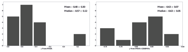
Figure 1: Distribution of $\gamma$ in eq. (2). Left: the distribution of $\gamma$ obtained from the fitting only to the MWA data. Right: same as Left panel but also with a 1500 MHz flux density.

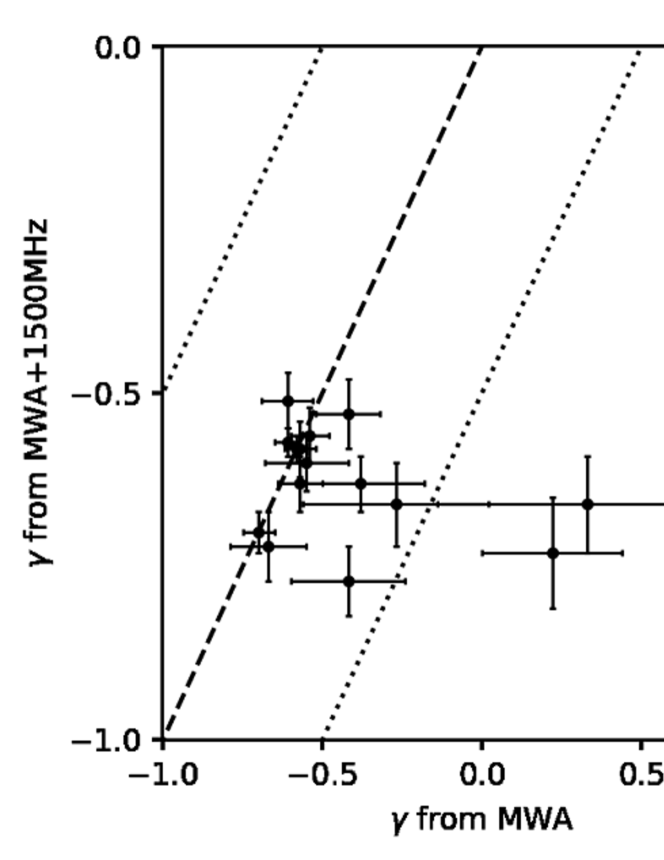
Figure 2: Comparison between $\gamma$ obtained from MWA data with and without 1500 MHz flux density. The errors are from Table 2. Dashed line represents the 1 to 1 diagonal, and dotted lines are the envelope obtained by shifting the diagonal by a factor 0.5 along the abscissa and ordinate.

We first present the distribution of estimated $\gamma$ in Figure 1. The left panel shows the $\gamma$ distribution from the fitting obtained solely with MWA data, and the right panel is with MWA and $1500\;[\mbox{MHz}]$ data combined. We show the mean and median with the standard and quantile deviation in both panels. We note that three galaxies in our sample (HRS 122, 163 and 204) are fitted only including MWA flux densities due to the low signal-to-noise of available $1500\,\;[\mbox{MHz}]$ detections (Boselli et al., 2015). We clearly see that two galaxies (HRS 25 and 144) are outliers in the left panel of Fig. 1, while they do not show any deviation from the bulk of the population when the shorter frequency data are included. We note that the origins of the radio continuum measurement are the same (Condon et al., 1990) for all but one galaxy (HRS 306: Condon et al., 2002). Thus, this can hardly be a source of a systematic error, and indeed the estimated $\gamma$ of HRS 306 is consistent with others within the quoted measurement uncertainty.

In order to examine these outliers, we compare $\gamma$ only from the MWA data and both from MWA and 1500 MHz data on individual basis in Fig. 2. The two outliers are prominent in Fig. 2. We also see that the estimated slopes become $\gamma<-0.5$ for all the samples, even if some of them had a flatter $\gamma$ when estimated only from MWA data. This suggests that there is a critical frequency where the turnover appears between MWA frequencies and $1500\;[\mbox{MHz}]$. At low frequencies, the spectral slope is prone to be flatter due to the free-free absorption (e.g., Calistro Rivera et al., 2017; Schober et al., 2017; Chyży et al., 2018). In addition, Schober et al. (2017) show that a Milky Way-like galaxy (similar in SFR) has the critical frequency one order of magnitude lower than the MWA frequency. However, HRS 25 and 144 have a SFR similar to the Milky Way (Boselli et al., 2015) and a critical frequency between MWA frequencies and $1500\;[\mbox{MHz}]$. This would be difficult to explain by the conjecture of Schober et al. (2017). Possible reasons for this are 1) poor statistics, i.e., fewer data can constrain the fitted slope only weakly, and 2) physical peculiarity of the galaxy. As for HRS 25 might really have a flatter slope, but very possibly it is due to the statistical uncertainty. In contrast, HRS 144 is identified as a Seyfert galaxy from the BPT diagram (e.g., Baldwin et al., 1981; Kewley et al., 2001; Kauffmann et al., 2003; Schawinski et al., 2007), and the galactic nuclei affects the spectral slope. Further, an Hi absorption towards the core of HRC 144 is reported from the VIVA observation (Chung et al., 2009). Hence, it would be natural that the radio continuum emission is not consistent with that of a purely star-forming galaxy. In this case, the shallow slope is physical. To have a firm conclusion for these two galaxies, we would need more data in a wide frequency range, e.g., from RACS (Hale et al., 2021). We leave this as our future work.

We adopt the averaged $\gamma$ obtained with the MWA frequencies and $1500\;[\mbox{MHz}]$ for the estimation of SFR in the following (Section 4.2). The fitting results are shown in Appendix B.

4.2 Star Formation Rate (SFR) from the low-frequency emission

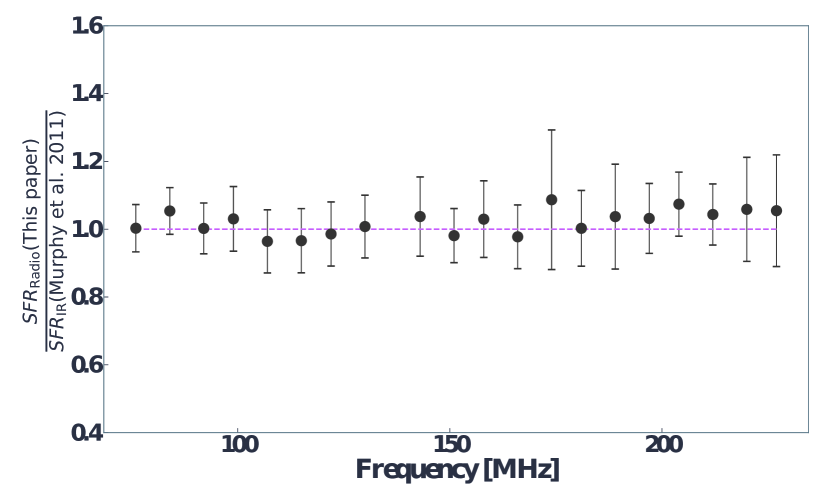
Figure 3: Comparison between $\mathrm{SFR}_{\mathrm{radio},\,\nu}$ and $\mathrm{SFR}_{\mathrm{IR}}$ at each MWA frequency. Symbols are the averages of $\mathrm{SFR}_{\mathrm{radio},\,\nu}$ among the sample galaxies, and the error bars represent the standard deviation in the sample. Upper panel shows the SFRs estimated with individually obtained $\gamma$ and $q_{1500\,[{\rm MHz}]}$ for the calibration of $\mathrm{SFR}_{\mathrm{radio},\,\nu}$. Middle panel is the same but with averaged $\gamma$ and $q_{1500\,[{\rm MHz}]}$. Bottom panel compares the SFR ratios from these two approaches.

Here we show the comparison between $\mathrm{SFR}_{\mathrm{radio},\,\nu}$ defined by eq. 3.2 with $\mathrm{SFR}_{\mathrm{IR}}$ (eq. 3), and ${\rm SFR}_{{\rm FUV}+{\rm 24}\mu{\rm m}}$ (Boselli et al., 2015) described as

$${\rm SFR}_{{\rm FUV}+{\rm 24}\mu{\rm m}}=6.21\times 10^{-44}\left(L_{\rm FUV,\,obs}+3.89L_{24\,\mu{\rm m}}\right)\;,$$ (6)

obtained from the calibration of Hao et al. (2011). Here the units of luminosities are measured by $[\mbox{erg\,s}^{-1}]$.

Figure 3 shows the ratio between $\mathrm{SFR}_{\mathrm{radio},\,\nu}$ and $\mathrm{SFR}_{\mathrm{IR}}$. We used the $q_{1500\,{\rm MHz}}$ and $\gamma$ of individual samples in eq. 3.2. Symbols are the averages of $\mathrm{SFR}_{\mathrm{radio},\,\nu}$ among the sample galaxies at each MWA frequency, and the error bars represent the standard deviation in the sample. Note that the number of galaxies at each frequency is different because we restricted to the sample with high $S/N$ for each flux densities ($S/N\geq 5$). The estimated $\mathrm{SFR}_{\mathrm{IR}}$s are consistent within a range of $\sim 10$ %.

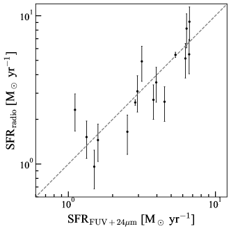
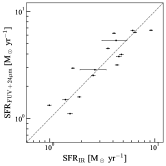
Figure 4: Comparison between ${\rm SFR}_{\rm IR}$, ${\rm SFR}_{{\rm FUV+}24\mu{\rm m}}$, and ${\rm SFR}_{\rm radio}$. Three panels show the comparison between ${\rm SFR}_{\rm IR}$ and ${\rm SFR}_{\rm radio}$, ${\rm SFR}_{{\rm FUV+}24\mu{\rm m}}$ and ${\rm SFR}_{\rm radio}$, and ${\rm SFR}_{\rm IR}$ and ${\rm SFR}_{{\rm FUV+}24\mu{\rm m}}$, from the top to the bottom.

We then examine the consistency of the radio SFR with other SFR indicators. We show the comparison between ${\rm SFR}_{\rm IR}$ and ${\rm SFR}_{\rm radio}$, ${\rm SFR}_{{\rm FUV+}24\mu{\rm m}}$ and ${\rm SFR}_{\rm radio}$, and ${\rm SFR}_{\rm IR}$ and ${\rm SFR}_{{\rm FUV+}24\mu{\rm m}}$, in Fig. 4. Here ${\rm SFR}_{\rm radio}$ stands for the radio SFR at 151 MHz, $\mathrm{SFR}_{\mathrm{radio},\,151\,{\rm MHz}}$. The top panel of Fig. 4 clearly indicates that the SFR estimated from the radio continuum is consistent and unbiased with respect to that from IR emission, by construction. We note that the scatter is not negligible (the scatter $\sigma^{2}=0.089$, and Pearson’s correlation coefficient is $\rho=0.77$). Note that the correlation analysis and linear regression in the following are performed in logarithmic scale. The scatter of the correlation is comparable to the typical measurement error of the radio side, and we may conclude that it is mainly caused by the observational error.

A similar comparison is presented in the middle panel of Fig. 4, for ${\rm SFR}_{{\rm FUV+}24\mu{\rm m}}$ and ${\rm SFR}_{\rm radio}$. Again the radio SFR estimator is consistent with the UV+24$\,\mu$m hybrid estimator of Hao et al. (2011) used in Boselli et al. (2015). We note that Boselli et al. (2015) did not provide the error on the UV+24$\,\mu$m estimates. The scatter is smaller than the top panel ($\sigma^{2}=0.064$ and the correlation coefficient is $\rho=0.87$). This can be explained as follows. The timescale of the UV continuum $t_{\rm UV}$ is longer than $t_{\rm OB}$. In contrast, the timescale of radio continuum $t_{\rm radio}$ is longer in general, $t_{\rm radio}\sim 10^{8}\;[\rm yr]$ (e.g., Condon, 1992), comparable to the radio continuum $t_{\rm UV}\sim 10^{8}\;[{\rm yr}]\simeq t_{\rm radio}$. Then, as far as the contribution of the visible star formation is significant (relatively low SFR, say ${\rm SFR}\lesssim 10\;[M_{\odot}\,\mbox{yr}^{-1}]$), the correlation is tight. Further, at ${\rm SFR}\simeq 10\;[M_{\odot}\,\mbox{yr}^{-1}]$, it is well known that the IR dominates the luminosity from star formation activity (e.g., Takeuchi et al., 2010, 2013). In addition, since the dust opacity becomes large at high SFR, the apparent dust continuum tends to be emitted at long wavelengths ($\lambda\gtrsim 60\;[\mu{\rm m}]$). Then, the mid-IR emission may not be strongly related to the SFR, and the 24-$\mu$m based hybrid SFR estimator tends to underestimate the SFR (e.g., Takeuchi et al., 2005b), resulting in the large deviation at high SFR in the middle panel in Fig. 4.

This effect is also visible in the bottom panel in Fig. 4. The scatter in the bottom panel is $\sigma^{2}=0.076$ and the correlation coefficient is $\rho=0.69$, not very tight. This might indicate the limitation of the MIR-based hybrid estimator. To summarize, the radio continuum SFR estimator works as an unbiased measure of the SFR, though we should keep in mind the nonnegligible scatter.

5 Discussion

We further compare our results in Section 4.1 with previous works. Extensive works have been published from LOFAR team.

5.1 Spectral index $\gamma$

First we examine the value of the spectral index $\gamma$. We obtained the average $\gamma=-0.63\pm 0.07$ with MWA and $1500\,\;[\mbox{MHz}]$ data, while Calistro Rivera et al. (2017) and Chyży et al. (2018) obtained $-0.78\pm 0.24$ and $-0.56\pm 0.11$, respectively. All are consistent with each other within the range of quoted errors. The slight difference is due to the different sample selection: while we used nearby galaxies within $25\;\mbox{Mpc}$, Calistro Rivera et al. (2017) used 758 galaxies up to $z\sim 2$, and Chyży et al. (2018) used 118 galaxies up to $z=0.04$. In turn, it would be interesting to examine the evolution of $\gamma$ with redshifts (e.g., Buat et al., 2011; Mao et al., 2011; Schleicher & Beck, 2013; Solarz et al., 2016; Delvecchio et al., 2021; Matthews et al., 2021). Chyży et al. (2018) claimed that the slope is steeper at higher frequencies ($1.3\mbox{--}5\;[\mbox{GHz}]$). Due to the redshift of SEDs, the slope of galaxy samples would appear to be steeper at higher-$z$ in the sample of Calistro Rivera et al. (2017), taken from $z\sim 2$.

5.2 Calibration of the radio SFR

We then compare our global calibration of the SFR with other works. In Section 4.2, we discussed the consistency of our SFR calibrations using the low-frequency emission. To calculate the radio SFR more accurately, we need the SED of each galaxy (Section 4.2). Since star-forming galaxies have a variety of $q_{\nu}$ at low frequencies ($\sim 0.53\;\mathrm{dex}$ in Figs. 14 and 15 of Calistro Rivera et al. 2017) and the physical details are still not fully understood, the radio SFR calibration would have some uncertainty. Substituting median values $\gamma=-0.63$, $q_{1500\,[{\rm MHz}]}=2.48$ and $\nu=150\,\;[{\rm MHz}]$ into eq. (3.2) yields the following equation:

$${\rm SFR}_{\rm radio,\,151\,{\rm MHz}}=$$

$$\quad\left(1.03\pm 0.27\right)\times 10^{-29}L_{\mathrm{radio},\,151\,{\rm MHz}}\,[\mathrm{erg}\,\mathrm{s}^{-1}]\;.$$ (7)

For example, Calistro Rivera et al. (2017) have obtained the coefficient of $0.76\pm 0.08$ at $z=0$ [their eq. (11)] from their calibration. Thus, we should keep in mind that the SFR calibration has this amount of uncertainty, possibly caused by the galaxy selection and the variation of $q_{\nu}$ at low frequencies.

Gürkan et al. (2018) investigated the relation between the low frequency radio luminosity obtained by LOFAR at 150 MHz and the SFR for galaxies at $0\lesssim z\lesssim 0.3$. They used the data in the Herschel Astrophysical Terahertz Large Area Survey (H-ATLAS: Eales et al. 2010) North Galactic Pole (NGP) field ($\sim 142\mbox{deg}^{2}$. The SFR was estimated from the SED of their sample by the SED fitting using MAGPHYS (da Cunha et al., 2008). They have made a classification of sample galaxies by the optical emission line diagnostics by the SDSS spectra. They adopted the equation

$$L_{\rm radio,150\,MHz}=L_{1}{\rm SFR}^{\beta}\;,$$ (8)

but used a logarithmic scale for the parameter estimation. They obtained $\beta=1.07\pm 0.01$, $L_{1}=10^{22.06\pm 0.01}\;[\mbox{W\, Hz}^{-1}]$, and $\sigma=1.45\pm 0.04$ for their star forming galaxies.

Wang et al. (2019) used the 150-MHz selected LOFAR value-added source catalogue in the Hobby–Eberly Telescope Dark Energy Experiment (HETDEX) Spring Field and cross-matched with the 60-$\mu$m selected Revised IRAS Faint Source Survey Redshift (RIFSC$z$) catalogue at $z\lesssim 0.05$. They have estimated $L_{\rm radio,150\,MHz}$ for the cross-matched sources and compared it with ${\rm H}\alpha$, $60\;\mu$m, and total IR-based SFR estimators. They obtained

$$\log L_{\rm radio,150\,MHz}$$

$$\quad=\left(1.35\pm 0.06\right)\log{\rm SFR}_{{\rm H}\alpha}+\left(3.20\pm 0.06\right)\;,$$ (9)

$$\log L_{\rm radio,150\,MHz}$$

$$\quad=\left(1.31\pm 0.05\right)\log{\rm SFR}_{60\mu{\rm m}}+\left(3.14\pm 0.06\right)\;,$$ (10)

$$\log L_{\rm radio,150\,MHz}$$

$$\quad=\left(1.37\pm 0.05\right)\log{\rm SFR}_{{\rm IR}}+\left(3.09\pm 0.05\right)\;.$$ (11)

Note that these estimates are for the subsample above their 90-% completeness limit, roughly corresponding to $\log{\rm SFR}\gtrsim 0.5$. If they use the whole sample, the slope is significantly flatter and close to unity.

More recently, Smith et al. (2021) presented the result of the LOFAR Surveys Key Science Project, with the 150 MHz data over the European Large Area Infrared Space Observatory Survey-North 1 field ($z\lesssim 1$). They obtained

$$\log L_{\rm radio,150\,MHz}$$

$$\quad=(22.221\pm 0.008)+(1.058\pm 0.007)\log{\rm SFR}\;.$$ (12)

They pointed out an upward deviation at lower-SFR regime toward higher redshifts. Bonato et al. (2021) performed LOFAR deep observations of the Lockman Hole field at 150MHz to examine the relation. They summarized the related results including above-mentioned works and found that most of them agree with each other within the range of sample scatter (see their Fig. 4). They also point out that putting the selection by statistical significance of the source would bias the relation.

All these results are expressed in the form of SFR–radio luminosity relation, rather than the reverse, which we believe is practical. Then, it is difficult to compare these relations with eq. (7). However, since most of them show a slope close to unity, it would still make sense to compare the relations by flipping SFR and $L_{\rm radio}$. By this indirect comparison, we safely conclude that our radio-luminosity SFR estimator is consistent with most of the preceding LOFAR-based works at $z\simeq 0$.

6 Summary

In this study, we examine the correlation between integrated low-frequency radio and infrared luminosities for a sample of 18 galaxies extracted from Herschel Reference Survey (HRS) catalog (Boselli et al., 2015). We use flux densities obtained by the Murchison Widefield Array (MWA) as a part of the GLEAM survey.

We focused on the radio-to-infrared (IR) correlation coefficient, $q_{\nu}$, and applied a model as

$$q_{\nu}=-\gamma\log{\nu}+\beta$$

[eq. (2)]. We found that $q_{\nu}$ from the MWA bands to $1500\,\;[\mbox{MHz}]$ can be well approximated this single power law model, and obtained the slope $\gamma$ consistent with previous studies (median $\gamma=-0.63$, $q_{1500\,{\rm MHz}}=2.48$).

We also investigated the consistency of the radio SFR estimator ${\rm SFR}_{\rm radio}$ expected to be an extinction-free indicator. The radio SFR estimator performs stably within the frequency range of MWA. It is consistent with the total IR estimator by construction, with a scatter due to the details of the star formation history. The advantage of ${\rm SFR}_{\rm radio}$ is that it does not require multifrequency observations for normal star-forming galaxies, unlike the total IR estimator.

For further understanding of the star formation activity as seen from low-frequency, we need a larger sample with multiband radio observations. Among such future projects, the updated GLEAM survey will be one of the most promising one to reveal physical details, with an order-of-magnitude better angular resolution and sensitivity than the latest survey. Data from RACS (Hale et al., 2021) will also help further investigation, but we leave this as our future work.

This work is based on the HRS data together with GLEAM survey maps, both of which are available from their data archive in public.

This work has been supported by the Japan Society for the Promotion of Science (JSPS) Grants-in-Aid for Scientific Research (19H05076 and 21H01128). This work has also been supported in part by the Sumitomo Foundation Fiscal 2018 Grant for Basic Science Research Projects (180923), and the Collaboration Funding of the Institute of Statistical Mathematics “New Development of the Studies on Galaxy Evolution with a Method of Data Science”. SC has been supported by the JSPS (21J23611). Parts of this research were conducted by the Australian Research Council Centre of Excellence for All Sky Astrophysics in 3 Dimensions (ASTRO 3D), through project number CE170100013.

Appendix A Galaxy images

Here we show the radio contours superposed on the SDSS $i$-band images of all the sample galaxies in Figure 5.

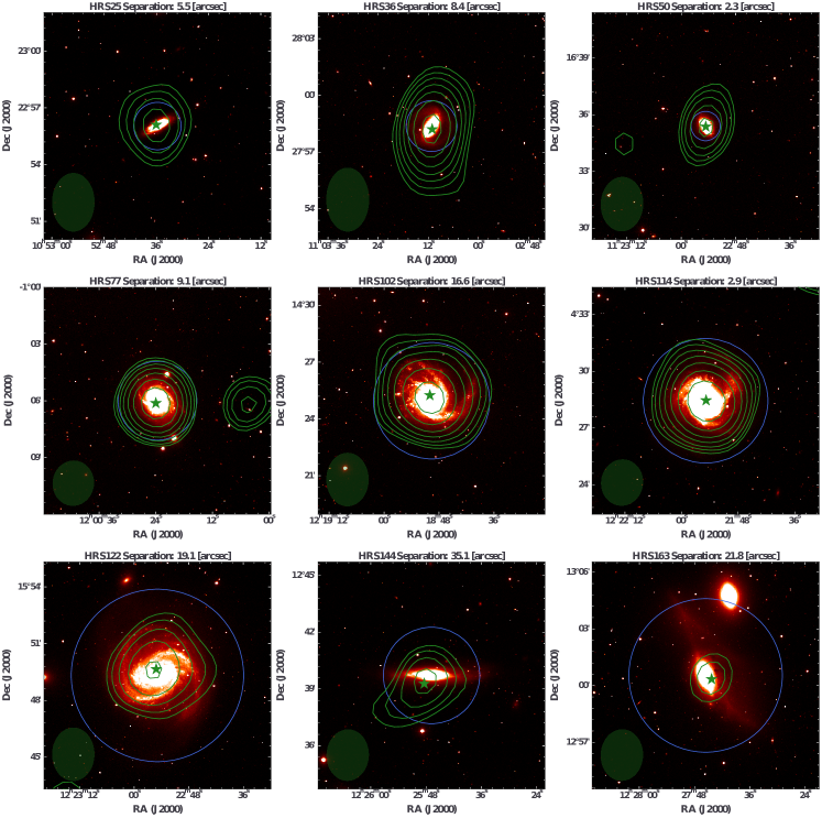
Figure 5: These are the SDSS (Abolfathi et al., 2018) i-band images with radio contours from the GLEAM survey at $170-231\;[\mbox{MHz}]$ (solid green lines). These galaxies are selected in Section 2. We draw the green contours started from the 3$\sigma$ local noise and increase by a factor of the square root of $2^{n}$ (“n” is an integer). The green star marker shows the location of a radio source referred to as the GLEAM catalog. The size of this marker does not mean any feature of observations. The blue circle shows the isophotal optical size at $25\,\mathrm{mag}\,\mathrm{arcsec}^{-2}$ from Boselli et al. (2010). On the bottom left in each plot, we show the beam size of the GLEAM survey.

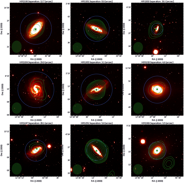
Figure 5: — Continued.

Appendix B Fitting results

The fitting results of the whole sample is presented in Figure 6.

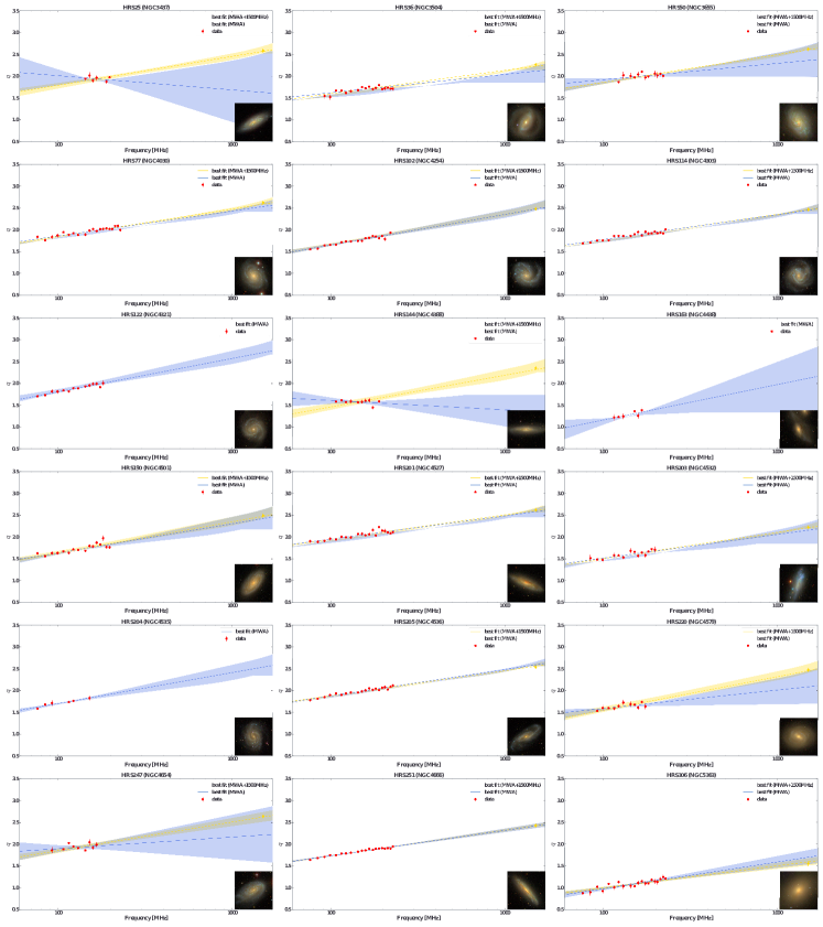
Figure 6: These figures show the fitting result. Red points show fluxes at each MWA frequency, and a yellow point shows the flux at $1500\;[\mbox{MHz}]$ (Boselli et al., 2015). Blue solid line shows the best fitting line, and the shaded region represents the 95% confidence interval for the fitting to MWA frequencies. Yellow line and shaded area show the fitting result with $1500\;[\mbox{MHz}]$ besides MWA frequencies (For HRS122, 163 and 204, we do not display these because of the lack of high-quality data at $1500\;[\mbox{MHz}]$ data). On the bottom right, we show the SDSS-RGB stacking image for each galaxy.

References

- Abolfathi et al. (2018) Abolfathi, B., Aguado, D. S., Aguilar, G., et al. 2018, ApJS, 235, 42
- Appleton et al. (2004) Appleton, P. N., Fadda, D. T., Marleau, F. R., et al. 2004, ApJS, 154, 147
- Baldwin et al. (1981) Baldwin, A., Phillips, M. M., & Terlevich, R. 1981, PASP, 93, 817
- Bell (2003) Bell, E. F. 2003, ApJ, 586, 794
- Bendo et al. (2012) Bendo, G. J., Galliano, F., & Madden, S. C. 2012, MNRAS, 423, 197
- Bicay & Helou (1990) Bicay, M. D., & Helou, G. 1990, ApJ, 362, 59
- Bonato et al. (2021) Bonato, M., Prandoni, I., De Zotti, G., et al. 2021, A&A, 656, A48
- Boselli et al. (2015) Boselli, A., Fossati, M., Gavazzi, G., et al. 2015, A&A, 579, A102
- Boselli et al. (2010) Boselli, A., Eales, S., Cortese, L., et al. 2010, PASP, 122, 261
- Bourne et al. (2011) Bourne, N., Dunne, L., Ivison, R. J., et al. 2011, MNRAS, 410, 1155
- Buat et al. (2011) Buat, V., Giovannoli, E., Takeuchi, T. T., et al. 2011, A&A, 529, A22
- Buat et al. (2007) Buat, V., Takeuchi, T. T., Iglesias-Páramo, J., et al. 2007, ApJS, 173, 404
- Calistro Rivera et al. (2017) Calistro Rivera, G., Williams, W. L., Hardcastle, M. J., et al. 2017, MNRAS, 469, 3468
- Chung et al. (2009) Chung, A., van Gorkom, J. H., Kenney, J. D. P., Crowl, H., & Vollmer, B. 2009, AJ, 138, 1741
- Chyży et al. (2018) Chyży, K. T., Jurusik, W., Piotrowska, J., et al. 2018, A&A, 619, A36
- Ciesla et al. (2012) Ciesla, L., Boselli, A., Smith, M. W. L., et al. 2012, A&A, 543, A161
- Ciesla et al. (2014) Ciesla, L., Boquien, M., Boselli, A., et al. 2014, A&A, 565, A128
- Condon (1992) Condon, J. J. 1992, ARA&A, 30, 575
- Condon et al. (1991) Condon, J. J., Anderson, M. L., & Helou, G. 1991, ApJ, 376, 95
- Condon et al. (2002) Condon, J. J., Cotton, W. D., & Broderick, J. J. 2002, AJ, 124, 675
- Condon et al. (1990) Condon, J. J., Helou, G., Sanders, D. B., & Soifer, B. T. 1990, ApJS, 73, 359
- Cortese et al. (2012) Cortese, L., Boissier, S., Boselli, A., et al. 2012, A&A, 544, A101
- Cortese et al. (2014) Cortese, L., Fritz, J., Bianchi, S., et al. 2014, MNRAS, 440, 942
- da Cunha et al. (2008) da Cunha, E., Charlot, S., & Elbaz, D. 2008, MNRAS, 388, 1595
- Delvecchio et al. (2021) Delvecchio, I., Daddi, E., Sargent, M. T., et al. 2021, A&A, 647, A123
- Devereux & Eales (1989) Devereux, N. A., & Eales, S. A. 1989, ApJ, 340, 708
- Eales et al. (2010) Eales, S., Dunne, L., Clements, D., et al. 2010, PASP, 122, 499
- Galametz et al. (2013) Galametz, M., Kennicutt, R. C., Calzetti, D., et al. 2013, MNRAS, 431, 1956
- Gürkan et al. (2018) Gürkan, G., Hardcastle, M. J., Smith, D. J. B., et al. 2018, MNRAS, 475, 3010
- Haarsma et al. (2000) Haarsma, D. B., Partridge, R. B., Windhorst, R. A., & Richards, E. A. 2000, ApJ, 544, 641
- Hale et al. (2021) Hale, C. L., McConnell, D., Thomson, A. J. M., et al. 2021, PASA, 38, e058
- Hao et al. (2011) Hao, C.-N., Kennicutt, R. C., Johnson, B. D., et al. 2011, ApJ, 741, 124
- Helou et al. (1985) Helou, G., Soifer, B. T., & Rowan-Robinson, M. 1985, ApJ, 298, L7
- Hummel (1986) Hummel, E. 1986, A&A, 160, L4
- Hurley-Walker et al. (2017) Hurley-Walker, N., Callingham, J. R., Hancock, P. J., et al. 2017, MNRAS, 464, 1146
- Jarvis et al. (2010) Jarvis, M. J., Smith, D. J. B., Bonfield, D. G., et al. 2010, MNRAS, 409, 92
- Kauffmann et al. (2003) Kauffmann, G., Heckman, T. M., Tremonti, C., et al. 2003, MNRAS, 346, 1055
- Kennicutt (1983) Kennicutt, R. C. 1983, ApJ, 272, 54
- Kennicutt (1998) Kennicutt, R. C. 1998, ARA&A, 36, 189
- Kennicutt et al. (2009) Kennicutt, R. C., Hao, C. N., Calzetti, D., et al. 2009, Astrophysical Journal, 703, 1672
- Kewley et al. (2001) Kewley, L. J., Dopita, M. A., Sutherland, R. S., Heisler, C. A., & Trevena, J. 2001, ApJ, 556, 121
- Kroupa (2002) Kroupa, P. 2002, Science, 295, 82
- Mao et al. (2011) Mao, M. Y., Huynh, M. T., Norris, R. P., et al. 2011, ApJ, 731, 79
- Matthews et al. (2021) Matthews, A. M., Condon, J. J., Cotton, W. D., & Mauch, T. 2021, ApJ, 914, 126
- Molnár et al. (2021) Molnár, D. C., Sargent, M. T., Leslie, S., et al. 2021, MNRAS, 504, 118
- Murphy et al. (2015) Murphy, E., Sargent, M., Beswick, R., et al. 2015, in Advancing Astrophysics with the Square Kilometre Array (AASKA14), 85
- Murphy et al. (2006) Murphy, E. J., Braun, R., Helou, G., et al. 2006, ApJ, 638, 157
- Murphy et al. (2011) Murphy, E. J., Condon, J. J., Schinnerer, E., et al. 2011, ApJ, 737, 67
- Pepiak et al. (2014) Pepiak, A., Pollo, A., Takeuchi, T. T., Solarz, A., & Jurusik, W. 2014, Planet. Space Sci., 100, 12
- Pierini et al. (2003) Pierini, D., Popescu, C. C., Tuffs, R. J., & Völk, H. J. 2003, A&A, 409, 907
- Read et al. (2018) Read, S. C., Smith, D. J. B., Gürkan, G., et al. 2018, MNRAS, 480, 5625
- Schawinski et al. (2007) Schawinski, K., Thomas, D., Sarzi, M., et al. 2007, MNRAS, 382, 1415
- Schleicher & Beck (2013) Schleicher, D. R. G., & Beck, R. 2013, A&A, 556, A142
- Schober et al. (2016) Schober, J., Schleicher, D. R. G., & Klessen, R. S. 2016, ApJ, 827, 109
- Schober et al. (2017) Schober, J., Schleicher, D. R. G., & Klessen, R. S. 2017, MNRAS, 468, 946
- Shao et al. (2018) Shao, L., Koribalski, B. S., Wang, J., Ho, L. C., & Staveley-Smith, L. 2018, MNRAS, 479, 3509
- Smith et al. (2014) Smith, D. J. B., Jarvis, M. J., Hardcastle, M. J., et al. 2014, MNRAS, 445, 2232
- Smith et al. (2021) Smith, D. J. B., Haskell, P., Gürkan, G., et al. 2021, A&A, 648, A6
- Solarz et al. (2019) Solarz, A., Pollo, A., Bilicki, M., et al. 2019, PASJ, 71, 28
- Solarz et al. (2016) Solarz, A., Takeuchi, T. T., & Pollo, A. 2016, A&A, 592, A155
- Takeuchi et al. (2005a) Takeuchi, T. T., Buat, V., & Burgarella, D. 2005a, A&A, 440, L17
- Takeuchi et al. (2010) Takeuchi, T. T., Buat, V., Heinis, S., et al. 2010, A&A, 514, A4
- Takeuchi et al. (2005b) Takeuchi, T. T., Buat, V., Iglesias-Páramo, J., Boselli, A., & Burgarella, D. 2005b, A&A, 432, 423
- Takeuchi et al. (2016) Takeuchi, T. T., Morokuma-Matsui, K., Iono, D., et al. 2016, SKA Japan Science Book 2016, arXiv:1603.01938
- Takeuchi et al. (2013) Takeuchi, T. T., Sakurai, A., Yuan, F.-T., Buat, V., & Burgarella, D. 2013, Earth, Planets, and Space, 65, 281
- Tingay et al. (2013) Tingay, S. J., Oberoi, D., Cairns, I., et al. 2013, Journal of Physics: Conference Series, 440, 012033
- Tisanić et al. (2022) Tisanić, K., De Zotti, G., Amiri, A., et al. 2022, A&A, 658, A21
- Wang et al. (2019) Wang, L., Gao, F., Duncan, K. J., et al. 2019, A&A, 109, 1
- Wang et al. (2019) Wang, L., Gao, F., Duncan, K. J., et al. 2019, A&A, 631, A109
- Wayth et al. (2015) Wayth, R. B., Lenc, E., Bell, M. E., et al. 2015, PASA, 32, e025
- Yun et al. (2001) Yun, M. S., Reddy, N. A., & Condon, J. J. 2001, ApJ, 554, 803