Online Convolutional Re-parameterization

Abstract

Structural re-parameterization has drawn increasing attention in various computer vision tasks. It aims at improving the performance of deep models without introducing any inference-time cost. Though efficient during inference, such models rely heavily on the complicated training-time blocks to achieve high accuracy, leading to large extra training cost. In this paper, we present online convolutional re-parameterization (OREPA), a two-stage pipeline, aiming to reduce the huge training overhead by squeezing the complex training-time block into a single convolution. To achieve this goal, we introduce a linear scaling layer for better optimizing the online blocks. Assisted with the reduced training cost, we also explore some more effective re-param components. Compared with the state-of-the-art re-param models, OREPA is able to save the training-time memory cost by about 70% and accelerate the training speed by around 2$\times$. Meanwhile, equipped with OREPA, the models outperform previous methods on ImageNet by up to +0.6%. We also conduct experiments on object detection and semantic segmentation and show consistent improvements on the downstream tasks. Codes are available at https://github.com/JUGGHM/OREPA_CVPR2022.

1 Introduction

Convolutional Neural Networks (CNNs) have seen the success of many computer vision tasks, including classification [21, 27, 38, 25], object detection [33, 28, 32], segmentation [7, 44], . The trade-off between accuracy and model efficiency has been widely discussed. In general, a model with higher accuracy usually requires a more complicated block [25, 24, 18], a wider or deeper structure [41, 4]. However, such models are always too heavy to be deployed, especially in the scenarios where the hardware performance is limited, and real-time inference is required. Taking efficiency into consideration, smaller, compacter, and faster models are preferred.

In order to obtain a deploy-friendly model and keep a high accuracy, structural re-parameterization based methods [14, 16, 17, 19] are proposed for a “free” performance improvement. In such methods, the models have different structures during the training phase and the inference phase. Specifically, they [16, 1] use complicated training-phase topologies, , re-parameterized blocks, to improve the performance. After training, they squeeze a complicated block into a single linear layer through equivalent transformation. The squeezed models are usually with a neat architecture, , usually a VGG-like [17] or a ResNet-like [16] structure. From this perspective, the re-parameterization strategies can improve model performances without introducing additional inference-time cost.

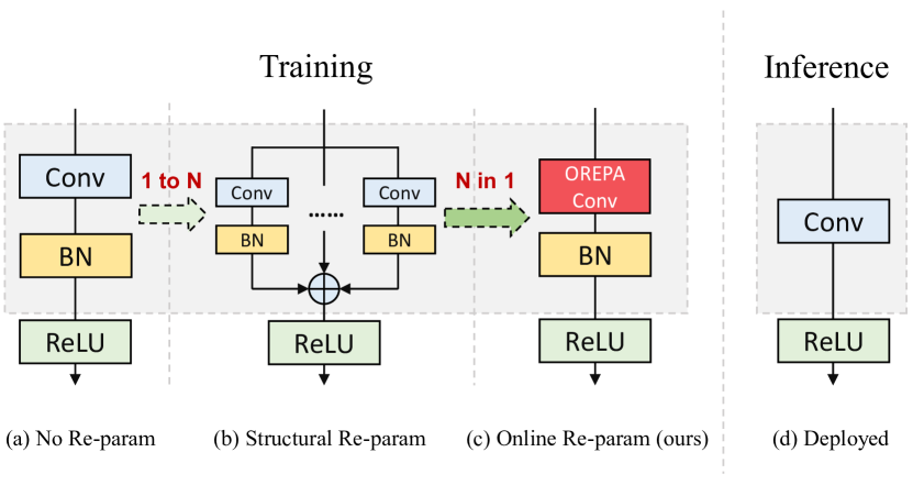
Figure 1: Comparison of (a) a vanilla convolutional layer, (b) a typical re-param block, and (c) our online re-param block in the training phase. All of these structures are converted to the same (d) inference-time structure.

It is believed that the normalization (norm) layer is the crucial component in re-param models. In a re-param block (fig:intro(b)), a norm layer is always added right-after each computational layer. It is observed that the removal of such norm layers would lead to severe performance degradation [17, 16]. However, when considering the efficiency, the utilization of such norm layers unexpectedly brings huge computational overhead in the training phase. The complicated block could be squeezed into a single convolutional layer in the inference phase. But, during training, the norm layers are non-linear, , they divide the feature map by its standard deviation, which prevents us from merging the whole block. As a result, there exist plenty of intermediate computational operations (large FLOPS) and buffered feature maps (high memory usage). Even worse, the high training budget makes it difficult to explore more complex and potentially stronger re-param blocks. Naturally, the following question arises,

• Why does normalization matter in re-param?

According to the analysis and experiments, we claim that it is the scaling factors in the norm layers that counts most, since they are able to diversify the optimization direction of different branches.

Based on the observations, we propose Online Re-Parameterization (OREPA) (fig:intro(c)), a two-stage pipeline which enables us to simplify the complicated training-time re-param blocks. In the first stage, block linearization, we remove all the non-linear norm layers and introduce the linear scaling layers. Such layers are with similar property as norm layers, that they diversify the optimization of different branches. Besides, these layers are linear, and can be merged into convolutional layers during training. The second stage, named block squeezing, simplifies the complicated linear block into a single convolutional layer. The OREPA significantly shrinks the training cost by reducing the computational and storage overhead caused by the intermediate computational layers, with only minor compromising on performance. Moreover, the high-efficiency makes it feasible to explore much more complicated re-parameterized topologies. To validate this, we further propose several re-parameterized components for better performance.

We evaluate the proposed OREPA on the ImageNet [13] classification task. Compared with the state-of-the-art re-param models [16], OREPA reduces the extra training-time GPU memory cost by 65$\%$ to 75$\%$, and speeds up the training process by 1.5$\times$ to 2.3$\times$. Meanwhile, our OREPA-ResNet and OREPA-VGG consistently outperform previous methods [16, 17] by +0.2%$\sim$+0.6%. We evaluate OREPA on the downstream tasks, , object detection and semantic segmentation. We find that OREPA could consistently bring performance gain on these tasks.

Our contributions can be summarized as follows:

• We propose the Online Convolutional Reparameterization (OREPA) strategy, which greatly improves the training efficiency of re-parameterization models and makes it possible to explore stronger re-param blocks.

• According to our analysis on the mechanism by which the re-param models work, we replace the norm layers with the introduced linear scaling layers, which still provides diverse optimization directions and preserves the representational capacity.

• Experiments on various vision tasks demonstrate OREPA outperforms previous re-param models in terms of both accuracy and training efficiency.

2 Related Works

2.1 Structural Re-parameterization

Structural re-parameterization [16, 17] is recently attached greater importance and utilized in lots of computer vision tasks, such as compact model design [18], architecture search [9, 43], and pruning [15]. Re-parameterization means different architectures can be mutually converted through equivalent transformation of parameters. For example, a branch of 1$\times$1 convolution and a branch of 3$\times$3 convolution, can be transferred into a single branch of 3$\times$3 convolution [17]. In the training phase, multi-branch [14, 16, 17] and multi-layer [19, 5] topologies are designed to replace the vanilla linear layers (conv or full connected layer [1]) for augmenting models. Cao et al.[5] have discussed how to merge a depthwise separable convolution kernel during training. Afterwards during inference, the training-time complex models are transferred to simple ones for faster inference. While benefiting from complex training-time topologies, current re-parameterization methods[14, 16, 19] are trained with non-negligible extra computational cost. When the block becomes more complicated for stronger representation, the GPU memory utilization and time for training will grow larger and longer, finally towards unacceptable. Different from previous re-param methods, we focus more on the training cost. We propose a general online convolutional re-parameterization strategy, which make the training-time structural re-parameterization possible.

2.2 Normalization

Normalization [26, 40, 2, 35] is proposed to alleviate the gradient vanishing problem when training very deep neural networks. It is believed that norm layers are very essential [36] as they smooth the loss landscape. Recent works on norm-free neural networks claim that norm layers are not indispensable [42, 37]. Through good initialization and proper regularization, normalization layers can be removed [42, 12, 37, 3] elegantly.

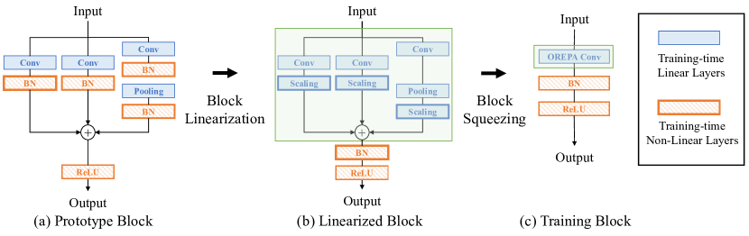
Figure 2: An overview of the proposed Online Re-Parameterization (OREPA), a two-stage pipeline. In the first stage (Block Linearization), we remove all the non-linear components in the prototype re-param block. In the second stage (Block Squeezing), we merge the block to a single convolutional layer (OREPA Conv). Through the steps, we significantly reduce the training cost while keep the high performance.

For the re-parameterization models, it is believed that norm layers in re-parameterized blocks are crucial [16, 17]. The norm-free variants would suffer from performance degradation. However, the training-time norm layers are non-linear, , they divide the feature map by its standard deviation, which prevents us from merging the blocks online. To make it feasible to perform online re-parameterization, we remove all the norm layers in re-param blocks, In addition, we introduce the linear alternative of norm layers, , the linear scaling layers.

2.3 Convolutional Decomposition

Standard convolutional layers are computational dense, leading to large FLOPs and parameter numbers. Therefore, convolutional decomposition methods [30, 39, 34] are proposed and widely applied in light-weighted models for mobile devices [23, 10]. Re-parameterization methods [14, 16, 19, 5, 9, 43] could be regarded as a certain form of convolutional decomposition as well, but towards more complicated topologies. The difference of our methods is that we decompose convolution at the kernel level rather than structure level.

3 Online Re-Parameterization

In this section, we introduce the proposed Online Convolutional Re-Parameterization. First, we analyze the key components, , the normalization layers in re-parameterization models, as preliminaries in sec:prelim. Based on the analysis, we propose the Online Re-Parameterization (OREPA), aiming to greatly reduce the training-time budgets of re-parameterization models. OREPA is able to simplify the complicated training-time block into a single convolutional layer and preserve the high accuracy. The overall pipeline of OREPA is illustrated in fig:orepa, which consists of a Block Linearization stage (sec:linearization) and a Block Squeezing stage (sec:trans). Next, in  sec:principle, we dig deeper into the effectiveness of re-parameterization by analyzing the optimization diversity of the multi-layer and multi-branch structures, and prove that both the proposed linear scaling layers and normalization layers have the similar effect. Finally, with the reduced training budget, we further explore some more components for a stronger re-parameterization (sec:components), with marginally increased cost.

3.1 Preliminaries: Normalization in Re-param

Table 1: Effectiveness of normalization layers in re-param models. To stabilize the training process, when removing the branch-wise norm layers, we add a post-addtion norm layer.

Variants	DBB-18	RepVGG-A0
Original	71.77	72.41
W/o branch-wise norm	71.35	71.15
W/o re-param	71.21	71.17

It is believed that the intermediate normalization layers are the key components for the multi-layer and multi-branch structures in re-parameterization. Taking the SoTA models, , DBB [16] and RepVGG [17] as examples, the removal of such layers would cause severe performance degradation, as shown in tab:norm. Such an observation is also experimentally supported by Ding et al.[16, 17]. Thus, we claim that the intermediate normalization layers are essential for performances of re-parameterization models.

However, the utilization of intermediate norm layers unexpectedly brings higher training budgets. We notice that in the inference phase, all the intermediate operations in the re-parameterization block are linear, thus can be merged into one convolutional layer, resulting in a simple structure. But during training, the norm layers are non-linear, , they divide the feature map by its standard deviation. As a result, the intermediate operations should be calculated separately, which leads to higher computational and memory costs. Even worse, such high cost would prevent the community from exploring stronger training blocks.

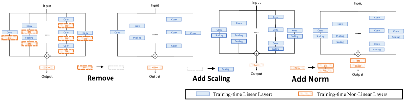
Figure 3: Three steps of block linearization. i) We first remove all the training-time non-linear normalization layers in the ra-param block. ii) Second, we add a linear scaling layer at the end of each branch to diversify the optimization directions. iii) Last, we add a post-normalization layer right after each block to stabilize training.

3.2 Block Linearization

As stated in sec:prelim, the intermediate normalization layers prevent us from merging the separate layers during training. However, it is non-trivial to directly remove them due to the performance issue. To tackle this dilemma, we introduce the channel-wise linear scaling operation as a linear alternative of normalization. The scaling layer contains a learnable vector, which scales the feature map in the channel dimension. The linear scaling layers have the similar effect as normalization layers, that they both encourage the multi-branches to be optimized towards diverse directions, which is the key to the performance improvement in re-parameterization. The detailed analysis of the effect is discussed in sec:principle. In addition to the effects on performance, the linear scaling layers could be merged during the training, making the online re-parameterization possible.

Based on the linear scaling layers, we modify the re-parameterization blocks as illustrated in fig:linearization. Specifically, the block linearization stage consists of the following three steps. First, we remove all the non-linear layers, , normalization layers in the re-parameterization blocks. Second, in order to maintain the optimization diversity, we add a scaling layer, the linear alternative of normalization, at the end of each branch. Finally, to stabilize the training process, we add a post-addition normalization layer right after the addition of all the branches.

Once finishing the linearization stage, there exist only linear layers in the re-param blocks, meaning that we can merge all the components in the block during the training phase. Next, we describe how to squeeze such a block into a single convolution kernel.

3.3 Block Squeezing

Benefiting from block linearization (sec:linearization), we obtain a linear block. In this section, we describe the standard procedure for squeezing a training-time linear block into a single convolution kernel. The block squeezing step converts the operations on intermediate feature maps, which are computation and memory expensive, into operations on kernels that are much more economic. This implies that we reduce the extra training cost of re-param from $O(H\times W)$ to $O(K_{H}\times K_{W})$ in terms of both computation and memory, where $(H,W),\ (K_{H},K_{W})$ are the spatial shapes of the feature map and the convolutional kernel.

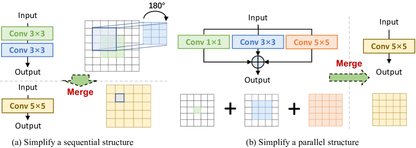
Figure 4: Simplification of sequential and parallel structures. Such simplifications convert the heavy computations on the feature maps to the lighter ones on the convolutional kernels.

In general, no matter how complicated a linear re-param block is, the following two properties always hold.

• All the linear layer in the block, , depth-wise convolution, average pooling, and the proposed linear scaling, can be represented by a degraded convolutional layer with a corresponding set of parameters. Please refer to the supplementary materials for details.

• The block can be represented by a series of parallel branches, each of which consists a sequence of convolutional layers.

With the above two properties, we can squeeze a block if we can simplify both i) a multi-layer (, the sequential structure) and ii) a multi-branch (, the parallel structure) into a single convolution. In the following part, we show how to simplify the sequential structure (fig:squeeze(a)) and the parallel structure (fig:squeeze(b)).

We first define the notations of convolution. Let $C_{i}$, $C_{o}$ denote the input and output channel numbers of a $K_{H}\times K_{W}$ sized 2d convolution kernel. $\mathbf{X}\in\mathbb{R}^{C_{i}\times H\times W}$, $\mathbf{Y}\in\mathbb{R}^{C_{o}\times H^{\prime}\times W^{\prime}}$ denote the input and output tensors. We omit the bias here as a common practice, the convolution process is denoted by

$$\mathbf{Y}=\mathbf{W}\ast\mathbf{X}.$$ (1)

Simplify a sequential structure.

Consider a stack of convolutional layers denoted by

$$\mathbf{Y}=\mathbf{W}_{N}(\mathbf{W}_{N-1}\ast\cdots(\mathbf{W}_{2}\ast(\mathbf{W}_{1}\ast\mathbf{X}))),$$ (2)

where $\mathbf{W}_{j}\in\mathbb{R}^{C_{j}\times C_{j-1}\times K_{H_{j}}\times K_{W_{j}}}$ satisfies $C_{0}=C_{i},\;C_{N}=C_{o}$. According to the associative law, such layers can be squeezed into one by convolving the kernels first according to Eq. (3).

$$\begin{split}\mathbf{Y}&=(\mathbf{W}_{N}(\mathbf{W}_{N-1}\ast\cdots(\mathbf{W}_{2}\ast\mathbf{W}_{1}))\ast\mathbf{X}\\ &=\mathbf{W}_{e}\ast\mathbf{X},\end{split}$$ (3)

where $\mathbf{W}_{j}$ is the weight of the $j^{th}$ layer. $\mathbf{W}_{e}$ denotes the end-to-end mapping matrix. The pixel-wise form of Eq. (3) is shown in the supplementary materials.

Simplify a parallel structure.

The simplification of a parallel structure is trivial. According to the linearity of convolution, we can merge multiple branches into one according to Eq. (4).

$$\mathbf{Y}=\sum_{m=0}^{M-1}(\mathbf{W}_{m}\ast\mathbf{X})=(\sum_{m=0}^{M-1}\mathbf{W}_{m})\ast\mathbf{X},$$ (4)

where $\mathbf{W}_{m}$ is the weight of the $m^{th}$ branch, and $(\sum_{m=0}^{M-1}\mathbf{W}_{m})$ is the unified weight. It is worth noting that when merging kernels with different sizes, we need to align the spatial centers of different kernels, , an 1$\times$1 kernel should be aligned with the center of a 3$\times$3 kernel.

Training overhead: from features to kernels.

No matter how complex the block is, it must be constituted by no more than multi-branch and multi-layer sub-topologies. Thus, it can be simplified into a single one according to the two simplification rules above. Finally, we could get the all-in-one end-to-end mapping weight and only convolve once during training. According to Eq. (3) and Eq. (4), we actually convert the operations (convolution, addition) on intermediate feature maps into those on convolutional kernels. As a result, we reduce the extra training cost of a re-param block from $O(H\times W)$ to $O(K_{H}\times K_{W})$.

3.4 Gradient Analysis on Multi-branch Topology

To understand why the block linearization step is feasible, why the scaling layers are important, we conduct analysis on the optimization of the unified weight re-parameterized. Our conclusion is that for the branches with norm layers removed, the utilization of scaling layers could diversify their optimization directions, and prevent them from degrading into a single one.

To simplify the notation, we take only single dimension of the output $\mathbf{Y}$. Consider a conv-scaling sequence (a simplified version of conv-norm sequence):

$$\Phi^{Conv-Scale}:=\{\mathbf{y}=\gamma\mathbf{W}\mathbf{x}|W\in\mathbb{R}^{o,i},\gamma\in\mathbb{R}^{o}\},$$ (5)

where $I=C_{i}\times K_{H}\times K_{W}$, $\mathbf{x}\in\mathbb{R}^{I}$ is vectorized pixels inside a sliding window, $y\in\mathbb{R}^{O}$, $O=1$, $\mathbf{W}$ is a convolutional kernel corresponding to certain output channel, and $\gamma$ is the scaling factor. Suppose all parameters are updated by stochastic gradient descent, the mapping $\mathbf{W}_{cs}:=\gamma\mathbf{W}$ is updated by:

$$\begin{split}&\mathbf{W}^{(t+1)}_{cs}:=\gamma^{(t+1)}\mathbf{W}^{(t+1)}\\ &=(\gamma^{(t)}-\eta\mathbf{W}^{(t)}\mathbf{x}^{\top}\frac{\partial L}{\partial\mathbf{y}})(\mathbf{W}^{(t)}-\eta\gamma^{(t)}\mathbf{x}^{\top}\frac{\partial L}{\partial\mathbf{y}})\\ &=\mathbf{W}^{(t)}_{cs}-\eta(vec(diag(\mathbf{W}^{(t)})^{2})+\left\|\gamma^{(t)}\right\|_{2}^{2})\mathbf{x}^{\top}\frac{\partial L}{\partial\mathbf{y}}\end{split}$$ (6)

where $L$ is the loss function of the entire model and $\eta$ is the learning rate. For a multi-branch topology with a shared $\gamma$, :

$$\Phi^{Conv-Scale}_{M}:=\{\mathbf{y}=\gamma\sum_{j=1}^{M}\mathbf{W}_{j}\mathbf{x}|\mathbf{W}_{j}\in\mathbb{R}^{o,i},\gamma\in\mathbb{R}^{o}\},$$ (7)

the end-to-end weight $\mathbf{W}_{e_{1},cs}:=\gamma\sum_{j=1}^{M}\mathbf{W}_{j}$ is optimized equally from that of Eq. (6):

$$\mathbf{W}^{(t+1)}_{e_{1},cs}-\mathbf{W}^{(t)}_{e_{1},cs}=\mathbf{W}^{(t+1)}_{cs}-\mathbf{W}^{(t)}_{cs},$$ (8)

with the same forwarding $t^{th}$-moment end-to-end matrix $\mathbf{W}^{(t)}_{cs}=\mathbf{W}^{(t)}_{e_{1},cs}$. Hence, $\Phi^{Conv-Scale}_{M}$ introduces no optimization change. This conclusion is also supported experimentally [16]. On the contrary, a multi-branch topology with branch-wise $\gamma$ provide such changes, :

$$\Phi^{Conv-Scale}_{M,2}:=\{\mathbf{y}=\sum_{j=1}^{M}\gamma_{j}\mathbf{W}_{j}\mathbf{x}|\mathbf{W}_{j}\in\mathbb{R}^{o,i},\gamma_{j}\in\mathbb{R}^{o}\}.$$ (9)

The end-to-end weight $\mathbf{W}_{e_{2},cs}:=\sum_{j=1}^{M}\gamma_{j}\mathbf{W}_{j}$ is updated differently from that of Eq. (6):

$$\mathbf{W}^{(t+1)}_{e_{2},cs}-\mathbf{W}^{(t)}_{e_{2},cs}\neq\mathbf{W}^{(t+1)}_{cs}-\mathbf{W}^{(t)}_{cs},$$ (10)

with the same precondition $\mathbf{W}^{(t)}_{cs}=\mathbf{W}^{(t)}_{e_{2},cs}$ and Condition 1 satisfied:

Condition 1

At least two of all the branches are active.

$$\begin{split}\exists\;&\mathbf{S}\subseteq\{1,2,\cdots,M\},\left|\mathbf{S}\right|\geq 2,\\ &such\;that\;\forall j\in\mathbf{S},\;vec(diag(\mathbf{W}_{j}^{(t)})^{2})+\left\|\gamma_{j}^{(t)}\right\|_{2}^{2}\neq\mathbf{0}\end{split}$$ (11)

Condition 2

The initial state of each active branch is different from that of each other.

$$\forall j_{1},j_{2}\in\mathbf{S},\;j_{1}\neq j_{2},\quad\mathbf{W}_{j_{1}}^{(0)}\neq\mathbf{W}_{j_{2}}^{(0)}.$$ (12)

Meanwhile, when Condition 2 is met, the multi-branch structure will not degrade into single one for both forwarding and backwarding. This reveals the following proposition explaining why the scaling factors are important. Note that both Condition 1 and 2 are always met when weights $\mathbf{W}_{j}^{(0)}$ of each branch is random initialized [20] and scaling factors $\gamma_{j}^{(0)}$ are initialized to 1.

Proposition 1

A single-branch linear mapping, when re-parameterizing parts or all of it by over-two-layer multi-branch topologies, the entire end-to-end weight matrix will be differently optimized. If one layer of the mapping is re-parameterized to up-to-one-layer multi-branch topologies, the optimization will remain unchanged.

So far, we have extended the discussion on how re-parameterization impacts optimization, from multi-layer only [1] to multi-branch included as well. Actually, all current effective re-parameterization topology [14, 16, 17, 19, 5] can be validated by either [1] or Proposition 1. For detailed derivation and discussion about this subsection, please refer to supplementary materials.

3.5 Block Design

Since the proposed OREPA saves the training cost by a large margin, it enables us to explore more complicated training blocks. Hereby, We design a novel of re-parameterization models, , OREPA-ResNet, by linearizing the state-of-the-art model DBB [16], and inserting the following components (fig:components).

Frequency prior filter.

In previous work [16], pooling layers are utilized in the block. According to Qin et al. [31], the pooling layer is a special case of the frequency filters. To this end, we add a Conv1$\times$1 - Frequency Filter branch.

Linear depthwise separable convolution. [5]

We slightly modify the depthwise separable convolution [10] by removing the intermediate non-linear activation layer, making it feasible to be merged during training.

Re-parameterization for 1$\times$1 convolution.

Previous works mainly focus on the Re-parameter for 3$\times$3 convolutional layers but ignore the 1$\times$1 ones. We propose to re-parameterize 1$\times$1 layers because they play an important role in the bottleneck structures [21, 4]. Specifically, we add an additional Conv1$\times$1 - Conv1$\times$1 branch.

Linear deep stem.

Large convolutional kernels are usually placed in the very beginning layers, , 7$\times$7 stem layers [21], aiming at achieving a larger receptive field. Guo et al.replace the 7$\times$7 conv layer with stacked 3$\times$3 layers for a higher accuracy [19]. However, the stacked convs at the very beginning layers require larger computational overhead due to the high-resolution. Note that we can squeeze the stacked deep stem with our proposed linear scaling layers to a 7$\times$7 conv layer, which can greatly reduce the training cost while keep the high accuracy.

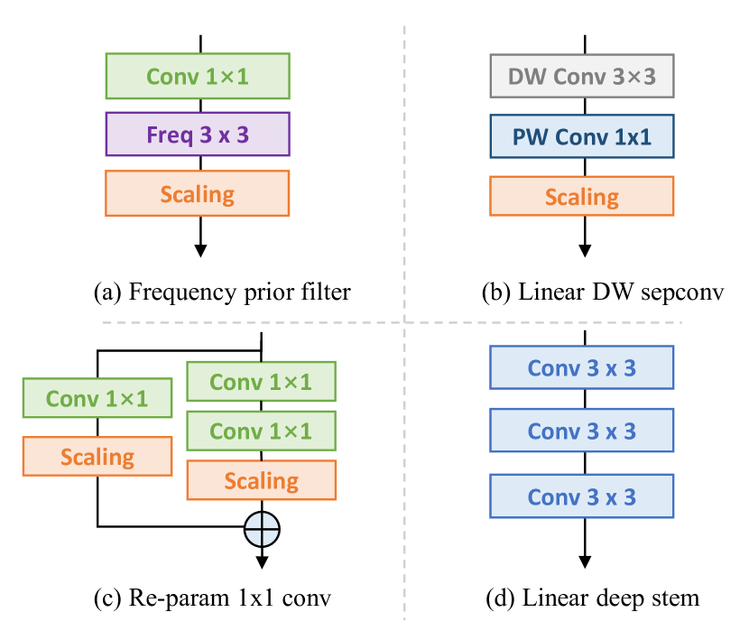
Figure 5: Illustration of the proposed four components in sec:components.

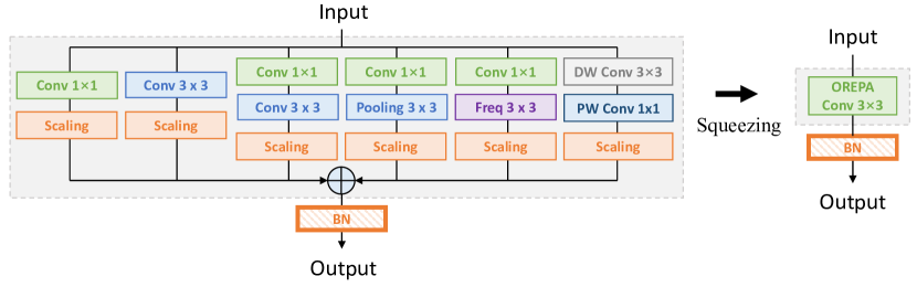
Figure 6: The design of the proposed OREPA block, corresponding to a 3$\times$3 convolution during training and inference.

For each block in the OREPA-ResNet (fig:blocks), i) we add a frequency prior filter and a linear depthwise seperable convolution. ii) We replace all the stem layers (, the initial 7$\times$7 convolution) with the proposed linear deep stem. iii) In the bottleneck [21] blocks, in addition to i) and ii), we further replace the original 1$\times$1 convolution branch with the proposed Rep-1$\times$1 block.

4 Experimental Results

4.1 Implementation Details

We conduct experiments on the ImageNet-1k [13] dataset. We follow the standard data pre-processing pipeline, including random cropping, resizing (to 224$\times$224), random horizontal flipping, and normalization. By default, we apply an SGD optimizer to train the models, with initial learning rate 0.1 and cosine annealed in 120 epochs. We also linearly warm up the learning rate [22] in the initial 5 epochs. We use a global batch size 256 on 4 Nvidia Tesla V100 (32G) GPUs. Unless specified, we use ResNet-18 as the base structure. For a fair comparison, we report results of different models trained under the same settings as described above. For more details, please refer to our supplementary materials.

4.2 Ablation Study

Table 2: Effectiveness of different components in OREPA. We use Top-1 Accuracy to measure the performance. Note that Rep-1$\times$1 is design for the bottleneck blocks, thus not used in ResNet-18.

Model	ResNet-18	ResNet-50
Baseline [21]	71.21	76.70
+ Offline DBB blocks [16]	71.77	76.89
+ Online	71.75	76.86
+ Frequency prior filter	71.78	76.92
+ Linear depthwise separable	71.82	76.98
+ Linear deep stem	72.13	77.09
+ Rep-1$\times$1	-	77.31

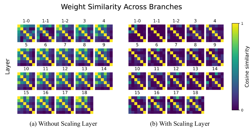
Figure 7: Visualization of branch-level similarity. We calculate cosine similarities between the weights from different branches.

Linear scaling layer and optimization diversity.

We first conduct experiments to validate our core idea, that the proposed linear scaling layers play a similar role as the normalization layers. According to the analysis in sec:principle, we show both the scaling layers and the norm layers are able to diversify the optimization direction. To verify this, we visualize the branch-wise similarity of all the branches in fig:viz. We find that the use of scaling layer can significantly increase the diversity of different branches.

We validate the effectiveness of such diversity in tab:components. Take the ResNet-18 structure as an example, the two kinds of layers (norm and linear scaling) bring similar performance gain (, 0.42 0.40). This strongly supports our claim that it is the scaling part, rather than the statistical-normalization part, that counts most in re-parameterization.

Various linearization strategies.

Table 3: Comparison with linearization variants on the ResNet-18 model. Note that “NaN” means the gradient explosion and the model fails to converge.

Linearization Variants	Top1-Accuracy(%)
Vector scaling	72.13
Scalar scaling	72.04
W/o scaling	71.87
W/o post-addition norm	NaN

We attempt various linearization strategies for the scaling layer. Specifically, we visit four variants.

• Vector: utilize a channel-wise vector and perform the scaling operation along the channel axis.

• Scalar: scale the whole feature map with a scalar.

• W/o scaling: remove the branch-wise scaling layers.

• W/o post-addition norm: remove the post-addition norm layer.

From Table 3 we find that deploying either scalar scaling layers or no scaling layers leads to inferior results. Thus, we choose the vector scaling as the default strategy.

We also study the effectiveness of the post-addition norm layers. As stated in sec:linearization, we add such layers to stabilize the training process. To demonstrate this, we remove such layers, as shown in the last row in tab:linearization, the gradients become infinity and the model fails to converge.

Each component matters.

Next, we demonstrate the effectiveness of the proposed components sec:components. We conduct experiments on both the structures of both ResNet-18 and ResNet-50. As shown in Table 2, each of the components helps to improve the performance.

Online offline.

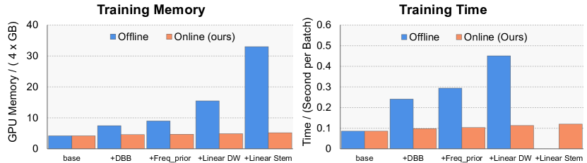
Figure 8: Comparison of training cost between offline re-param method and OREPA.

We compare the training cost of OREPA-ResNet-18 with its offline counterpart (, DBB-18). We illustrate both the consumed memory (fig:budgets(a)) and the training time (fig:budgets(b)). With the increased number of components, the offline re-parameterized model suffers from rapidly increasing memory utilization and the long training time. We can not even introduce deep stem to a ResNet-18 model due to the high memory cost. In contrast, the online re-param strategy accelerates the training speed by 4$\times$, and saves up to 96$+\%$ extra GPU memory. The overall training overhead roughly lies in the same level as that of the base model (vanilla ResNet).

4.3 Comparison with other Re-Param methods

Table 4: Comparison with other re-parameterization models. Note that instead of directly quote results from the original papers, we report models trained on our machine for a fairer comparison.

Model	Re-param	Top1-	GPU-	Training
		Acc	Mem	time/batch
ResNet-18	None	71.21	4.2G	0.086s
	DBB	71.77	7.5G	0.241s
	OREPA	72.13	5.2G	0.120s
ResNet-34	None	74.13	5.2G	0.116s
	DBB	74.83	11.1G	0.424s
	OREPA	75.04	6.7G	0.182s
ResNet-50	None	76.70	10.3G	0.204s
	DBB	76.89	13.7G	0.380s
	OREPA	77.31	11.2G	0.252s
ResNet-101	None	77.71	14.5G	0.382s
	DBB	78.02	19.7G	0.641s
	OREPA	78.29	16.1G	0.445s
RepVGG-A0	RepVGG	72.41	3.8G	0.100s
	OREPA	73.04	4.2G	0.136s
RepVGG-A1	RepVGG	74.46	4.8G	0.121s
	OREPA	74.85	5.5G	0.147s
RepVGG-A2	RepVGG	76.48	5.8G	0.170s
	OREPA	76.72	7.4G	0.210s

We compare our methods with previous structural re-parameterization methods on ImageNet. For the ResNet structure, we compare OREPA-ResNet series with DBB [16]. For a fairer comparison, we report results of DBB trained using our setting. This makes the performances slightly higher than those reported in [16].

From tab:res, we observe that on the ResNet-series, OREPA can consistently improve performances on various models by up to +0.36$\%$. At the same time, it accelerates the training speed by 1.5$\times$ to 2.3$\times$ and saves around 70+$\%$ extra training-time memory caused by re-param. We also conduct experiments on the VGG structure, we compare OREPA-VGG with RepVGG [17]. For the OREPA-VGG models, we simply replace the Conv-3$\times$3 branch with the one we used in OREPA-ResNet. Such a modification only introduces marginal extra training cost, while brings clear performance gain (+0.25%$\sim$+0.6%).

4.4 Object Detection and Semantic Segmentation

To validate the generalization of online re-parameterized models, we apply the pretrained OREPA-ResNet-50 to conduct experiments on the object detection and semantic segmentation tasks. On MS-COCO [29], we train the commonly-used detectors, , Faster RCNN [33] and RetinaNet [28] with default settings in mmdetection [6] for 12 epochs. On Cityscapes, we train the PSPNets [44] and DeepLabV3+ [8] models using mmsegmentation [11] for 40K steps. As show in Table 5, OREPA consistently improves performances on the two tasks.

Table 5: Performance on COCO and Cityscapes validation set with pretrained ResNet-50 backbones. “Mem” is the GPU memory (GB) cost during training and “Time” denotes the average training time of a step (minutes per 50 steps).

Re-param	Faster-RCNN			RetinaNet
	mAP	Mem	Time	mAP	Mem	Time
None	36.5	5.0	0.37	36.2	5.0	0.29
DBB	36.5	6.5	0.46	36.6	6.5	0.40
OREPA	37.0	5.7	0.39	36.9	5.9	0.36
Re-param	PSPNet			DeepLabV3+
	mIoU	Mem	Time	mIoU	Mem	Time
None	74.47	11.5	0.31	76.63	13.1	0.50
DBB	74.50	13.0	0.54	77.15	14.6	0.71
OREPA	75.47	12.3	0.41	77.59	13.8	0.56

4.5 Limitations

When simply transferring the proposed OREPA from ResNet to RepVGG, we find inconsistent performances between the residual-based and residual-free (VGG-like) structures. Therefore, we reserve all the three branches in the RepVGG block to maintain a competitive accuracy, which brings marginally increased computational cost. This is an interesting phenomenon, and we will briefly discuss this in the supplementary materials.

5 Conclusion

In this paper, we present online convolutional re-parameterization (OREPA), a two-stage pipeline aiming to reduce the huge training overhead by squeezing the complex training-time block into a single convolution. To achieve this goal, we replace the training-time non-linear norm layers with linear scaling layers, which maintains optimization diversity and the enhancement of the representational capacity. As a result, we significantly reduce the training-budgets for re-parameterization models. This is essential for training large-scale neural network with complex topologies, and it further allows us to re-parameterize models in a more economic and effective way. Results on various tasks demonstrate the effectiveness of OREPA in terms of both accuracy and efficiency.

Acknowledgments.

This work was supported by the National Key R&D Program of China under Grant 2020AAA0103901, as well as Key R&D Development Plan of Zhejiang Province under Grant 2021C01196. We thank Dongxu Wei and Hualiang Wang for valuable suggestions.

References

- [1] Sanjeev Arora, Nadav Cohen, and Elad Hazan. On the optimization of deep networks: implicit acceleration by overparameterization. In ICML, 2018.
- [2] Jimmy Lei Ba, Jamie Ryan Kiros, and Geoffrey E. Hinton. Group normalization. Stat, 2016.
- [3] Andrew Brock, Soham De, and Samuel L. Smith. Characterizing signal propagation to close the performance gap in unnormalized resnets. In ICLR, 2021.
- [4] Andrew Brock, Soham De, Samuel L. Smith, and Karen Simonyan. High performance large-scale image recognition without normalization. arXiv 2102.06171, 2021.
- [5] Jinming Cao, Yangyan Li, Mingchao Sun, Ying Chen, Dani Lischinski, Daniel Cohen-Or, Baoquan Chen, and Changhe Tu. Do-conv: Depthwise over-parameterized convolutional layer. arXiv 2006.12030, 2020.
- [6] Kai Chen, Jiaqi Wang, Jiangmiao Pang, Yuhang Cao, Yu Xiong, Xiaoxiao Li, Shuyang Sun, Wansen Feng, Ziwei Liu, Jiarui Xu, Zheng Zhang, Dazhi Cheng, Chenchen Zhu, Tianheng Cheng, Qijie Zhao, Buyu Li, Xin Lu, Rui Zhu, Yue Wu, Jifeng Dai, Jingdong Wang, Jianping Shi, Wanli Ouyang, Chen Change Loy, and Dahua Lin. Mmdetection: Open mmlab detection toolbox and benchmark. arXiv preprint arXiv:1906.07155, 2019.
- [7] Ling-Chieh Chen, George Papandreou, Iasonas, Kokkino, Kevin Mupphy, and Alan L. Yuille. Deeplab: semantic image segmentation with deep convolutional nets, atrous convolution, and fully connected crfs. IEEE TPAMI, 2017.
- [8] Liang-Chieh Chen, Yukun Zhu, George Papandreou, Florian Schroff, and Hartwig Adam. Encoder-decoder with atrous seperable convolution for semantic image segmentation. In ECCV, 2018.
- [9] Shoufa Chen, Yunpeng Chen, Shuicheng Yan, and Jiashi Feng. Efficient differentiable neural archetcture search with meta kernels. arXiv 1912.04749, 2019.
- [10] Francois Chollet. Xception: Deep learning with depthwise separable convolutions. In CVPR, 2017.
- [11] Mmsegmentation contributors. Mmsegmentation: Openmmlab semantic segmentation toolbox and benchmark. https://github.com/open-mmlab/mmsegmentation, 2020.
- [12] Soham De and Sam Smith. Batch normalization biases residual blocks towards the identity function in deep networks. In NeurIPS, 2020.
- [13] Jia Deng, Wei Dong, Richard Socher, Li-Jia Li, Kai Li, and Fei-Fei Li. Imagenet: A large-scale hierarchical image database. In CVPR, 2009.
- [14] Xiaohan Ding, Yunchen Guo, Guiguo Ding, and Jungong Han. Acnet: Strengthening the kernel skeletons for powerful cnn via asymmetric convolutional blocks. In ICCV, 2019.
- [15] Xiaohan Ding, Tianxiang Hao, Jianchao Tan, Ji Liu, Jungong Han, Yuchen Guo, and Guiguang Ding. Lossless cnn channel prunning via decoupling remembering and forgetting. In ICCV, 2021.
- [16] Xiaohan Ding, Xiangyu Zhang, Jungong Han, and Guiguang Ding. Diverse branch block, building a convolution as an inception-like unit. In CVPR, 2021.
- [17] Xiaohan Ding, Xiangyu Zhang, Ningning Ma, Jungong Han, Guiguang Ding, and Jian Sun. Repvgg: Making vgg-style convnets great again. In CVPR, 2021.
- [18] Alexey Dosovitskiy, Lucas Beyer, Alexander Kolesnikov, Dirk Weissenborn, Xiaohua Zhai, Thomas Unterthiner, Mostafa Dehghani, Matthias Minderer, Georg Heigold, Sylvain Gelly, Jakob Uszkoreit, and Neil Houlsby. An image is worth 16x16 words: transformers for image recognition at scale. In ICLR, 2021.
- [19] Shuxuan Guo, Jose M. Alvarze, and Mathieu Salzmann. Expandnets: linear over re-parameterization to train compact convolutional networks. In NeurIPS, 2020.
- [20] Kaiming He, Xiangyu Zhang, Shaoqing Ren, and Jian Sun. Delving deep into rectifiers: Surpassing human-level performance on imagenet classification. In ICCV, 2015.
- [21] Kaiming He, Xiangyu Zhang, Shaoqing Ren, and Jian Sun. Deep residual leaning for image recognition. In CVPR, 2016.
- [22] Tong He, Zhi Zhang, Hang Zhang, Zhongyue Zhang, Junyuan Xie, and Mu Li. Bag of tricks for image classification with convolutional neural networks. In CVPR, 2019.
- [23] Andrew G. Howard, Menglong Zhu, Bo Chen, Dmitry Kalenichenko, Weijun Wang, Tobias Weyand, Marco Andreetto, and Hartwig Adam. Mobilenets: Efficient convolutional neural networks for mobile vision applications. arXiv 1704.04861, 2017.
- [24] Jie Hu, Li Shen, and Gang Sun. Squeeze-and-excitation networks. In CVPR, 2018.
- [25] Gao Huang, Zhuang Liu, Laurens van der Maaten, and Kilian Q. Weinberger. Densely connected convolutional networks. In CVPR, 2017.
- [26] Sergey Ioffe and Christian Szegedy. Batch normalization: Accelerating deep network training by reducing internal cobariate shift. In ICML, 2015.
- [27] Alex Krizhevsky, Ilya Sutskever, and Geoffrey E. Hinton. Imagenet classification with deep convolutional neural networks. In NIPS, 2012.
- [28] Tsung-Yi Lin, Priya Goyal, Ross Girshicl, Kaiming He, and Piotr Dollar. Focal loss for dense object detection. In ICCV, 2017.
- [29] Tsung-Yi Lin, Michael Maire, Serge Belongie, Lubomir Bourdev, Ross Girshick, James Hays, Pietro Perona, Deva Ramanan, C. Lawrence Zitnick, and Piotr Dollar. Microsoft coco: Common objects in context. In ECCV, 2014.
- [30] Franck Mamalet and Christophe Garcia. Simplifying convnets for fast learning. In International Conference on Artificial Neural Networks, 2012.
- [31] Zequn Qin, Pengyi Zhang, Fei Wu, and Xi Li. Fcanet: Frequency channel attention networks. In ICCV, 2021.
- [32] Joseph Redmon, Santosh Divvala, Ross Girshick, and Ali Farhadi. You only look once: Unified, real-time object detection. In CVPR, 2016.
- [33] Shaoqing Ren, Kaiming He, Ross Girshick, and Jian Sun. Faster r-cnn: Towards real-time object detection with region proposal networks. In NIPS, 2015.
- [34] Eduardo Romera, Jose M. Alvarez, Luis M. Bergasa, and Roberto Arroyo. Erfnet: Efficient residue factorized convnet for real-time semantic segmentation. IEEE Transactions on Intelligent Transportation System, 2017.
- [35] Tim Salimans and Diederik P. Kingma. Weight normalization: a simple reparameterization to accelerate training of deep neural networks. In NIPS, 2016.
- [36] Shibani Santurkar, Dimit Tsipras, Andrew Ilyas, and Aleksander Madry. How does batch normalization help optimization? In NeurIPS, 2018.
- [37] Jie Shao, Kai Hu, Changhu Wang, Xiangyang Xue, and Bhiksha Raj. Is normalization indispensable for training deep neural networks. In NeurIPS, 2020.
- [38] Karen Simoyan and Andrew Zisserman. Very deep convolutional networks for large-scale image recognition. In ICLR, 2015.
- [39] Min Wang, Baoyuan Liu, and Hassan Foroosh. Factorized convolutional neural networks. In ICCVW, 2017.
- [40] Yuxin Wu and Kaiming He. Group normalization. In ECCV, 2018.
- [41] Sergey Zagoruyko and Nikos Komodakis. Wide residue networks. In BMVC, 2017.
- [42] Hongyi Zhang, Yann N. Dauphin, and Tengyu Ma. Fixup initialization: residual learning without normalization. In ICLR, 2019.
- [43] Mingyang Zhang, Xinyi Yu, Jingtao Rong, and Linlin Ou. Repnas: Searching for efficient re-parameterizing blocks. arXiv 2109.03508, 2021.
- [44] Hengshuang Zhao, Jianping Shi, Xiaojuan Qi, Xiaogang Wang, and Jiaya Jia. Pyramid scene parsing network. In CVPR, 2017.