Supervised Robustness-preserving Data-free Neural Network Pruning

Abstract

When deploying pre-trained neural network models in real-world applications, model consumers often encounter resource-constraint platforms such as mobile and smart devices. They typically use the pruning technique to reduce the size and complexity of the model, generating a lighter one with less resource consumption. Nonetheless, most existing pruning methods are proposed with a premise that the model after being pruned has a chance to be fine-tuned or even retrained based on the original training data. This may be unrealistic in practice, as the data controllers are often reluctant to provide their model consumers with the original data. In this work, we study the neural network pruning in the data-free context, aiming to yield lightweight models that are not only accurate in prediction but also robust against undesired inputs in open-world deployments. Considering the absence of the fine-tuning and retraining that can fix the mis-pruned units, we replace the traditional aggressive one-shot strategy with a conservative one that treats the pruning as a progressive process. We propose a pruning method based on stochastic optimization that uses robustness-related metrics to guide the pruning process. Our method is evaluated with a series of experiments on diverse neural network models. The experimental results show that it significantly outperforms existing one-shot data-free pruning approaches in terms of robustness preservation and accuracy.

1 Introduction

Deep learning is usually realized by a neural network model that is trained with a large amount of data. Compared with other machine learning models such as linear models or support vector machine (SVM) models, neural networks, or more specifically deep neural networks, are empirically proven to gain an advantage in handling more complicated tasks due to their superior capability to precisely approximate an arbitrary non-linear computation [1, 2].

In order to achieve a favorable accuracy and generalization, the common practice to train a neural network is to initialize a model that is large and deep in size. This causes the contemporary models over-parameterized. For example, many models in image classification or natural language processing contain millions or even billions of trainable parameters [3, 4, 5, 6, 7]. Deploying them on resource-constraint platforms, such as the Internet of Things (IoT) or mobile devices, thus become challenging. To resolve this issue, the neural network pruning technique [8, 9, 10] is extensively used. It aims to remove parameters that are redundant or useless, so as to reduce the model size as well as the demand for computational resources.

Most existing research on model pruning assumes the pruning is performed by the model owner who has the original training dataset. The majority of existing pruning techniques are discussed with a premise that the models after being pruned are going to be fine-tuned or even retrained using the original dataset [11, 12, 13, 14, 15]. As a result, they tend to use aggressive and coarse-grained one-shot pruning strategy with the belief that the mis-pruned neurons, if any, could be fixed by fine-tuning and retraining.

This strategy, however, seriously compromises the applicability of pruning. In practice, the model pruning is mostly performed by the model consumers to adapt the model for the actual deployment environment. We refer to this stage as the deployment stage, to differentiate it from the training and tuning stages occurring at the data controller side [16, 17]. In the deployment stage, the model consumers typically have no access to the original training data that are mostly private and proprietary [18, 19]. In addition, data controllers even have to refrain from providing their data due to strict data protection regulations like the EU General Data Protection Regulation (GDPR) [20]. Therefore, pruning without its original training data, which we refer to as data-free pruning, is desirable.

In this work, we approach this problem through the lens of software engineering methodologies. To address the challenge of the lack of post-pruning fine-tuning, we design our pruning as a supervised iterative and progressive process, rather than in a one-shot manner. In each iteration, it cuts off a small set of units and evaluates the effect, so that the mis-pruning of units that are crucial for the network’s decision making can be minimized. We propose a two-stage approach to identify the units to be cut off. At the first stage, it performs a candidates prioritizing based on the relative significance of the units. At the second stage, it carries out a stochastic sampling with the simulated annealing algorithm [21], guided by metrics quantifying the desired property. This allows our method to prune the units that have a relatively low impact on the property, and eventually approaches the optimum.

Our pruning method is designed to pursue robustness preservation, given that the model may be exposed to unexpected or even adversarial inputs [22, 23, 24, 25, 26] after being deployed in a real-world application scenario.

Our solution is to encode the robustness as metrics and embed them into the stochastic sampling to guide the pruning process. It stems from the insight that a small and uniformly distributed pruning impact on each output unit is favored to preserve the robustness of the pruned model. We use two metrics to quantify the pruning impact on the model robustness, namely $L_{1}$-norm and entropy. The $L_{1}$-norm measures the overall scale of pruning impact on the model’s output, in a way that a smaller value tends to incur less uncertainty in the network’s decision making. The entropy measures the similarity of the pruning impact on each output unit. A smaller entropy is obtained in the scenario that the pruning impact is more uniformly distributed in each output unit, and therefore implies that the pruned model is less sensitive when dealing with undesired perturbations in inputs.

We implement our supervised data-free pruning method in a Python package and we evaluate it with a series of experiments on diverse neural network models. The experimental results show that our supervised pruning method offers promising robustness preservation even after 60% of hidden units have been pruned, and meanwhile incurs no significant trade-off in accuracy. It significantly outperforms existing one-shot data-free approaches in terms of both robustness preservation and accuracy, with improvements up to 50% and 30%, respectively. The evaluation also demonstrates that it can generalize on a wide range of neural network architectures, including the fully connected (FC) multilayered perceptron (MLP) models and convolutional neural network (CNN) models.

Contributions

In summary, the contributions of this work are as follows.

• A robustness-preserving data-free pruning framework. We investigate the robustness-preserving neural network pruning in the data-free context. To the best of our knowledge, this is the first work of this kind.

• A stochastic pruning method. We reduce the pruning problem into a stochastic process, to replace the coarse-grained one-shot pruning strategy. The stochastic pruning is solved with the simulated annealing algorithm. This avoids mis-cutting off those hidden units that play crucial roles in the neural network’s decision making.

• Implementation and evaluation. We implement our punning method in Python and evaluate it with a series of experiments on representative datasets and models. To demonstrate the generalization of our method, our evaluation covers not only those models trained on datasets commonly used in the research community such as MNIST and CIFAR-10, but also models designed to solve real-world problems such as credit card fraud detection and pneumonia diagnosis, both of which are robustness-sensitive.

We have made our source code available online (https://github.com/mark-h-meng/nnprune) to facilitate future research on the model pruning area.

2 Background

In this section, we present a brief overview of neural network pruning. We also recap the stochastic optimization and simulated annealing algorithm that are used in our work.

2.1 Neural Network Pruning

A typical deep neural network is a multilayered perceptron architecture that contains multiple fully connected layers [27]. For this reason, deep neural networks are widely recognized as an over-parameterized and computationally intensive machine learning technique [28, 29]. Neural network pruning was introduced in the early 1990s as an effective relief to the performance demand of running them with a limited computational budget [8]. In recent years, as deep neural networks are increasingly applied in dealing with complex tasks such as image recognition and natural language processing, network pruning and quantization are identified as two key model compression techniques and have been widely studied [30, 31, 32, 33, 34, 35, 36, 37, 38, 14, 15]. Existing pruning techniques could be grouped into two genres. One genre of pruning is done by selectively zeroing out weight parameters (also known as synapses). This type often does not really reduce the size and computational scale of a neural network model, but only increases the sparsity (i.e., the density of zero parameters) [39]. Therefore, that genre of pruning is categorized as unstructured pruning in the literature [32, 33]. In contrast, the other genre of pruning called structured pruning emphasizes cutting of entire hidden unit with all its synapses off from which layer it is located, or removal of specific channel or filter from a convolutional layer [13, 40, 31].

Pruning target is the common metric to assess neural network pruning. It indicates the percentage of parameters or hidden units to be removed during the pruning process, and therefore it is also known as sparsity in some literature on unstructured pruning. Fidelity is another metric that describes how well the pruned model mimics the behavior of its original status and is usually calculated through accuracy. An ideal pruning algorithm with promising fidelity should not incur a significant accuracy decline when compared with the original model. However, the discussion of the impact of pruning to measurements beyond fidelity, such as robustness, is still in its nascent phase [41, 42, 43]. As robustness is a representative property specification of a neural network model that concerns the security of its actual deployment, unveiling the influence of pruning on robustness could provide a guarantee to the trustworthiness of pruning techniques.

2.2 Stochastic Optimization

Stochastic optimization refers to solving an optimization problem when randomness is present. In recent years, stochastic optimization has been increasingly used in solving software engineering problems such as testing [44, 45] and debugging [46, 47]. The stochastic process offers an efficient way to find the optimum in a dynamic system when it is too complex for traditional deterministic algorithms. The core of stochastic optimization is the probabilistic decision of its transition function in determining whether and how the system moves to the next state. Due to the presence of randomness, stochastic optimization has an advantage in escaping a local optimum and eventually approaching the global optimum.

The simulated annealing algorithm [21] is an extensively used method for stochastic optimization. It is essentially proposed as a Monte Carlo method that adapts the Metropolis-Hastings algorithm [48] in generating new states of a thermodynamic system. At each step, the simulated annealing calculates an acceptance rate based on the current temperature, generates a random probability, and then makes a decision based on these two variables. In case the generated probability is less than the acceptance rate, the system accepts the currently available neighboring state and accordingly moves to the next state; otherwise, it stays at the current step and then considers the next available neighboring candidate. In general, the simulated annealing algorithm provides an efficient approach to drawing samples from a complex distribution.

3 Problem Definition

In this section, we present the definition of neural network robustness and robustness-preserving pruning.

3.1 Robustness of Neural Networks

Unlike the traditional metrics such as accuracy and loss that mainly focus on the prediction performance during the testing, robustness is a feature representing the trustworthiness of the model against real-world inputs. The real-world inputs may be from an undesired distribution [49], and are often with distortions or perturbations, either intentionally (e.g., adversarial perturbations [23, 50]) or unintentionally (e.g., blur, weather condition, and signal noise [51, 52]). For this reason, robustness is particularly crucial in the open-world deployment of a neural network model.

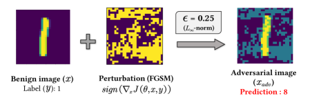
Figure 1: Sample of an adversarial perturbation generated by FGSM, illustrated with a successful attack to the prediction of the MNIST dataset

The evaluation of robustness is discussed against adversarial models, such as projected gradient descent (PGD) attack [24], and fast-gradient sign method (FGSM) [23]. Take FGSM as an example, the adversary can generate an $L_{\infty}$-norm untargeted perturbation for an arbitrary test sample. The untargeted perturbation is calculated with the negative sign of the loss function’s gradient and then multiplied with $\epsilon$ before adding to the benign input. The $\epsilon$ is usually a very small fraction to ensure the adversarial samples are visually indistinguishable from those benign ones [23]. By doing that, an adversarial input tends to maximize the loss function of the victim neural network model and thereby leads the model to misclassify. Fig. 1 illustrates a successful attack that causes the victim model to misclassify an image from the MNIST dataset. The FGSM is regarded as a strong attack model to evaluate the robustness preservation of a neural network model and has been extensively applied in both literature [53, 54, 55] and mainstream toolkits [56, 57]. Accordingly, we adopt FGSM as the default attack model and assume input perturbations are measured in $L_{\infty}$-norm in this work.

Given an adversarial strategy, the attacker can modify an arbitrary benign input with a crafted perturbation to produce an adversarial input. We formalize the robustness property of the neural network model as follows.

Definition 3.1 (Robustness against adversarial perturbations).

Given a neural network model $f$, an arbitrary benign instance $x$ sampled from the input distribution (e.g., a dataset) $X$, and an adversarial input $x_{\text{adv}}$ which is produced by a specific adversarial strategy based on $x$, written as $x_{\text{adv}}=adv\left(x\right)$. The model $f$ satisfies the robustness property with respect to $x$, if it makes consistent predictions on both $x$ and $x_{\text{adv}}$, i.e., $f\left(x\right)=f\left(x_{\text{adv}}\right)$.

3.2 Robustness-preserving Pruning

Our pruning method aims to preserve the robustness of a given neural network model. Following a previous study [22], we define this preservation as the extent that the pruned model can obtain the maximum number of consistent predictions of both benign and adversarial inputs, and accordingly, we name those inputs of consistent predictions as robust instances. Thus, we propose an objective function specifying the number of robust instances from a given distribution. The robustness-preserving pruning then becomes an optimization problem that aims to identify a pruning strategy towards maximizing the objective function. We formalize our goal of robustness-preserving pruning as follows.

Definition 3.2 (Robustness-preserving pruning).

Given a neural network model $f$ that takes inputs and labels from distribution $X$. Each input $x$ has a corresponding label $y$, written as $\left(x,y\right)\in X$. Let $x_{\text{adv}}$ be the adversarial input that adds perturbation to a benign input $x$. Our goal is to find a pruning method $\pi$ that transforms the original neural network model $f$ to a pruned one $g$, which maximizes the objective function $\mathbb{Z}(\pi)$ that counts the occurrence of robust input instances from the distribution $X$, written as:

$$\mathbb{Z}(\pi)=\left|\left\{x|\left(g\left(x_{\text{adv}}\right)=g\left(x\right)=y\right)\land\left(x,y\right)\in X\right\}\right|$$ (1)

4 Approach Overview

In this section, we introduce our primitive pruning operation to show how individual unit is pruned, and then give a brief overview of our approach.

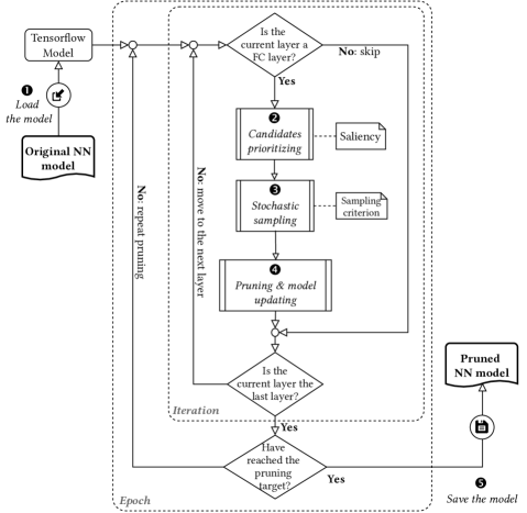
Figure 2: The workflow of our pruning method

4.1 Saliency-based Primitive Pruning Operation

When attempting to prune a hidden unit (denoted by the nominee, i.e., the one chosen to be pruned), our method uses a pair-wise strategy rather than simply deleting the nominee. In particular, our primitive pruning operation considers another unit (denoted by the delegate, i.e., the one to cover the nominee’s duty) from the nominee’s layer that tends to play a similar role in making a prediction. It removes the nominee and adjusts the parameters of the delegate so that the impact of a single pruning operation on the subsequent layers can be reduced. Given a nominee and delegate pair $\left<a^{l}_{i},a^{l}_{j}\right>$, which are the $i$-th and $j$-th hidden units at the layer $l$, the primitive pruning operation performs the following two steps.

1. The nominee $a^{l}_{i}$ is pruned. To this end, we zero out all parameters connecting from and to $a^{l}_{i}$;

2. We modify the parameters connecting from the delegate $a^{l}_{j}$ to the next layer with the sum of the parameters of both $a^{l}_{i}$ and $a^{l}_{j}$.

The parameter update in Step (2) is carried out to offset the impact caused by pruning the nominee. Fig. 3 illustrates our primitive pruning operation.

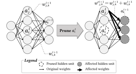
Figure 3: An illustration of the primitive pruning operation on $\left<a^{l}_{i},a^{l}_{j}\right>$

To find the delegate, we use a metric called saliency, which is proposed in a previous study [40] to assess the “importance” of a unit when it is to be replaced by another unit in its layer. A lower saliency means that the nominee can be replaced by the delegate with less impact on the network. Let $w^{l}_{i,j}$ be the weight parameter connecting the $i$-th hidden unit at the layer $l-1$ with the $j$-th hidden unit at the layer $l$, and $b^{l}_{i}$ be the bias parameter of the $i$-th hidden unit at the layer $l$. Given the nominee $a^{l}_{i}$, its saliency with respect to the delegate $a^{l}_{j}$ is measured as follows.

$$S\left(a^{l}_{i},a^{l}_{j}\right)=\frac{\sum{W^{l+1}_{i,*}}}{\left|W^{l+1}_{i,*}\right|}\times\left(\lVert W^{l}_{*,i}-W^{l}_{*,j}\rVert_{2}+\frac{\left|b^{l}_{i}-b^{l}_{j}\right|}{\left|b^{l}_{i}+b^{l}_{j}\right|}\right),\\ \qquad\qquad\qquad\qquad\text{where}\;W_{i,*}^{l}=\left\{w_{i,m}^{l}|a_{m}^{l}\in a^{\left[l\right]}\right\},W_{*,i}^{l}=\left\{w_{n,i}^{l}|a_{n}^{l}\in a^{\left[l-1\right]}\right\}$$ (2)

4.2 Workflow of the Pruning Method

Fig. 2 shows the workflow of our pruning method. It begins with reading a pre-trained model and loading its architecture and parameters (Stage ❶). Then it traverses the model layer by layer and iteratively performs hidden unit pruning. The pruning process (Stage ❷-❹) might be executed in multiple epochs, depending on the pruning target and pruning batch size per epoch. Once the pruning target has been reached, our method saves the pruned model (Stage ❺).

Below we brief each component in the pruning process. The outer loop specifies an epoch, in which a fixed portion of fully connected units (i.e., the batch size) will be cut off from the model. The inner loop represents the iteration of all layers in a forward direction. A pruning iteration is composed by three stages, i.e., candidates prioritizing (Stage ❷), stochastic sampling (Stage ❸) and pruning and model updating (Stage ❹). The former two stages identify the units to be pruned at each iteration, and then our method invokes the primitive pruning operation to prune each of them.

• The candidates prioritizing stage evaluates the saliency for every pair of hidden units at the beginning of each iteration and generates a saliency matrix. Considering that pruning a nominee that is hard to find a proper delegate (i.e., the nominee has high saliency with respect to every hidden unit in its layer) is unfavorable, we sort the list of hidden unit pairs according to their saliency values in ascending order and pass that list to the next stage. Those candidates with the least saliency values are given priority to be processed in the next stage.

• The stochastic sampling stage takes the list of pruning candidates as input and identifies the units to be pruned. The basic idea is to estimate how pruning a unit impacts the prediction at the output layer, to decide whether to keep or discard it. A naive way is to evaluate the impact of each candidate, but this is too costly since calculating each impact requires a forward propagation till the output layer. We thus employ a stochastic sampling strategy with the estimated impact as a guide in this process. Our impact estimation and corresponding sampling strategy are detailed in Section 5.

5 Supervised Data-free Pruning

In this section, we introduce our supervised pruning method. We detail our approach of estimating how pruning a unit impacts the prediction at the output layer (Section 5.1). With this, we can approximate the cumulative impact on the robustness of the final model, and thus we embed it into our sampling criterion (Section 5.2). To prevent the sampling method from being stuck at a local optimum, we employ the simulated annealing algorithm in determining which candidate(s) to prune (Section 5.3).

5.1 Estimation of Pruning Impact

Because the primitive pruning operation prunes the nominee and modifies the value of parameters connecting from the delegate to the next layer, it affects the computation of the hidden units in subsequent layers. Such impact would eventually propagate to the output layer. In this section, we discuss how we estimate this impact.

For an original model $f$ that performs an $n$-class classification, its output, when given a sample $x$, is a vector of $n$ numbers denoted by $f\left(x\right)=\left[o_{1},...,o_{n}\right]$. The model $g$, which is derived by pruning a unit of $f$, outputs another vector of the same size, denoted by $g\left(x\right)=\left[o^{\prime}_{1},...,o^{\prime}_{n}\right]$. We aim to estimate the impact at the output layer as a vector of $n$ items, i.e., $g\left(x\right)-f\left(x\right)$ for any legitimate input. To achieve this, we first approximate the valuation of hidden units involved in the candidate pair (i.e., nominee and delegate) by interval arithmetic based on the bounds of normalized input. Next, we assess the impact caused by a primitive pruning operation on the subsequent layer where the pruning operation is performed. In this process, we quantify the impact as an interval. After obtaining the impact on the subsequent layer, we apply the forward propagation until the output layer, so that the pruning impact on the output layer can be derived.

We adopt the abstract interpretation that is commonly used in the literature of neural network verification [58, 59, 60] to estimate the upper and lower bounds of an arbitrary hidden unit. To achieve that, we need to define the scope of a legitimate input as an interval. As input normalization is a common preprocessing practice prior to training a neural network, the value of an input feature is usually restricted to a fixed range (e.g., $\left[0,1\right]$). With a vector of intervals provided as the input, we perform the forward propagation to approximate the valuation of the involved hidden units. This propagation simulates the computation within a neural network model with a specific input. During the propagation, we leverage the interval arithmetic rules [60] to calculate the upper and lower bounds. In the actual implementation, we build a map of intervals for all hidden units of the neural network at the beginning of pruning. Due to each primitive pruning modifies parameters at the next layer, we update the map with the latest estimation after each iteration specifies the batch pruning at the same layer.

For an arbitrary hidden unit at the $\left(l+1\right)$-th layer $a^{l+1}_{k}\in a^{\left[l+1\right]}$, its impact caused by a primitive pruning of $\left<a^{l}_{i},a^{l}_{j}\right>$ can be formulated as Eq.3 below.

$$\begin{split}\Delta a_{k}^{l+1}&=\left(w^{l+1}_{j,k}+w^{l+1}_{i,k}\right)\times a^{l}_{j}-\left(w^{l+1}_{i,k}\times a^{l}_{i}+w^{l+1}_{j,k}\times a^{l}_{j}\right)\\ &=w^{l+1}_{i,k}\times\left(a^{l}_{j}-a^{l}_{i}\right)\end{split}$$ (3)

We can obtain the latest estimation of both $a^{l}_{i}$ and $a^{l}_{j}$ from the map of intervals that we have built at the beginning. Since all weight parameters are known in the white-box setting, we can also quantify the impact $\Delta a_{k}^{l+1}$ as an interval.

Next, we perform another round of forward propagation to simulate the impact of affected hidden units from the layer $l+1$ to the output layer. The value to be propagated in this round is no longer the interval of input, but the impact of affected hidden units as intervals. The propagated impact at the output layer could be treated as the estimated result of $g\left(x\right)-f\left(x\right)$ for the current pruning operation. The propagated impact on the output for each pruning operation will be accumulated along with the pruning progress. We call it cumulative impact to the output layer and use $\Delta a^{\left[out\right]}$ to denote it in the remaining of this section.

5.2 Sampling Criterion

Our sampling criterion is proposed based on an insight that a small and uniformly distributed cumulative impact is less possible to drive the pruned model to generate an output that is different from the original one, even the input is with an adversarial perturbation. On the contrary, the pruning impact with a variety of scales and values is considered to impair the robustness because it makes the pruned model sensitive that its prediction may flip when encountered a perturbation in the input. Our proposed criterion is composed of two sampling metrics.

• One metric accounts for the scale of cumulative impact on the output layer. A greater scale means the current pruning operation generates a larger magnitude of impact on the output layer.

• The other is based on the entropy that assesses the degree of similarity of cumulative impact on each output unit. A greater entropy implies the pruning impact on each output node shows a lower similarity.

Our sampling strategy jointly considers both metrics and favors both to be small.

Metric #1: Scale

As we can obtain the cumulative impact as a vector of intervals, we adopt the $L_{1}$-norm to assess the scale of cumulative impact. Here we use $\left(u^{-},u^{+}\right)$ to represent the impact bounds of an arbitrary node $u$ at the output layer and let the term $NORM$ denote the $L_{1}$-norm of the intervals. The formula to calculate $NORM$ is shown in Eq. 4.

$$NORM\left(\Delta a^{\left[out\right]}\right)=\sum_{\left(u^{-},u^{+}\right)\in\Delta a^{\left[out\right]}}{\left|u^{+}-u^{-}\right|}$$ (4)

Metric #2: Entropy

We apply Shannon’s information entropy [61] to measure the similarity of cumulative impact on each output unit. Our measurement of the similarity for a pair of intervals is adopted from existing literature [62, 63, 64], as defined below.

Definition 5.1 (Similarity of interval-valued data).

Given a list of intervals $U=\left\{u_{1},u_{2},...,u_{3}\right\}$, and each interval is composed of its lower and upper bounds such as $u_{i}=\left[u_{i}^{-},u_{i}^{+}\right]$. Let $m^{-}=\min_{u_{i}\in U}\left\{u_{i}^{-}\right\}$ be the global minimum of $U$, i.e., the minimum of lower bounds, and similarly, $m^{+}=\max_{u_{i}\in U}\left\{u_{i}^{+}\right\}$ be the global maximum. The similarity degree of relative bound difference between two intervals $u_{i}$ and $u_{j}$ is defined as:

$$Sim_{ij}=1-\frac{1}{2}\frac{\left|u_{i}^{-}-u_{j}^{-}\right|+\left|u_{i}^{+}-u_{j}^{+}\right|}{m^{+}-m^{-}}$$ (5)

With this definition, we say two intervals $u_{i}$ and $u_{j}$ are $\phi$-similar if $Sim_{ij}\geq\phi$ for any similarity threshold $\phi=\left[0,1\right]$.

Next, we measure the overall similarity of an interval with all other intervals in a list, and we call it density of similarity. We adopt the calculation of the density of $\phi$-similarity for an interval from an existing study [64], which is defined as follows.

Definition 5.2 (Density of similarity).

For an interval $u_{i}$ from a list of intervals $U=\left\{u_{1},u_{2},...,u_{3}\right\}$, its density of $\phi$-similarity among $U$ is measured by the probability of an arbitrary interval (other than $u_{i}$) is $\phi$-similar with itself, calculated as:

$$\rho_{\phi}\left(u_{i}\right)=\frac{\left|\left\{u_{j}|Sim_{ij}\geq\phi,\forall u_{j}\in U\backslash\left\{u_{i}\right\}\right\}\right|}{\left|U\right|}$$ (6)

With the density of similarity, we define the metric as the entropy of the cumulative impact on the output layer, written as $ENT$. The formula of $ENT$ calculation is presented in Eq.7.

$$ENT\left(\Delta a^{\left[out\right]}\right)=-\sum_{u_{i}\in\Delta a^{\left[out\right]}}{\rho_{\phi}\left(u_{i}\right)\cdot\log\rho_{\phi}\left(u_{i}\right)}$$ (7)

The similarity threshold $\phi$ is in the range $\left[0,1\right]$. With the same set of intervals, a higher $\phi$ results in a lower density of similarity such that it makes entropy calculation more sensitive to the difference of those intervals. In our work, the cumulative impact is obtained after a forward propagation of several layers and therefore might be in a large magnitude. Accordingly, we set 0.9 as the default value of $\phi$ to maintain a variety of similarity densities rather than all equal to one.

Synthesis

We introduce a pair of parameters $(\alpha,\beta)$ to specify the weight of these two metrics. Considering these two metrics may have different magnitude, and particularly, the $NORM$ is unbounded (i.e., no upper bound), we use a sigmoid function ($\sigma$) to normalize these two metrics in the final criterion. Due to the concave and monotonic nature of sigmoid logistic function for values greater than zero, it can output bounded results within $\left(-1,1\right)$ with their values’ order the same with input, denoted as $x_{1}<x_{2}\Leftrightarrow\sigma\left(x_{1}\right)<\sigma\left(x_{2}\right)$. On the whole, the definition of our sampling criterion is given in Eq. 8 below.

$$\begin{split}Energy_{\left(\alpha,\beta\right)}\left(\Delta a^{\left[out\right]}\right)=\alpha\cdot\sigma\left(NORM\left(\Delta a^{\left[out\right]}\right)\right)+\beta\cdot\sigma\left(ENT\left(\Delta a^{\left[out\right]}\right)\right),\qquad&\\ \text{subject to}\;\alpha\geq 0,\beta\geq 0,\beta=1-\alpha&\end{split}$$ (8)

We use the term energy to represent our sampling criterion to echo the simulated annealing algorithm used in our guided stochastic sampling strategy, which will be presented in the next subsection.

5.3 Guided Stochastic Sampling

Since the sampling criterion can reflect the impact of the unit pruning on the model robustness, a naive way is to calculate $energy$ (Eq. 8) for every pair and prune the unit with the least value. However, this is too expensive because each calculation requires a forward propagation in a fully connected manner. To address this, we use a stochastic sampling guided by the $energy$-based heuristic to identify the candidates to be pruned. Our method is presented in Algorithm 1, and we discuss it in the remainder of this section.

Algorithm 1 Supervised pruning with a stochastic heuristic

0:  An $n$-layer neural network model to be pruned ($q_{t-1}$), cumulative impact of all previous pruning ($\Delta a^{\left[out\right]}$), weights used in sampling criterion ($\alpha,\beta$), batch size ($k$), current temperature $T_{t-1}$

0:  A pruned deep learning model $q_{t}$, updated cumulative impact of pruning $\Delta a^{\left[out\right]}$, the list of hidden units pruned $p^{l}$, the updated temperature $T_{t}$

1:  for layer $l$ in all hidden layers do

2:     load parameters of the current layer $\Sigma_{l}$

3:     build a saliency matrix $M^{l}$ for the unit pairs

4:     sort the saliency matrix $M^{l}$ in ascending order

5:     set $energy_{t-1}\leftarrow 0$

6:     for hidden unit pair $p:\left<i,j\right>$ in the first $k$ values in $M^{l}$ do

7:        simulate a pruning of $p$ and calculate the impact on the output layer $\Delta_{p}$

8:        calculate the temporary cumulative impact $temp\Delta a^{\left[out\right]}\leftarrow\Delta a^{\left[out\right]}+\Delta_{p}$

9:        calculate $NORM$ and $ENT$ with $temp\Delta a^{\left[out\right]}$

10:        calculate the sampling criterion $energy^{\prime}\leftarrow\alpha\cdot\sigma\left(NORM\right)+\beta\cdot\sigma\left(ENT\right)$

11:        if ($energy_{t-1}>0$) and ($energy^{\prime}>energy_{t-1}$) then

12:           calculate acceptance rate $P$ based on temperature $T_{t-1}$ and $energy^{\prime}$

13:           generate a random probability $rand$

14:           if ($rand\geq P$) then

15:              reject the current $p$ and go to the next one

16:           end if

17:        end if

18:        accept and perform pruning $q_{t}\leftarrow\delta\left(q_{t-1},p\right)$

19:        add $p$ into a pruning list $P^{l}$

20:        update $energy_{t-1}\leftarrow energy^{\prime}$

21:     end for

22:     update $\Delta a^{\left[out\right]}$ with pruning $P^{l}$

23:     update temperature $T_{t}\leftarrow T_{t-1}$

24:  end for

We exploit the idea of simulated annealing to implement our sampling strategy through the lens of stochastic optimization. In particular, our method traverses the hidden unit pairs from the candidates prioritizing result one by one. In the beginning, our method by default accepts the first candidate from the prioritizing result and records its $energy$ as the evaluation of the current state. Upon receiving a new pruning candidate, the method calculates the $energy$ of that candidate, compares it with the current state, and decides whether to prune it during the current iteration, according to an acceptance rate calculated based on a temperature variable $T$. The temperature variable is adopted from the thermodynamic model. The descent of temperature value reflects the solving progress of the optimization problem – as temperature decreases, our method would less possibly accept a pruning candidate with an $energy$ greater than the current state. Here we define the temperature used in our method as the portion of the remaining pruning task, which equals 1 at first and approaches 0 when the pruning target is reached. Given the temperature of the current iteration written as $T_{t-1}$, the assessment of the last drawn (accepted) candidate $energy_{t-1}$, we can obtain the acceptance rate of the next candidate (line 12 of Algorithm 1) once we calculate its energy (written as $energy^{\prime}$, line 10) according to Eq. 8. The formula of acceptance rate is provided as follows.

$$P=\min\left(1,\exp\left(-\frac{energy^{\prime}-energy_{t-1}}{T_{t-1}}\right)\right)$$ (9)

As Eq. 9 shows, our method automatically accepts a candidate if its $energy$ is lower than the one in the current state; otherwise, a random probability will be generated and tested against the acceptance rate to determine whether we accept or discard the candidate. This procedure is reflected as lines 11-20 of Algorithm 1.

There are two obvious advantages of this stochastic process. First, applying such randomization in sampling is less expensive than computing $energy$ of all candidates and sorting. Moreover, the stochastic process through simulated annealing enables us to probabilistically accept a candidate that may not have the lowest $energy$ at the current step. This helps prevent our pruning method from being stuck at a local optimum and eventually achieves our objective.

6 Evaluation

This section presents the evaluation of our pruning method. We aim to answer the following three research questions.

• RQ1: Robustness Preservation. How effective is our pruning method in terms of robustness preservation? Does it cause significant decay on the model accuracy? Does our method generalize on diverse neural network models?

• RQ2: Pruning Efficiency. Can our method complete the pruning within an acceptable time?

• RQ3: Benchmarking. Can our method outperform one-shot strategies in terms of robustness preservation?

6.1 Implementation and Experiment Settings

We implement our pruning method into a Python program. All neural network models are trained, pruned, and evaluated based on TensorFlow v2.3.0. Our toolkit accepts any legitimate format of neural network models trained by TensorFlow. It also allows the user to configure the pruning target and the number of pruning per epoch. Given a model as input, it automatically identifies the fully connected hidden layers, prunes the hidden units from those layers, and stops once the pruning has reached the setting threshold (e.g., 80% of hidden units have been cut off). Our source code is made available online to facilitate future research on similar topics.

To evaluate our method on diverse mainstream neural network applications, we select four representative datasets ranging from structured tabular data to images, with labels for both binary classification and multi-class classification. For each dataset, we select a unique architecture of neural network model to fit the classification task. To this end, we refer to the most popular example models on Kaggle. We have trained four models with different architectures, covering both purely fully connected MLPs and CNNs. All models are trained with a 0.001 learning rate and 20 epochs. The number of fully connected layers and hidden units per layer varies among these models. Besides that, we also test our method with models that use different activation functions. We have trained another two models separately with ReLU and sigmoid for each of MNIST and CIFAR-10 datasets respectively. The diversification of the models is to evaluate the generalizability of our method (RQ1). The details of the four used datasets and six pre-trained models are listed in Table 1.

Table 1: Datasets and models used in evaluation

Models			Model Architecture	Activation
No.	Dataset	Type & Input Size
1	Credit Card Fraud Detection [65]	Tabluar data (30 columns)	4 layer MLP ($64\times 64\times 2$)	ReLU
2	Chest X-ray Images (Pneumonia) [66]	Colored images (various sizes)	19 layer CNN (w. 2 FC layers) ($128\times 2$)	ReLU
3	MNIST Handwritten Digits [67]	Greyscale images ($28\times 28$)	5 layer MLP ($128\times 128\times 64\times 10$)	ReLU
4	MNIST Handwritten Digits [67]	Greyscale images ($28\times 28$)	5 layer MLP ($128\times 128\times 64\times 10$)	sigmoid
5	CIFAR-10 Images [68]	Colored images ($32\times 32$)	9 layer CNN (w. 3 FC layers) ($128\times 64\times 10$)	ReLU
6	CIFAR-10 Images [68]	Colored images ($32\times 32$)	9 layer CNN (w. 3 FC layers) ($128\times 64\times 10$)	sigmoid

We empirically select the values of the parameters $\alpha$ and $\beta$ through a tuning process. . We observe the pruning of those multi-class models like MNIST and CIFAR-10 is more sensitive to their values compared with binary classification models. We also find that $\alpha=0.75$ suits the models that use ReLU as activation, and $\alpha=0.05$ suits those sigmoid models. The reason for such difference lies in the importance of $L_{1}$-norm of pruning impact on the output layer. As the sigmoid activation function always tends to converge to a fixed interval, different sampling decision does not make much difference in the $L_{1}$-norm of cumulative pruning impact at the output layer. Thus, we give more weight to the entropy when pruning sigmoid models. Our experiments run on an Ubuntu 20.04 LTS machine with an 8-core Intel CPU (2.9GHz Core (TM) i7-10700F), 64GB RAM and an NVIDIA GeForce RTX 3060Ti GPU.

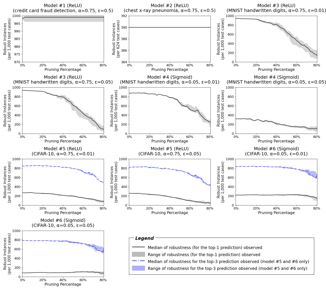
Figure 4: Robustness decay of six models when applying our supervised pruning method (up to 80% pruning)

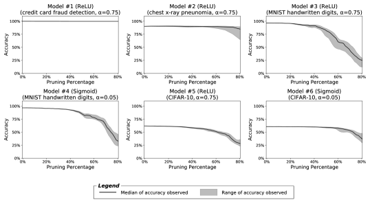
Figure 5: Accuracy decay of six models when applying our supervised pruning method (up to 80% pruning)

6.2 RQ1: Robustness Preservation

Our first set of experiments is conducted to investigate the robustness preservation of our pruning method. We apply the method on all six models. The used metric of robustness preservation is based on Definition 3.2. Our evaluation calculates the number of consistent and correct classification of adversarial inputs on both the original and pruned models, and compares these two numbers to determine the degree of robustness preservation. In addition, we notice that the models trained on CIFAR-10 tend to be more sensitive to adversarial inputs compared with the counterparts trained on simpler datasets like MNIST, as revealed by previous studies [22, 24]. Therefore, for models trained on it, i.e., models #5 and #6, we also evaluate the preservation of the top-$K$ ($K=3$ in our experiment) prediction results, which is another metric that has been commonly adopted in machine learning evaluation [4, 69, 70].

As previous studies have shown that pruning may cause decay of classification accuracy [40, 32], we also test the accuracy of the pruned models to explore the impact of our method on it. This is crucial because a poor accuracy would undermine the validity of robustness which only requires the model not to produce inconsistent outputs for a given benign input and its adversarial variant, regardless of whether the benign input is correctly predicted or not. With the overall pruning target set as 80% of hidden units being pruned, our method prunes the same proportion of units per layer at each iteration. After each pruning epoch, we evaluate the robustness and accuracy of the models.

Fig. 4 shows the robustness preservation of our method on all six models listed in Table 1, against untargeted FGSM adversaries with different epsilon ($\epsilon$) options. This parameter is used in FGSM to measure the variation between the adversarial and benign samples. We refer to the literature [22, 23, 56] to find proper values to use in our experiment. We perform 15 rounds of experiments on all six models and plot the range (the shaded area) and the median (the curve) of the experimental results in the figure. We also track the change of accuracy for each model during the pruning process and present the results in Fig. 5. In general, our method performs well on all six models. The pruning imposes almost no impact on the robustness and accuracy of models #1 and #2, even when 80% of units are cut off. On the models for binary classification, i.e., models #1 and #2, our method imposes almost no impact on the robustness and accuracy, even when 80% of units are pruned. For those models with more complex classification tasks, i.e., models #2-#6, our method still achieves favorable results. All four models preserve at least 50% of their original robustness even after 60% of hidden units are pruned. The change of the classification accuracy generally shares the same trend as robustness (see Fig. 5). All models still preserve 50% of their original accuracy when 70% of their units have been pruned.

In some cases, e.g., model #6 with sigmoid, we observe that the robustness slightly grows as the number of pruned units increases. This is because these models are not trained with robustness preservation as part of the objective functions, and our pruning guided by that metrics which incorporate robustness preservation may enhance their robustness. This on the other hand demonstrates the effectiveness of the robustness preservation of our method.

Our first set of experiments has responded to RQ1. In summary, our pruning method shows favorable robustness preservation against adversarial perturbations. Although our method is not designated to preserve the model accuracy, it does not show any drastic performance decay along with the pruning progress. Our method is also able to generalize on many types of models, as shown by the evaluation outcomes of all six representative models.

Table 2: Time consumed in pruning 80% of fully connected parameters (average of 10 executions)

Model	Number of parameters	Batch size per layer	Elapsed time ($10^{2}$ seconds)
#1 (Credit card fraud)	6,145	3.13%	0.350
#2 (Chest x-ray)	131,329	1.56%	1.840
#3 (MNIST, ReLU)	125,898	1.56%	4.354
#4 (MNIST, sigmoid)	125,898	1.56%	4.371
#5 (CIFAR-10, ReLU)	140,106	1.56%	2.653
#6 (CIFAR-10, sigmoid)	140,106	1.56%	2.693

6.3 RQ2: Pruning Efficiency

To explore the efficiency performance of our method, we run it on the six models with a “worst-case setting”. Specifically, we examine the case of pruning a large proportion (80%) of the entire model, in the slowest pace (1 or 2 per layer per epoch). This gives our method disadvantages, but when applied in practice, it could be much more efficient.

Table 2 details the time consumed by our method on each of the six models. In general, our method can prune a model within an acceptable time. In the multi-class prediction models, the pruning process can be completed within 8 minutes, while in the binary classification models, the process can be completed much faster.

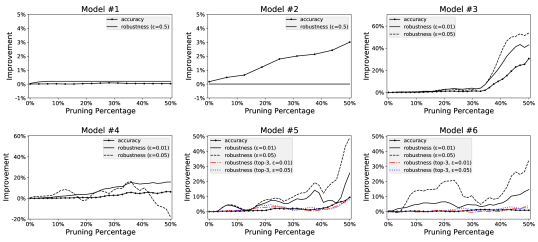
Figure 6: Improvement of our method against saliency-based one-shot pruning on six models

6.4 RQ3: Benchmarking

Our second set of experiments is conducted to explore whether our method can outperform existing one-shot data-free pruning methods. We compare its performance with that of the saliency-based one-shot pruning, which is a commonly used approach to perform data-free neural network pruning [40, 32]. We note that our evaluation focuses on the comparison of data-free pruning techniques, and we refer the reader to the existing study [33] that compares performance between data-driven and data-free pruning techniques.

We reuse the same six models and take the saliency-based one-shot pruning as the baseline. The improvement of robustness is calculated as the growth in the number of robust instances observed from running our method relative to the counterpart observed from running the baseline method. The improvement of accuracy is equal to the growth of accuracy of the pruned model produced by our method relative to the one pruned by the baseline method.

The experimental results show our method outperforms the saliency-based one-shot pruning in overall settings. In the experiments on MNIST and CIFAR-10 models (i.e., models #3-#6) with ReLU activation, as shown in Fig. 6, our method achieves a significant improvement in both robustness preservation (up to 50%) and accuracy (up to 30%). Compared with the binary classification models (i.e., models #1 and #2), our method achieves more significant improvement on those with complicated structures and are sensitive to adversarial inputs. Five out of the six models can be pruned with a higher accuracy and robustness preservation compared with the baseline. There is an exception found in model #4 that our method fails to outperform the baseline after 40% units have been pruned, but it still well preserves the robustness during the pruning process as shown in Fig. 4 (the subplot at row 2 and column 3).

Table 3: Demonstration of robustness original and pruned models (misclassification results are shown in bold and italic font)

To demonstrate our improvement, we randomly select two samples from both MNIST and CIFAR-10 datasets, apply FGSM attack on them, and test them on our method and the baseline method. The classification outcome of those adversarial inputs compared with the original labels are depicted in Table 3. The models after our pruning have shown better robustness against adversarial perturbations than those pruned by the baseline method. We observe that all four instances are correctly classified after 25% pruning, and three out of four instances are correctly classified even after 50% pruning.

We also observe the change in robustness preservation of a model is dependent on the utilization of its hidden units. In particular, the improvement of our pruning starts declining after 38% and 25% units are pruned in the two models of CIFAR-10, but this phenomenon does not appear in the remaining models. Models #1-#4 are trained as fully connected MLPs, while the models of CIFAR-10 are trained as CNNs with only a small portion of their units are fully connected. This makes the former models contain more computationally negligible parameters than the models of CIFAR-10, and therefore the pruning of the former yields less impact on the robustness than the latter ones.

7 Threats to Validity

Our work focuses on robustness-preserving data-free pruning, which has not been well studied by our research community, compared with the pruning with a retraining option. To the best of our knowledge, this is the first one that uses the stochastic approach to address the pruning problem. However, it carries several limitations that should be addressed in future work.

First, our method is primarily designed for fully connected components of a neural network model. Fully connected layers are fundamental components of deep learning and have been increasingly used in state-of-the-art designs such as MLP-Mixer [6]. Nevertheless, our method may be limited when applied to models with convolutional and relevant layers (e.g., pooling and normalization) playing a major role. We still need to explore more regarding how to effectively prune diverse models that are not built in conventional fully connected architecture, such as transformer models.

Second, our pruning heavily relies on interval arithmetic in approximating the valuation of hidden units and pruning impact, so the precision of those intervals determines both the effectiveness and correctness of our method. When it is applied to a ReLU-only model with a fully connected multilayered perceptron, there may be a magnitude explosion issue during our evaluation of propagated impact on the output layer. Besides, pruning a model mixed with both convergent (e.g., sigmoid) and non-convergent (e.g., ReLU) activation may be challenging for our method, because a convergent activation may reduce the quantitative difference from the previous assessment and output a similar result close to $\left(-1,1\right)$ — this may reduce the effectiveness of our sampling criterion.

We share our insight for future work to mitigate these limitations in two aspects. First, the data-free pruning could be extended to more layer types especially those over-parameterized layer types like 2D convolutional layer. Additional pruning criteria may address the first limitation. Second, a more precise interval approximation or refinement technique could be applied to optimize the pruning criteria. By doing this the magnitude explosion issue of the propagated impact on the output layer may be relieved.

8 Related Work

Unstructured Pruning & Structured Pruning

Existing pruning approaches can be classified into two classes, namely unstructured pruning, and structured pruning [32]. Unstructured pruning is also known as individual weight pruning, which is performed to cut one specific (redundant) parameter off the target neural network model at a time. Unstructured pruning could date back to the early era when network pruning was first introduced and covers many well-known representative studies such as Optimal Brain Damage [8] and Optimal Brain Surgeon [71]. They typically prune weight parameters based on a Hessian of the loss function. Other studies that can be categorized as unstructured pruning include [33, 72].

Structured pruning is proposed to prune a neural network model at the hidden unit, channel, or even layer level. Hu et al. [37] proposed a channel pruning technique according to the average percentage of zero outputs of each channel, while another study by Li et al. [38] presented a similar channel pruning but according to the filter weight norm. Besides that, pruning a channel or layer with the smallest magnitude, there is another common approach discussed in [35, 12] that prunes a hidden unit, channel, or layer with the least influence to the final loss. He et al. [34] and Luo et al. [13] proposed channel pruning based on consequential feature reconstruction error at the next layer. Srinivas and Babu [40] introduced a data-free parameter pruning methodology based on saliency, which performs hidden unit pruning independently of the training process and as the result, does not need to access training data. The latest work also includes [14] that considers the inter-correlation between channels in the same layer. Another work by Chin et al. [36] proposes a layer-by-layer compensate filter pruning algorithm.

In-training Pruning & Post-training Pruning

On the other hand, depending on when the parameters’ pruning is performed, we can also categorize existing pruning strategies as either in-training pruning or post-training pruning (also known as data-free pruning) [73]. Besides a few papers that discuss post-training pruning [74, 40], most existing studies such as [37, 75, 8, 71, 76] are implemented as in-training pruning.

One representative in-training pruning approach named SNIP [76] achieves single-shot pruning based on connection sensitivity and has been exhaustively compared with existing techniques. Hornik et al. [1] investigated a data-agnostic in-training pruning that proposes a saliency-guided iterative approach to address the layer-collapse issue. In-training pruning gives us a chance to fine-tune or even retrain the pruned network with the original dataset, and therefore it is capable to prune a larger portion of the neural network without worrying about a severe impact on the performance (e.g., accuracy and loss). A recent empirical study performed by Liebenwein et al. [43] reveals the robustness could be well preserved during the mainstream in-training pruning. Even though, post-training like [40, 74] still has its market to reduce the size of a pre-trained ready-to-use neural network model from a user’s perspective. The effectiveness of post-training pruning beyond accuracy, such as robustness preservation, has yet to be well studied.

9 Conclusions

In this work, we propose a supervised pruning method to achieve data-free neural network pruning with robustness preservation. Our work aims to enrich the application scenarios of neural network pruning, as a supplementary of the state-of-the-art pruning techniques that request data for retraining and fine-tuning. With the sampling criterion that we have proposed, we take advantage of simulated annealing to address the data-free pruning as a stochastic optimization problem. Through a series of experiments, we demonstrate that our method is capable of preserving robustness while substantially reducing the size of a neural network model, and most importantly, without a significant compromise in accuracy. It also generalizes on diverse types of models and datasets, including the prediction of credit card fraud and pneumonia diagnosis based on chest x-ray images, which are two typical use cases of AI technologies that solve real-world problems. We remark that the model pruning in the context of data-freeness is a practical problem, and more future studies are desirable to cope with the challenges we report in this work.

References

- [1] K. Hornik, M. Stinchcombe, and H. White, “Multilayer feedforward networks are universal approximators,” Neural networks, vol. 2, no. 5, pp. 359–366, 1989.
- [2] I. Goodfellow, Y. Bengio, and A. Courville, Deep Learning. MIT Press, 2016, http://www.deeplearningbook.org.
- [3] C. Szegedy, V. Vanhoucke, S. Ioffe, J. Shlens, and Z. Wojna, “Rethinking the inception architecture for computer vision,” in Proceedings of the IEEE Conference on Computer Vision and Pattern Recognition (CVPR), 2016, pp. 2818–2826.
- [4] A. Krizhevsky, I. Sutskever, and G. E. Hinton, “Imagenet classification with deep convolutional neural networks,” Advances in Neural Information Processing Systems, vol. 25, pp. 1097–1105, 2012.
- [5] K. He, X. Zhang, S. Ren, and J. Sun, “Deep residual learning for image recognition,” in Proceedings of the IEEE Conference on Computer Vision and Pattern Recognition (CVPR), 2016, pp. 770–778.
- [6] I. Tolstikhin, N. Houlsby, A. Kolesnikov, L. Beyer, X. Zhai, T. Unterthiner, J. Yung, A. P. Steiner, D. Keysers, J. Uszkoreit, M. Lucic, and A. Dosovitskiy, “MLP-mixer: An all-MLP architecture for vision,” in Advances in Neural Information Processing Systems, A. Beygelzimer, Y. Dauphin, P. Liang, and J. W. Vaughan, Eds., 2021.
- [7] Y. You, J. Li, S. Reddi, J. Hseu, S. Kumar, S. Bhojanapalli, X. Song, J. Demmel, K. Keutzer, and C.-J. Hsieh, “Large batch optimization for deep learning: Training bert in 76 minutes,” in 8th International Conference on Learning Representations, ICLR, 2020.
- [8] Y. LeCun, J. S. Denker, and S. A. Solla, “Optimal brain damage,” in Advances in Neural Information Processing Systems, 1990, pp. 598–605.
- [9] T. Gale, E. Elsen, and S. Hooker, “The state of sparsity in deep neural networks,” arXiv preprint arXiv:1902.09574, 2019.
- [10] D. Blalock, J. J. Gonzalez Ortiz, J. Frankle, and J. Guttag, “What is the state of neural network pruning?” Proceedings of machine learning and systems, vol. 2, pp. 129–146, 2020.
- [11] Y. Wang, X. Zhang, L. Xie, J. Zhou, H. Su, B. Zhang, and X. Hu, “Pruning from scratch,” in Proceedings of the AAAI Conference on Artificial Intelligence, vol. 34, no. 07, 2020, pp. 12 273–12 280.
- [12] P. Molchanov, S. Tyree, T. Karras, T. Aila, and J. Kautz, “Pruning convolutional neural networks for resource efficient inference,” 2017.
- [13] J.-H. Luo, J. Wu, and W. Lin, “Thinet: A filter level pruning method for deep neural network compression,” in Proceedings of the IEEE International Conference on Computer Vision, 2017, pp. 5058–5066.
- [14] X. Suau, N. Apostoloff et al., “Filter distillation for network compression,” in 2020 IEEE Winter Conference on Applications of Computer Vision (WACV). IEEE, 2020, pp. 3129–3138.
- [15] TensorFlow, “Pruning in keras example,” Jan 2021, (Accessed 7 February 2022). [Online]. Available: https://www.tensorflow.org/model_optimization/guide/pruning/pruning_with_keras
- [16] N. Yoshioka, J. H. Husen, H. T. Tun, Z. Chen, H. Washizaki, and Y. Fukazawa, “Landscape of requirements engineering for machine learning-based ai systems,” in 2021 28th Asia-Pacific Software Engineering Conference Workshops (APSEC Workshops). IEEE, 2021, pp. 5–8.
- [17] Q. Guo, S. Chen, X. Xie, L. Ma, Q. Hu, H. Liu, Y. Liu, J. Zhao, and X. Li, “An empirical study towards characterizing deep learning development and deployment across different frameworks and platforms,” in 2019 34th IEEE/ACM International Conference on Automated Software Engineering (ASE). IEEE, 2019, pp. 810–822.
- [18] N. Papernot, M. Abadi, U. Erlingsson, I. Goodfellow, and K. Talwar, “Semi-supervised knowledge transfer for deep learning from private training data,” in 5th International Conference on Learning Representations, ICLR. OpenReview.net, 2017.
- [19] Y. Taigman, M. Yang, M. Ranzato, and L. Wolf, “Deepface: Closing the gap to human-level performance in face verification,” in Proceedings of the IEEE Conference on Computer Vision and Pattern Recognition (CVPR), 2014, pp. 1701–1708.
- [20] The European Parliament, “Regulation (eu) 2016/679 of the european parliament and of the council of 27 april 2016 on the protection of natural persons with regard to the processing of personal data and on the free movement of such data, and repealing directive 95/46/ec (general data protection regulation) (text with eea relevance),” Official Journal of the European Union, 2016.
- [21] P. J. Van Laarhoven and E. H. Aarts, “Simulated annealing,” in Simulated annealing: Theory and applications. Springer, 1987, pp. 7–15.
- [22] O. Bastani, Y. Ioannou, L. Lampropoulos, D. Vytiniotis, A. Nori, and A. Criminisi, “Measuring neural net robustness with constraints,” in Advances in Neural Information Processing Systems, 2016, pp. 2613–2621.
- [23] I. Goodfellow, J. Shlens, and C. Szegedy, “Explaining and harnessing adversarial examples,” in 3rd International Conference on Learning Representations, ICLR, 2015.
- [24] A. Madry, A. Makelov, L. Schmidt, D. Tsipras, and A. Vladu, “Towards deep learning models resistant to adversarial attacks,” in 6th International Conference on Learning Representations, ICLR, 2018.
- [25] Z. Zhang, Y. Li, Y. Guo, X. Chen, and Y. Liu, “Dynamic slicing for deep neural networks,” in Proceedings of the 28th ACM Joint Meeting on European Software Engineering Conference and Symposium on the Foundations of Software Engineering (ESEC/FSE), 2020, pp. 838–850.
- [26] Y. Li, J. Hua, H. Wang, C. Chen, and Y. Liu, “Deeppayload: Black-box backdoor attack on deep learning models through neural payload injection,” in 2021 IEEE/ACM 43rd International Conference on Software Engineering (ICSE). IEEE, 2021, pp. 263–274.
- [27] T. Hastie, R. Tibshirani, and J. Friedman, The elements of statistical learning: data mining, inference, and prediction. Springer Science & Business Media, 2009.
- [28] E. L. Denton, W. Zaremba, J. Bruna, Y. LeCun, and R. Fergus, “Exploiting linear structure within convolutional networks for efficient evaluation,” in Advances in Neural Information Processing Systems, 2014, pp. 1269–1277.
- [29] J. Ba and R. Caruana, “Do deep nets really need to be deep?” in Advances in Neural Information Processing Systems, 2014, pp. 2654–2662.
- [30] Y. Choi, M. El-Khamy, and J. Lee, “Universal deep neural network compression,” IEEE Journal of Selected Topics in Signal Processing, 2020.
- [31] Y. Tang, Y. Wang, Y. Xu, D. Tao, C. Xu, C. Xu, and C. Xu, “SCOP: scientific control for reliable neural network pruning,” in Advances in Neural Information Processing Systems, H. Larochelle, M. Ranzato, R. Hadsell, M. Balcan, and H. Lin, Eds., 2020.
- [32] Z. Liu, M. Sun, T. Zhou, G. Huang, and T. Darrell, “Rethinking the value of network pruning,” 2019.
- [33] S. Han, J. Pool, J. Tran, and W. Dally, “Learning both weights and connections for efficient neural network,” in Advances in Neural Information Processing Systems, 2015, pp. 1135–1143.
- [34] Y. He, X. Zhang, and J. Sun, “Channel pruning for accelerating very deep neural networks,” in Proceedings of the IEEE International Conference on Computer Vision, 2017, pp. 1389–1397.
- [35] R. Yu, A. Li, C.-F. Chen, J.-H. Lai, V. I. Morariu, X. Han, M. Gao, C.-Y. Lin, and L. S. Davis, “Nisp: Pruning networks using neuron importance score propagation,” in Proceedings of the IEEE Conference on Computer Vision and Pattern Recognition (CVPR), 2018, pp. 9194–9203.
- [36] T.-W. Chin, C. Zhang, and D. Marculescu, “Layer-compensated pruning for resource-constrained convolutional neural networks,” arXiv, pp. arXiv–1810, 2018.
- [37] H. Hu, R. Peng, Y.-W. Tai, and C.-K. Tang, “Network trimming: A data-driven neuron pruning approach towards efficient deep architectures,” arXiv preprint arXiv:1607.03250, 2016.
- [38] H. Li, A. Kadav, I. Durdanovic, H. Samet, and H. P. Graf, “Pruning filters for efficient convnets,” in 5th International Conference on Learning Representations, ICLR. OpenReview.net, 2017.
- [39] W. Wen, C. Wu, Y. Wang, Y. Chen, and H. Li, “Learning structured sparsity in deep neural networks,” in Advances in Neural Information Processing Systems, D. D. Lee, M. Sugiyama, U. von Luxburg, I. Guyon, and R. Garnett, Eds., 2016, pp. 2074–2082.
- [40] S. Srinivas and R. V. Babu, “Data-free parameter pruning for deep neural networks,” in Proceedings of the British Machine Vision Conference 2015. BMVA Press, 2015, pp. 31.1–31.12.
- [41] T. Dinh, B. Wang, A. Bertozzi, S. Osher, and J. Xin, “Sparsity meets robustness: channel pruning for the feynman-kac formalism principled robust deep neural nets,” in International Conference on Machine Learning, Optimization, and Data Science. Springer, 2020, pp. 362–381.
- [42] C. Denninnart, J. Gentry, and M. A. Salehi, “Improving robustness of heterogeneous serverless computing systems via probabilistic task pruning,” in 2019 IEEE International Parallel and Distributed Processing Symposium Workshops (IPDPSW). IEEE, 2019, pp. 6–15.
- [43] L. Liebenwein, C. Baykal, B. Carter, D. Gifford, and D. Rus, “Lost in pruning: The effects of pruning neural networks beyond test accuracy,” Proceedings of Machine Learning and Systems, vol. 3, 2021.
- [44] T. Su, G. Meng, Y. Chen, K. Wu, W. Yang, Y. Yao, G. Pu, Y. Liu, and Z. Su, “Guided, stochastic model-based gui testing of android apps,” in Proceedings of the 2017 11th Joint Meeting on Foundations of Software Engineering (FSE), 2017, pp. 245–256.
- [45] J. A. Whittaker, “Stochastic software testing,” Annals of Software Engineering, vol. 4, no. 1, pp. 115–131, 1997.
- [46] V. Le, C. Sun, and Z. Su, “Finding deep compiler bugs via guided stochastic program mutation,” ACM SIGPLAN Notices, vol. 50, no. 10, pp. 386–399, 2015.
- [47] B. Littlewood, “Stochastic reliability-growth: A model for fault-removal in computer-programs and hardware-designs,” IEEE Transactions on Reliability, vol. 30, no. 4, pp. 313–320, 1981.
- [48] S. Chib and E. Greenberg, “Understanding the metropolis-hastings algorithm,” The american statistician, vol. 49, no. 4, pp. 327–335, 1995.
- [49] L. Zhou, B. Yu, D. Berend, X. Xie, X. Li, J. Zhao, and X. Liu, “An empirical study on robustness of dnns with out-of-distribution awareness,” in 2020 27th Asia-Pacific Software Engineering Conference (APSEC). IEEE, 2020, pp. 266–275.
- [50] C. Szegedy, W. Zaremba, I. Sutskever, J. Bruna, D. Erhan, I. Goodfellow, and R. Fergus, “Intriguing properties of neural networks,” in 2nd International Conference on Learning Representations, ICLR, 2014.
- [51] D. Hendrycks and T. G. Dietterich, “Benchmarking neural network robustness to common corruptions and perturbations,” in 7th International Conference on Learning Representations, ICLR. OpenReview.net, 2019.
- [52] Q. Guo, F. Juefei-Xu, X. Xie, L. Ma, J. Wang, B. Yu, W. Feng, and Y. Liu, “Watch out! motion is blurring the vision of your deep neural networks,” Advances in Neural Information Processing Systems, vol. 33, pp. 975–985, 2020.
- [53] S.-M. Moosavi-Dezfooli, A. Fawzi, and P. Frossard, “Deepfool: A simple and accurate method to fool deep neural networks,” in Proceedings of the IEEE Conference on Computer Vision and Pattern Recognition (CVPR), June 2016.
- [54] S. H. Huang, N. Papernot, I. J. Goodfellow, Y. Duan, and P. Abbeel, “Adversarial attacks on neural network policies,” in 5th International Conference on Learning Representations, ICLR. OpenReview.net, 2017.
- [55] V. B. S., A. Baburaj, and R. V. Babu, “Regularizer to mitigate gradient masking effect during single-step adversarial training,” in Proceedings of the IEEE Conference on Computer Vision and Pattern Recognition (CVPR). Computer Vision Foundation / IEEE, 2019, pp. 66–73.
- [56] TensorFlow, “Adversarial example using FGSM,” Feb 2021, (Accessed 1 February 2022). [Online]. Available: https://www.tensorflow.org/tutorials/generative/adversarial_fgsm
- [57] N. Inkawhich, “Adversarial example generation,” 2017, (Accessed 8 February 2022). [Online]. Available: https://pytorch.org/tutorials/beginner/fgsm_tutorial.html
- [58] S. Wang, K. Pei, J. Whitehouse, J. Yang, and S. Jana, “Efficient formal safety analysis of neuralnetworks,” in Advances in Neural Information Processing Systems, S. Bengio, H. Wallach, H. Larochelle, K. Grauman, N. Cesa-Bianchi, and R. Garnett, Eds. Curran Associates, Inc., 2018, pp. 6367–6377.
- [59] G. Singh, T. Gehr, M. Püschel, and M. Vechev, “An abstract domain for certifying neural networks,” Proceedings of the ACM on Programming Languages, vol. 3, no. POPL, pp. 1–30, 2019.
- [60] J. Wang, Formal Methods in Computer Science. CRC Press, 2019.
- [61] C. E. Shannon, “A mathematical theory of communication,” The Bell system technical journal, vol. 27, no. 3, pp. 379–423, 1948.
- [62] C. Zhang and H. Fu, “Similarity measures on three kinds of fuzzy sets,” Pattern Recognition Letters, vol. 27, no. 12, pp. 1307–1317, 2006.
- [63] S.-M. Chen, “Measures of similarity between vague sets,” Fuzzy sets and Systems, vol. 74, no. 2, pp. 217–223, 1995.
- [64] J.-h. Dai, H. Hu, G.-j. Zheng, Q.-h. Hu, H.-f. Han, and H. Shi, “Attribute reduction in interval-valued information systems based on information entropies,” Frontiers of Information Technology & Electronic Engineering, vol. 17, no. 9, pp. 919–928, 2016.
- [65] ULB Machine Learning Group, “Credit Card Fraud Detection,” March 2018. [Online]. Available: https://www.kaggle.com/mlg-ulb/creditcardfraud
- [66] P. Mooney, “Chest X-Ray Images (Pneumonia),” March 2018. [Online]. Available: https://www.kaggle.com/paultimothymooney/chest-xray-pneumonia
- [67] Y. LeCun and C. Cortes, “MNIST handwritten digit database,” 2010. [Online]. Available: http://yann.lecun.com/exdb/mnist/
- [68] A. Krizhevsky, G. Hinton et al., “Learning multiple layers of features from tiny images,” 2009.
- [69] K. Chatfield, K. Simonyan, A. Vedaldi, and A. Zisserman, “Return of the devil in the details: Delving deep into convolutional nets,” in British Machine Vision Conference, BMVC. BMVA Press, 2014.
- [70] K. He and J. Sun, “Convolutional neural networks at constrained time cost,” in Proceedings of the IEEE Conference on Computer Vision and Pattern Recognition (CVPR), 2015, pp. 5353–5360.
- [71] B. Hassibi and D. G. Stork, “Second order derivatives for network pruning: Optimal brain surgeon,” in Advances in Neural Information Processing Systems, 1993, pp. 164–171.
- [72] D. Molchanov, A. Ashukha, and D. Vetrov, “Variational dropout sparsifies deep neural networks,” pp. 2498–2507, 2017.
- [73] H. Tanaka, D. Kunin, D. L. Yamins, and S. Ganguli, “Pruning neural networks without any data by iteratively conserving synaptic flow,” Advances in Neural Information Processing Systems, vol. 33, pp. 6377–6389, 2020.
- [74] A. H. Ashouri, T. S. Abdelrahman, and A. Dos Remedios, “Retraining-free methods for fast on-the-fly pruning of convolutional neural networks,” Neurocomputing, vol. 370, pp. 56–69, 2019.
- [75] A. Renda, J. Frankle, and M. Carbin, “Comparing rewinding and fine-tuning in neural network pruning,” in 8th International Conference on Learning Representations, ICLR, 2020.
- [76] N. Lee, T. Ajanthan, and P. Torr, “SNIP: Single-shot network pruning based on connection sensitivity,” in 6th International Conference on Learning Representations, ICLR, 2018.