Distributional Gradient Boosting Machines

Abstract

We present a unified probabilistic gradient boosting framework for regression tasks that models and predicts the entire conditional distribution of a univariate response variable as a function of covariates. Our likelihood-based approach allows us to either model all conditional moments of a parametric distribution, or to approximate the conditional cumulative distribution function via Normalizing Flows. As underlying computational backbones, our framework is based on XGBoost and LightGBM. Modelling and predicting the entire conditional distribution greatly enhances existing tree-based gradient boosting implementations, as it allows to create probabilistic forecasts from which prediction intervals and quantiles of interest can be derived. Empirical results show that our framework achieves state-of-the-art forecast accuracy.

I Introduction

The development of modelling approaches that approximate and describe the data generating processes underlying the observed data in as much detail as possible is a guiding principle in both statistics and machine learning. We therefore strongly agree with the statement of Hothorn et al., (2014) that ’the ultimate goal of any regression analysis is to obtain information about the entire conditional distribution $F_{Y}(y|\mathbf{x})$ of a response given a set of explanatory variables’. It has not been too long, though, that most regression models focused on estimating the conditional mean $\mathbb{E}(Y|\mathbf{X}=\mathbf{x})$ only, implicitly treating higher moments of the conditional distribution $F_{Y}(y|\mathbf{x})$ as fixed nuisance parameters. As such, models that minimize an $\ell_{2}$-loss for the conditional mean are not able to fully exploit the information contained in the data, since this is equivalent of assuming a Normal distribution with constant variance. In real world situations, however, the data generating process is usually less well behaved, exhibiting characteristics such as heteroskedasticity or varying degrees of skewness and kurtosis. As an example, the data of the M5 forecasting competition can be characterized by a high degree of overdispersion, as well as intermittent and sporadic demand behaviour (Ziel,, 2021). In recent years, however, there has been a clear shift in both academic and corporate research towards modelling the entire conditional distribution. This change in attention is most evident in the M5 forecasting competition, which differed from previous ones in the sense that it consisted of two parallel competitions: in addition to providing accurate point forecasts, participants were also asked to forecast nine different quantiles to approximate the distribution of future sales.

Initiated by the seminal paper of Salinas et al., (2020), recent advances in probabilistic time series forecasting have been predominantly presented in the context of deep learning, where forecasting has greatly benefited from a global modelling approach, with the parameters of the model being learned across a set of (related) time series, instead of training a model for each time series individually. Compared with the vast body of literature on neural probabilistic time series forecasting, tree-based models have received comparatively little attention. Yet, the M5 competition has demonstrated tree-based models to be very competitive for operational forecasting tasks, making them a viable alternative to deep learning approaches. Januschowski et al., (2021) provide an overview of the advantages of tree-based models to explain why they ranked so high for both tracks of the M5 competition. Among the most salient features of tree-based models, the authors include their robustness and their comparatively low sensitivity towards hyper-parameters, handling of sparse and intermittent targets, built-in handling of missing and categorical features, their interpretability, and the fact that both the inputs and the target variable do not have to be scaled. All this makes tree-based models a ready to use and out-of-the box competitive class of models.

Besides these advantages, current implementations of winning tree-based models, such as XGBoost of Chen and Guestrin, (2016) and LightGBM introduced by Ke et al., (2017), do not readily provide probabilistic forecasts. With this paper, we respond to the need for turning tree-based point forecasts into probabilistic ones and present a unified tree-based probabilistic gradient boosting framework for regression tasks. Using XGBoost and the M5-forecasting competition winning LightGBM model as computational backbones, our approach allows us to either model all conditional moments of a parametric distribution, or to approximate the conditional cumulative distribution function (CDF) via a novel Normalizing Flow based approach. To the best of our knowledge, we are among the first to use Normalizing Flows in a gradient boosting framework. Unlike other methods, our framework is entirely likelihood based, where both sampling and evaluation are efficient and exact using tractable likelihood functions.

The remainder of this paper is organized as follows: Section II introduces our Distributional Gradient Boosting Machine (DGBM) framework and Section III presents an overview of related research branches. Section IV presents both a simulation study and real world examples that demonstrate the effectiveness of our framework. Section V concludes.

II DGBM: Distributional Gradient Boosting Machines

Assessing the uncertainty attached to an outcome is essential for any decision making. This is especially true for forecasting tasks, where modelling the full distribution allows to generate different trajectories of potential future states. While the notion of uncertainty is ubiquitous, it is usually not well defined. To allow for a more nuanced view on uncertainty, we follow Hüllermeier and Waegeman, (2021) and distinguish between two sources of uncertainty for any machine learning task: while epistemic uncertainty accounts for uncertainty in the model that can generally be reduced given sufficient data, this paper is concerned with aleatoric uncertainty, which reflects the randomness inherent in observations. This type of uncertainty can be captured by modelling a conditional outcome probability distribution that is dependent on features (Baumann et al.,, 2021).

While there are several ways to arrive at probabilistic forecasts, modelling conditional quantiles as introduced by Koenker and Bassett, (1978) is the most common choice, as they are both easy to interpret and provide insights into different parts of the response distribution. One common way, also applied by some contestants during the M5 competition, is to estimate one model for each quantile separately. While this approach is easy to scale and parallelize, it has the disadvantage of potential quantile crossing, especially when a dense set of quantiles is to be modelled and forecasted. Even though a penalty term can be added during model training, it is not guaranteed that quantiles are non-crossing for out-of-sample forecasts. Moreover, maintaining multiple models for each quantile can very easily become prohibitive, especially when it comes to variable selection and hyper-parameter tuning.

To avoid any of these problems, we suggest to directly model the entire conditional distribution of a response with a single model and to derive quantiles from the forecasted distribution. In this section, we present two alternatives of how to estimate the response distribution using gradient boosted decision trees, either via:

1. assuming a parametric form of the response distribution, modelling all distributional parameters (Section II-A)

2. approximating the conditional cumulative distribution function via Normalizing Flows (Section II-B)

The strict monotonicity of the forecasted distribution guarantees that for well-calibrated models quantiles are in fact non-crossing. For each of the two alternatives, our framework uses XGBoost (XGB) and LightGBM (LGB) as underlying computational engines.

II-A GBMLSS: Gradient Boosting Machines for Location, Scale and Shape

Probabilistic forecasts are predictions in the form of a probability distribution, rather than a single point estimate only. In this context, the introduction of Generalized Additive Models for Location Scale and Shape (GAMLSS) by Rigby and Stasinopoulos, (2005) has stimulated a lot of research and culminated in a new research branch that focuses on modelling the entire conditional distribution in dependence of covariates. This section introduces the general idea of distributional modelling.

In its original formulation, GAMLSS assume a univariate response to follow a distribution $\mathcal{D}$ that depends on up to four parameters, i.e., $y_{i}\stackrel{{\scriptstyle ind}}{{\sim}}\mathcal{D}(\mu_{i},\sigma^{2}_{i},\nu_{i},\tau_{i}),i=1,\ldots,n$, where $\mu_{i}$ and $\sigma^{2}_{i}$ are often location and scale parameters, respectively, while $\nu_{i}$ and $\tau_{i}$ correspond to shape parameters such as skewness and kurtosis. Hence, the framework allows to model not only the mean (or location) but all parameters as functions of explanatory variables. In contrast to Generalized Linear (GLM) and Generalized Additive Models (GAM), the assumption of the response distribution belonging to an exponential family is relaxed in GAMLSS and replaced by a more general class of distributions, including highly skewed and/or kurtotic continuous, discrete and mixed discrete, as well as zero-inflated distributions.

From a frequentist point of view, distributional modelling can be formulated as follows

$$h_{1}(\theta_{i1}) =\eta_{i1}$$

$$h_{2}(\theta_{i2}) =\eta_{i2}$$ (1)

$$\vdots$$

$$h_{K}(\theta_{iK}) =\eta_{iK}$$

for $i=1,\ldots,n$, where $\mathcal{D}$ denotes a parametric distribution for the response $\textbf{y}=(y_{1},\ldots,y_{n})^{\prime}$ that depends on $K$ distributional parameters $\theta_{k}$, $k=1,\ldots,K$, and with $h_{k}(\cdot)$ denoting a known function relating distributional parameters to predictors $\boldsymbol{\eta}_{k}$. In its most generic form, the predictor $\boldsymbol{\eta}_{k}$ is given by

$$\boldsymbol{\eta}_{k}=f_{k}(\mathbf{x}),\qquad k=1,\ldots,K$$ (2)

Within the original distributional regression framework, the functions $f_{k}(\cdot)$ usually represent a combination of linear and GAM-type predictors, which allows to estimate linear effects or categorical variables, as well as highly non-linear and spatial effects using a Spline-based basis function approach. Concerning the estimation of distributional regression, it relies on the availability of first and second order derivatives of the log-likelihood function needed for Fisher-scoring type algorithms.

The predictor specification in Equation (2) is generic enough to use tree-based models as well, which allows us to extend XGBoost and LightGBM to a probabilistic framework. We term our approach Gradient Boosting Machines for Location, Scale and Shape (GBMLSS) and interpret the loss function from a statistical perspective by formulating empirical risk minimization as Maximum Likelihood estimation. As outlined in März, (2019, 2020), GBMLSS require the specification of a suitable distribution from which gradients and hessians are derived. These represent the partial first and second order derivatives of the log-likelihood with respect to the distributional parameter $\theta_{k}$ of interest. GBMLSS are based on multi-parameter optimization, where a separate tree is grown for each of the $k=1,\ldots,K$ distributional parameters. Estimation of gradients and hessians, as well as the evaluation of the loss function is done simultaneously for all distributional parameters. To improve on the convergence and stability of GBMLSS estimation, unconditional Maximum Likelihood estimates of the parameters $\theta_{k}$, $k=1,\ldots,K$ are used as offset values. In addition to exact gradients and hessians, GBMLSS also support automatic differentiation of any twice-differentiable loss-function; a property that we leverage for estimating Normalizing Flow based models as introduced in the next section. Using the Shapley-Value approach of Lundberg et al., (2020); Lundberg and Lee, (2017), GBMLSS offer the additional advantage of providing attribute importance and partial dependence plots for all distributional parameters individually.

II-B NFBoost: Normalizing Flow Boosting

The previous section has shown that the GBMLSS framework provides a high level of flexibility due to its ability to model a variety of complex distributions. However, there might also be situations in which a parametric distribution might not be flexible enough to provide a reasonable approximation to the data at hand. For such cases, it may be preferable to relax the assumption of a parametric distribution and approximate the data non-parametrically.

While there are several ways for estimating the conditional cumulative distribution function, we propose to use conditional Normalizing Flows (NF) for their ability to fit complex and high dimensional distributions with only a few parameters. The principle that underlies Normalizing Flows is to turn a simple base distribution, e.g., $F_{Z}(\mathbf{z})=N(0,1)$, into a more complex and realistic distribution of the target variable $F_{Y}(\mathbf{y})$ by applying several bijective transformations $h_{j}$, $j=1,\ldots,J$ to the variable of the base distribution (Rügamer et al.,, 2022)

$$\mathbf{y}=h_{J}\circ h_{J-1}\circ\cdots\circ h_{1}(\mathbf{z})$$ (3)

Based on the complete transformation function $h=h_{J}\circ\ldots\circ h_{1}$, the density of $\mathbf{y}$ is then given by the change of variables theorem

$$f_{Y}(\mathbf{y})=f_{Z}\big{(}h(\mathbf{y})\big{)}\cdot\Bigg{|}\frac{\partial h(\mathbf{y})}{\partial\mathbf{y}}\Bigg{|}$$ (4)

where scaling with the Jacobian determinant $|h^{\prime}(\mathbf{y})|=|\partial h(\mathbf{y})/\partial\mathbf{y}|$ ensures $f_{Y}(\mathbf{y})$ to be a proper density integrating to one.

Our Normalizing Flow Boosting approach (NFBoost) is based on Bernstein-Polynomial Normalizing Flows introduced by Sick et al., (2021) and further extended by Dürr et al., (2022); Arpogaus et al., (2021). This type of Normalizing Flow is in turn based on Conditional Transformation Models (CTMs) originally introduced by Hothorn et al., (2014). As for Normalizing Flows, Conditional Transformation Models transform a simple base distribution $F_{Z}$ into a more complex and realistic target distribution $F_{Y}$ via a monotonic conditional transformation function $h(y|\mathbf{x})$

$$F_{Y|\mathbf{x}}(y)=\mathbb{P}(Y\leq y|\mathbf{x})=F_{Z}(h(y|\mathbf{x}))$$ (5)

that is learnt from the data (Baumann et al.,, 2021). However, instead of a transformation from $\mathbf{z}$ to $\mathbf{y}$, Transformation Models define an inverse flow $h(\mathbf{y})=\mathbf{z}$ (Rügamer et al.,, 2022). For continuous $Y$, the transformation function is typically approximated using Bernstein-Polynomials with covariate dependent basis coefficients $\vartheta_{m}(\mathbf{x})$

$$h_{\vartheta}(\tilde{y}|\mathbf{x})=\frac{1}{M+1}\sum^{M}_{m=0}\mbox{Be}_{m}(\tilde{y})\vartheta_{m}(\mathbf{x})$$ (6)

with $\mbox{Be}_{m}(\tilde{y})=f_{m+1,M-m+1}(\tilde{y})$ being $M+1$ Beta-densities and $\tilde{y}$ being a re-scaled version of the original target $y$ to ensure $\tilde{y}\in[0,1]$ necessary for the Beta-densities. $\vartheta_{0}<\vartheta_{1}<\ldots<\vartheta_{M}$ ensures monotonicity of $F_{Z}(h(y|\mathbf{x}))$ and hence of the estimated CDF. Their properties to uniformly approximate any function in $[0,1]$, as well as their computational efficiency make Bernstein-Polynomials a reasonable choice (Sick et al.,, 2021).

Even though Bernstein-Polynomials are already very flexible to approximate any CDF, Dürr et al., (2022); Arpogaus et al., (2021); Sick et al., (2021) add two additional scale and shift transformations before and after the Bernstein-Polynomial transformation. This results in more efficient training and allows to more easily choose a simple base distribution $F_{Z}$ that has support outside $[0,1]$, such as the Standard-Normal (Dürr et al.,, 2022). The first transformation $\sigma\circ f_{1}:\tilde{y}=\sigma\big{(}a_{1}(\mathbf{x})\cdot y-b_{1}(\mathbf{x})\big{)}$ scales and shifts the original response $y$ and transforms it to $[0,1]$ via the sigmoid function $\sigma$. The second transformation $f_{BP}:\tilde{z}=h_{\vartheta(\mathbf{x})}(\tilde{y})$ is the one defined in Equation (6) using the transformed target $\tilde{y}$ from $f_{1}$. The final transformation $f_{3}:z=a_{2}(\mathbf{x})\cdot\tilde{z}-b_{2}(\mathbf{x})$ is again a scale and shift transformation into the range of the Standard-Normal. The total set of transformations $h_{\xi(\mathbf{x})}(y):y\rightarrow z$ is given by chaining all three together (Sick et al.,, 2021)

$$z =h_{\xi(\mathbf{x})}(y)$$ (7)

$$={f_{3}}_{(a_{2},b_{2})}\circ{f_{BP}}_{(\vartheta_{0},\ldots,\vartheta_{M})}\circ\sigma\circ{f_{1}}_{(a_{1},b_{1})}(y)$$

All parameters in $\xi(\mathbf{x})=\{a_{1}(\mathbf{x}),b_{1}(\mathbf{x}),\vartheta_{1}(\mathbf{x}),\ldots,\vartheta_{M}(\mathbf{x}),a_{2}(\mathbf{x}),b_{2}(\mathbf{x})\}$ are functions of covariates. Based on the change of variables theorem in Equation (4), parameters in $\xi(\mathbf{x})$ are estimated using the following likelihood function

$$f_{Y}(y|\mathbf{x})=f_{Z}\big{(}h_{\xi(\mathbf{x})}(y)\big{)}\cdot\Bigg{|}\frac{\partial h_{\xi(\mathbf{x})}(y)}{\partial y}\Bigg{|}$$ (8)

To ensure the chain of transformation in Equation (7) to be invertible, all individual components need to be strictly monotonous (Arpogaus et al.,, 2021). To ensure monotonicity for $f_{1}$ and $f_{3}$, $a_{1}$ and $a_{2}$ need to be positive. For the $f_{BP}$ transformation, the parameters $\vartheta_{m}$ need to be increasing. To meet these constraints, Dürr et al., (2022); Arpogaus et al., (2021); Sick et al., (2021) suggest applying the softplus functions to the scale parameters, i.e., $a^{\prime}_{l}=\textsl{softplus}(a_{l})$ for $l=\{1,2\}$ and $\vartheta^{\prime}_{m}=\vartheta^{\prime}_{m-1}+\textsl{softplus}(\vartheta_{m})$ for $m=1,\ldots,M$ and $\vartheta^{\prime}_{0}=\vartheta_{0}$ to ensure the basis coefficients of the Bernstein-Polynomial transformation to be increasing. As for GBMLSS, we use unconditional Maximum Likelihood estimates of the parameters $\xi(\mathbf{x})$ as offset values to improve on the convergence and stability of NFBoost. For the implementation of NFBoost, we resort to the TensorFlow Probability Bernstein-Polynomial Normalizing Flow version of Arpogaus, (2022); Arpogaus et al., (2021).

Similar to GBMLSS introduced in the previous section, NFBoost is based on XGBoost and LightGBM as computational backbones for estimating $\xi(\mathbf{x})$. As such, our DGBM framework offers XGBoost’s and LightGBM’s full functionality. The code of DGBM will be made available on our Git-repo https://github.com/StatMixedML/DGBM at the time of the final publication of the paper.

III Related Research

While neural probabilistic forecasting models and its literature have rapidly advanced (see Januschowski et al., (2021) or Rasul et al., (2021) for an overview), this section focuses on tree-based approaches for probabilistic and distributional modelling. Exceptions are the neural network based Bernstein Flows of Dürr et al., (2022); Arpogaus et al., (2021); Sick et al., (2021), on which our approach is based. The authors have successfully applied neural Bernstein Flow models for short-term load forecasting, UCI datasets, as well as for approximating posteriors in Variational Bayes inference. Furthermore, Rügamer et al., (2022); Baumann et al., (2021) show state-of-the-art performance of Conditional Transformation based neural networks applied to time series, as well as UCI datasets.

Turning to tree-based models, Duan et al., (2020) introduce an approach for probabilistic gradient boosting using natural gradients. Similar to GBMLSS, the authors assume a parametric form of the distribution to estimate conditional distributional parameters. By treating leaf weights in each tree as random variables, Sprangers et al., (2021) estimate mean and variance parameters via stochastic tree ensemble update equations. Using these learned moments allows the authors to sample from a specified distribution after training and to model complex distributions. Since the approach does not rely on multi-parameter boosting, it is computationally efficient and scales well even for large datasets. However, the framework of Sprangers et al., (2021) is based upon minimizing the mean-squared error (MSE) and is restricted to distributions that can be parametrized using location and scale parameters only.

In a very recent paper, Hasson et al., (2021); Januschowski et al., (2021) develop an approach that allows tree-based approaches to be transformed into probabilistic models. By grouping training data whose predictions are sufficiently close, the authors use the resulting bins of true values in the training set as the predicted distributions. Applying their model to the bottom level time series of the M5-competition data, Januschowski et al., (2021) show that their model ranks among the top 5 in the uncertainty competition. By embedding tree-based regression models into a well-defined theory of conditional inference procedures, where significance tests are used for recursive partitioning, Schlosser et al., (2018) estimate the parameters of a distribution using Random Forests, whereas Hothorn and Zeileis, (2021) use conditional inference trees and forests for estimating Conditional Transformation models. Based on a statistical view on boosting, Hothorn, (2020) estimates CTMs using component-wise gradient boosting.

Other approaches include Quantile Regression Forests introduced by Meinshausen, (2006) and the Generalized Regression Forests of Athey et al., (2019) that use a local nearest neighbour weights approach to estimate different points of the conditional distribution. Bayesian Additive Regression Trees (BART) of Chipman et al., (2010) are another very interesting strand of literature, as they take a Bayesian view of estimating decision trees and forests. To accommodate for heteroskedastic settings, Pratola et al., (2020) recently introduced a heteroscedastic version of BART. In a recent paper, Giaquinto and Banerjee, (2020) combine gradient boosting with Normalizing Flows and apply it to density estimation, as well as to generative modelling of images in combination with a Variational Autoencoder. Friedman, (2020) introduces a boosting framework using contrast trees to estimate the full conditional probability distribution without any assumptions regarding its shape, form, or parametric representation.

IV Applications

In this section, we present both a simulation study and real-world examples that demonstrate the functionality of our framework.

IV-A Simulation Study

We start with a simulated data set presented in Figure 1 that exhibits a considerable amount of heteroskedasticity, where the interest lies in predicting the 5% and 95% quantiles. The dots in red show points that lie outside the 5% and 95% quantiles, which are indicated by the black dashed lines.

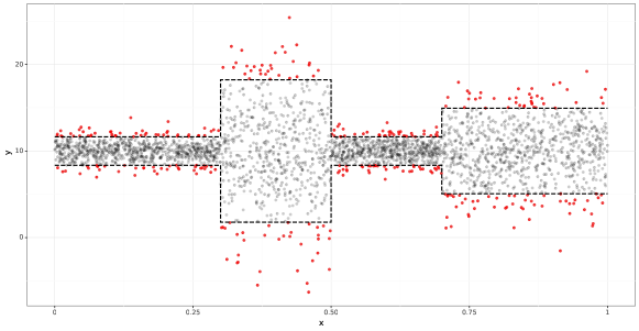
Figure 1: Simulated Train Dataset with 7,000 observations $y\sim\mathcal{N}(10,(1+4(0.3<x<0.5)+2(x>0.7))$. Points outside the 5% and 95% quantile are coloured in red. The black dashed lines depict the actual 5% and 95% quantiles. Besides the only informative predictor $x$, we have added $X_{1},\ldots,X_{10}$ as noise variables.

As splitting procedures, that are internally used to construct trees, can detect changes in the mean only, standard tree-based implementations are not able to recognize any distributional changes (e.g., change of variance), even if these can be related to covariates (Hothorn and Zeileis,, 2021). As such, basic versions of XGBoost and LightGBM don’t provide a way to model the full predictive distribution $F_{Y}(y|\mathbf{x})$, as they focus on predicting the conditional mean $\mathbb{E}(Y|\mathbf{X}=\mathbf{x})$ only.

In general, the syntax of our DGBM models is similar to the original XGBoost and LightGBM implementations. However, the user has to make a distributional assumption for GBMLSS by specifying a family in the function call, as well as to specify the order of the Bernstein-Polynomial $M$ for NFBoost. Since the data have been generated by a Normal distribution, we use the Normal as an input for GBMLSS. For NFBoost, we set $M=6$. Since our framework is likelihood-based, we can use unconditional density and CDF estimates to compare and evaluate the distributional fit prior to estimating the models. Figure 2 shows that the Bernstein-Polynomials slightly better capture the kurtotic shape of the data compared to the Normal assumption.

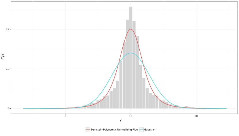
(a) Unconditional Density Plot

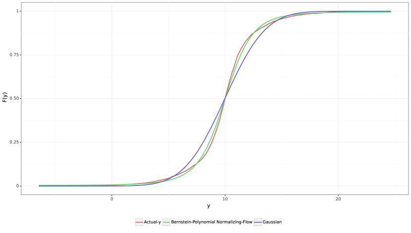
(b) Unconditional CDF Plot

Figure 2: Unconditional density and CDF plots of the Gaussian and Bernstein-Polynomial Normalizing-Flow.

The ability of the Bernstein-Polynomial Flow to better approximate the data is also confirmed by the likelihood comparison shown in Table 1.

Distribution	NLL
Gaussian	6.9935
Bernstein-Polynomial Normalizing-Flow ($M$=6)	2.3688

TABLE 1: NegLogLikelihood Comparison of Gaussian and Bernstein-Polynomial Normalizing-Flow

When fitting both models, the user has the option of providing a list of hyper-parameters to find an optimized set of parameters using Optuna of Akiba et al., (2019). Once the model is trained, we obtain prediction intervals and quantiles of interest directly from the predicted distribution. Figure 3 shows the predictions of the DGBM models for the 5% and 95% quantile in blue.

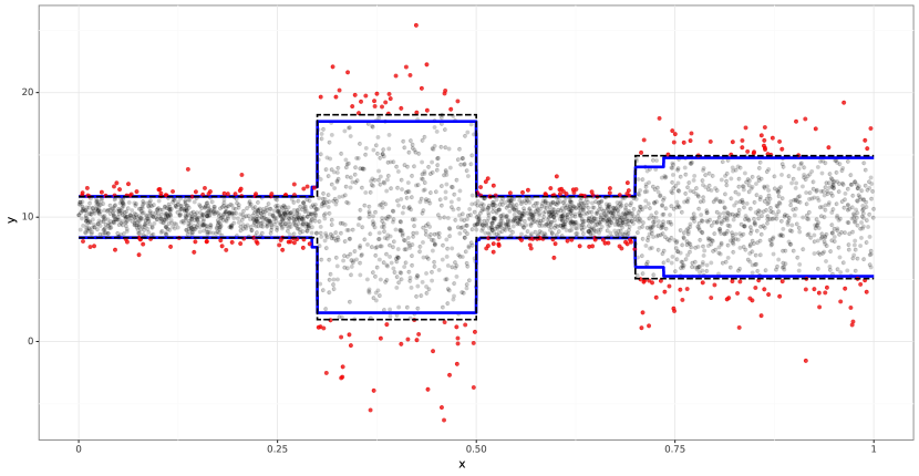
(a) GBMLSS-XGB

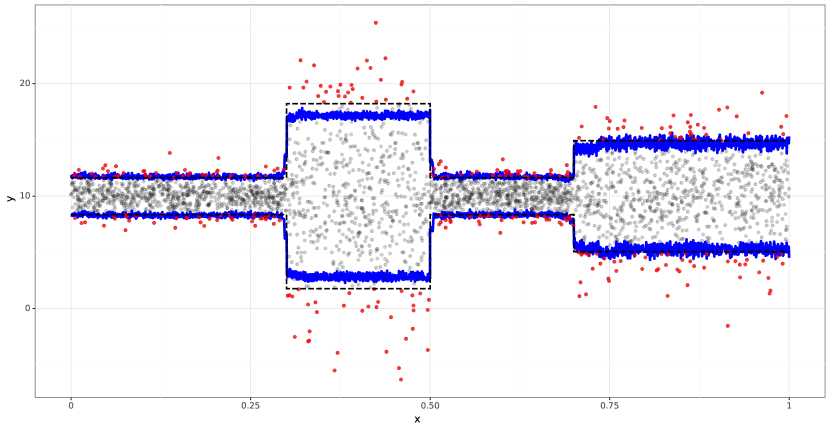
(b) GBMLSS-LGB

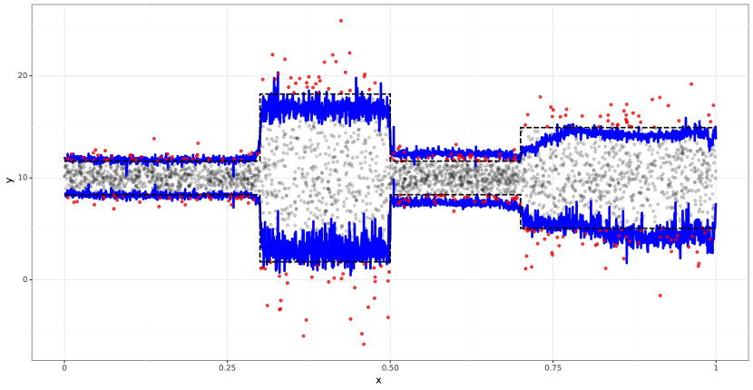
(c) NFBoost-XGB

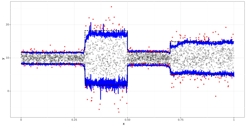
(d) NFBoost-LGB

Figure 3: Simulated Test Dataset with 3,000 observations $y\sim\mathcal{N}(10,(1+4(0.3<x<0.5)+2(x>0.7))$. Points outside the conditional 5% and 95% quantile are in red. The black dashed lines depict the actual 5% and 95% quantiles. Conditional 5% and 95% quantile predictions obtained from the DGBM models are depicted by the blue lines. Besides the only informative predictor $x$, we have added $X_{1},\ldots,X_{10}$ as noise variables.

Investigation of Figure 3 shows that all models in our DGBM framework correctly estimate the heteroskedasticity in the data. The top panels of Figure 3 further show that GBMLSS predictions of the 5% and 95% quantiles are less variable and show a higher alignment with the theoretical quantiles. The difference in the level of variability between NFBoost and GBMLSS predictions becomes most apparent when comparing Panel 3(a) with Panel 3(c): while both models use XGBoost as a computational engine, Panel 3(c) shows a much higher variability of the predicted quantiles. However, comparing Panel 3(c) with Panel 3(d) also shows that while using the same polynomial order $M$, LightGBM predictions exhibit less variability. One reason might be that a parametric distributional assumption with less parameters to estimate leads to a more stable prediction: for the Gaussian, the GBMLSS models need to estimate 2 parameters only, whereas for the Normalizing-Flow based models, $M+$4 parameters need to be estimated. Its smooth approximation of the theoretical quantiles shown in Panel 3(c) also indicates that GBMLSS-XGB profits the most from the unconditional parameter initialization: while all other models iterate to, or close to the maximum number of 500 boosting rounds for all hyper-parameter combinations, GBMLSS-XGB stops already early after 25 iterations.

Our GBMLSS models also provide insights into the data generating process via feature importances and partial dependence plots for all distributional parameters. Since the conditional mean is simulated as being constant, Figure 4 displays the effect on the conditional variance $\mathbb{V}(Y|\mathbf{X}=\mathbf{x})$ only.

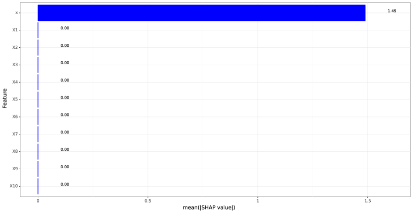
(a) GBMLSS-XGB Feature Importance

(b) GBMLSS-XGB Partial Dependence Plot

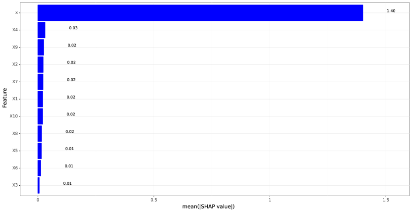
(c) GBMLSS-LGB Feature Importance

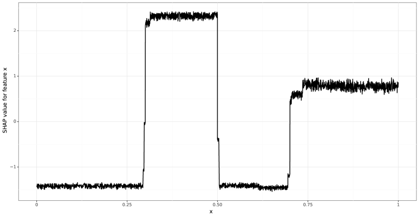
(d) GBMLSS-LGB Partial Dependence Plot

Figure 4: Feature importance and partial dependence plots using Shapley Values.

The top panels of Figure 4 show that all GBMLSS models correctly identify the only informative predictor $x$ and do not consider any of the noise variables $X_{1},\ldots,X_{10}$ as important features. The partial dependence plots in the right panels of Figure 4 also show that both models correctly identify the shape and magnitude of the heteroskedasticity in the data. As already suggested by the predicted quantiles shown in Figure 3, Panels 4(b) and 4(d) confirm that the conditional variance estimate of GBMLSS-XGB appears to be less variable compared to the GBMLSS-LGB estimate.

IV-B UCI Regression Datasets

In this section, we benchmark our DGBM framework against NGBoost (Duan et al.,, 2020) and PGBM (Sprangers et al.,, 2021) using a subset of the UCI-datasets of Dua and Graff, (2017). For conducting the experiments, we proceed as follows: for each dataset, we create 5 randomly shuffled folds and split each fold into train and test, where we keep 10% of the data for evaluating the models and use the remaining 90% for training. To make the results comparable to Sprangers et al., (2021); Duan et al., (2020), we assume a Gaussian distribution for all parametric distributional models and keep the set of hyper-parameters constant across all datasets. As such, neither early stopping nor hyper-parameter tuning is used during the experiments. All models are trained based on 1,000 boosting rounds. Table 2 summarises the hyper-parameters used for conducting the experiments.

	GBMLSS-LGB	GBMLSS-XGB	NFBoost-LGB	NFBoost-XGB	NGBoost	PGBM
min_split_gain (gamma)	0	0	0	0	0	0
min_data_in_leaf	1	1	1	1	1	1
min_data_in_bin	1	na	1	na	na	na
max_bin	64	64	64	64	na	64
max_leaves	16	16	16	16	na	16
max_depth	-1	0	-1	0	3	-1
learning_rate	0.1	0.1	0.01/0.03	0.01/0.03	0.01	0.1
boosting_rounds	1,000	1,000	1,000	1,000	1,000	1,000
n_data_folds	5	5	5	5	5	5
lambda (alpha)	1.0	1.0	1.0	1.0	na	1.0
Bernstein-Order $M$ / Distribution	Gaussian	Gaussian	{10, 4, 8, 4, 10, 3}	{10, 4, 8, 4, 10, 3}	Gaussian	Gaussian

• For the yacht dataset, we log-transform the response and increase the learning rate of all NFBoost models from 0.01 to 0.03. To stabilize estimation of gradients and hessians, we scale all responses $y/100$. The table only shows hyper-parameter settings that deviate from default values. To use similar settings for both XGB and LGB models, we set $tree\_method=hist$ and $grow\_policy=lossguide$ for XGB based models. The dataset order of Bernstein-Polynomials $M$ is {boston, concrete, kin8nm, naval, protein, yacht}.

TABLE 2: Hyper-Parameters for UCI-dataset experiments

Probabilistic forecasts of all models are evaluated using the Continuous Ranked Probability Score (CRPS) of Gneiting and Raftery, (2007), which is a measure of the difference between the predicted and the empirical cumulative distribution function of the ground-truth observation $y$

$$CRPS(F,y)=\int_{\mathbb{R}}\big{(}F(z)-\mathds{I}\{y\leq z\}\big{)}^{2}dz$$ (9)

where $\mathds{I}\{y\leq z\}$ denotes the indicator function. The CRPS is a proper scoring function that attains a minimum if the predicted distribution $F$ and the data distribution are identical. To evaluate all models, we use 1,000 samples drawn from the predicted distributions.

To determine the order of the Bernstein-Polynomial, we search over the grid $M\in[3,10]$ and select the order with the lowest negative log-likelihood. We want to stress that the selection of $M$ is crucial since it determines the flexibility of the estimated cumulative distribution function. In fact, very low and very high orders of $M$ represent two different extremes: for $M$=1 and $F_{Z}=N(0,1)$, $\hat{F}_{Y}$ belongs to the family of Gaussian distribution functions, whereas for $M=n-1$, $\hat{F}_{Y}$ constitutes an interpolation of the data. Therefore, since Bernstein-Polynomial Flows can approximate distribution functions of exquisite complexity for high $M$, an appropriate choice of $M$ is crucial to maintain a balance between a good approximation and the ability of the model to extrapolate beyond unseen data.

Before we present the results of the experiments, we investigate Figure 5 that shows unconditional density plots of the Gaussian and Bernstein-Polynomial Normalizing-Flow for the UCI-Datasets.

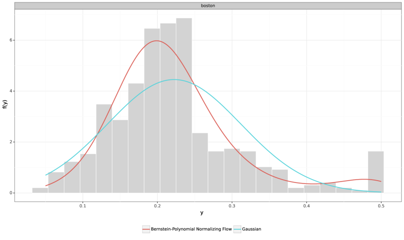
(a)

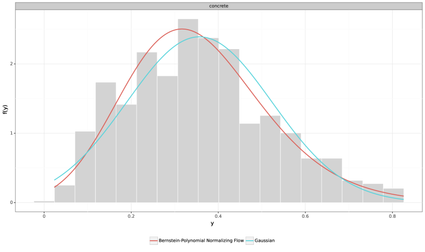
(b)

(c)

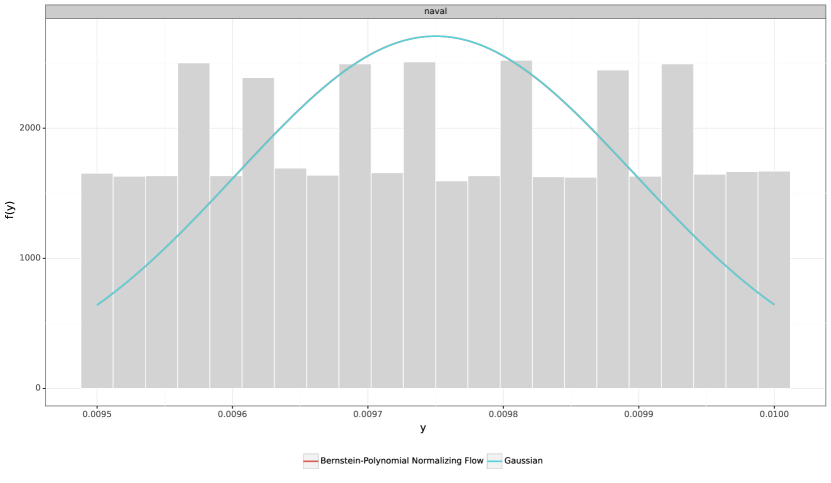
(d)

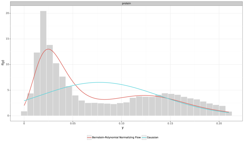
(e)

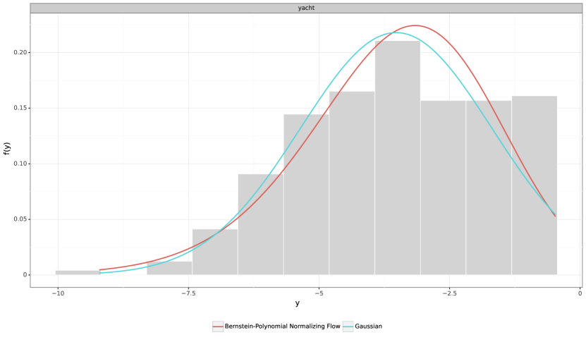
(f)

Figure 5: Unconditional density plots of the Gaussian and Bernstein-Polynomial Normalizing-Flow for the UCI-Datasets.

The ability of the Bernstein-Polynomial Flow to reconstruct any data-generating process is most evident from Panel 5(e), where we expect the NFBoost models to have a higher accuracy than parametric distribution models, since the protein dataset exhibits a bimodal behaviour that is not well captured by the Gaussian. We now turn to the discussion of the CRPS scores presented in Table 3.

	GBMLSS-LGB	GBMLSS-XGB	NFBoost-LGB	NFBoost-XGB	NGBoost	PGBM
boston (N=506)	1.6935 [1.5855, 1.73]	1.6153 [1.5198, 1.629]	1.9368 [1.6219, 2.0662]	1.5549 [1.5537, 1.5746]	1.7007 [1.6143, 1.8061]	1.5715 [1.5664, 1.5991]
concrete (N=1,030)	1.6172 [1.5444, 1.7071]	1.642 [1.5611, 1.8968]	2.1467 [1.9287, 2.2436]	2.3532 [2.0562, 2.3712]	2.5161 [2.3637, 2.682]	1.8121 [1.6745, 2.2021]
kin8nm (N=8,192)	0.0729 [0.0728, 0.073]	0.073 [0.0724, 0.0731]	0.0629 [0.0625, 0.0632]	0.0639 [0.0625, 0.0641]	0.0965 [0.0941, 0.0968]	0.1401 [0.1396, 0.195]
naval (N=11,934)	0.0034 [0.0034, 0.0034]	0.0034 [0.0034, 0.0034]	0.0035 [0.0035, 0.0035]	0.0035 [0.0035, 0.0035]	0.0017 [0.0017, 0.0018]	0.0061 [0.0057, 0.0069]
protein (N=45,730)	1.9898 [1.9839, 2.0063]	1.9974 [1.9869, 2.0034]	1.9031 [1.8861, 1.9203]	1.935 [1.9245, 1.9378]	2.5259 [2.5131, 2.5262]	2.1103 [2.1085, 2.1734]
yacht (N=308)	5.7119 [5.3285, 7.1834]	7.3127 [3.6087, 7.9982]	10.655 [10.4204, 11.3639]	25.0991 [22.4859, 25.8206]	6.1083 [5.6999, 7.4556]	14.877 [14.1427, 19.3816]

• The table shows median CRPS scores across all folds, with interquartile-range values in parentheses, i.e., $q_{0.5}(q_{0.25},q_{0.75})$. Lower is better, with best results in bold.

TABLE 3: CRPS scores across models and UCI datasets

As hypothesized earlier, Normalizing-Flow based models outperform parametric distributional models for the bimodal protein dataset due to their higher flexibility. A similar picture emerges for the slightly skewed and kurtotic boston dataset, where NFBoost-XGB achieves the highest accuracy, closely followed by the PGBM model. The comparatively small number of observations in the boston data set, however, may account for the unstable behaviour of NFBoost-LGB. From Table 3 it also appears that for small and medium sized datasets, such as the concrete, where a parametric Gaussian distribution is a reasonable approximation to the data, parametric GBMLSS models are more efficient and provide a higher accuracy than Normalizing-Flow based models. Even though the kin8nm data are also well described by a Gaussian, we attribute the higher accuracy of NFBoost models to the number of observations and hence to the higher informational content in the data, which allows more flexible Flow-based models to be estimated. For the smallest yacht dataset, NFBoost-XGB appears to have the most difficulties, possibly due to the small amount of observations relative to the number of features and parameters being estimated. For the uniformly distributed naval dataset, NGBoost achieves the lowest score, with all models of our DGBM framework scoring equally.

We also report CRPS ranks in Table 4, showing that all models in our DGBM framework achieve state-of-the-art accuracy. Among the DGBM models, GBMLSS achieve the highest accuracy, with GBMLSS-LGB ranking best on average. For the NFBoost models, NFBoost-XGB has a small lead over NFBoost-LGB.

	GBMLSS-LGB	GBMLSS-XGB	NFBoost-LGB	NFBoost-XGB	NGBoost	PGBM
boston (N=506)	4	3	6	1	5	2
concrete (N=1,030)	1	2	4	5	6	3
kin8nm (N=8,192)	3	4	1	2	5	6
naval (N=11,934)	3	2	5	4	1	6
protein (N=45,730)	3	4	1	2	6	5
yacht (N=308)	1	3	4	6	2	5
Average Rank	2.5	3.0	3.5	3.3	4.2	4.5

• Results are ranks based on median CRPS scores reported in Table 3. Lower is better.

TABLE 4: CRPS score rankings for the UCI datasets

In addition to CRPS metrics, runtimes for all models are presented in Table 5.

	GBMLSS-LGB	GBMLSS-XGB	NFBoost-LGB	NFBoost-XGB	NGBoost	PGBM
boston (N=506)	0.0246	0.0436	4.4566	4.7024	0.1166	0.0450
concrete (N=1,030)	0.0206	0.0656	4.8334	5.1640	0.1208	0.0437
kin8nm (N=8,192	0.0432	0.3541	7.2432	7.6311	0.6378	0.1047
naval (N=11,934)	0.0535	0.5101	5.2801	5.9496	1.0536	0.1560
protein (N=45,730)	0.1401	1.8121	25.8645	31.7632	3.5939	0.4536
yacht (N=308)	0.0164	0.0347	3.9868	3.9612	0.0927	0.0391
Average Rank	1.0	2.7	5.2	5.8	4.0	2.3

• Results are runtimes in minutes, averaged across all folds. Lower is better, with minimum runtime in bold. The bottom part shows the runtime rank averaged across all datasets.

TABLE 5: Average runtime in minutes

Combining CRPS scores and runtime ranks of Table 5 shows that GBMLSS-LGB is not only the fastest, but also the most accurate model on the benchmark datasets, with PGBM being close second. This corresponds with the findings of the M5 forecasting competition, where LightGBM consistently scores high, both for the point and probabilistic competitions. However, Table 5 also shows that runtimes for NFBoost models are not yet competitive, constantly exceeding those of other approaches by several orders of magnitude, especially for larger datasets such as the protein. Since the analysis and efficiency improvements are still ongoing, we can only formulate some mild hypotheses about the reasons for the runtime issue at this stage. One reason might be the known fact that XGBoost and LightGBM scale $\mathcal{O}(P^{2})$ with the number of parameters $P$, where a separate tree is grown for each parameter. To achieve a flexible approximation to the data, the order of the Bernstein-Polynomial $M$ needs to be reasonably high. As for the protein that shows the highest runtime, we use $P=M(10)+4$ parameters which requires the NFBoost models to estimate 7 times as many parameters compared to GBMLSS models. Another reason might be that NFBoost models rely on a set of TensorFlow functions that require many intermediate results to be shuffled back and forth between tensors and arrays. This can induce a significant latency, which in turn increases runtime. Furthermore, while all other models use exact gradients and hessians, NFBoost relies on automatic differentiation as an approximation. Although this greatly enhances the variety of loss functions available for model training, it might also have a negative effect on runtime. From experiments we have conducted so far it appears that the automatic derivation of the hessian poses a significant computational bottleneck. To circumvent approximating the second-order derivative, we also trained models in which the hessian was set to 1. However, this generally resulted in lower accuracy, which is consistent with the results reported by Sigrist, (2021).

V Conclusion, Limitations and Future Research

’Practitioners expect forecasting to reduce future uncertainty by providing accurate predictions like those in hard sciences. However, this is a great misconception. A major purpose of forecasting is not to reduce uncertainty but reveal its full extent and implications by estimating it as precisely as possible. [$\ldots$] The challenge for the forecasting field is how to persuade practitioners of the reality that all forecasts are uncertain and that this uncertainty cannot be ignored, as doing so could lead to catastrophic consequences.’ (Makridakis et al., 2021b, )

The language of statistics and machine learning is of probabilistic nature. Instead of a single point forecast only, distributional modelling provides a range of outcomes and the probability of each of those occurring. Consequently, any model that falls short of providing quantification of the uncertainty attached to its outcome is likely to yield an incomplete and potentially misleading picture. In an effort to obtain probabilistic forecasts from tree-based models, this paper presents a unified distributional gradient boosting framework for regression tasks that allows one to either model all conditional moments of a parametric distribution, or to approximate the conditional cumulative distribution function via Normalizing Flows. Based on a simulation study and real-world data examples, we have demonstrated our framework to be competitive to existing approaches and that Normalizing Flow based modelling of the conditional cumulative distribution function is superior in cases where the data cannot be described well using parametric distributions. Furthermore, our results suggest that the effectiveness of our Normalizing-Flow based tree-models tends to increase with data size.

Despite its flexibility, we acknowledge some limitations of our framework that require additional research. Even though distributional modelling relaxes the assumption of observations being identically distributed, tree-based models are not yet able to explicitly incorporate dependencies between observations, e.g., time, longitudinal or space. While features that represent, e.g., time, can be manually engineered, most tree-based models in their current implementation, however, are not able to infer these dependencies in the data themselves without appropriate changes of the estimation process. This contrasts with, for example, deep RNN models that are designed to model sequential data more naturally. Hence, a future extension of our approach would be to directly model longitudinal or temporal dependencies as part of the training process, as discussed in, e.g., Sela and Simonoff, (2012); Hajjem et al., (2011). Another interesting extension of distributional modelling, as proposed by O’Malley et al., (2021); Klein et al., (2022); Marra and Radice, (2017); Klein and Kneib, (2016), is to extend the univariate case to a multiple response setting, with several responses of interest that are potentially interdependent. Also, since our framework relies on multi-parameter optimization, where a separate tree is grown for each parameter, estimating many parameters for a large dataset can become computationally expensive, especially for NFBoost, where $M$ Bernstein-Polynomials in addition to 4 scale and shift parameters need to be estimated. For the time being, we leave a more runtime efficient version of our framework to future implementation and research. Finally, we consider the extension of our framework to allow for other Normalizing Flow types, suitable for count or ordinal data as proposed by Kook et al., (2021), as an interesting enhancement.

References

- Abadi et al., (2015) Abadi, M., Agarwal, A., Barham, P., Brevdo, E., Chen, Z., Citro, C., Corrado, G. S., Davis, A., Dean, J., Devin, M., Ghemawat, S., Goodfellow, I., Harp, A., Irving, G., Isard, M., Jia, Y., Jozefowicz, R., Kaiser, L., Kudlur, M., Levenberg, J., Mané, D., Monga, R., Moore, S., Murray, D., Olah, C., Schuster, M., Shlens, J., Steiner, B., Sutskever, I., Talwar, K., Tucker, P., Vanhoucke, V., Vasudevan, V., Viégas, F., Vinyals, O., Warden, P., Wattenberg, M., Wicke, M., Yu, Y., and Zheng, X. (2015). TensorFlow: Large-Scale Machine Learning on Heterogeneous Systems.
- Akiba et al., (2019) Akiba, T., Sano, S., Yanase, T., Ohta, T., and Koyama, M. (2019). Optuna: A Next-generation Hyperparameter Optimization Framework. In Teredesai, A., editor, Proceedings of the 25th ACM SIGKDD International Conference on Knowledge Discovery & Data Mining, ACM Digital Library, pages 2623–2631, New York,NY,United States. Association for Computing Machinery.
- Arpogaus, (2022) Arpogaus, M. (2022). Short-Term Probabilistic Load Forecasting using Conditioned Bernstein-Polynomial Normalizing Flows.
- Arpogaus et al., (2021) Arpogaus, M., Voss, M., Sick, B., Nigge-Uricher, M., and Dürr, O. (2021). Probabilistic Short-Term Low-Voltage Load Forecasting using Bernstein-Polynomial Normalizing Flows. In ICML 2021, Workshop Tackling Climate Change with Machine Learning, June 26, 2021, virtual.
- Athey et al., (2019) Athey, S., Tibshirani, J., and Wager, S. (2019). Generalized random forests. The Annals of Statistics, 47(2):1148–1178.
- Baumann et al., (2021) Baumann, P. F. M., Hothorn, T., and Rügamer, D. (2021). Deep Conditional Transformation Models. In Oliver, N., Perez Cruz, F., Kramer, S., Read, J., and Lozano, J. A., editors, Research Track, volume 12977 of Lecture Notes in Artificial Intelligence, pages 3–18. Springer, Cham.
- Chen and Guestrin, (2016) Chen, T. and Guestrin, C. (2016). XGBoost: A Scalable Tree Boosting System. In Proceedings of the 22nd ACM SIGKDD International Conference on Knowledge Discovery and Data Mining, KDD ’16, pages 785–794, New York, NY, USA. Association for Computing Machinery.
- Chipman et al., (2010) Chipman, H. A., George, E. I., and McCulloch, R. E. (2010). BART: Bayesian additive regression trees. The Annals of Applied Statistics, 4(1):266–298.
- Dua and Graff, (2017) Dua, D. and Graff, C. (2017). UCI Machine Learning Repository.
- Duan et al., (2020) Duan, T., Anand, A., Ding, D. Y., Thai, K. K., Basu, S., Ng, A. Y., and Schuler, A. (2020). NGBoost: Natural Gradient Boosting for Probabilistic Prediction. In Proceedings of the 37th International Conference on Machine Learning, ICML 2020, 13-18 July 2020, Virtual Event, volume 119 of Proceedings of Machine Learning Research, pages 2690–2700. PMLR.
- Dürr et al., (2022) Dürr, O., Hörling, S., Dold, D., Kovylov, I., and Sick, B. (2022). Bernstein Flows for Flexible Posteriors in Variational Bayes. arXiv Pre-Print, pages 1–18.
- Fahrmeir and Kneib, (2011) Fahrmeir, L. and Kneib, T. (2011). Bayesian smoothing and regression for longitudinal, spatial and event history data, volume 36 of Oxford statistical science series. Oxford University Press, Oxford and New York.
- Fahrmeir et al., (2013) Fahrmeir, L., Kneib, T., Lang, S., and Marx, B. (2013). Regression: Models, methods and applications. Springer, Berlin, 1 edition.
- Farouki, (2012) Farouki, R. T. (2012). The Bernstein polynomial basis: A centennial retrospective. Computer Aided Geometric Design, 29(6):379–419.
- Friedman, (2020) Friedman, J. H. (2020). Contrast trees and distribution boosting. Proceedings of the National Academy of Sciences, 117(35):21175–21184.
- Gasthaus et al., (2019) Gasthaus, J., Benidis, K., Wang, Y., Rangapuram, S. S., Salinas, D., Flunkert, V., and Januschowski, T. (2019). Probabilistic Forecasting with Spline Quantile Function RNNs. In Chaudhuri, K. and Sugiyama, M., editors, Proceedings of the Twenty-Second International Conference on Artificial Intelligence and Statistics, volume 89 of Proceedings of Machine Learning Research, pages 1901–1910. PMLR.
- Giaquinto and Banerjee, (2020) Giaquinto, R. and Banerjee, A. (2020). Gradient Boosted Normalizing Flows. In H. Larochelle, M. Ranzato, R. Hadsell, M. F. Balcan, and H. Lin, editors, Advances in Neural Information Processing Systems, volume 33, pages 22104–22117. Curran Associates, Inc.
- Glorot and Bengio, (2010) Glorot, X. and Bengio, Y. (2010). Understanding the difficulty of training deep feedforward neural networks. In Teh, Y. W. and Titterington, M., editors, Proceedings of the Thirteenth International Conference on Artificial Intelligence and Statistics, volume 9 of Proceedings of Machine Learning Research, pages 249–256, Chia Laguna Resort, Sardinia, Italy. PMLR.
- Gneiting and Raftery, (2007) Gneiting, T. and Raftery, A. E. (2007). Strictly proper scoring rules, prediction, and estimation. Journal of the American Statistical Association, 102(477):359–378.
- Hajjem et al., (2011) Hajjem, A., Bellavance, F., and Larocque, D. (2011). Mixed effects regression trees for clustered data. Statistics & Probability Letters, 81(4):451–459.
- Hasson et al., (2021) Hasson, H., Wang, B., Januschowski, T., and Gasthaus, J. (2021). Probabilistic Forecasting: A Level-Set Approach. In Beygelzimer, A., Dauphin, Y., Liang, P., and Wortman Vaughan, J., editors, Advances in Neural Information Processing Systems.
- He et al., (2015) He, K., Zhang, X., Ren, S., and Sun, J. (2015). Delving Deep into Rectifiers: Surpassing Human-Level Performance on ImageNet Classification. 2015 IEEE International Conference on Computer Vision (ICCV), pages 1026–1034.
- Hothorn, (2020) Hothorn, T. (2020). Transformation Boosting Machines. Statistics and Computing, 30(1):141–152.
- Hothorn et al., (2014) Hothorn, T., Kneib, T., and Bühlmann, P. (2014). Conditional transformation models. Journal of the Royal Statistical Society: Series B (Statistical Methodology), 76(1):3–27.
- Hothorn and Zeileis, (2021) Hothorn, T. and Zeileis, A. (2021). Predictive Distribution Modeling Using Transformation Forests. Journal of Computational and Graphical Statistics, 30(4):1181–1196.
- Hüllermeier and Waegeman, (2021) Hüllermeier, E. and Waegeman, W. (2021). Aleatoric and epistemic uncertainty in machine learning: an introduction to concepts and methods. Machine Learning, 110(3):457–506.
- Januschowski et al., (2020) Januschowski, T., Gasthaus, J., Wang, Y., Salinas, D., Flunkert, V., Bohlke-Schneider, M., and Callot, L. (2020). Criteria for classifying forecasting methods. International Journal of Forecasting, 36(1):167–177.
- Januschowski and Kolassa, (2019) Januschowski, T. and Kolassa, S. (2019). A classification of business forecasting problems. Foresight: The International Journal of Applied Forecasting, 52:36–43.
- Januschowski et al., (2021) Januschowski, T., Wang, Y., Torkkola, K., Erkkilä, T., Hasson, H., and Gasthaus, J. (2021). Forecasting with trees. International Journal of Forecasting.
- Ke et al., (2017) Ke, G., Meng, Q., Finley, T., Wang, T., Chen, W., Ma, W., Ye, Q., and Liu, T.-Y. (2017). LightGBM: A Highly Efficient Gradient Boosting Decision Tree. In Proceedings of the 31st International Conference on Neural Information Processing Systems, NIPS’17, pages 3149–3157, Red Hook, NY, USA. Curran Associates Inc.
- Klein et al., (2022) Klein, N., Hothorn, T., Barbanti, L., and Kneib, T. (2022). Multivariate conditional transformation models. Scandinavian Journal of Statistics, 49(1):116–142.
- Klein and Kneib, (2016) Klein, N. and Kneib, T. (2016). Simultaneous inference in structured additive conditional copula regression models: a unifying Bayesian approach. Statistics and Computing, 26(4):841–860.
- (33) Klein, N., Kneib, T., and Lang, S. (2015a). Bayesian Generalized Additive Models for Location, Scale, and Shape for Zero-Inflated and Overdispersed Count Data. Journal of the American Statistical Association, 110(509):405–419.
- (34) Klein, N., Kneib, T., Lang, S., and Sohn, A. (2015b). Bayesian structured additive distributional regression with an application to regional income inequality in Germany. The Annals of Applied Statistics, 9(2):1024–1052.
- Kobyzev et al., (2020) Kobyzev, I., Prince, S., and Brubaker, M. (2020). Normalizing Flows: An Introduction and Review of Current Methods. IEEE Transactions on Pattern Analysis and Machine Intelligence, PP:1.
- Koenker and Bassett, (1978) Koenker, R. and Bassett, G. (1978). Regression Quantiles. Econometrica, 46(1):33–50.
- Kook et al., (2021) Kook, L., Herzog, L., Hothorn, T., Dürr, O., and Sick, B. (2021). Deep and interpretable regression models for ordinal outcomes. arXiv Pre-Print, pages 1–41.
- Kurle et al., (2020) Kurle, R., Rangapuram, S. S., de Bézenac, E., Günnemann, S., and Gasthaus, J. (2020). Deep Rao-Blackwellised Particle Filters for Time Series Forecasting. In H. Larochelle, M. Ranzato, R. Hadsell, M. F. Balcan, and H. Lin, editors, Advances in Neural Information Processing Systems, volume 33, pages 15371–15382. Curran Associates, Inc.
- Lundberg et al., (2020) Lundberg, S. M., Erion, G., Chen, H., DeGrave, A., Prutkin, J. M., Nair, B., Katz, R., Himmelfarb, J., Bansal, N., and Lee, S.-I. (2020). From local explanations to global understanding with explainable AI for trees. Nature Machine Intelligence, 2(1):2522–5839.
- Lundberg and Lee, (2017) Lundberg, S. M. and Lee, S.-I. (2017). A Unified Approach to Interpreting Model Predictions. In I. Guyon, U. V. Luxburg, S. Bengio, H. Wallach, R. Fergus, S. Vishwanathan, and R. Garnett, editors, Advances in Neural Information Processing Systems 30, pages 4765–4774. Curran Associates, Inc.
- (41) Makridakis, S., Spiliotis, E., and Assimakopoulos, V. (2021a). The M5 competition: Background, organization, and implementation. International Journal of Forecasting.
- (42) Makridakis, S., Spiliotis, E., Assimakopoulos, V., Chen, Z., Gaba, A., Tsetlin, I., and Winkler, R. L. (2021b). The M5 uncertainty competition: Results, findings and conclusions. International Journal of Forecasting.
- Marra and Radice, (2017) Marra, G. and Radice, R. (2017). Bivariate copula additive models for location, scale and shape. Computational Statistics & Data Analysis, 112:99–113.
- März, (2019) März, A. (2019). XGBoostLSS - An extension of XGBoost to probabilistic forecasting. arXiv Pre-Print, pages 1–23.
- März, (2020) März, A. (2020). CatBoostLSS - An extension of CatBoost to probabilistic forecasting. arXiv Pre-Print, pages 1–18.
- Meinshausen, (2006) Meinshausen, N. (2006). Quantile Regression Forests. Journal of Machine Learning Research, 7(35):983–999.
- O’Malley et al., (2021) O’Malley, M., Sykulski, A. M., Lumpkin, R., and Schuler, A. (2021). Multivariate Probabilistic Regression with Natural Gradient Boosting. arXiv Pre-Print, pages 1–19.
- Papamakarios et al., (2021) Papamakarios, G., Nalisnick, E. T., Rezende, D. J., Mohamed, S., and Lakshminarayanan, B. (2021). Normalizing Flows for Probabilistic Modeling and Inference. Journal of Machine Learning Research, 22:1–64.
- Paszke et al., (2019) Paszke, A., Gross, S., Massa, F., Lerer, A., Bradbury, J., Chanan, G., Killeen, T., Lin, Z., Gimelshein, N., Antiga, L., Desmaison, A., Köpf, A., Yang, E., DeVito, Z., Raison, M., Tejani, A., Chilamkurthy, S., Steiner, B., Fang, L., Bai, J., and Chintala, S. (2019). PyTorch: An Imperative Style, High-Performance Deep Learning Library. In Proceedings of the 33rd International Conference on Neural Information Processing Systems. Curran Associates Inc, Red Hook, NY, USA.
- Pratola et al., (2020) Pratola, M. T., Chipman, H. A., George, E. I., and McCulloch, R. E. (2020). Heteroscedastic BART via Multiplicative Regression Trees. Journal of Computational and Graphical Statistics, 29(2):405–417.
- Rangapuram et al., (2021) Rangapuram, S. S., Werner, L. D., Benidis, K., Mercado, P., Gasthaus, J., and Januschowski, T. (2021). End-to-End Learning of Coherent Probabilistic Forecasts for Hierarchical Time Series. In Meila, M. and Zhang, T., editors, Proceedings of the 38th International Conference on Machine Learning, volume 139 of Proceedings of Machine Learning Research, pages 8832–8843. PMLR.
- Rasul et al., (2021) Rasul, K., Sheikh, A.-S., Schuster, I., Bergmann, U. M., and Vollgraf, R. (2021). Multivariate Probabilistic Time Series Forecasting via Conditioned Normalizing Flows. In International Conference on Learning Representations.
- Rigby and Stasinopoulos, (2005) Rigby, R. A. and Stasinopoulos, D. M. (2005). Generalized additive models for location, scale and shape. Journal of the Royal Statistical Society: Series C (Applied Statistics), 54(3):507–554.
- Rügamer et al., (2022) Rügamer, D., Baumann, P. F. M., Kneib, T., and Hothorn, T. (2022). Probabilistic Time Series Forecasts with Autoregressive Transformation Models. arXiv Pre-Print, pages 1–16.
- Salinas et al., (2020) Salinas, D., Flunkert, V., Gasthaus, J., and Januschowski, T. (2020). DeepAR: Probabilistic forecasting with autoregressive recurrent networks. International Journal of Forecasting, 36(3):1181–1191.
- Schlosser et al., (2018) Schlosser, L., Hothorn, T., Stauffer, R., and Zeileis, A. (2018). Distributional Regression Forests for Probabilistic Precipitation Forecasting in Complex Terrain. The Annals of Applied Statistics, 13(3):1564–1589.
- Sela and Simonoff, (2012) Sela, R. J. and Simonoff, J. S. (2012). RE-EM trees: a data mining approach for longitudinal and clustered data. Machine Learning, 86(2):169–207.
- Sick et al., (2021) Sick, B., Hothorn, T., and Dürr, O. (2021). Deep transformation models: Tackling complex regression problems with neural network based transformation models. In 2020 25th International Conference on Pattern Recognition (ICPR), pages 2476–2481.
- Sigrist, (2021) Sigrist, F. (2021). Gradient and Newton boosting for classification and regression. Expert Systems with Applications, 167:114080.
- Sprangers et al., (2021) Sprangers, O., Schelter, S., and de Rijke, M. (2021). Probabilistic Gradient Boosting Machines for Large-Scale Probabilistic Regression. In Proceedings of the 27th ACM SIGKDD Conference on Knowledge Discovery & Data Mining, KDD ’21, pages 1510–1520, New York, NY, USA. Association for Computing Machinery.
- Stasinopoulos et al., (2017) Stasinopoulos, M. D., Rigby, R. A., Heller, G. Z., Voudouris, V., and de Bastiani, F. (2017). Flexible Regression and Smoothing: Using GAMLSS in R. Chapman & Hall / CRC The R Series. CRC Press, London.
- Ziel, (2021) Ziel, F. (2021). M5 competition uncertainty: Overdispersion, distributional forecasting, GAMLSS, and beyond. International Journal of Forecasting.