Variational message passing for
online polynomial NARMAX identification

Abstract

We propose a variational Bayesian inference procedure for online nonlinear system identification. For each output observation, a set of parameter posterior distributions is updated, which is then used to form a posterior predictive distribution for future outputs. We focus on the class of polynomial NARMAX models, which we cast into probabilistic form and represent in terms of a Forney-style factor graph. Inference in this graph is efficiently performed by a variational message passing algorithm. We show empirically that our variational Bayesian estimator outperforms an online recursive least-squares estimator, most notably in small sample size settings and low noise regimes, and performs on par with an iterative least-squares estimator trained offline.

I Introduction

Nonlinear autoregressive moving-average with exogenous input (NARMAX) models are a staple in modern system identification. They have been applied to a wide range of systems such as the kinematics of mobile robots, the effects of space weather on earthbound electronics or the visual system of fruit flies [1]. We are interested in online estimators, because they allow for in-situ learning on embedded systems, and Bayesian estimators, i.e., posterior distributions instead of point estimates [2, 3]. The advantage of Bayesian estimators is that they are naturally robust to overfitting when data is still scarce [2, Ch. 5.3.1]. This paper proposes a recursive approximate Bayesian estimator for online system identification.

Despite its long history, Bayesian identification has always been challenging from a practical perspective [4]. Intractable integrals may prevent the formulation of an exact Bayesian estimator. Approximate Bayesian inference, especially Sequential Monte Carlo (a.k.a. particle filtering), has proven to be much more practical for dynamical systems [5]. Nonetheless, Monte Carlo-based methods are still quite computationally expensive. Variational Bayesian inference is an attractive alternative because it is typically much cheaper - computation-wise - than Monte Carlo sampling. The unnormalized posterior distribution function is approximated by minimizing a variational free energy functional with respect to a second probabilistic model [6]. The first uses of variational Bayes for system identification allowed for simultaneous estimation of states, coefficients and noise parameters in a wide range nonlinear stochastic differential equations [7, 8]. A particular technique called Dynamic Expectation Maximization (DEM), became popular and was recently used to simultaneously estimate not only states and inputs, but also colored noise [7, 9]. DEM relies on Laplace’s method, i.e., approximating the posterior with a Gaussian distribution using gradient-based techniques for finding the mode and local curvature. However, Laplace approximations fail for non-modal, multi-modal or discrete distributions, and can be inaccurate for distributions with higher-order moments (e.g., skewed or kurtotic ones). We employ a richer class of form constraints on the approximating distributions, namely the exponential family. A few recent papers have ventured into non-parametric families such as Gaussian processes and deep neural networks, achieving impressive results [10, 11]. But non-parametric models can quickly become computationally costly again. We formulate the inference procedure as message passing on a factor graph [12]. Computation can be distributed along nodes and edges by exploiting the factorization of the probabilistic model. This produces an efficient and parallelizable algorithm [13, 14]. Lastly, variational Bayes has found its way to autoregressive-based models. A recent ARMAX paper infers the noise sequence explicitly, but extending it to the nonlinear case is not trivial [15]. In addition, there are also NARX, NLARX, and SARX models which show competitive performance [16, 17, 18]. Our work complements these techniques by extending the scope to polynomial NARMAX models.

Our key contribution is the formulation of a recursive parameter and posterior predictive estimation algorithm using variational message passing on a Forney-style factor graph (Sec. IV-C). We show that our estimator competes well with an online least-squares estimator, outperforming it in small sample size settings without the need for informative priors (Sec. VI).

II NARMAX system

Consider a discrete-time dynamical system with an unknown time horizon, indexed by time $\in\mathbb{N}$. Let $u_{k}\in\mathbb{R}$ be a measured input signal, $y_{k}\in\mathbb{R}$ a measured output signal and $e_{k}\in\mathbb{R}$ be noise, drawn from a zero-mean Gaussian distribution with zero auto-correlation: $e_{k}\sim\mathcal{N}(0,\tau^{-1})$ where $\tau$ is a precision (inverse variance) parameter. In a NARMAX system, the output $y_{k}$ is generated according to:

$$y_{k}=f(u_{k},{\mathbf{u}}_{k-1},{\mathbf{y}}_{k-1},{\mathbf{e}}_{k-1})+e_{k}\,,$$ (1)

where ${\mathbf{u}}_{k-1}=(u_{k-1},..\,u_{k-M_{1}})$ is a vector containing $M_{1}$ delayed inputs, ${\mathbf{y}}_{k-1}=(y_{k-1},..\,y_{k-M_{2}})$ contains $M_{2}$ delayed outputs and the vector ${\mathbf{e}}_{k-1}=(e_{k-1},..\,e_{k-M_{3}})$ contains $M_{3}$ delayed noise instances. The function $f$ is assumed to be continuous, nonlinear, and time-invariant.

III Probabilistic Model

In a polynomial NARMAX, the function $f$ is modeled with a linear combination of coefficients $\theta$ and a polynomial basis function $\phi$ applied to inputs, outputs and errors:

$$y_{k}=\theta^{\top}\phi(u_{k},{\mathbf{u}}_{k-1},{\mathbf{y}}_{k-1},{\mathbf{e}}_{k-1})+e_{k}\,.$$ (2)

We define the vector $\phi_{k}=\phi(u_{k},{\mathbf{u}}_{k-1},{\mathbf{y}}_{k-1},{\mathbf{e}}_{k-1})$ for conciseness in later derivations. Specifying a probabilistic model consists of expressing the likelihood of observations, given parameters and noise, and posing a set of prior distributions for the unknown variables.

III-A Likelihood function

The noise variable is Gaussian distributed, which lets us express the likelihood of observing $y_{k}$ as:

$$p(y_{k}\>|\>u_{k},{\mathbf{u}}_{k\text{-}1},{\mathbf{y}}_{k\text{-}1},{\mathbf{e}}_{k\text{-}1},\theta,\tau)=\mathcal{N}\big{(}y_{k}\>|\>\theta^{\top}\phi_{k},\tau^{-1}\big{)}.$$ (3)

In this notation, it is implied that variables with subscripts smaller than $1$ drop out. So, the likelihood of the first observation simplifies to $p(y_{1}\>|\>u_{1},\theta,\tau)$. In practice, the vectors ${\mathbf{u}}_{k-1}$, ${\mathbf{y}}_{k-1}$, and ${\mathbf{e}}_{k-1}$ can be initialized with zeros and updated as data streams in. This allows for the recursive application of (3).

III-B Prior distributions

Our model has two unknown variables: the coefficients $\theta$ and the noise precision $\tau$. We need to pose an initial prior distribution for each. The coefficients are unbounded real-valued numbers, which could be modeled with a variety of continuous probability distributions. We choose a Gaussian distribution because its linear transformation $\theta^{\top}\phi_{k}$ results in another Gaussian that is conditionally conjugate to the likelihood function in (3) [2, Ch. 4.6]. The precision parameter $\tau$ is a strictly positive number, which could be modeled with for instance an Exponential or Gamma distribution. We choose a Gamma distribution, also because it is conditionally conjugate to our Gaussian likelihood [2, Ch. 4.6]. The initial priors are denoted as:

$$p(\theta)=\mathcal{N}\big{(}\theta\>|\>\mu_{0},\Lambda_{0}^{-1}\big{)}\,,\quad\ p(\tau)={\it\Gamma}\big{(}\tau\>|\>\alpha_{0},\beta_{0}\big{)}\,,$$ (4)

where the subscripts refer to time $k=0$, i.e., before $k=1$. We parameterize our Gaussian distributions with means $\mu$ and precision matrices $\Lambda$ (inverse covariance matrix) and our Gamma distributions with shapes $\alpha$ and rates $\beta$.

III-C Parameter posteriors

Given a likelihood function and prior distributions, we can apply Bayes’ rule to obtain posterior distributions. For the purposes of online system identification, we describe the posterior recursively [3, Chapter 3]. We start with the initial application of Bayes’ rule:

$$\underbrace{p(\theta,\tau\>|\>y_{1},u_{1})}_{\text{posterior at $k$=$1$}}=\underbrace{\frac{1}{p(y_{1}\>|\>u_{1})}}_{\text{evidence}}\underbrace{p(y_{1}\>|\>u_{1},\theta,\tau)}_{\text{likelihood}}\underbrace{p(\theta)p(\tau)}_{\text{initial priors}}.$$ (5)

The likelihood is multiplied with both priors to form a joint distribution over $y_{1}$, $\theta$ and $\tau$. That joint is normalized by the evidence for $y_{1}$, after which a joint posterior distribution for the parameters is obtained.

In recursive estimation, the posterior at one time point becomes the prior for the next [3]. At $k=2$, we have:

$$\underbrace{p(\theta,\tau\>|\>y_{1:2},u_{1:2},e_{1})}_{\text{posterior at $k$=$2$}}=\underbrace{\frac{1}{p(y_{2}\>|\>u_{1:2},y_{1},e_{1})}}_{\text{evidence for $y_{2}$}}$$

$$\ \qquad\qquad\cdot\underbrace{p(y_{2}\>|\>u_{1:2},y_{1},e_{1},\theta,\tau)}_{\text{likelihood of $y_{2}$}}\underbrace{p(\theta,\tau\>|\>y_{1},u_{1})}_{\text{prior (posterior $k$=$1$)}}\,.$$ (6)

The likelihood now contains the first elements of the previous input ${\mathbf{u}}_{k-1}$, output ${\mathbf{y}}_{k-1}$ and error ${\mathbf{e}}_{k-1}$ vectors. Note the structure of this equation: the previous posterior distribution is updated using two terms describing properties of the new observation $y_{2}$. In general, at time $k$, we have the following recursive posterior estimation procedure:

$$\underbrace{p(\theta,\tau|y_{1:k},u_{1:k},e_{1:k\text{-}1})}_{\text{parameter posterior at $k$}}=\frac{1}{\underbrace{p(y_{k}|u_{1:k},y_{1:k\text{-}1},e_{1:k\text{-}1})}_{\text{evidence}}}$$

$$\cdot\underbrace{p(y_{k}|u_{k},{\mathbf{u}}_{k\text{-}1},{\mathbf{y}}_{k\text{-}1},{\mathbf{e}}_{k\text{-}1},\theta,\tau)}_{\text{NARMAX likelihood}}\underbrace{p(\theta,\tau|y_{1:k\text{-}1},u_{1:k\text{-}1},e_{1:k\text{-}2})}_{\text{prior (posterior at $k\text{-}1$)}}\,,$$ (7)

where the evidence consists of integrating the product of the NARMAX likelihood and the prior with respect to the parameters $\theta$ and $\tau$:

$$p(y_{k}\>|\>u_{1:k},y_{1:k\text{-}1}, e_{1:k\text{-}1})=$$

$$\iint p(y_{k}\>|\>u_{k}, {\mathbf{u}}_{k\text{-}1},{\mathbf{y}}_{k\text{-}1},{\mathbf{e}}_{k\text{-}1},\theta,\tau)$$

$$\cdot p(\theta,\tau\>|\>y_{1:k\text{-}1},u_{1:k\text{-}1},e_{1:k\text{-}2})\ {\mathrm{d}}\theta{\mathrm{d}}\tau\,.$$ (8)

Unfortunately, the resulting posterior distribution is not of exactly the same form as the prior and is therefore not suited to recursive estimation. We approximate it with a more suitable distribution in Section IV.

III-D Posterior predictive

Given a posterior distribution of the parameters, the one-step-ahead posterior predictive distribution for the output is:

$$\underbrace{p(y_{k+1}\>|\>u_{1:k+1},y_{1:k},e_{1:k})}_{\text{posterior predictive}}=$$

$$\qquad\iint\underbrace{p(y_{k+1}\>|\>u_{k+1},{\mathbf{u}}_{k},{\mathbf{y}}_{k},{\mathbf{e}}_{k},\theta,\tau)}_{\text{likelihood of future observation}}$$

$$\qquad\qquad\qquad\qquad\quad\cdot\underbrace{p(\theta,\tau\>|\>y_{1:k},u_{1:k},e_{1:k\text{-}1})}_{\text{parameter posterior}}\mathrm{d}\theta\mathrm{d}\tau\,.$$ (9)

The posterior predictive is the average distribution for $y_{k+1}$, weighted by the posterior probability of each value of the parameters. This weighted average has a greater uncertainty than what would have obtained by plugging in a selected parameter. As such, the posterior predictive distribution is naturally regularized and is more robust to overfitting on the training data. Details on how to compute the posterior predictive are described in Section V.

III-E Prediction errors

Typically, the prediction errors are defined as the difference between the observed output $y_{k+1}$ and a numerical prediction $\hat{y}_{k+1}$ based on previous data [1]:

$$e_{k+1}=y_{k+1}-\hat{y}_{k+1}\,.$$ (10)

However, our prediction comes in the form of a posterior predictive distribution (i.e., a random variable, not a number). To adhere to the original definition of the prediction errors, we select the maximum a posteriori (MAP) of the posterior predictive distribution:

$$\hat{y}_{k+1}=\underset{y_{k+1}}{\arg\max}\ p(y_{k+1}\>|\>u_{1:k+1},y_{1:k},e_{1:k})\,.$$ (11)

To be clear, the order of operations in our recursive estimation procedure is as follows: at time $k$, we observe $y_{k}$ and update the parameter posterior according to (III-C). We then use the prediction $\hat{y}_{k}$ made during the previous time-step to compute the prediction error $e_{k}$. This error is used when we make a prediction for $\hat{y}_{k+1}$, which is passed on to the next time-step.

IV Inference

It is not possible to obtain the posterior distribution exactly due to the priors being merely conditionally conjugate and not jointly conjugate to our NARMAX likelihood. Below, we show how to approximate it in a recursive manner.

IV-A Free energy minimization

We adhere to a form of approximate Bayesian inference called variational free energy minimization [6]. Essentially, one poses a second probabilistic model $q$, called the recognition model, with which the generative model $p$ is approximated. The free energy functional at time $k$ is the Kullback-Leibler (KL) divergence between the recognition model and the true posterior, minus the log evidence:

$$\mathcal{F}_{k}[q_{k}]= \underbrace{\iint q_{k}(\theta,\tau)\ln\frac{q_{k}(\theta,\tau)}{p(\theta,\tau\>|\>y_{1:k},u_{1:k},e_{1:k\text{-}1})}{\mathrm{d}}\theta{\mathrm{d}}\tau}_{\text{approximation of posterior}}$$

$$\ \qquad-\ln\underbrace{p(y_{k}\>|\>u_{1:k},y_{1:k-1},e_{1:k\text{-}1})}_{\text{evidence}}\,.$$ (12)

Note that the $q_{k}$ that minimizes $\mathcal{F}_{k}$ is an optimal approximation of the true posterior at time $k$.

Equation (IV-A) necessitates the computation of the true posterior, which is intractable. We therefore re-formulate the objective along the lines of (III-C):

$$\mathcal{F}_{k}[q_{k}]=\!\underbrace{\iint q_{k}(\theta,\tau)\ln\frac{q_{k}(\theta,\tau)}{p(\theta,\tau|y_{1:k\text{-}1},u_{1:k\text{-}1},e_{1:k\text{-}2})}{\mathrm{d}}\theta{\mathrm{d}}\tau}_{\text{complexity}}$$

$$\!-\!\underbrace{\iint\!q_{k}(\theta,\tau)\ln p(y_{k}|u_{k},{\mathbf{u}}_{k\text{-}1},{\mathbf{y}}_{k\text{-}1},{\mathbf{e}}_{k\text{-}1},\theta,\tau){\mathrm{d}}\theta{\mathrm{d}}\tau}_{\text{accuracy}}.$$ (13)

Accuracy expresses how well the observation was predicted given the current parameter estimates and complexity is a measure of how much the recognition model deviates from the previous posterior. Minimizing $\mathcal{F}_{k}$ should therefore be interpreted as balancing a fit to data and avoiding large changes to parameters.

IV-B Mean field assumption

If we make a mean-field assumption on the factorization of the recognition model:

$$q_{k}(\theta,\tau)=q_{k}(\theta)\,q_{k}(\tau)\,.$$ (14)

then we can derive the forms of the recognition factors for which $\mathcal{F}_{k}$ is minimal [6, 14]:

$$q_{k} (\theta)\propto\underbrace{\exp\big{(}\mathbb{E}_{q_{k}(\tau)}\ln p(\theta,\tau\>|\>y_{1:k\text{-}1},u_{1:k\text{-}1},e_{1:k\text{-}2})\big{)}}_{\leavevmode\hbox to11.78pt{\vbox to11.78pt{\text{[drawing]}}}\ \text{prior-based}}$$

$$\cdot\underbrace{\exp\big{(}\mathbb{E}_{q_{k}(\tau)}\ln p(y_{k}\>|\>u_{k},{\mathbf{u}}_{k\text{-}1},{\mathbf{y}}_{k\text{-}1},{\mathbf{e}}_{k\text{-}1},\theta,\tau)\big{)}}_{\leavevmode\hbox to11.78pt{\vbox to11.78pt{\text{[drawing]}}}\ \text{likelihood-based}}\,,$$ (15a)

$$q_{k} (\tau)\propto\underbrace{\exp\big{(}\mathbb{E}_{q_{k}(\theta)}\ln p(\theta,\tau\>|\>y_{1:k\text{-}1},u_{1:k\text{-}1},e_{1:k\text{-}2})\big{]}\big{)}}_{\leavevmode\hbox to11.78pt{\vbox to11.78pt{\text{[drawing]}}}\ \text{prior-based}}$$

$$\cdot\underbrace{\exp\big{(}\mathbb{E}_{q_{k}(\theta)}\ln p(y_{k}\>|\>u_{k},{\mathbf{u}}_{k\text{-}1},{\mathbf{y}}_{k\text{-}1},{\mathbf{e}}_{k\text{-}1},\theta,\tau)\big{)}}_{\leavevmode\hbox to11.78pt{\vbox to11.78pt{\text{[drawing]}}}\ \text{likelihood-based}}.$$ (15b)

At $k$ = $0$, the prior-based terms and correspond directly to the prior distributions in (4). Computing and updating these recognition factors can be formulated as a variational message passing algorithm [14].

IV-C Message passing on factor graphs

Factor graphs are visual representations of probabilistic models [12]. Figure 1 shows a Forney-style factor graph (FFG) of the probabilistic NARMAX model in recursive form. The square nodes represent operations, either deterministic such as the basis expansion or the dot product, or stochastic such as the Gaussian and Gamma prior distributions. Edges represent unknown variables with associated recognition factors, except those terminated by small black squares as they correspond to observed variables. Nodes containing an "=" sign represent an equality constraint posed on all connected edges [12]. The dotted box is a composite node encompassing all the operations in the NARMAX likelihood.

The inference procedure starts with the nodes on the left (initial priors) which pass messages rightwards towards the two equality nodes. Each time-step, the messages containing prior information, and , travel downwards from the equality node and arrive at the composite NARMAX likelihood node. The composite node first incorporates all observed variables and performs its internal operations. Then, it uses incoming message to pass message along the edge corresponding to the noise precision variable. It also uses message to pass message towards the coefficients.

The equality nodes perform the recognition factor updates: the prior-based messages from the left, and , and likelihood-based messages from below, and , are combined according to (15). These updated beliefs are then passed downwards again, where the NARMAX node uses them to compute new outgoing messages. After a prespecified number of iterations, message passing is halted and the resulting recognition factors are sent rightwards to serve as priors for the next time-step.

Figure 1: Forney-style factor graph of the polynomial NARMAX model in recursive form. Prior-based messages $1$ and $3$ enter from the left (previous time-step). Likelihood-based messages $2$ and $4$ are passed upwards from the composite "NARMAX" node (dotted box), which is attached to observed variables $y_{k}$, $u_{k}$, ${\mathbf{u}}_{k\text{-}1}$, ${\mathbf{y}}_{k\text{-}1}$ and ${\mathbf{e}}_{k\text{-}1}$. At the equality nodes, the recognition factors are updated based on combining the prior-based and likelihood-based messages.

IV-D Variational messages

We impose the constraint that each recognition factor belongs to a parametric family of distributions. For ease of computation, we choose the following families:

$$q_{k}(\theta)=\mathcal{N}\big{(}\theta\>|\>\mu_{k},\Lambda_{k}^{-1}\big{)}\,,\quad q_{k}(\tau)={\it\Gamma}\big{(}\tau\>|\>\alpha_{k},\beta_{k}\big{)}\,.$$ (16)

This constraint alters $\mathcal{F}_{k}$ from a functional to a function: it is now minimized with respect to the parameters $\mu_{k}$, $\Lambda_{k}$, $\alpha_{k}$ and $\beta_{k}$ instead of a general probability distribution $q_{k}$.

In order to obtain Messages and , we need to take expectations with respect to each recognition factor. For the coefficient recognition factor, i.e., (15a), this is:

$$\leavevmode\hbox to11.78pt{\vbox to11.78pt{\text{[drawing]}}}= \ \exp\big{(}\mathbb{E}_{q_{k}(\tau)}\ln p(y_{k}|u_{k},{\mathbf{u}}_{k\text{-}1},{\mathbf{y}}_{k\text{-}1},{\mathbf{e}}_{k\text{-}1},\theta,\tau)\big{)}$$

$$\propto \ \exp\Big{(}-\frac{1}{2}\frac{\alpha_{k}}{\beta_{k}}\big{(}-2y_{k}\theta^{\top}\phi_{k}+\theta^{\top}\phi_{k}\phi_{k}^{\top}\theta\big{)}\Big{)}\,.$$ (17)

One may recognize a Gaussian probability density function $\mathcal{N}(\theta\>|\>\bar{\mu}_{k},\bar{\Lambda}^{-1}_{k})$ with parameters:

$$\bar{\mu}_{k}=\Big{(}\frac{\alpha_{k}}{\beta_{k}}\phi_{k}\phi_{k}^{\top}\Big{)}^{-1}\frac{\alpha_{k}}{\beta_{k}}y_{k}\phi_{k}\,,\quad\bar{\Lambda}_{k}=\frac{\alpha_{k}}{\beta_{k}}\phi_{k}\phi_{k}^{\top}\,.$$ (18)

One may alternatively parameterize this Gaussian in terms of the precision and precision-weighted mean, as is done in information filters [3]. This avoids a matrix inversion during the recognition factor update (Sec. IV-E).

The likelihood-based term for the precision in (15b) is:

$$\leavevmode\hbox to11.78pt{\vbox to11.78pt{\text{[drawing]}}}=\exp\big{(}\mathbb{E}_{q_{k}(\theta)}\ln p(y_{k}|u_{k},{\mathbf{u}}_{k\text{-}1},{\mathbf{y}}_{k\text{-}1},{\mathbf{e}}_{k\text{-}1},\theta,\tau)\big{)}$$

$$\propto\tau^{1/2}\exp\Big{(}-\!\frac{\tau}{2}\big{(}(y_{k}-\mu^{\top}\phi_{k})^{2}+\phi_{k}^{\top}\Lambda^{-1}_{k}\phi_{k}\big{)}\Big{)}\,.$$ (19)

One may recognize the probability density function of a Gamma distribution ${\it\Gamma}(\tau\>|\>\bar{\alpha}_{k},\bar{\beta}_{k})$ with parameters:

$$\bar{\alpha}_{k}\!=\!\frac{3}{2}\,,\quad\bar{\beta}_{k}\!=\!\frac{1}{2}\big{(}(y_{k}-\mu^{\top}\phi_{k})^{2}+\phi_{k}^{\top}\Lambda^{-1}_{k}\phi_{k}\big{)}\,.$$ (20)

At $k=1$, messages and consist of the initial priors in (4). Afterwards, the posteriors are approximated by recognition factors. That means the prior-based term in (15a) simplifies to:

$$\leavevmode\hbox to11.78pt{\vbox to11.78pt{\text{[drawing]}}}= \ \exp\big{(}\mathbb{E}_{q_{k}(\tau)}\ln p(\theta,\tau\>|\>y_{1:k-1},u_{1:k-1},e_{1:k-2})\big{)}$$

$$\approx \ \exp\big{(}\mathbb{E}_{q_{k}(\tau)}\ln\big{[}q_{k\text{-}1}(\theta)q_{k\text{-}1}(\tau)\big{]}\big{)}\propto q_{k\text{-}1}(\theta)\,.$$ (21)

Similarly, the prior-based term in (15b) simplifies to:

$$\leavevmode\hbox to11.78pt{\vbox to11.78pt{\text{[drawing]}}}= \ \exp\big{(}\mathbb{E}_{q_{k}(\theta)}\ln p(\theta,\tau\>|\>y_{1:k-1},u_{1:k-1},e_{1:k-2})\big{)}$$

$$\approx \ \exp\big{(}\mathbb{E}_{q_{k}(\theta)}\ln\big{[}q_{k\text{-}1}(\theta)q_{k\text{-}1}(\tau)\big{]}\big{)}\propto q_{k\text{-}1}(\tau)\,.$$ (22)

IV-E Updating recognition factors

The combination of and is the product of two Gaussian probability density functions which is proportional to another Gaussian density $\mathcal{N}(\theta\>|\>\mu_{k},\Lambda_{k}^{-1})$ where:

$$\quad\Lambda_{k}\!=\!\Lambda_{k-1}\!+\!\bar{\Lambda}_{k}\,,\quad\ \Lambda_{k}\mu_{k}\!=\!\Lambda_{k-1}\mu_{k-1}\!+\!\bar{\Lambda}_{k}\bar{\mu}_{k}\,.$$ (23)

Since $\bar{\Lambda}_{k}$ is strictly positive, the precision of the recognition factor always grows after making a new observation.

The combination of and is the product of two Gamma probability density functions and is proportional to another Gamma density ${\it\Gamma}(\tau\>|\>\alpha_{k},\beta_{k})$ where:

$$\alpha_{k}=\alpha_{k-1}+\bar{\alpha}_{k}-1\,,\qquad\beta_{k}=\beta_{k-1}+\bar{\beta}_{k}\,.$$ (24)

The shape parameter grows by $1/2$ each time-step, since $\bar{\alpha}_{k}$ is always $3/2$. Although the rate parameter also always grows with more observations ($\bar{\beta}_{k}$ consists only of quadratic terms), the mean of $\tau$ can still shrink when $\beta_{k}$ grows at a slower pace than $\alpha_{k}$.

Equations (15) describe optimal forms for the recognition factors, but these forms depend on each other: the updates to $\mu_{k}$ and $\Lambda_{k}$ depend on $\alpha_{k}$ and $\beta_{k}$ (23 and 15a) and the update to $\beta_{k}$ depends on $\mu_{k}$ and $\Lambda_{k}$ (24 and 15b). They must therefore be iterated until convergence. This form of variational inference is equivalent to an exact coordinate descent procedure: each recognition factor update is an exact minimization step with respect to the current variational parameters [6, 14]. The algorithm is guaranteed to converge because each update leads to an equal or smaller value of the free energy objective function (IV-A) [19].

V Model simulation

We compute the one-step ahead prediction from (III-D) using the approximate posteriors $q_{k}(\theta)$ and $q_{k}(\tau)$. At time $k$, the posterior predictive for $k+1$ is approximately:

$$p(y_{k+1}\>|\> u_{1:k+1},y_{1:k},e_{1:k})$$

$$\approx\mathbb{E}_{q_{k}(\theta)}\mathbb{E}_{q_{k}(\tau)}\big{[}\,\mathcal{N}(y_{k+1}\>|\>\theta^{\top}\phi_{k+1},\tau^{-1})\big{]}\,.$$ (25)

The vector $\phi_{k+1}$ contains the next input $u_{k+1}$ and the vectors ${\mathbf{u}}_{k}$, ${\mathbf{y}}_{k}$ and ${\mathbf{e}}_{k}$. The expectation with respect to the precision parameter produces a Student’s t-distribution with $2\alpha_{k}$ degrees of freedom [2]. For computational convenience, we approximate this distribution with a Gaussian distribution with the same parameters:

$$\mathbb{E}_{q_{k}(\!\tau\!)}\!\big{[}\mathcal{N}(y_{k\text{+}1}|\,\theta^{\top}\phi_{k\text{+}1},\tau^{\text{-}1})\big{]}\!\approx\!\mathcal{N}(y_{k\text{+}1}|\,\theta^{\top}\phi_{k\text{+}1},\frac{\beta_{k}}{\alpha_{k}}).$$ (26)

Note that this approximation becomes tighter as $\alpha_{k}$ grows. The remaining expectation with respect to the coefficients is:

$$\mathbb{E}_{q_{k}(\theta)} \big{[}\,\mathcal{N}(y_{k+1}\>|\>\theta^{\top}\phi_{k+1},\frac{\beta_{k}}{\alpha_{k}})\big{]}$$

$$= \ \mathcal{N}\big{(}y_{k+1}\>|\>\mu_{k}^{\top}\phi_{k+1},\ \phi_{k+1}^{\top}\Lambda^{-1}_{k}\phi_{k+1}+\frac{\beta_{k}}{\alpha_{k}}\big{)}\,.$$ (27)

Simulations can be generated by fixing the parameters $\mu_{k}$, $\Lambda_{k}$, $\alpha_{k}$ and $\beta_{k}$ to their final estimates and then applying the mean and variance calculation from (V) to $\phi_{i}$ for $i=1,\dots T$ time steps. Instead of observed output, the vector ${\mathbf{y}}_{i}$ will contain the MAP estimates of the posterior predictive distribution $\hat{y}_{i}$, produced during $i-1$. Instead of the prediction errors, the vector ${\mathbf{e}}_{i}$ will contain zeros. This zero-padding is a common technique for simulation with NARMAX models, but comes at the cost of a bias [20].

VI Experiments

We performed two experiments on data generated from a simulated NARMAX system: 1) the noise level is fixed while the length of the signal for training is varied, and 2) the training signal length is fixed while the noise level is varied. Our Variational Message Passing (VMP) estimator was compared to two baselines: a Recursive Least-Squares (RLS) estimator with a forgetting factor of $1.0$ [21, Sec. 9.4] and a Iterative Least-Squares (ILS) estimator trained offline [1, Section 3.6]. Since these lack posterior predictive distributions, we evaluate in terms of Root Mean Square (RMS) errors over a validation signal of length 1000.

VI-A Data generation

We generated a random-phase multisine input signal consisting of a range of 100 frequencies between 0 to 100 with a sampling frequency of 1 kHz [22]. The output was generated by a polynomial NARMAX system of degree $3$ (without mixed orders involving errors) and delays of $M_{1}$=$M_{2}$=$M_{3}$=$1$. In the first experiment, the noise was generated with a standard deviation of $0.02$, corresponding to a precision of $2500$. The coefficients $\theta$ were pseudo-randomly generated: $u_{k}$, $u_{k-1}$ and $y_{k-1}$ were assigned transfer function coefficients from a Butterworth filter with a cut-off frequency of 100 Hz and the coefficient for $e_{k-1}$ was assigned the value $0.1$. The remaining coefficients were sampled from uniform distributions centered at $0$ scaled by $0.01$.

VMP’s prior precision parameters were set to $\alpha_{0}=10$ and $\beta_{0}=0.1$, corresponding to a mean of $100$ with a variance of $1000$. Note that this is not an informative prior as the true noise precision is $2500$. VMP’s coefficients prior was set to be weakly informative, with $\mu_{0}={\bf 0}$ and $\Lambda_{0}=I$. We generated 200 signal realizations and plot the average RMS along with the standard error of the mean (SEM) as ribbons.

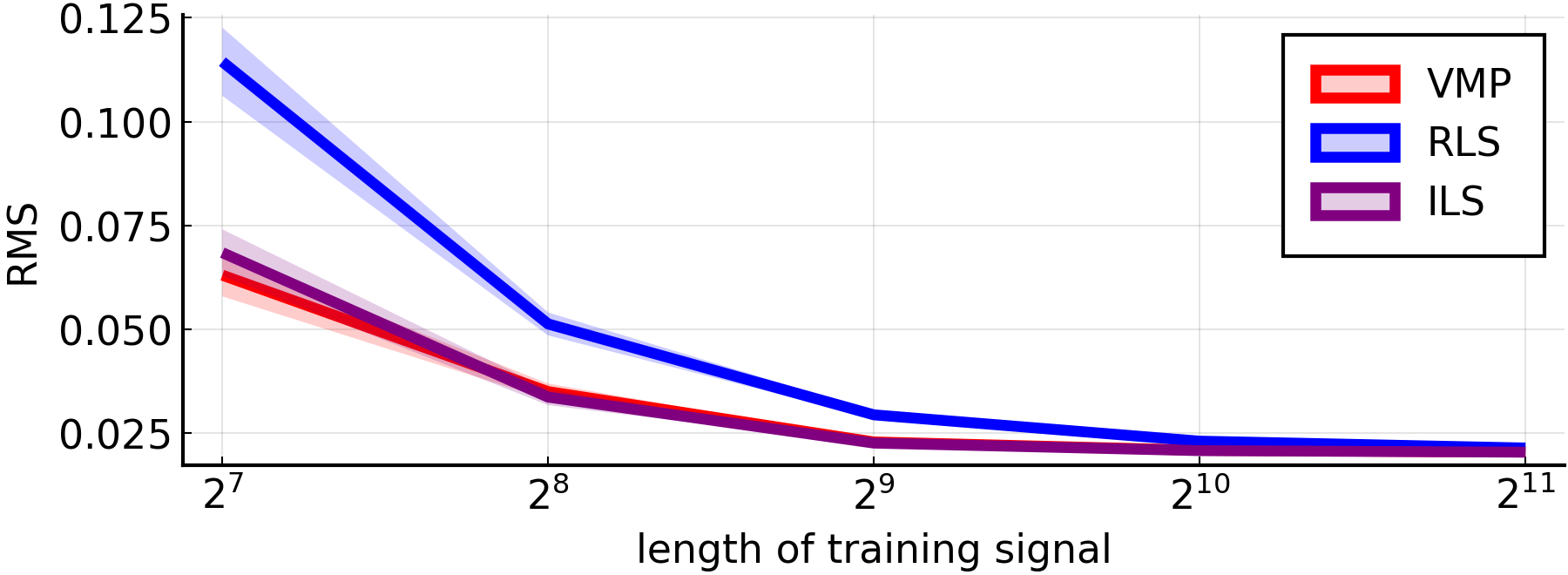
Figure 2: Simulation errors for a noise standard deviation of $0.02$. Average RMS (standard errors as ribbon) by length of training signal.

VI-B Results

Figure 2 shows the simulation errors of the three estimators as a function of the number of training samples. VMP outperforms RLS, especially for small sample sizes. This is due to the inclusion of the prior distributions and the regularizing effect of the parameter posterior on the predictions. VMP performs on par with ILS, which was trained offline. As sample size grows, the three estimators converge to the same level of performance.

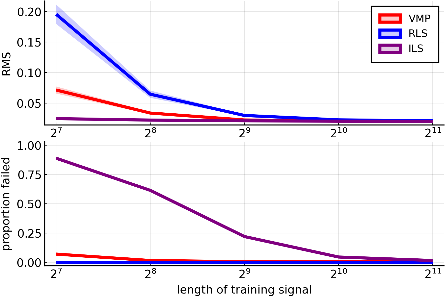
Figure 3: 1-step ahead prediction errors for noise std. dev. $0.2$. (Top) Average RMS (standard errors as ribbons) by length of training signal. (Bottom) Proportion of experiments failed due to diverging parameter estimates.

Figure 3 (top) shows the 1-step ahead prediction errors as a function of the number of training samples. VMP still consistently outperforms RLS, but is no longer on par with ILS. Although ILS performs well, it also tends to diverge in small sample sizes: it would initially produce a prediction with just a slightly larger magnitude, but when the accompanying prediction error was incorporated back into the model, the next prediction would be even larger in magnitude. Figure 3 (bottom) plots the proportion of failed experiments, i.e., those with diverging predictions, for all three estimators as a function of training signal length. ILS diverges less often as training signal length increases, with most of the failures having disappeared after 1024 samples.

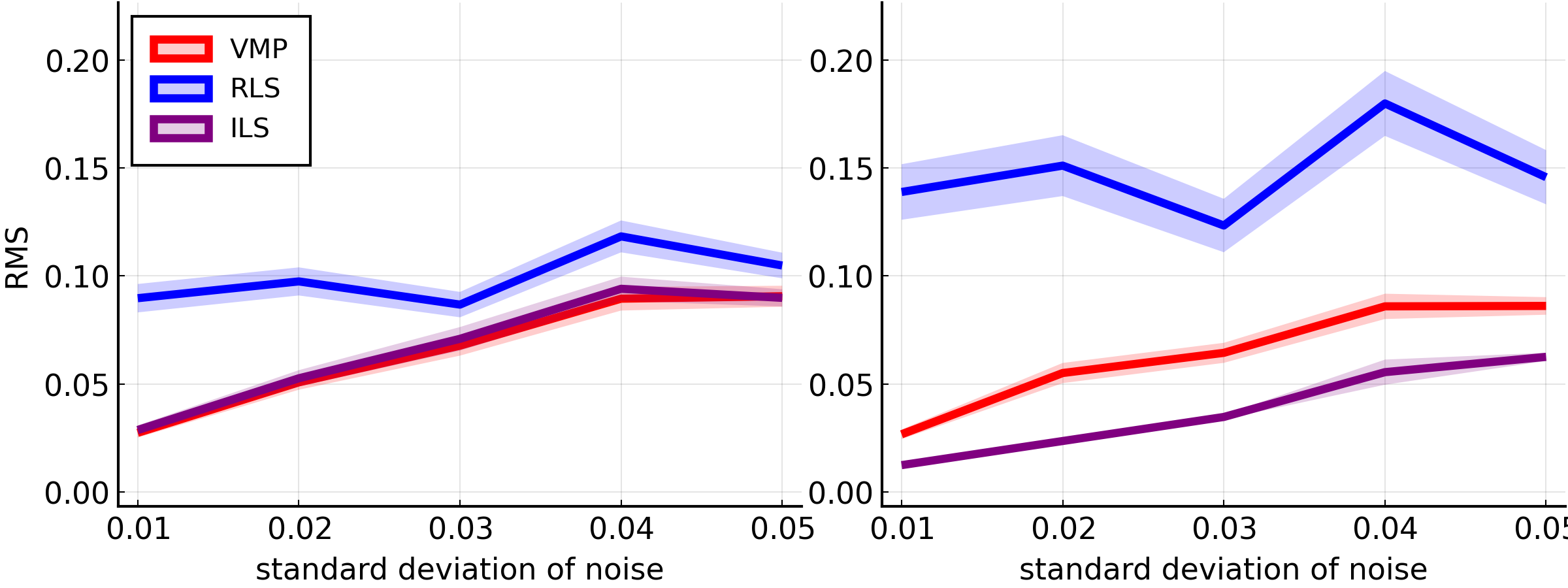
Figure 4: Average RMS (standard errors as ribbons) as a function of system noise, for training signals of length $128$. Simulation (left) and 1-step ahead prediction (right).

In our second experiment, we keep the training signal length fixed at $128$ and vary the standard deviation of the system’s noise. Figure 4 shows the average RMS of the three estimators, along with the standard errors, for simulation (left) and 1-step ahead prediction (right). VMP outperforms RLS for all levels of noise, but especially in the low noise levels. VMP performs on par with ILS during simulation but not during 1-step ahead prediction.

VII Discussion

Variational message passing is a modular procedure and can be automatized: tools such as ForneyLab.jl contain factor nodes in the form of standard parametric distributions, deterministic operations and common filters [23]. The advantage of modularity is that different models can be combined without the need for re-deriving parameter update equations [24]. Among others, this allows for straightforward extensions towards hierarchical models and time-varying parameter estimates [25]. The main limitation of variational message passing is that it requires some form of conditional conjugacy in the prior distributions and recognition factors. Non-conjugate message passing is possible, but often comes at higher computational cost [26].

VIII Conclusion

We proposed a variational message passing algorithm for online system identification in polynomial NARMAX models. We show how to recursively update parameter posterior distributions and how to predict future outputs from given inputs. We demonstrated empirically that our estimator outperforms a recursive least-squares estimator and performs on par with an iterative least-squares estimator trained offline.

IX Acknowledgements

This work was partly financed by research programs ZERO (no. P15-06) and EDL (no. P16-25), funded by the Netherlands Organisation for Scientific Research (NWO).

References

• [1] S. A. Billings, Nonlinear system identification: NARMAX methods in the time, frequency, and spatio-temporal domains.   John Wiley & Sons, 2013.
• [2] K. P. Murphy, Machine learning: a probabilistic perspective.   MIT press, 2012.
• [3] S. Särkkä, Bayesian filtering and smoothing.   Cambridge University Press, 2013.
• [4] V. Peterka, “Bayesian approach to system identification,” in Trends and Progress in System Identification.   Elsevier, 1981, pp. 239–304.
• [5] T. B. Schön, F. Lindsten, J. Dahlin, J. Wågberg, C. A. Naesseth, A. Svensson, and L. Dai, “Sequential Monte Carlo methods for system identification,” IFAC-PapersOnLine, vol. 48, no. 28, pp. 775–786, 2015.
• [6] D. M. Blei, A. Kucukelbir, and J. D. McAuliffe, “Variational inference: A review for statisticians,” Journal of the American Statistical Association, vol. 112, no. 518, pp. 859–877, 2017.
• [7] K. J. Friston, N. Trujillo-Barreto, and J. Daunizeau, “DEM: a variational treatment of dynamic systems,” Neuroimage, vol. 41, no. 3, pp. 849–885, 2008.
• [8] J. Daunizeau, K. J. Friston, and S. J. Kiebel, “Variational Bayesian identification and prediction of stochastic nonlinear dynamic causal models,” Physica D: Nonlinear Phenomena, vol. 238, no. 21, pp. 2089–2118, 2009.
• [9] A. A. Meera and M. Wisse, “Free energy principle based state and input observer design for linear systems with colored noise,” in American Control Conference, 2020, pp. 5052–5058.
• [10] R. S. Risuleo, G. Bottegal, and H. Hjalmarsson, “Variational Bayes identification of acyclic dynamic networks,” IFAC-PapersOnLine, vol. 50, no. 1, pp. 10 556–10 561, 2017.
• [11] J. N. Hendriks, F. K. Gustafsson, A. H. Ribeiro, A. G. Wills, and T. B. Schön, “Deep energy-based NARX models,” IFAC-PapersOnLine, vol. 54, no. 7, pp. 505–510, 2021.
• [12] H.-A. Loeliger, “An introduction to factor graphs,” IEEE Signal Processing Magazine, vol. 21, no. 1, pp. 28–41, 2004.
• [13] S. Korl, “A factor graph approach to signal modelling, system identification and filtering,” Ph.D. dissertation, ETH Zurich, 2005.
• [14] J. Dauwels, “On variational message passing on factor graphs,” in IEEE International Symposium on Information Theory, 2007, pp. 2546–2550.
• [15] K. Fujimoto and Y. Takaki, “On system identification for ARMAX models based on the variational Bayesian method,” in Conference on Decision and Control.   IEEE, 2016, pp. 1217–1222.
• [16] Y. Lu, S. Khatibisepehr, and B. Huang, “A variational Bayesian approach to identification of switched ARX models,” in IEEE Conference on Decision and Control, 2014, pp. 2542–2547.
• [17] W. M. Kouw, “Online system identification in a Duffing oscillator by free energy minimisation,” in International Workshop on Active Inference.   Springer, 2020, pp. 42–51.
• [18] W. R. Jacobs, T. Baldacchino, T. Dodd, and S. R. Anderson, “Sparse Bayesian nonlinear system identification using variational inference,” IEEE Transactions on Automatic Control, vol. 63, no. 12, pp. 4172–4187, 2018.
• [19] J. S. Yedidia, W. T. Freeman, and Y. Weiss, “Constructing free-energy approximations and generalized belief propagation algorithms,” IEEE Transactions on Information Theory, vol. 51, pp. 2282–2312, 2005.
• [20] D. Khandelwal, M. Schoukens, and R. Tóth, “On the simulation of polynomial NARMAX models,” in IEEE Conference on Decision and Control, 2018, pp. 1445–1450.
• [21] M. H. Hayes, Statistical digital signal processing and modeling.   John Wiley & Sons, 2009.
• [22] R. Pintelon and J. Schoukens, System identification: a frequency domain approach.   John Wiley & Sons, 2012.
• [23] M. Cox, T. van de Laar, and B. de Vries, “Forneylab.jl: Fast and flexible automated inference through message passing in julia,” in International Conference on Probabilistic Programming, 2018.
• [24] İ. Şenöz, A. Podusenko, W. M. Kouw, and B. de Vries, “Bayesian joint state and parameter tracking in autoregressive models,” in Conference on Learning for Dynamics and Control, 2020, pp. 1–10.
• [25] A. Podusenko, W. M. Kouw, and B. de Vries, “Message passing-based inference for time-varying autoregressive models,” Entropy, vol. 23, no. 6, p. 683, 2021.
• [26] D. Knowles and T. Minka, “Non-conjugate variational message passing for multinomial and binary regression,” Advances in Neural Information Processing Systems, vol. 24, pp. 1701–1709, 2011.