Perceval: A Software Platform for Discrete Variable Photonic Quantum Computing
Abstract
We introduce Perceval, an open-source software platform for simulating and interfacing with discrete-variable photonic quantum computers, and describe its main features and components. Its Python front-end allows photonic circuits to be composed from basic photonic building blocks like photon sources, beam splitters, phase-shifters and detectors. A variety of computational back-ends are available and optimised for different use-cases. These use state-of-the-art simulation techniques covering both weak simulation, or sampling, and strong simulation. We give examples of Perceval in action by reproducing a variety of photonic experiments and simulating photonic implementations of a range of quantum algorithms, from Grover’s and Shor’s to examples of quantum machine learning. Perceval is intended to be a useful toolkit for experimentalists wishing to easily model, design, simulate, or optimise a discrete-variable photonic experiment, for theoreticians wishing to design algorithms and applications for discrete-variable photonic quantum computing platforms, and for application designers wishing to evaluate algorithms on available state-of-the-art photonic quantum computers.
1 Introduction
Quantum computing has gained huge interest and momentum in recent decades because of its promise to deliver computational advantages and speedups compared to the classical computing paradigm. The essential idea is that information processing takes place on physical devices, and if the components of those devices behave according to the laws of quantum rather than classical physics then it opens the door to exploiting quantum effects to process information in radically different and potentially advantageous ways.
Quantum algorithms like Shor’s factorisation algorithm [1], which gives an exponential speedup over its best known classical counterpart, or Grover’s search algorithm [2], which gives a quadratic speedup over its classical counterparts, are often cited, and have captured the imagination and provided motivation for the rapid developments that have taken place in quantum technologies. However, for such algorithms to have practical significance will require large-scale fault-tolerant quantum computers. Yet the quantum devices that are available commercially or in research laboratories today are somewhat more limited and belong, for now at least, to the so-called noisy-intermediate scale quantum (NISQ) regime [3].
Of course NISQ devices are a necessary step on the path to large-scale fault-tolerant quantum computers, but in principle they could already enable quantum computational advantages [4] – in which they could outperform even the most powerful classical supercomputers available today – for tasks with practical relevance. Several experiments have already claimed to demonstrate quantum computational advantage in sampling tasks [5, 6, 7, 8, 9]. The practical significance of these is still being explored [10, 11, 12], but meanwhile many other promising proposals for quantum algorithms that may deliver practical advantages in this regime are also being pursued. Among others, these include the quantum variational eigensolver [13], universal function approximators like that of [14] (both of which we will return to later in this paper), the quantum approximate optimisation algorithm [15], as well as a host of other algorithms [16] with applications that range from chemistry [17, 18] and many-body physics [19, 20] to combinatorial optimisation [21, 22] and machine learning [23, 24].
In fact, a number of technological routes to building quantum computers are being actively pursued, in which quantum information is encoded in very different kinds of physical systems. These include matter-based approaches that rely on superconducting circuits, cold atoms, or trapped ions, but also light-based approaches in which photons are the basic information-carrying systems. Among these, photons have a privileged status, as they are the natural and indeed only viable support for communicating quantum information, which will eventually be required for networking quantum processors and devices. As such they will necessarily be a part of any longer-term developments in quantum computational hardware and infrastructure. More than this, photons provide viable routes to both NISQ [25] and large-scale fault-tolerant quantum computing through measurement-based models [26, 27] in their own right.
Perceval is a complete and efficient software platform for the discrete variable (DV) model for photonic quantum computing.111Perceval does not aim to treat the continuous variable (CV) model of photonic quantum computing, which is concerned with infinite dimensional observables of the electromagnetic field, and which is the natural realm of the Strawberry Fields platform [29].It especially uses Fock state descriptions of photons generated by sources, evolving through linear optical networks – composed for example of beam splitters, phase shifters, waveplates or other linear optical components – and then being detected. The familiar qubit and measurement-based models for quantum computing can be encoded within the DV model (see e.g. [25, 26]). However, the DV model is also of significant interest in its own right – not least because it has led to some of the first proposals [28] for quantum computational advantage to be demonstrated with NISQ devices. This concerns a computational problem known as Boson Sampling, discussed in detail in Section 4.2, which essentially consists of sampling from the output distribution of photons that interfere in a generic interferometer. We will also demonstrate direct DV photonic approaches to quantum machine learning in Section 4.6.
Perceval’s features can be useful for designing, optimising, simulating, and eventually transpiling DV linear optical circuits and executing them on cloud-based physical processors. Although Perceval provides bridges (see Section 3.2.6) with other open-source quantum computing toolkits [30] such as Qiskit [31], it further allows users to work at a level that is closer to the photonic hardware than these toolkits regular gate-based qubit quantum circuit model, which is already the focus of a number of other software platforms. It is also more flexible and supports many more functionalities than existing packages for linear optical quantum systems [32]. The finer-grained control of the physical hardware can be valuable both for the NISQ regime, where it is crucial to achieve the maximum performance from the specific hardware resources available, and for optimising the building block photonic modules in schemes for reaching the large-scale fault-tolerant regime.
Perceval is intended to be useful for experimentalists wishing to design photonic experiments, including allowing for realistic modelling of noise and imperfections, and for computer scientists and theoreticians seeking to develop algorithms and applications for photonic quantum computers. It is an open source platform that is intended for community development via GitHub, the project forum website and an updated documentation.
Perceval integrates several state-of-the-art algorithms for running simulations optimised with low-level single instruction, multiple data (SIMD) implementations, allowing users to push close to the limits of classical simulability with desktop computers. Extensions to the framework are also intended for high-performance computing (HPC) cluster deployment which can permit simulation to scale further. Since version 0.7, Perceval is able to run samples from real photonic chips through the Cloud, giving the user access in real-time to the exact hardware characteristics of the photonic source (brightness, purity, indistinguishability), the chip, and the detectors. Remote computers are also available if the user wants to perform classical simulation with greater computational power.222More details on https://perceval.quandela.net/docs/notebooks/Remote%20computing.html
The remainder of this white paper is structured as follows. We provide some brief background on photonic quantum computing in Section 2, before outlining the structure and key features of Perceval in Section 3, and then go on to give a number of illustrative examples of Perceval in action in Section 4. The code of the examples can be found in Appendix B. This paper is based on version 0.7.3 of Perceval.
2 Photonic Quantum Computing
Similar to the qubit quantum circuit model, the DV photonic model can be presented as a gate-based model, in which states are prepared, transformed as they are acted upon by gates, and measured.
We consider a number of spatial modes. Physically these could correspond to waveguides in an integrated circuit, optical fibres, or paths in free space. Photon sources prepare initial states in these spatial modes. These are number states , where is the number of photons in the mode, or superpositions of number states. We use the shorthand notation for a two-mode system with state in the first and in the second, etc. Unless otherwise specified, photons are assumed to be indistinguishable. Sometimes we will wish to keep track of the polarisation of the photons, which can be achieved by further splitting each spatial mode into two polarisation modes, e.g. horizontal (denoted by ) and vertical (denoted by ), and recording the (superpositions of) number states for each. Perceval also allows the possibility of tracking other attributes of photons.
Transformations are performed on the states by evolving them through linear optical networks. The simplest linear optical operations (gates) are: phase shifters, which act on a single spatial mode, and beam splitters, which act on pairs of spatial modes. These operations preserve photon number and are best described as unitary matrices that act on the creation operator of each mode (see [33, 34] for a more detailed treatment). A creation operator is defined by its action . The unitary associated with a phase shifter with phase parameter is simply the scalar , while in the Rx convention the unitary matrix associated to a beam splitter is given in Equation 1. We have included for clarity the basis on which the matrix acts in gray above and on the left.
| (1) |
where the parameter relates to the reflectivity and denotes the state in which the photon travels in the first spatial mode. Perceval introduces all theoretically equivalent beam splitter matrix conventions as shown in Table 1. The action of any linear optical circuit is thus given by the unitary matrix obtained by composing and multiplying the matrices associated with its elementary components. Interestingly, it can be shown that conversely any unitary evolution can be decomposed into a combination of beam splitters and phase shifters, e.g. in a ‘triangular’ [35] or ‘square’ [36] array.
Perceval also allows for swaps or permutations of spatial modes, and can include operations like waveplates, which act on polarisation modes of a single spatial mode and are described by the following unitary [37]:
| (2) |
Here is a parameter proportional to the thickness of the waveplate and represents the angle of the waveplate’s optical axis in the plane. Especially important is the case that , known as a half-wave plate, which rotates linear polarisations in the plane. Quarter-wave plates () convert circular polarisations to linear ones (e.g. ) and vice-versa.
Polarising beam splitters will convert a superposition of polarisation modes in a single spatial mode to the corresponding equal-polarisation superposition of two spatial modes, and vice versa, and so in this sense allow us to translate between polarisation and spatial modes. The unitary matrix associated to a polarising beam splitter acting on the tensor product of the spatial mode and the polarisation mode is
| (3) |
where denotes the single-photon state in which the photon travels in the first spatial mode with a horizontal polarisation.
Similarly then, any unitary evolution on spatial and polarisation modes can be decomposed into an array of polarising beam splitters, beam splitters and phase shifters.
Finally measurement, or readout, is made by single photon detectors (these may be partially or fully number resolving). Both photon generation and measurement are non-linear operations. In particular, measurements can be used to induce probabilistic or post-selected non-linearities in linear optical circuits. This could be used to further implement feedforward, whereby measurement events condition parameters further along in a circuit.
The basic post-selection-, feedforward- and polarisation-free (without polarisation modes or operations) fragment of the DV model described above is precisely the model considered by Aaronson and Arkhipov in [28]. For classical computers, simulating this simple model, straightforward though its description may be, is known to be -hard, and up to complexity-theoretic assumptions the same is true for approximate classical simulation. The reason for this essentially comes down to the fact that calculating the detection statistics requires evaluating the permanents of unitary matrices, a problem which itself is known to be P-hard [38]. We describe this in a little more detail when we look at Boson Sampling in Section 4.2.
Similarly the polarisation-free fragment was shown by Knill, Laflamme and Milburn to be quantum computationally universal [25]. In particular, it can be used to represent qubits and qubit logic gates.
Just as the bit – any classical two level system – is generally taken as the basic informational unit in classical computer science, the qubit – any two level quantum system – is usually taken as the basic informational unit in quantum computer science. Photons have many degrees of freedom and offer a rich variety of ways to encode qubits. One of the most common approaches is to use the dual-rail path encoding of [25]. Each qubit is encoded by one photon which may be in superposition over two spatial modes, which correspond to the qubit’s computational basis states:
| (4) |
Single-qubit unitary gates are particularly straightforward to implement in this encoding, requiring only a fully parametrisable beam splitter, as in Equation 1, and a phase shifter. An example of an entangling two-qubit gate (), which uses heralding, i.e. post-selection over auxiliary modes, will be presented in Section 3.
Another common qubit encoding is the polarisation encoding, and indeed versions of the KLM scheme also exist for this encoding [39]. Here each qubit is encoded in the polarisation degree of freedom of a single photon. This encoding will be used in the example of Section 4.3. In practice, encodings may be chosen based on the availability or ease of implementation of different linear optical elements in laboratory settings. For instance path-encoding is at present more accessible than polarisation encoding in integrated optics, where linear optical circuits are implemented ‘on-chip’. Although we have discussed ways of encoding qubit quantum circuits into the DV model, it should be reiterated that the DV model has interesting features in its own right, and the examples of Boson Sampling in Section 4.2 and quantum machine learning in Section 4.6 give some illustrations of interesting applications that bypass qubit descriptions.
We have presented the idealised DV model, but it is important to note that in realistic implementations various noise, imperfections, and errors will arise. Perceval is also intended as a tool for designing, modelling, simulating and optimising realistic DV linear optical circuits and experiments, and to incorporate realistic noise-models. We briefly demonstrate how Perceval handles imperfect photon purity at source and distinguishability due to imperfect synchronisation in Section 4.1. Other relevant factors are losses at all stages from source to detection, imperfect or imperfectly characterised linear optical components, cross-talk effects, detector dark-counts, etc. Future versions of Perceval will contain increasingly sophisticated and parametrised modelling of such factors.
3 Presentation of Perceval
3.1 Global Architecture
Perceval is a linear optical circuit development framework whose design is based on the following core ideas:
-
•
It is simple to use, both for theoretical and experimental physicists and for computer scientists.
-
•
It does not constrain the user to any framework-specific conventions that are theoretically equivalent (for example it was noticed early on that many different conventions for beam splitters can be found in the literature).
-
•
It provides state-of-the-art optimised algorithms – as benchmarked on specific use cases.
-
•
It provides – when possible and appropriate – access to symbolic calculations for finding analytical solutions.
-
•
It provides companion tools, such as a unitary matrix toolkit, and LaTeXor HTML rendering of algorithms.
-
•
It incorporates realistic, parameterisable error and noise modelling.
-
•
It aims to provide a seamless transition from simulators to actual photonic processors (QPU). As such, most of the programmatic interfaces are designed for QPU control. In particular, fixing a specific QPU automatically hides methods giving access to properties (such as probability amplitudes) and features which would be unavailable on the actual hardware.
Perceval is a modular object-oriented Python code, with optimised functions written in C making use of SIMD vectorisation. In the following section, we give an overview of the main classes available to the user. A full documentation is maintained on GitHub and available online through the project website.
3.2 Main Classes
3.2.1 States
Information in a linear optical circuit is encoded in the state of photons in certain “modes” that are defined by the circuit designer. States are implemented in Perceval by the following two classes:
-
•
BasicState is used to describe Fock states of photons over modes.By default, photons are indistinguishable but each photon can be annotated, controlling its distinguishability. An annotation is a way to associate additional information to each photon and can thus represent additional degrees of freedom — for instance, polarisation is represented as a photon annotation;
-
•
StateVector extends BasicState to represent superpositions of states.
3.2.2 Circuits
The Circuit class provides a practical way to assemble a linear optical circuit from predefined elementary components, other circuits, or unitary matrices. It can also compute the unitary matrix associated to a given circuit, or conversely decompose a unitary into a linear optical circuit consisting of user-defined components. A library of predefined elementary components is provided (see Table 1). Those components can be added on the desired mode(s) on the right of a Circuit with the \pythCircuit.add(modes, component) method. An example of code using this class can be found in Code 1.
Name
Unitary Matrix
Representation
Beam Splitter
convention:
convention:
convention:
![[Uncaptioned image]](/html/2204.00602/assets/images/BSRx.png)
![[Uncaptioned image]](/html/2204.00602/assets/images/BSRy.png)
![[Uncaptioned image]](/html/2204.00602/assets/images/BSH.png) Phase Shifter
Phase Shifter
![[Uncaptioned image]](/html/2204.00602/assets/images/ps.png) Mode Permutation
Mode Permutation
![[Uncaptioned image]](/html/2204.00602/assets/images/perm.png) Wave Plate
Wave Plate
![[Uncaptioned image]](/html/2204.00602/assets/images/wp.png) Polarising
Beam Splitter
Polarising
Beam Splitter
![[Uncaptioned image]](/html/2204.00602/assets/images/pbs.png) Polarising Rotator
Polarising Rotator
![[Uncaptioned image]](/html/2204.00602/assets/images/pr.png) Time Delay
Time Delay
![[Uncaptioned image]](/html/2204.00602/assets/images/dt.png)
3.2.3 Back-ends
Perceval allows the user to choose between its four back-ends – CliffordClifford2017, Naive, SLOS and Stepper – each one taking a different computational approach to circuit simulation. They perform the following tasks:
-
•
Sample individual single output states – CliffordClifford2017;
-
•
Compute the probability, or probability amplitude, of obtaining a given output state from a given input state – Naive;
-
•
Describe the exact complete output state – SLOS, Stepper.
The CliffordClifford2017 Back-end.
This back-end is the implementation of the algorithm introduced in [40]. The algorithm, applied to Boson Sampling, aims to “produce provably correct random samples from a particular quantum mechanical distribution”. Its time and space complexity are respectively and . The algorithm has been implemented in C++, and uses an adapted Glynn algorithm [41] to efficiently compute simultaneous “sub-permanents”.
Recently, the same authors have proposed a faster algorithm in [42] with an average time complexity of for a number of modes which is linear in the number of photons , where:
| (5) |
The Naive Back-end.
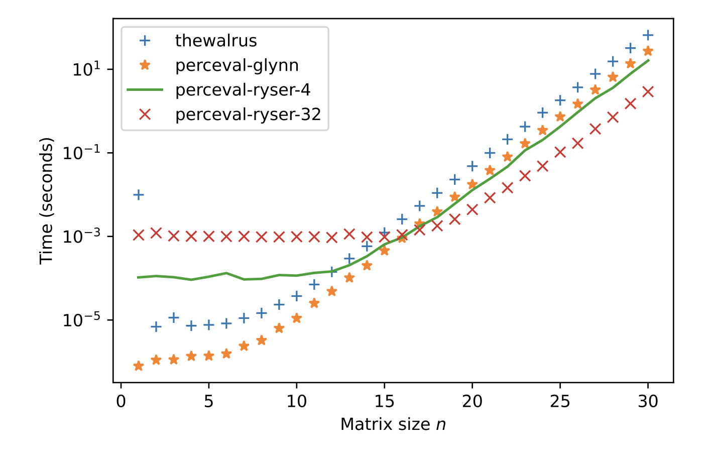
This back-end implements direct permanent calculation and is therefore suited for single output probability computation with small memory cost. Both Ryser’s [43] and Glynn’s [41] algorithms have been implemented. Extra care has been taken on the implementation of these algorithms, with usage of different optimisation techniques including native multithreading and SIMD vectorisation primitives. A benchmark of these algorithms against the implementation present in the The Walrus library [44] is provided in Figure 4.
The SLOS Back-end.
The Strong Linear Optical Simulation SLOS algorithm developed by a subset of the present authors is introduced in [45]. It unfolds the full computation path in memory, leading to a remarkable time complexity of for computing the full distribution. The current implementation also allows restrictive sets of outputs, with average computing time in for single output computation. As discussed in [45], it is possible to use the SLOS algorithm in a hybrid manner that can combine both weak and strong simulation, though it has not yet been implemented in the current version of Perceval. The tradeoff in the SLOS algorithm is a huge memory usage of that limits usage to circuits with photons on personal computers and with photons on super-computers.
The Stepper Back-end.
This back-end takes a completely different approach. Without computing the circuit’s overall unitary matrix first, it applies the unitary matrix associated with the components (see Table 1) in each layer of the circuit one-by-one, simulating the evolution of the state vector. The complexity of this back-end is therefore proportional to the number of components. It has the nice features that:
-
•
it can support more complex components like Time Delay;
-
•
it is very flexible with simulating noise in the circuit, like photon loss, or more generally with simulating any non-linear operation the user would wish to implement;
-
•
it simplifies the debugging of circuits by exposing intermediate states.
The Stepper back-end is really meant for circuit simulation with losses or non linear components. In all other cases, it is more efficient to directly consider the unitary matrix of the whole circuit and compute the output state with SLOS, instead of performing a computation for each component using the Stepper back-end.
Theoretical performances and specific features of the different back-ends are summarised in Table 2.
Feature CC2017 SLOS Naive Stepper Sampling Efficiency (**) Single Output Efficiency N/A (**) Full Distribution Efficiency N/A Probability Amplitude No Yes Yes Yes Supports Symbolic Computation No No Yes Yes Supports Time-Circuit No No No Yes Practical Limits (***)
3.2.4 Processors
The Processor class allows the user to emulate a real photonic quantum processor, taking into account the single photon source, the circuit and the detectors. The Perceval source model allows tuning of the transmittance, multiple photon emission probability, and indistinguishability. By default, the source is perfect. The circuit can be composed of unitary or non-unitary components. Detector imperfections can be emulated – one can switch between number resolving detectors and threshold detectors. Post-selection features can also be added to a Processor via heralded modes and/or a final post-selection function. See the Appendix A.4 for more details.
3.2.5 Algorithms
3.2.6 Bridges to Other Quantum Computing Toolkits
In order to facilitate work across multiple platforms, Perceval provides both a catalog of predefined components and specific converters:
-
•
The predefined component catalog is available in Perceval.components.catalog, where each element is an instance of CatalogItem providing a ready-to-use circuit (as_circuit() method), a processor (as_processor() method), and a complete documentation (doc property).
-
•
Converters to Perceval from other frameworks are available in perceval.converters. Their task is to provide a photonic Perceval equivalent of circuits and algorithms defined in other open source frameworks. Currently a qiskit555https://qiskit.org converter is available and converters for tket and QLM are in development.
Examples for both tools are provided in a notebook of the Perceval documentation.
3.2.7 Step-by-Step Example
The following code implements a simple linear optical circuit corresponding to a path-encoded gate (after post-selection in the coincidence basis) [46].
Let us explain how it works. We remind that the gate is a two-qubit gate that acts in the following way:
| (6) |
i.e. it’s a controlled-not gate where the first qubit acts as control and the second qubit is the target. We use dual-rail encoding (see Equation 4) and thus need four spatial modes to represent the target and the control. We additionally need two auxiliary empty modes to implement this post-selected linear optical . The circuit is made of three central beam splitters of reflectivity , whereas the two to the left and right of the central ones have a reflectivity of . The corresponding circuit displayed by Perceval is depicted in Figure 2.
The first and last spatial modes correspond to the auxiliary empty modes, the second and third to the control qubit, and the fourth and fifth to the target qubit. The associated unitary matrix acting on the six spatial modes computed with Perceval is displayed in Figure 3.
We then need to post-select on measuring two (dual-rail encoded) qubits in the modes corresponding to the target and the control, i.e. on measuring exactly one photon in the second or third spatial modes and exactly one photon in the fourth or fifth spatial modes. One can check that this measurement event happens with probability – we call this number the ‘performance’ of a post-selected gate. We say that the error rate is if the implementation of the gate is perfect (after post-selection). This computation can be done with Perceval: we define a processor, use the SLOS back-end, and perform a full output distribution and performance analysis, as illustrated in Figure 4.
| 00 | 01 | 10 | 11 | |
| 00 | 1 | 0 | 0 | 0 |
| 01 | 0 | 1 | 0 | 0 |
| 10 | 0 | 0 | 0 | 1 |
| 11 | 0 | 0 | 1 | 0 |
=> performance=1/9, fidelity=100.0%
4 Perceval in Action
In this section we provide examples of the Perceval software in use. We reproduce several photonic experiments that implement important quantum algorithms and then demonstrate a photonic quantum machine learning algorithm on a simulated photonic quantum processor.
4.1 The Hong-Ou-Mandel Effect
4.1.1 Introduction
The Hong-Ou-Mandel (HOM) effect [47] is an interference effect between pairs of indistinguishable photons, which, when incident on a balanced beam splitter via the respective input modes, will bunch and emerge together in either of the output modes with equal probability. In 2002, Santori et al. demonstrated the HOM effect with a unique source of single photons [48], evidencing the indistinguishability of consecutive photons and paving the way to many developments in experimental quantum optics.
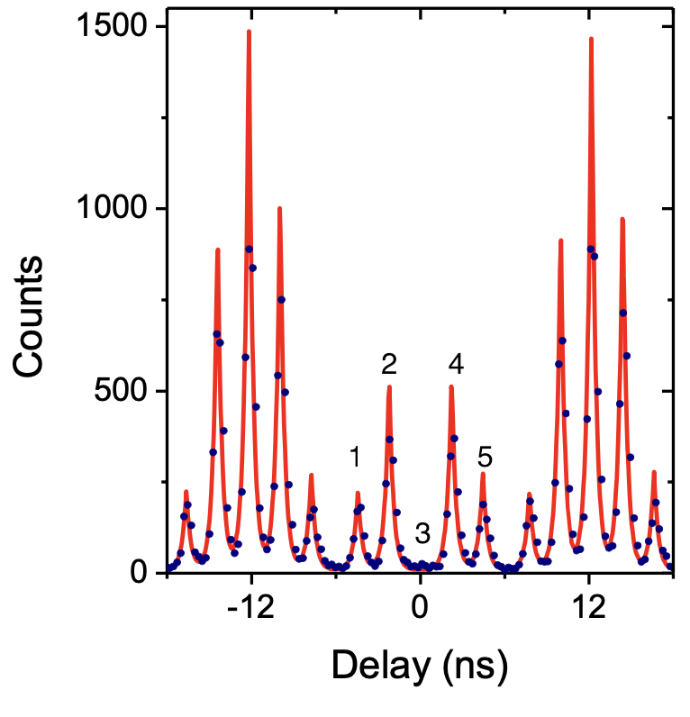
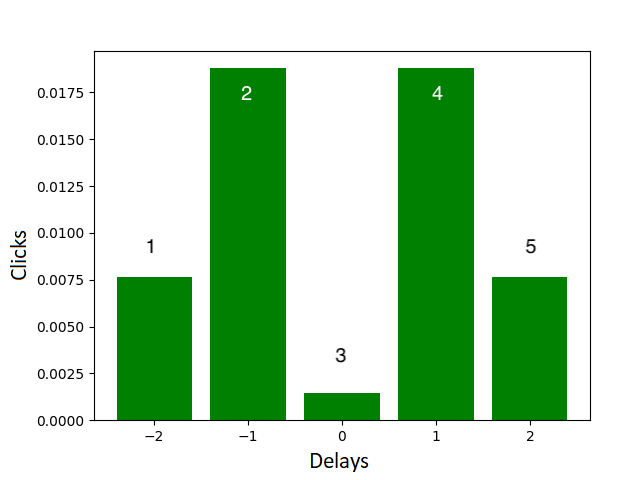
In this experiment, “two pulses separated by ns and containing or photons, arrive through a single-mode fibre. The pulses are interfered with each other using a Michelson-type interferometer with a ( ns) path-length difference. […] The interferometer outputs are collected by photon counters, and the resulting electronic signals are correlated using a time-to-amplitude converter followed by a multi-channel analyser card, which generates a histogram of the relative delay time between a photon detection at one counter () and the other ()” [48]. An equivalent experiment was carried out in [49] with similar results, presented in Figure 5.
4.1.2 Perceval Implementation
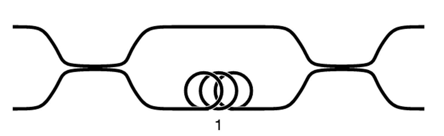
The implementation on Perceval uses a simple circuit composed of a beam splitter (corresponding to the main beam splitter of [48, Figure 3(a)]), the lower output mode of which then passes through a -period time-delay, and then a second beam splitter on the modes where the interference happens.
The circuit and result are presented in Figure 6. The resolution is less fine-grained than the original experiments due to the absence of modelling of photon length in the current implementation of Perceval. However, we clearly recognise the same distinctive peaks in the relative amplitude. The very small coincidence rate at is the signature of photon interference. The implementation of the algorithm is provided in Appendix.
4.2 Boson Sampling
4.2.1 Introduction
Boson Sampling666The technical introduction to the problem here draws heavily on a previous work by a subset of the authors of this paper [50]. is a sampling problem originally proposed by Aaronson and Arkhipov [28]. We give a detailed description of the problem below. It essentially consists of sampling from the probability distribution of outcome detection coincidences when single photons are introduced into a random linear optical circuit.
Let be positive integers with . Let be the set of all possible tuples of non-negative integers , with . Let be an Haar-random unitary matrix. From we construct an matrix as follows. For a given , first construct an matrix by copying times the th row of . Then, for a given (fixed) , construct from by taking copies of the th column of . Let be the permanent [51, Chapter 7] of , and let
| (7) |
It can be shown that , and that the set is a probability distribution over outcomes [28].
Let be a given precision. Approximate Boson Sampling can then be defined as the problem of sampling outcomes from a probability distribution such that
| (8) |
where denotes the total variational distance between two probability distributions. Exact Boson Sampling corresponds to the case in which .
For , it was shown in [28] that:
-
•
No classical algorithm can solve Exact Boson Sampling in time ,
-
•
No classical algorithm can solve Approximate Boson Sampling in time , unless some widely accepted complexity theoretic conjectures turn out to be false.
These hardness results are closely related to the hardness of computing the permanent of matrices [38, 28].
On the other hand, Boson Sampling can be solved efficiently in the exact case on a photonic quantum device which is noiseless [28], while the approximate version only requires sufficiently low noise levels [52, 53, 54]. This is done by passing identical single photons through a lossless -mode universal linear optical circuit [35, 36] configured in such a way that it implements the desired Haar-random unitary transformation . Universal here is meant in the sense of photonic unitaries and refers to the ability of the circuit to generate any arbitrary unitary evolution on the creation operators of the modes. A universal linear optical circuit can be configured to implement any unitary chosen from the Haar measure, for example using the recipe of [55]. The input configuration of single photons corresponds to a tuple . We then measure the output modes of the circuit using perfect single photon detectors, and will obtain the output configuration tuple according to the distribution [28]. The detectors should be photon-number resolving in general, but not necessarily when working in the no-collision regime () [28].
4.2.2 Perceval Implementation77footnotemark: 7
88footnotetext: This implementation is accompanied by a notebook.Boson Sampling with single photons in a mode linear optical circuit with up to -photon coincidences at the outputs was reported in [56]. In this Section, we report the results of a noiseless Boson Sampling simulation performed with Perceval for single photons and modes. For this Boson Sampling, the total number of possible output states is [28].
For an input state of photons in arbitrarily chosen modes , we generated Haar random unitaries, and performed for each of these unitaries runs of Boson Sampling, where each run consists of sampling a single output. In total, we collected samples.
The classical algorithm for Boson Sampling integrated into Perceval and which was used for this simulation is that of Clifford and Clifford [40]. Note that faster versions of this algorithm have been found by the same authors in the case where is proportional to [42]. Integration of the algorithm of [42] into Perceval is a subject of on-going work. The simulations were performed on a 32-core 3.1GHz Intel Haswell processor, at the rate of 8547 runs (samples) per second. It took roughly days to collect samples.
Brute-force certification that our simulation has correctly implemented Boson Sampling would require, for each of the 300 Haar random unitaries, calculation of approximately permanents (to get the ideal probability distribution of the Boson Sampler), then performing runs of Boson Sampling using our simulation, in order to get the distribution of the simulated Boson Sampler to within the desired accuracy. Clearly, this task is computationally intractable. In order to get around this issue, while still having some level of confidence that our Boson Sampling simulation has indeed been implemented correctly, we have appealed to computing partial certificates [50, 57]. These certificates are usually efficiently computable, but nevertheless can be used to rule out some common adversarial strategies designed to spoof Boson Sampling [58, 59], although they cannot provably rule out every possible adversarial spoofing strategy [58, 57, 59, 50].
The partial certificate we used here is the probability that all input photons are measured in the first output modes of the Boson Sampler [57], where . We believe this choice of partial certificate is natural for benchmarking our simulation mainly for the following reasons. First, it can be computed straightforwardly from the output probabilities of Boson Sampling. Second, it relies on computing high order marginals, which are most likely difficult to compute efficiently classically [28]. Finally, for some values of , and , can be computed to very good accuracy by using only a polynomial number of samples from the device [57].
| (9) |
where, for a given unitary , is computed as in Equation 7. The average of over the Haar measure of unitaries has been computed analytically in [57]:
| (10) |
We computed an estimate of by computing an estimate of using samples for each of the 300 Haar random unitaries, then performing a uniform average over all these 300 unitaries. Our calculations for various values of , together with the standard deviation of the distribution of are presented in Table 3.
| Std. Dev. |
We observe a good agreement between the analytical values and the values computed with Perceval, in particular when the value of is close to 60. This is to be expected, since these values of are closest to the regime in which , where it has been shown [57] that is polynomially close to one in and , and therefore a number of samples from the Boson Sampler is enough to compute to good precision so as to allow a reliable certification.
As a final remark, note that Perceval can also simulate imperfect Boson Sampling, where the imperfections integrated so far include photon loss and the possibility of multi-photon emissions. For further details we refer the reader to the documentation.
4.3 Grover’s Algorithm
4.3.1 Introduction
Grover’s algorithm [2] is an -runtime quantum algorithm for searching an unstructured database of size . It is remarkable for providing a polynomial speedup over the best known classical algorithm for this task, which runs in time . We now provide an intuitive explanation of how this algorithm works, similar to that which can be found in the Qiskit documentation or in [60].
We work in the -qubit Hilbert space , which allows us to treat a database of size . In its standard formulation, the goal of Grover’s algorithm is to look for an unknown computational basis state , which we will call the target state, with .
Let be the (normalised) uniform superposition of all the computational basis states other than , which is orthogonal to . The uniform superposition of all computational basis states can then be written as
| (11) |
Describing the problem setting in this way allows us to describe Grover’s algorithm in a geometric picture. Indeed, we can now think of the states , , and as lying in a 2-dimensional plane with a basis . For example, forms an angle with respect to (or with respect to ).
Grover’s algorithm relies on the application of two unitaries noted and . The former is an oracle unitary999An oracle is a unitary which the algorithm can apply without having knowledge about its internal implementation. defined on computational basis states as
| (12) |
while the latter is the diffusion unitary is defined as
| (13) |
where the -qubit identity matrix. On the uniform superposition, the unitary acts as
| (14) |
Geometrically, reflects the state through the vector . Let’s call the resulting reflected state . Then, performs a reflection of through the vector . Let the resulting reflected state be denoted . One can see that these transformations keep the states in the same 2D-plane, and that forms an angle of with respect to (or with respect to ). The state after applying is thus closer to than the initial state was.
The reflections that we described correspond to one iteration of Grover’s algorithm. The full algorithm first creates the state by applying Hadamard gates to an input state . It then transforms the state into by applying times the unitary to . Following the geometric reasoning above, the required number of iterations is given by:
| (15) |
where is the ceiling function.
As a closing remark, let us mention that the original version of Grover’s algorithm presented here is non-deterministic, albeit with a probability of success approaching one exponentially quickly with increasing [2]. Fully deterministic versions of Grover’s algorithm can be obtained, for example by using different oracles and diffusion unitaries than those used here [61], or by using two different types of diffusion unitaries while keeping the same [60].
4.3.2 Perceval Implementation1010footnotemark: 10
1111footnotetext: This implementation is accompanied by a notebook.Here we reproduce the photonic demonstration of Grover’s algorithm of [62]. It uses the spatial and polarisation degrees of freedom to implement a mode realisation of the algorithm with two spatial modes. We spell out the correspondence between the marked database element and the associated quantum state in Table 4.
| Marked database element | Quantum state |
Quantum Circuit.
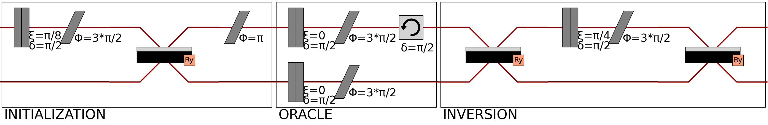
Figure 7 represents the quantum circuit that implements Grover’s algorithm on two qubits, encoded over two spatial modes and their polarisation modes as described in Table 4. It features a state initialisation stage creating a uniform quantum superposition over all states, an oracle stage, and a diffusion stage. Replacing in Equation 15 gives Thus, one application of the oracle and diffusion gates suffices.
Linear Optical Circuit.
The linear optical circuit we will use in our simulation is shown in Figure 8. This circuit was experimentally realised by Kwiat et al. [62] using bulk (i.e. free-space) optics and compiled to limit the number of optical elements introduced in the experimental setup, by moving and combining operations like phase shifts.
Simulation.
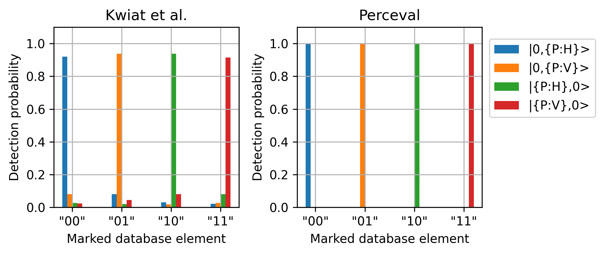
Here, we simulate in Perceval the linear optical circuit of [62] (see Figure 8), a photonic realisation of the quantum circuit in Figure 7, which implements Grover’s algorithm for marked elements , , and 11. The results are displayed in Figure 9, along with the experimental results of Kwiat et al. [62].
4.4 Shor’s Algorithm
4.4.1 Introduction
The problem of factoring an integer is thought to be in -intermediate and the best known classical algorithms only achieve sub-exponential running times. Its classical complexity is well studied since it has been used as the basis of the most widely adopted encryption scheme, Rivest-Shamir-Adleman (RSA) [63], where the secret key consists in two large primes and , while their product is the corresponding public key. In this context, Shor’s algorithm [1] greatly boosted interest in quantum algorithms by showing that such composite numbers can in fact be factored in polynomial time on a quantum computer.
From Period-Finding to Factoring (Classically).
We start by assuming that there exists a period-finding algorithm for functions over integers given as a black-box. This algorithm is used to find the order of integers in the ring , i.e. the smallest value such that . In particular, the values of are sampled at random until the associated is even.
Once such an has been found,121212Values of that verify this property are common in . we have that is a multiple of but not (otherwise the period would be ). We test whether is a multiple of and if so restart the procedure.131313It can be proven that the probability of not restarting at this step is high, and on average the algorithm needs to be repeated only once. Otherwise, we have found a multiple of one of the prime factors since divides a multiple of . Taking the greatest common divisor (GCD) of and easily yields this prime factor. Indeed, the GCD can be found efficiently classically for example by using Euclid’s algorithm.
In summary, all the steps described are basic arithmetic operations, simple to implement on a classical machine, and most of the complexity is hidden in the period-finding algorithm.
Shor’s Quantum Period-Finding Algorithm.
The key contribution of Shor’s work was to show that the period-finding algorithm can be done in polynomial time on a quantum computer.
Indeed, finding the order for a value can be reduced to a problem of phase estimation for the unitary implementing the Modular Exponentiation Function (MEF) on computational basis states. It can be shown that all eigenvalues of these operators are of the form for an integer and the value of interest . The phase estimation algorithm uses as basis the Quantum Fourier Transform and its inverse, along with controlled versions of unitaries of the type up to .141414Using this family of unitaries reduces the precision required of the phase estimation procedure from to constant. This part of the circuit is specific to the value of and and can therefore be optimised once they have been chosen. Although the most costly part of the algorithm in terms of gates, the unitaries - (controlled gates) can still be implemented in polynomial time on a quantum computer, making the overall procedure efficient as well.
4.4.2 Perceval Implementation1515footnotemark: 15
1616footnotetext: This implementation is accompanied by a notebook.Here we reproduce the photonic realisation of Shor’s algorithm from [64].
Quantum Circuit.
The quantum circuit shown in Figure 10 for factoring using parameter , whose order is . It acts on 5 qubits labelled (for the top three) and (for the bottom two). The gates apply a version of the MEF which has been optimised for this specific value of to the qubits in superposition, storing the outcome in qubits . The outcome is given by measuring the qubits , followed by classical post-processing.
Linear Optical Circuit.
Since qubit remains unentangled from the other qubits it can be removed from the optical implementation of this circuit. Furthermore, the gates on can be realised as
| (16) |
where the indices denote the qubits to which the gate is applied (in the case of , the first qubit is the control). Finally, the inverse Quantum Fourier Transform can be performed via classical post-processing, and so does not need to be implemented as a quantum gate in the circuit. The circuit after these simplifications is given in Figure 11.
The expected output state of the circuit above is
| (17) |
We work with path encoded qubits, as in [64]. With path encoding, each gate in the quantum circuit is implemented with a beam splitter with reflectivity between the two paths corresponding to the qubit. In our implementation in Perceval, phase shifters are added to properly tune the phase between each path.
gates are implemented with beam splitters with reflectivity acting on modes: one inner beam splitter creates interference between the two qubits, and two outer beam splitter balance detection probability using auxiliary modes. This optical implementation succesfully yields the output state produced by a gate with probability ; otherwise it creates a dummy state, which can be removed by post-selection.
The circuit implemented in Perceval is illustrated in Figure 12.
The matrix associated to the optical circuit, giving the probability amplitude of each combination of input and output modes, is given in Figure 13.
Simulation.
After entering the initial Fock state associated to the input qubit state we plot the probability amplitudes of the output state, post-selected on Fock states corresponding to a qubit state with path encoding. The results are given in Figure 14.
Output state amplitude: (post-selected on qubit states, not renormalized)
|>
|0,0,0,0> 0j
|0,0,0,1> (0.055555555555555566+0j)
|0,0,1,0> 0j
|0,0,1,1> 0j
|0,1,0,0> (-0.055555555555555557-1.734723475976807e-18j)
|0,1,0,1> (-1.3877787807814457e-17-1.734723475976807e-18j)
|0,1,1,0> (-1.734723475976807e-18j+0j)
|0,1,1,1> 0j
|1,0,0,0> 0j
|1,0,0,1> (-1.3877787807814457e-17+0j)
|1,0,1,0> (-1.734723475976807e-18j+0j)
|1,0,1,1> (-0.055555555555555557-1.734723475976807e-18j)
|1,1,0,0> (1.3877787807814457e-17+0j)
|1,1,0,1> 0j
|1,1,1,0> (0.05555555555555558+0j)
|1,1,1,1> (1.3877787807814457e-17+5.204170427930421e-18j)
After re-normalisation we find that the output amplitudes computed with Perceval match the expected output state described in Equation 17 up to numerical precision.
When decomposing the expected output state in the qubit basis, the qubit states with non-zero amplitude are , , and for qubits . We plot the output distribution of the circuit, post-selected on these states, without re-normalisation; the result is presented in Table 5.
The distribution obtained with Perceval is uniform over each outcome, which matches the expected distribution in [64].
Outcome Distribution Interpretation.
For each outcome, the values of qubits (with ) represent a binary number between 0 and 7, here corresponding to in the order of Table 5. After sampling the circuit, obtaining outcomes or allows to successfully compute the order [64]. Obtaining outcome is an expected failure of the quantum circuit, inherent to Shor’s algorithm. Outcome is an expected failure as well, as it only allows to compute the trivial factors and .
4.5 Variational Quantum Eigensolver
4.5.1 Introduction
The Variational Quantum Eigensolver (VQE) introduced by [13] is an algorithm for finding eigenvalues of an operator. Applications range from finding ground state energies and properties of atoms and molecules to various combinatorial optimisation problems.
Since the eigenvector associated to the smallest eigenvalue of minimises the Rayleigh-Ritz quotient
| (18) |
the eigenvalue problem can be rephrased as a variational problem on this quantity. The VQE algorithm uses as a sub-routine the Quantum Expectation Estimation (QEE) algorithm, developed in the same paper, whose task is precisely to compute the expectation value of Hamiltonian for an input state (here assumed to be normalised). Given an ansatz represented by tunable experimental parameters , set to some initial values , the VQE algorithm works by iterating a loop which first applies the QEE algorithm on a state generated using the initial parameters . Then, based on the outcome, it tunes these parameters using a classical minimisation algorithm. This process is repeated until a termination condition specified by the classical minimisation algorithm is satisfied.
Let be the number of qubits of our system, , , and the single qubit Pauli , , and matrices, and the single qubit identity matrix.
Any -qubit Hamiltonian can be decomposed as
| (19) |
where , , and .
The expectation value of an -qubit Pauli operator with respect to a state can be estimated efficiently by performing local measurements on [13]. Thus, if the number of terms in the sum in Equation 19 is , then computing can be performed efficiently on a quantum device, as it reduces to computing expectations of the form , each of which can be done efficiently. Unfortunately, various issues regarding the scalability of the VQE approach manifest with increasing the system size. Notably, VQE circuits having a good expressivity [65] generally have a number of parameters scaling rapidly with the system size. Furthermore, in some cases, the expectation value might be exponentially small in , requiring, from standard statistical arguments [66], an exponential, and thus prohibitive, number of experimental samples to compute accurately.
4.5.2 Perceval Implementation1717footnotemark: 17
1818footnotetext: This implementation is accompanied by a notebook.Here we use Perceval to reproduce the original photonic implementation of the VQE from [13]. For small enough instances of the problem, Perceval is able to compute explicitly the complete state vector . This allows us to skip the QEE subroutine and directly compute the mean value .
Linear Optical Circuit.
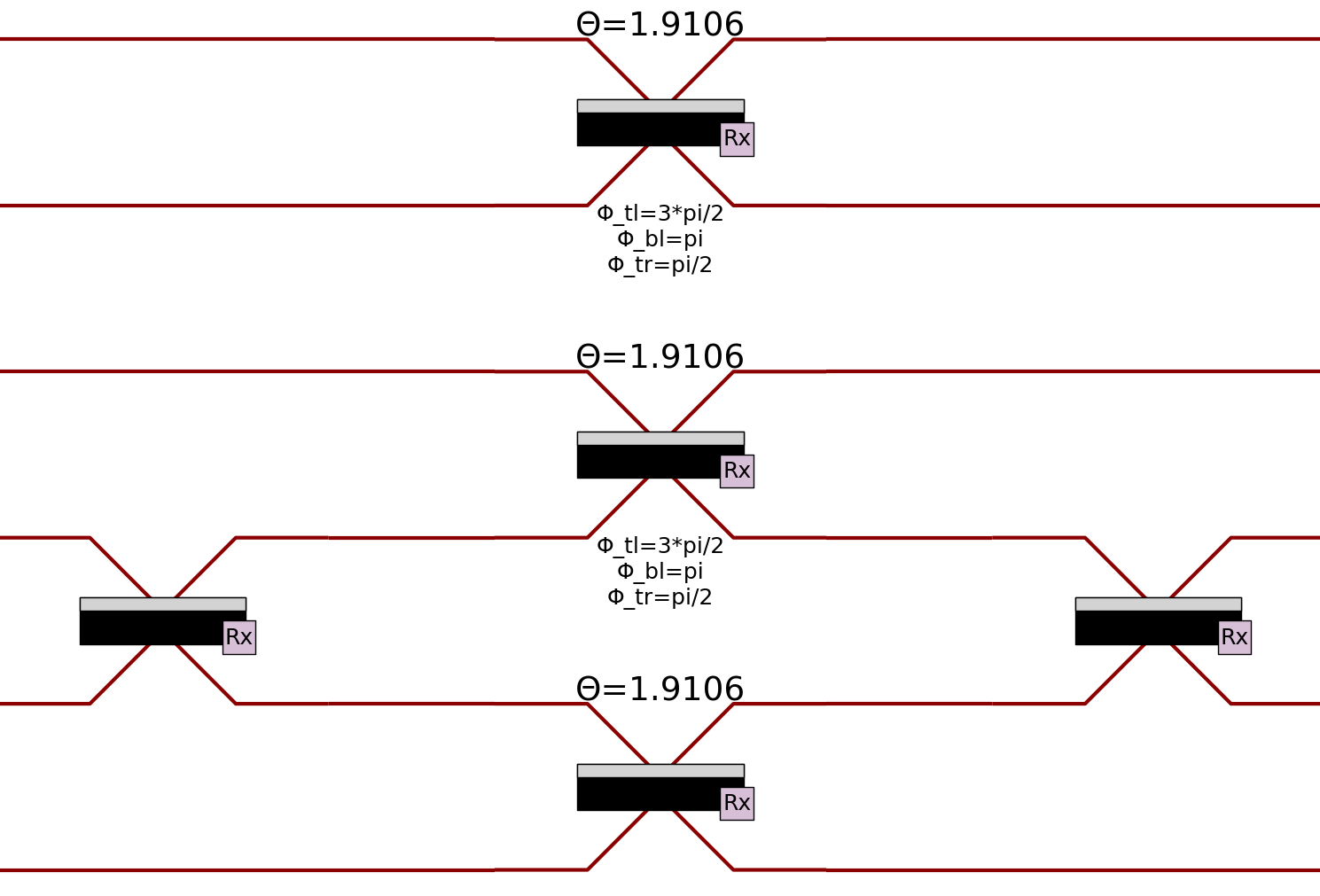
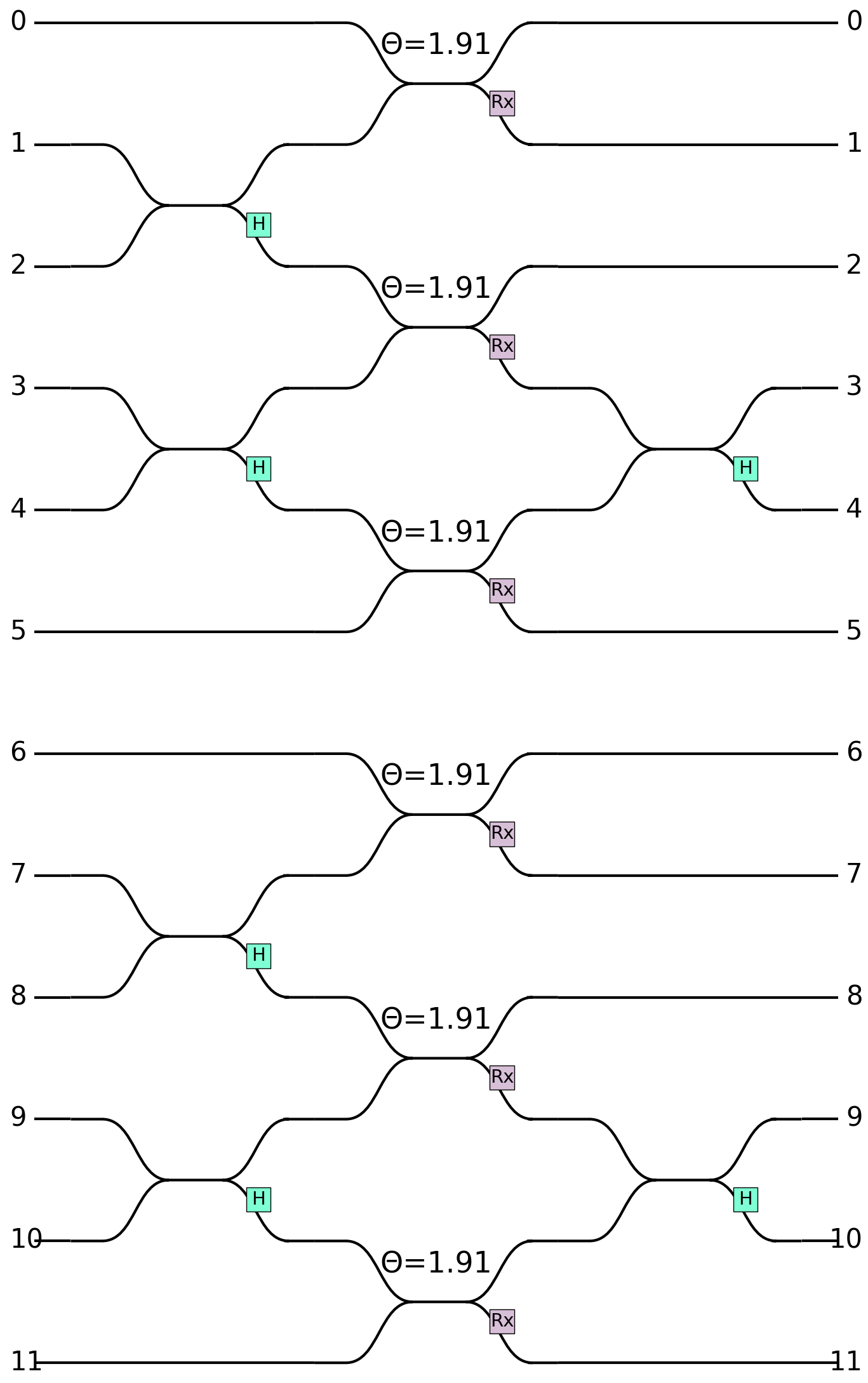
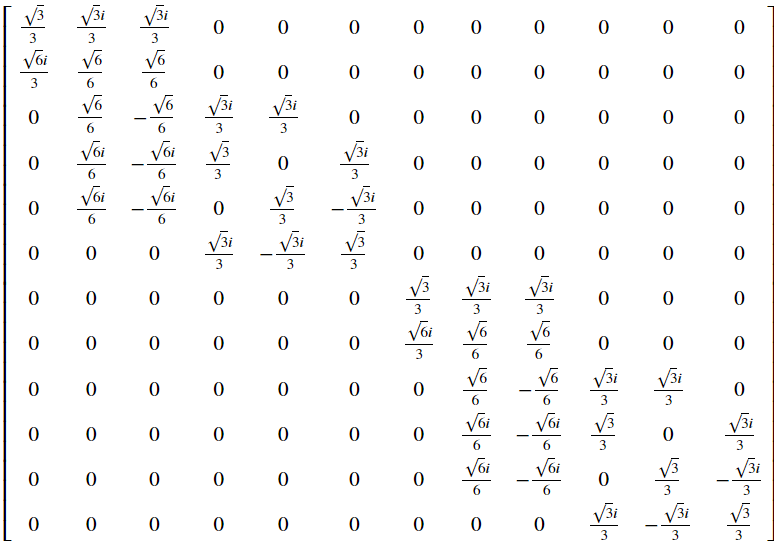
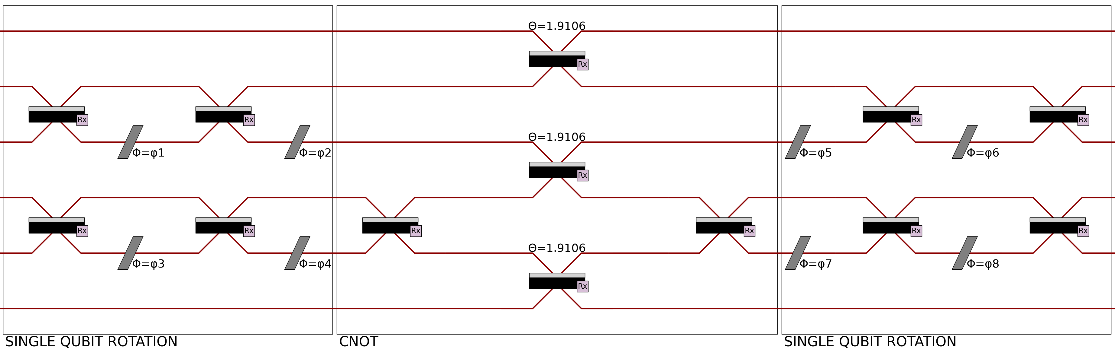
We use the linear optical circuit of the original paper [13] which was first introduced in [67]. The circuit has optical modes, consists of beam splitters, tunable phase shifters and single-photon detectors, and is shown in Figure 15. This circuit is essentially a 2-qubit circuit where qubits and are path encoded respectively in mode pairs and (here mode numbering is from to , from top to bottom). Modes and are auxiliary modes. The circuit consists of two parts. The first part being the central beam splitters in Figure 15, together with the beam splitters to the left and right of these central beam splitters, and which act on modes and . The central beam splitters have reflectivity , whereas the two to the left and right of the central ones have reflectivity . These beam splitters are used, together with modes and , to apply a gate to qubits and [46]. This is successful with probability under post-selection. The second part of the circuit consists of the remaining beam splitters and phase shifters, and is used to implement arbitrary single qubit rotations on qubits and . All phase shifters have tunable phase shifts, and all beam splitters have reflectivity .
Simulation.
Our strategy for the simulation of the VQE is as follows. We first compute the output state vector of the linear optical circuit, which depends on the phase shifters parameters [13], for some random initial configuration of these parameters. This enables the evaluation of the Rayleigh-Ritz quotient in Equation 18. Then, we proceed to minimise this quantity by using the Nelder-Mead minimisation algorithm [68].
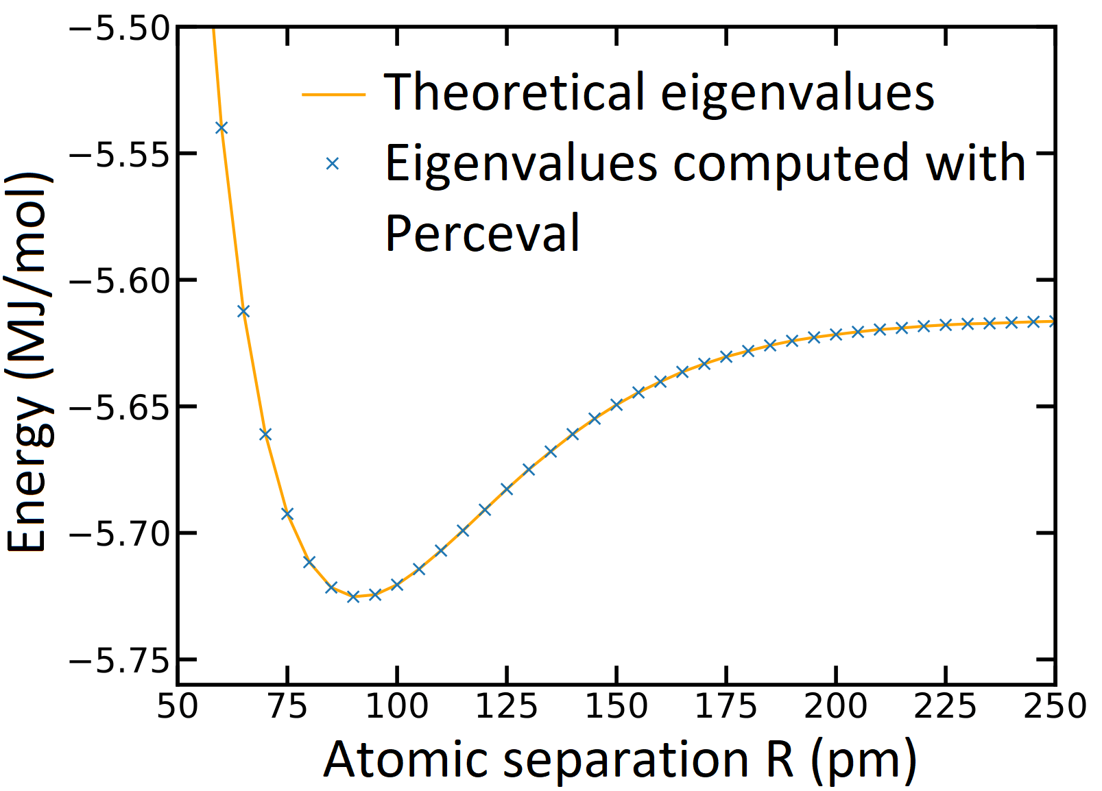
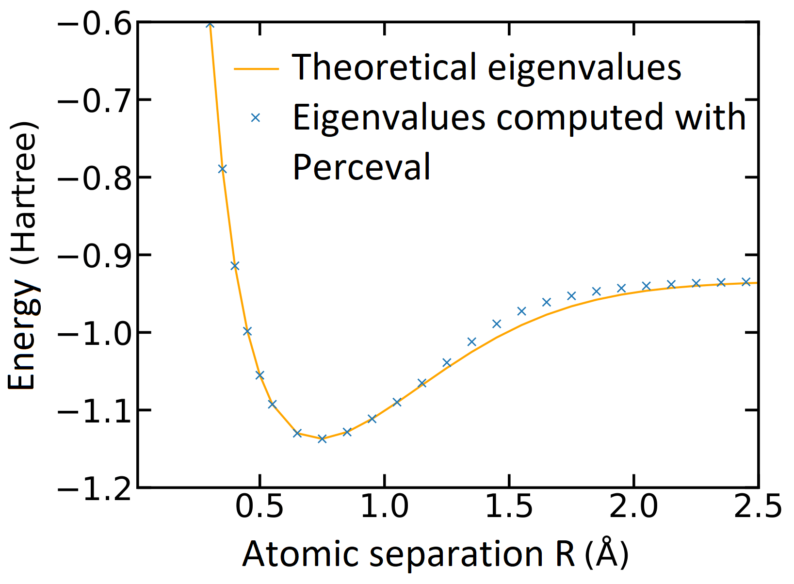
Using these techniques, we computed the ground-state molecular energies for the Hamiltonians of three different experiments [13] [69] [70]. In all these experiments, we used the circuit of Figure 15 to compute the output states . In line with the VQE algorithm, at each iteration we produce a different by tuning the angles of the phase shifters of the circuit in Figure 15. To test the validity of our techniques, we computed the theoretical ground-state molecular energies of the Hamiltonians of each of the 3 experiments. This was done with the NumPy [71] linear algebra package. A plot of these energies computed both theoretically and with Perceval is shown in Figure 16.
the Hamiltonian given in [13].
the Hamiltonian given in [69].
the Hamiltonian given in [70].
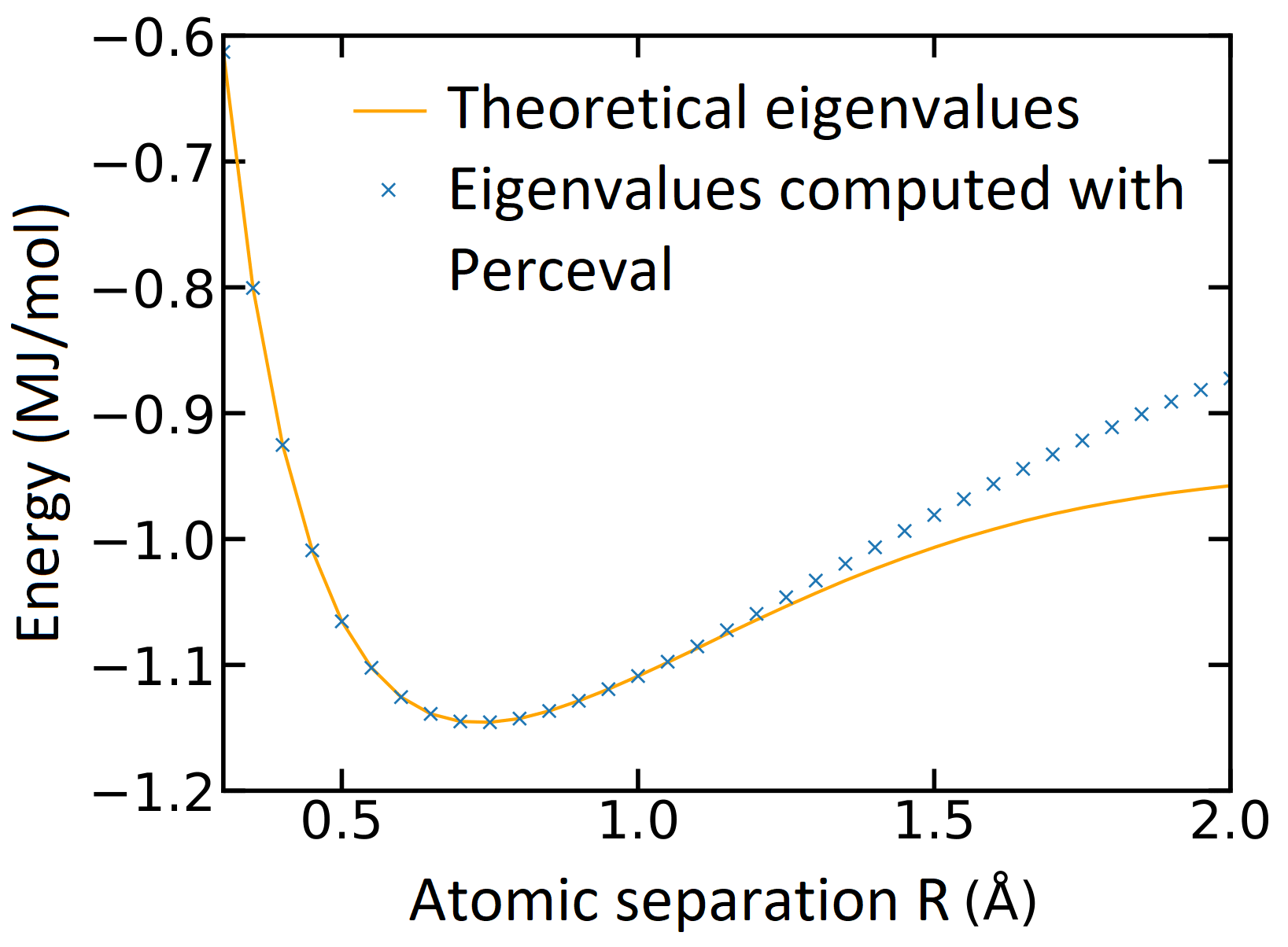
The circuit of Figure 15 was originally used in [13] to compute the ground-state energies of the Hamiltonian in Figure 16(a). We observe a very good overlap between theoretical and computed energies, indicating that the Perceval simulation was succesful. In [69, 70], different circuits than that of Figure 15 were used for computing the ground-state energies. Nevertheless, and in order to explore the expressivity [65] of the circuit of Figure 15, we computed and plotted in 16(b),16(c) the results of ground-state energy computations of the Hamitonians in [69, 70] using a VQE with the circuit of Figure 15. Our results in Figures 16(b),16(c) indicate in general a good overlap between theoretical and computed energies, with the deviations between theoretical and computed energies probably due to the fact that the circuit of Figure 15 is not expressive enough to give better accuracies.
4.6 Quantum Machine Learning
4.6.1 Introduction
Linear optics has proven to be a fascinating playground for exploring the advantages offered by quantum devices over their classical counterparts. For example, as discussed in Section 4.2, Boson Sampling [28], shows how a quantum device composed only of single photons, linear optical circuits, and single-photon detectors, can perform a computational task which quickly becomes unfeasible for the most powerful classical computers.
In [14], the authors show how linear optical circuits, similar to those used in Boson Sampling, can be used to solve other problems of more practical use than sampling. The basic idea is, following the work of [72, 73] for qubit-based quantum circuits, to encode data points onto the angles of phase shifters of a universal linear optical circuit. Effectively, this allows a non-linear manipulation of these data points. Indeed, this encoding of the data points allows to express the expectation value of some observable, computed using the linear optical circuit, as a Fourier series
| (20) |
of the data points [14]. The Fourier series, being a well known universal (periodic) function approximator, can be used for a variety of tasks, including approximating the solution of differential equations, which we will study here.
Interestingly, where is the number of photons inputted into the linear optical circuit [14]; meaning that the expressivity of the Fourier series – how well it can approximate a given function – depends (among other things) on the number of input photons of the linear optical circuit.
In the coming sections, we give an example of a quantum machine learning algorithm, using the above encoding, which solves a differential equation.
4.6.2 Expression of Photonic Quantum Circuit Expectation Values as Fourier Series
We focus on constructing a universal function approximator of a one-dimensional function with a photonic quantum device of photons and modes. This device consists of the following components: sources of single photons, -mode universal linear optical circuits, and number-resolving single-photon detectors [74]. Linear optical circuits can be configured to implement unitary matrices . A linear optical circuit is called universal if it can implement any such unitary [35]. The single photon sources produce input Fock states of the form , where is the number of photons in mode , and . The Fock space of photons in modes is isomorphic to the Hilbert space , with [28]. This isomorphism, together with a homomorphism from to (the and -dimensional unitary groups) detailed in [28], allows to understand the action of the unitary implemented by the linear optical circuit as an unitary acting on the input Fock state. In the rest of this section, as in [14], we will work with these unitary matrices when computing the universal function approximator.
The circuit architecture of [14] implements the unitary transformation
| (21) |
The phase shift operator incorporates the dependency of the function we wish to approximate. It is sandwiched between two universal linear optical circuits and . The parameters (angles of beam splitters and phase shifters of the linear optical circuits) and are tunable to enable training of the circuit, .
Let be the input state consisting of photons where is the number of photons in input mode . Consider the operator , given by
| (22) |
where the sum is taken over all possible Fock states of photons in modes, and some tunable set of parameters. The expectation value
| (23) |
of with respect to the output state of the linear optical circuit can be computed by measuring the output modes of this circuit using number-resolving detectors.
can be rewritten as the following Fourier series [14]
| (24) |
where is the frequency spectrum one can reach with incoming photons and are the Fourier coefficients. Hence this specific architecture can be used as a universal function approximator.
4.6.3 Application to Differential Equation Solving
The most general form of a differential equation verified by a function is
| (25) |
being an operator acting on , its derivatives and .
Given such an expression, we wish to optimise the parameters such that is a good approximation to a solution . More precisely, in this Quantum Machine Learning task, we aim at minimising a loss function whose value is related to the closeness of our approximator to a solution. This is done via a classical optimisation of the quantum free parameters , yielding ideally in the end
| (26) |
For the solving of differential equations, the loss function described in [75] consists of two terms
| (27) |
The first term corresponds to the differential equation which has been discretised over a set of points :
| (28) |
where for . The second term is associated to the initial conditions of our desired solution. It is defined as
| (29) |
where is the weight granted to the boundary condition and is given by , for some initial data point . These functions will be applied to the iterated approximations .
4.6.4 Perceval Implementation1919footnotemark: 19
2020footnotetext: This implementation is accompanied by a notebook.Our aim is to reproduce some of the results of [75], where the authors use so-called differentiable quantum circuits, together with the classical optimisation BFGS method of SciPy [76], to provide an approximation to the solution of the nonlinear differential equation
| (30) |
with , and boundary condition . The analytical solution of this differential equation is
| (31) |
Here, we solve this differential equation using the linear optical circuit architectures of Section 4.6.2 simulated in Perceval, together with classical optimisation. Note that the authors of [75] use Chebyshev polynomials as universal function approximators, whereas here we will use the Fourier series.
In our Perceval implementation, is chosen empirically as , granting sufficient weight to the boundary condition. Concerning the parameters, each one of them is sampled uniformly randomly in the interval , which is also empirically chosen. One could tune these parameters as well for greater accuracy, at the cost of a considerably slower minimisation procedure. The number of modes is taken to be equal to the number of photons . Differentiation is numerically conducted, , taken as . The discretised version of the loss function is taken on a grid of points, uniformly spaced between and .
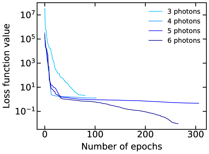
Results are shown for various photon numbers in Figure 17(a), demonstrating the increase in expressivity of the quantum circuit with growing . The converged solution for input photons provides a convincing approximation to the analytical solution. Increasing the number of photons further should yield even more accurate results, allowing for the realisation of more complex Quantum Machine Learning tasks.
A common indicator of the performance of a machine learning algorithm is the convergence of its loss function [77]. Confirming the results from Figure 17(a), additional photons allow us to reach lower values of the loss function, as shown in Figure 17(b). However this results in a longer convergence time due to an increased number of tunable parameters. Further details concerning the simulation in Perceval can be found in the documentation.

To summarise, we have used Perceval to simulate linear optical circuits providing universal function approximators [14], and shown that these can be used together with techniques from Quantum Machine Learning to accurately compute the solutions of differential equations. The accuracy of these function approximators depends, among other things, on the number of input photons of the linear optical circuits. An interesting future direction we aim to pursue is using Perceval and our developed techniques to solve other types of differential equations of significant practical interest [78, 79].
5 Conclusion
Perceval is a unique framework dedicated to linear optics and photonic quantum computing. This white paper has aimed to provide an overview of the platform, the motivations for its development, its structure and main features, and to give a variety of examples of Perceval in action. These examples are intended to be illustrative of some of the immediate uses of the platform.
Perceval’s simulation back-ends are optimised to run on local desktop devices, with extensions for HPC clusters. They can be used to run computational experiments to fine-tune algorithms, compare with experimental data from actual experiments and photonic quantum computing platforms, and can reproduce published articles in few lines of code.
Perceval is intended to be accessible to physicists, both experimental and theoretical, and computer scientists alike, with a goal of providing a bridge between these communities. With the intention of keeping a strong connection between software and hardware for photonic quantum computing, a major focus of future development will be on the continued development of realistic noise-models, that can describe with increasing accuracy the functioning of specific hardware components.
Perceval allows users to design algorithms and linear optical circuits through a large collection of predefined components. The collection of algorithms described here are available and presented as tutorials in the documentation. This is an open source project, with a modular architecture, and is welcoming of contributions from the community.
It is intended that future versions of Perceval will include more optimised simulators, noisy simulators, features for working with density matrices and cluster states, more advanced features and options for detectors to cover both threshold and photon-number resolving detectors, as well as features for treating circuits with feedforward.
Acknowledgements
The authors wish to thank Mario Valdiva for invaluable technical support, Arno Ricou for code and discussions on variational algorithms, and Jeanne Bourgeois, William Howard, Rayen Mahjoub, and Bechara Nasr, whose internships nourished early developments on the way to this paper. Finally, the authors would like to thank N. Quesada and the referees for their very valuable feedback that has greatly improved the quality of the paper.
References
- [1] Shor, P., “Algorithms for quantum computation: discrete logarithms and factoring,” in Proceedings 35th Annual Symposium on Foundations of Computer Science, pp. 124–134. IEEE, Nov., 1994.
- [2] Grover, L.K., “A fast quantum mechanical algorithm for database search,” in Proceedings of the twenty-eighth annual ACM symposium on Theory of Computing, STOC ’96, pp. 212–219. Association for Computing Machinery, July, 1996.
- [3] Preskill, J., “Quantum computing in the NISQ era and beyond,” Quantum 2, 79 (2018).
- [4] Preskill, J., “Quantum computing and the entanglement frontier,” arXiv:1203.5813 [quant-ph] (2011).
- [5] Arute, F., Arya, K., Babbush, R., Bacon, D. et al, “Quantum supremacy using a programmable superconducting processor,” Nature 574, 505–510 (2019).
- [6] Zhong, H.S., Wang, H., Deng, Y.H., Chen, M.C. et al, “Quantum computational advantage using photons,” Science 370, 1460–1463 (2020).
- [7] Wu, Y., Bao, W.S., Cao, S., Chen, F. et al, “Strong quantum computational advantage using a superconducting quantum processor,” Physical Review Letters 127, 180501 (2021).
- [8] Zhong, H.S., Deng, Y.H., Qin, J., Wang, H. et al, “Phase-programmable Gaussian Boson Sampling using stimulated squeezed light,” Physical Review Letters 127, 180502 (2021). Publisher: American Physical Society.
- [9] Madsen, L.S., Laudenbach, F., Askarani, M.F., Rortais, F. et al, “Quantum computational advantage with a programmable photonic processor,” Nature 606, 75–81 (2022).
- [10] Nikolopoulos, G.M. and Brougham, T., “Decision and function problems based on Boson Sampling,” Physical Review A 94, 012315 (2016).
- [11] Nikolopoulos, G.M., “Cryptographic One-Way Function based on Boson Sampling,” Quantum Information Processing 18, 259 (2019).
- [12] Banchi, L., Fingerhuth, M., Babej, T., Ing, C. and Arrazola, J.M., “Molecular docking with Gaussian Boson Sampling,” Science Advances 6, eaax1950 (2020).
- [13] Peruzzo, A., McClean, J., Shadbolt, P., Yung, M.H. et al, “A variational eigenvalue solver on a photonic quantum processor,” Nature Communications 5, 4213 (2014).
- [14] Gan, B.Y., Leykam, D. and Angelakis, D.G., “Fock State-enhanced expressivity of Quantum Machine Learning models,” in Conference on Lasers and Electro-Optics, p. JW1A.73. Optica Publishing Group, 2021.
- [15] Farhi, E., Goldstone, J. and Gutmann, S., “A Quantum Approximate Optimization Algorithm,” arXiv:1411.4028 [quant-ph] (2014).
- [16] Bharti, K., Cervera-Lierta, A., Kyaw, T.H., Haug, T. et al, “Noisy intermediate-scale quantum algorithms,” Rev. Mod. Phys. 94, 015004 (2022).
- [17] Cao, Y., Romero, J., Olson, J.P., Degroote, M. et al, “Quantum chemistry in the age of quantum computing,” Chemical Reviews 119, 10856–10915 (2019).
- [18] McArdle, S., Endo, S., Aspuru-Guzik, A., Benjamin, S.C. and Yuan, X., “Quantum computational chemistry,” Rev. Mod. Phys. 92, 015003 (2020).
- [19] Jiang, Z., Sung, K.J., Kechedzhi, K., Smelyanskiy, V.N. and Boixo, S., “Quantum algorithms to simulate many-body physics of correlated fermions,” Phys. Rev. Applied 9, 044036 (2018).
- [20] Davoudi, Z., Hafezi, M., Monroe, C., Pagano, G. et al, “Towards analog quantum simulations of lattice gauge theories with trapped ions,” Phys. Rev. Research 2, 023015 (2020).
- [21] Vikstål, P., Grönkvist, M., Svensson, M., Andersson, M. et al, “Applying the Quantum Approximate Optimization Algorithm to the tail-assignment problem,” Phys. Rev. Applied 14, 034009 (2020).
- [22] Zhu, L., Tang, H.L., Barron, G.S., Calderon-Vargas, F.A. et al, “An adaptive quantum approximate optimization algorithm for solving combinatorial problems on a quantum computer,” arXiv.2005.10258 [quant-ph] (2020).
- [23] Schuld, M., Brádler, K., Israel, R., Su, D. and Gupt, B., “Measuring the similarity of graphs with a Gaussian Boson sampler,” Phys. Rev. A 101, 032314 (2020).
- [24] Huang, H.Y., Broughton, M., Cotler, J., Chen, S. et al, “Quantum advantage in learning from experiments,” arXiv.2112.00778 [quant-ph] (2021).
- [25] Knill, E., Laflamme, R. and Milburn, G.J., “A scheme for efficient quantum computation with linear optics,” Nature 409, 46–52 (2001).
- [26] Kieling, K., Rudolph, T. and Eisert, J., “Percolation, renormalization, and quantum computing with nondeterministic gates,” Physical Review Letters 99, 130501 (2007).
- [27] Bartolucci, S., Birchall, P., Bombin, H., Cable, H. et al, “Fusion-based quantum computation,” arXiv:2101.09310 [quant-ph] (2021).
- [28] Aaronson, S. and Arkhipov, A., “The computational complexity of linear optics,” in Proceedings of the forty-third annual ACM symposium on Theory of computing, STOC ’11, pp. 333–342. Association for Computing Machinery, June, 2011.
- [29] Killoran, N., Izaac, J., Quesada, N., Bergholm, V. et al, “Strawberry Fields: A software platform for photonic quantum computing,” Quantum 3, 129 (2019).
- [30] Fingerhuth, M., Babej, T. and Wittek, P., “Open source software in quantum computing,” PLOS ONE 13, e0208561 (2018).
- [31] tA v, A., ANIS, M.S., Abby-Mitchell, Abraham, H. et al, “Qiskit: An Open-source Framework for Quantum Computing,” 2021.
- [32] Aguado, D.G., Gimeno, V., Moyano-Fernández, J.J. and Garcia-Escartin, J.C., “QOptCraft: A Python package for the design and study of linear optical quantum systems,” arXiv.2108.06186 [quant-ph] (2021).
- [33] Kok, P., Munro, W.J., Nemoto, K., Ralph, T.C. et al, “Linear optical quantum computing with photonic qubits,” Rev. Mod. Phys. 79, 135–174 (2007).
- [34] Kok, P. and Lovett, B.W., “Introduction to optical quantum information processing,”. Cambridge University Press, 2010.
- [35] Reck, M., Zeilinger, A., Bernstein, H.J. and Bertani, P., “Experimental realization of any discrete unitary operator,” Phys. Rev. Lett. 73, 58–61 (1994).
- [36] Clements, W.R., Humphreys, P.C., Metcalf, B.J., Kolthammer, W.S. and Walmsley, I.A., “Optimal design for universal multiport interferometers,” Optica 3, 1460–1465 (2016).
- [37] Chekhova, M. and Banzer, P., “Polarization of Light: In Classical, Quantum, and Nonlinear Optics,”. De Gruyter, 2021.
- [38] Valiant, L.G., “The complexity of computing the permanent,” Theoretical Computer Science 8, 189–201 (1979).
- [39] Spedalieri, F., Lee, H., Lee, H., Dowling, J. and Dowling, J., “Linear optical quantum computing with polarization encoding,” in Frontiers in Optics (2005), paper LMB4, p. LMB4. Optica Publishing Group, Oct., 2005.
- [40] Clifford, P. and Clifford, R., “The classical complexity of Boson Sampling,” in Proceedings of the 2018 Annual ACM-SIAM Symposium on Discrete Algorithms (SODA), Proceedings, pp. 146–155. Society for Industrial and Applied Mathematics, Jan., 2018.
- [41] Glynn, D.G., “The permanent of a square matrix,” European Journal of Combinatorics 31, 1887–1891 (2010).
- [42] Clifford, P. and Clifford, R., “Faster classical Boson Sampling,” arXiv:2005.04214 [quant-ph] (2020).
- [43] Ryser, H.J., “Combinatorial mathematics,”, vol. 14. American Mathematical Society, 1963.
- [44] Gupt, B., Izaac, J. and Quesada, N., “The Walrus: a library for the calculation of hafnians, Hermite polynomials and Gaussian boson sampling,” Journal of Open Source Software 4, 1705 (2019).
- [45] Heurtel, N., Mansfield, S., Senellart, J. and Valiron, B., “Strong Simulation of Linear Optical Processes,” arXiv:2206.10549 [quant-ph] (2022).
- [46] Ralph, T.C., Langford, N.K., Bell, T.B. and White, A.G., “Linear optical controlled-NOT gate in the coincidence basis,” Physical Review A 65, 062324 (2002).
- [47] Hong, C.K., Ou, Z.Y. and Mandel, L., “Measurement of subpicosecond time intervals between two photons by interference,” Physical Review Letters 59, 2044–2046 (1987). Publisher: American Physical Society.
- [48] Santori, C., Fattal, D., Vučković, J., Solomon, G.S. and Yamamoto, Y., “Indistinguishable photons from a single-photon device,” Nature 419, 594–597 (2002).
- [49] Giesz, V., Cavity-enhanced photon-photon interactions with bright quantum dot sources. Theses, Université Paris Saclay (COmUE), Dec., 2015.
- [50] Mezher, R. and Mansfield, S., “Assessing the quality of near-term photonic quantum devices,” arXiv:2202.04735 [quant-ph] (2022).
- [51] Brualdi, R.A. and Ryser, H.J., “Combinatorial Matrix Theory,”. Encyclopedia of Mathematics and its Applications. Cambridge University Press, 1991.
- [52] Aaronson, S. and Brod, D.J., “BosonSampling with lost photons,” Phys. Rev. A 93, 012335 (2016).
- [53] Arkhipov, A., “BosonSampling is robust against small errors in the network matrix,” Phys. Rev. A 92, 062326 (2015).
- [54] Kalai, G. and Kindler, G., “Gaussian noise sensitivity and Boson Sampling,” arXiv:1409.3093 [quant-ph] (2014).
- [55] Russell, N.J., Chakhmakhchyan, L., O’Brien, J.L. and Laing, A., “Direct dialling of Haar random unitary matrices,” New Journal of Physics 19, 033007 (2017).
- [56] Wang, H., Qin, J., Ding, X., Chen, M.C. et al, “Boson Sampling with 20 input photons and a 60-mode interferometer in a -dimensional Hilbert space,” Physical Review Letters 123, 250503 (2019).
- [57] Shchesnovich, V.S., “Universality of generalized bunching and efficient assessment of Boson Sampling,” Phys. Rev. Lett. 116, 123601 (2016).
- [58] Tichy, M.C., Mayer, K., Buchleitner, A. and Mølmer, K., “Stringent and efficient assessment of Boson-Sampling devices,” Phys. Rev. Lett. 113, 020502 (2014).
- [59] Walschaers, M., Kuipers, J., Urbina, J.D., Mayer, K. et al, “Statistical benchmark for BosonSampling,” New Journal of Physics 18, 032001 (2016).
- [60] Roy, T., Jiang, L. and Schuster, D.I., “Deterministic Grover search with a restricted oracle,” arXiv:2201.00091 [quant-ph] (2022).
- [61] Long, G.L., “Grover algorithm with zero theoretical failure rate,” Phys. Rev. A 64, 022307 (2001).
- [62] Kwiat, P.G., Mitchell, J.R., Schwindt, P.D.D. and White, A.G., “Grover’s search algorithm: An optical approach,” Journal of Modern Optics 47, 257–266 (2000).
- [63] Rivest, R.L., Shamir, A. and Adleman, L., “A Method for Obtaining Digital Signatures and Public-Key Cryptosystems,” Commun. ACM 21, 120–126 (1978).
- [64] Politi, A., Matthews, J.C.F. and O’Brien, J.L., “Shor’s quantum factoring algorithm on a photonic chip,” Science 325, 1221–1221 (2009).
- [65] Du, Y., Hsieh, M.H., Liu, T. and Tao, D., “Expressive power of parametrized quantum circuits,” Physical Review Research 2, 033125 (2020).
- [66] Hoeffding, W., “Probability inequalities for sums of bounded random variables,” in The collected works of Wassily Hoeffding, pp. 409–426. Springer, 1994.
- [67] Shadbolt, P.J., Verde, M.R., Peruzzo, A., Politi, A. et al, “Generating, manipulating and measuring entanglement and mixture with a reconfigurable photonic circuit,” Nature Photonics 6, 45–49 (2012).
- [68] Nelder, J.A. and Mead, R., “A Simplex Method for Function Minimization,” The Computer Journal 7, 308–313 (1965).
- [69] O’Malley, P.J.J., Babbush, R., Kivlichan, I.D., Romero, J. et al, “Scalable quantum simulation of molecular energies,” Phys. Rev. X 6, 031007 (2016).
- [70] Colless, J.I., Ramasesh, V.V., Dahlen, D., Blok, M.S. et al, “Computation of molecular spectra on a quantum processor with an error-resilient algorithm,” Phys. Rev. X 8, 011021 (2018).
- [71] Harris, C.R., Millman, K.J., van der Walt, S.J., Gommers, R. et al, “Array programming with NumPy,” Nature 585, 357–362 (2020).
- [72] Pérez-Salinas, A., Cervera-Lierta, A., Gil-Fuster, E. and Latorre, J.I., “Data re-uploading for a universal quantum classifier,” Quantum 4, 226 (2020).
- [73] Schuld, M., Sweke, R. and Meyer, J.J., “Effect of data encoding on the expressive power of variational quantum-machine-learning models,” Phys. Rev. A 103, 032430 (2021).
- [74] Hadfield, R.H., “Single-photon detectors for optical quantum information applications,” Nature Photonics 3, 696–705 (2009).
- [75] Kyriienko, O., Paine, A.E. and Elfving, V.E., “Solving nonlinear differential equations with differentiable quantum circuits,” Physical Review A 103, 052416 (2021).
- [76] Virtanen, P., Gommers, R., Oliphant, T.E., Haberland, M. et al, “SciPy 1.0: Fundamental Algorithms for Scientific Computing in Python,” Nature Methods 17, 261–272 (2020).
- [77] Raschka, S. and Mirjalili, V., “Python machine learning: Machine learning and deep learning with Python, scikit-learn, and TensorFlow 2,”. Packt Publishing Ltd, 2019.
- [78] Widder, D.V., “The heat equation,”, vol. 67. Academic Press, 1976.
- [79] Constantin, P. and Foias, C., “Navier-stokes equations,”. University of Chicago Press, 2020.
Appendix A Examples Codes of the Back-ends and the Processor class
A.1 CliffordClifford2017
|1,0,0,0,0,1,2,0>
|0,1,1,1,1,0,0,0>
|0,0,4,0,0,0,0,0>
|1,0,0,0,0,3,0,0>
|1,0,0,0,1,1,1,0>
A.2 Naive
|1,0,1,0> -> |1,0,1,0>: p=0.11351, p.ampl.=(-0.23806+0.23841j)
|1,0,1,0> -> |1,0,0,1>: p=0.09711, p.ampl.=(0.30757+0.05013j)
|1,0,1,0> -> |0,1,1,0>: p=0.19920, p.ampl.=(-0.02982+0.44532j)
|1,0,1,0> -> |0,0,2,0>: p=0.11104, p.ampl.=(-0.33287-0.01555j)
A.3 SLOS
| state | probability |
| |1,0,1,0 | 0.18959 |
| |2,0,0,0 | 0.162852 |
| |0,0,1,1 | 0.158684 |
| |0,0,2,0 | 0.138282 |
| |0,0,0,2 | 0.117126 |
| |1,0,0,1 | 0.088445 |
| |0,1,1,0 | 0.075928 |
| |0,1,0,1 | 0.056393 |
| |0,2,0,0 | 0.01188 |
| |1,1,0,0 | 0.000819328 |
A.4 Processor and Algorithm
| state | count |
| |0,1,0,1,0,0 | 50000 |
Ratio of samples with 2 photons: 1
Gate performance: 1/9
state
count
|0,1,0,1,0,0
50000
Ratio of samples with 2 photons: 1/4
Gate performance: 1/9
state
count
|0,1,0,1,0,0
47347
|0,0,1,1,0,0
2653
Ratio of samples with 2 photons: 0.257315
Gate performance: 0.108027