Monarch: Expressive Structured Matrices for Efficient and Accurate Training

Abstract

Large neural networks excel in many domains, but they are expensive to train and fine-tune. A popular approach to reduce their compute/memory requirements is to replace dense weight matrices with structured ones (e.g., sparse, low-rank, Fourier transform). These methods have not seen widespread adoption (1) in end-to-end training due to unfavorable efficiency–quality tradeoffs, and (2) in dense-to-sparse fine-tuning due to lack of tractable algorithms to approximate a given dense weight matrix. To address these issues, we propose a class of matrices (Monarch) that is hardware-efficient (they are parameterized as products of two block-diagonal matrices for better hardware utilization) and expressive (they can represent many commonly used transforms). Surprisingly, the problem of approximating a dense weight matrix with a Monarch matrix, though nonconvex, has an analytical optimal solution. These properties of Monarch matrices unlock new ways to train and fine-tune sparse and dense models. We empirically validate that Monarch can achieve favorable accuracy–efficiency tradeoffs in several end-to-end sparse training applications: speeding up ViT and GPT-2 training on ImageNet classification and Wikitext-103 language modeling by 2$\times$ with comparable model quality, and reducing the error on PDE solving and MRI reconstruction tasks by 40%. In sparse-to-dense training, with a simple technique called “reverse sparsification,” Monarch matrices serve as a useful intermediate representation to speed up GPT-2 pretraining on OpenWebText by 2$\times$ without quality drop. The same technique brings 23% faster BERT pretraining than even the very optimized implementation from Nvidia that set the MLPerf 1.1 record. In dense-to-sparse fine-tuning, as a proof-of-concept, our Monarch approximation algorithm speeds up BERT fine-tuning on GLUE by 1.7$\times$ with comparable accuracy.

1 Introduction

Large neural networks excel in many domains, but their training and fine-tuning demand extensive computation and memory [54]. A natural approach to mitigate this cost is to replace dense weight matrices with structured ones, such as sparse & low-rank matrices and the Fourier transform. However, structured matrices (which can be viewed as a general form of sparsity) have not yet seen wide adoption to date, due to two main challenges. (1) In the end-to-end (E2E) training setting, they have shown unfavorable efficiency–quality tradeoffs. Model efficiency refers how efficient these structured matrices are on modern hardware (e.g., GPUs). Model quality (performance on tasks) is determined by how expressive they are (e.g., can they represent commonly used transforms such as convolution or Fourier/cosine transforms that encode domain-specific knowledge). Existing structured matrices are either not hardware-efficient, or not expressive enough. (2) In the setting of dense-to-sparse (D2S) fine-tuning of pretrained models, a long-standing problem for most classes of structured matrices is the lack of tractable algorithms to approximate dense pretrained weight matrices [79].

Sparse matrices have seen advances in training deep learning models (e.g., pruning [44], lottery tickets [30]), but most work on (entrywise) sparsification focuses on reducing training or inference FLOPs, which do not necessarily map to E2E training time on modern hardware (e.g., GPUs). In fact, most sparse training methods slow down training in wall-clock time [33, 48]. Moreover, sparse matrices are not able to represent commonly used transforms such as convolution and the Fourier transform. Another class of structured matrices, such as Fourier, sine/cosine, Chebyshev, are used in specialized domains such as PDE solving [100] and medical imaging [49]. However, they are difficult to use in E2E training since only specific instances of these structured matrices have fast GPU implementations (e.g., FFT). Moreover, their applications requires domain expertise to hand-pick the right transforms. Generalizations of these transforms (e.g., Toeplitz-like [95], orthogonal polynomial transforms [25], low-displacement rank [53], quasi-separable [27]), though learnable, often lack efficient implementation on GPUs [98] for E2E training as well. In addition, they have no known tractable algorithm to approximate a given dense matrix [79], making them difficult to use in D2S fine-tuning.

E2E training. The technical challenge in addressing the efficiency–quality tradeoff of structured matrices is to find a parameterization that is both efficient on block-oriented hardware (e.g., GPUs) and expressive (e.g., can represent many commonly used transforms). We propose a class of matrices called Monarch, parameterized as products of two block-diagonal matrices (up to permutation), to address this challenge. This parameterization leverages optimized batch-matrix-multiply (BMM) routines on GPUs, yielding up to 2$\times$ speedup compared to dense matrix multiply (Section 5.1.1). We show that the class of Monarch matrices contains the class of butterfly matrices [80, 12], which can represent any low-depth arithmetic circuits in near optimal runtime and parameter size [13]. Monarch matrices inherit this expressiveness and thus can represent many fast transforms (e.g., Fourier, sine/cosine/Chebyshev transforms, convolution) (Proposition 3.2).

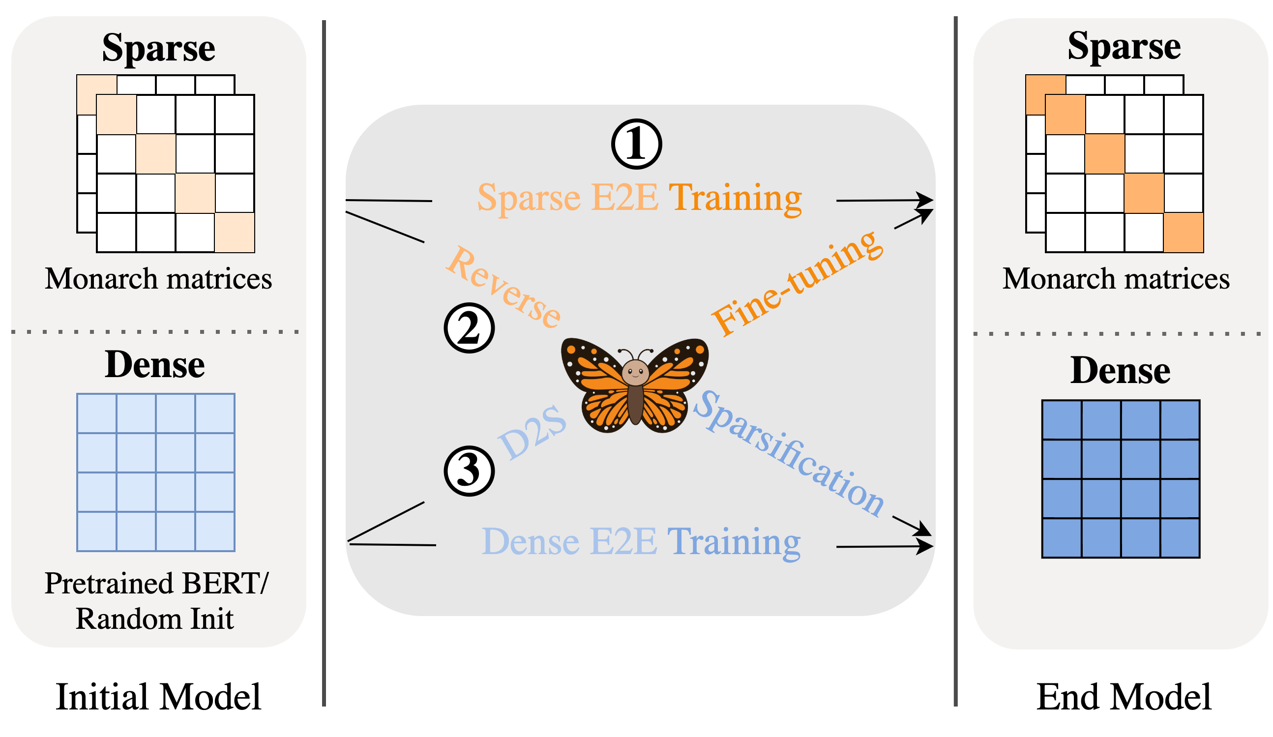
Figure 1: Monarch matrices unlock several ways to train sparse and dense models: end-to-end training a sparse (Monarch) model can be 2x faster than dense training thanks to its hardware efficiency; sparse-to-dense “reverse sparsification” can speed up training of large models such as GPT-2; and our dense-to-sparse Monarch projection algorithm can transfer knowledge from pretrained dense model to Monarch model and speed up BERT fine-tuning.

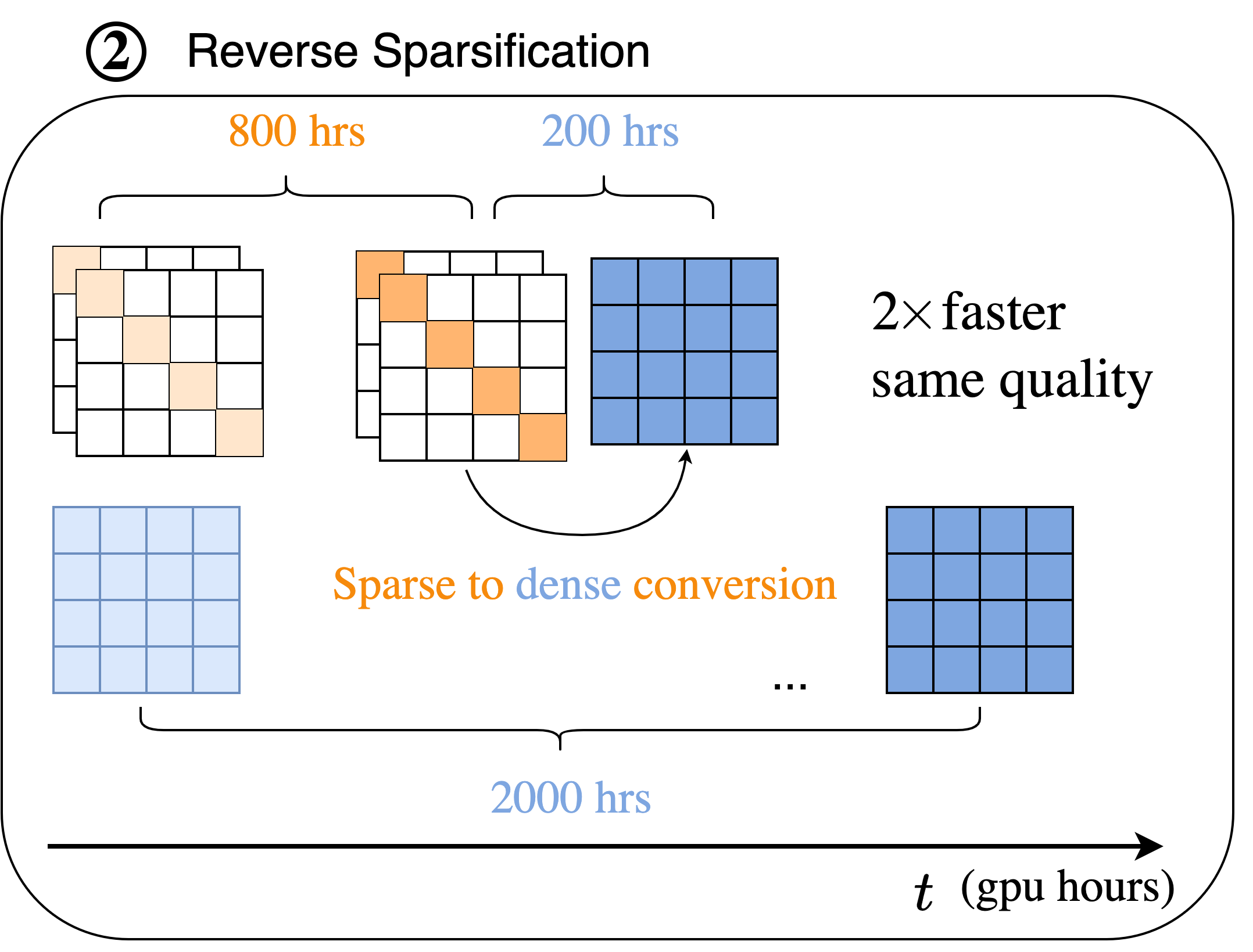
Figure 3: With the “reverse sparsification” process, Monarch matrices can speed up GPT-2 training by 2x.

Sparse-to-dense (S2D) training, aka “reverse sparsification”. The hardware-efficiency and expressiveness of Monarch matrices unlock a new way to train dense models: training with Monarch weight matrices for most of the time and then transitioning to dense weight matrices (Fig. 3). This technique can be used in cases where sparse training faces representation or optimization difficulties [28] or a dense model is necessary. One such application is language modeling on large datasets, where a massive number of parameters are required [54] to memorize the textual patterns [35]. Monarch matrices can serve as a fast intermediate representation to speed up the training process of the dense model.

D2S fine-tuning. While transitioning from sparse to dense matrices is easy, the reverse direction is challenging. The main technical difficulty is the projection problem: finding a matrix in a class of structured matrices that is the closest to a given dense matrix. Only a few specific classes of structured matrices have a tractable projection solution, such as entrywise sparse matrices (magnitude pruning [97]), low-rank matrices (the Eckart-Young theorem [26]), and orthogonal matrices (the orthogonal Procrustes problem [93]). For more expressive classes of structured matrices, projection remains a long-standing problem [79]. For example, De Sa et al. [16] show that all structured matrices (in the form of arithmetic circuits) can be written as products of sparse matrices, which can be represented as products of butterfly matrices [13]. There have been numerous heuristics proposed to project on the set of butterfly matrices or products of sparse matrices, based on iterative first-order optimization [63, 12, 55] or alternating minimization [67]. However, they lack theoretical guarantees. In contrast, we derive a projection algorithm for our Monarch parameterization and prove that it finds the optimal solution (Theorem 1). We also derive an algorithm to factorize matrices that are products of Monarch matrices (Section 3.4). These new algorithms allows us to easily finetune a pretrained model into a model with Monarch weight matrices (Section 5.3).

We validate our approach empirically in these three settings, showing that our Monarch matrix parameterization achieves a favorable efficiency–accuracy tradeoff compared to baselines on a wide range of domains: text, images, PDEs, MRI.

• In the E2E sparse training setting (Section 5.1), our Monarch matrices model trains 2$\times$ faster than dense models while achieving the same accuracy / perplexity on benchmark tasks (ViT on ImageNet classification, GPT-2 on Wikitext-103 language modeling). On scientific and medical tasks relying on hand-crafted fast transforms (PDE solving, MRI reconstruction), Monarch reduces the error by up to 40% at the same training speed compared to domain-specific Fourier-based methods.

• In the S2D training setting (Section 5.2), our “reverse sparsification” process with Monarch matrices speeds up GPT-2 pretraining on the large OpenWebText dataset by 2$\times$ compared to an optimized implementation from NVIDIA [94], with comparable upstream and downstream (text classification) quality. When applied to BERT pretraining, our method is 23% faster than the implementation from Nvidia that set the MLPerf [72] 1.1 record.

• In the D2S fine-tuning setting (Section 5.3), we show a proof of concept that our Monarch projection algorithm speeds up BERT fine-tuning. We project a pretrained BERT model to a Monarch matrix model and fine-tune on GLUE, with 2$\times$ fewer parameters, 1.7$\times$ faster fine-tuning speed, and similar average GLUE accuracy as the dense model.

2 Related Work and Background

2.1 Related Work

Sparse Training. Sparse training is an active research topic. There has been inspiring work along the line of compressing models such as neural network pruning and lottery tickets [44, 45, 30]. Pruning methods usually eliminate neurons and connections through iterative retraining [44, 45, 92] or at runtime [66, 23]. Although both Monarch and pruning methods aim to produce sparse models, we differ in our emphasis on overall efficiency, whereas pruning mostly focuses on inference efficiency and disregards the cost of finding the smaller model. Lottery tickets [30, 31, 32] are a set of small sub-networks derived from a larger dense network, which outperforms their parent networks in convergence speed and potentially in generalization. Monarch can be roughly seen as a class of manually constructed lottery tickets.

Structured Matrices. Structured matrices are those with subquadratic ($o(n^{2})$ for dimension $n\times n$) number of parameters and runtime. Examples include sparse and low-rank matrices, and fast transforms (Fourier, Chebyshev, sine/cosine, orthogonal polynomials). They are commonly used to replace the dense weight matrices of deep learning models, thus reducing the number of parameters and training/inference FLOPs. Large classes of structured matrices (e.g., Toeplitz-like [95], low-displacement rank [53], quasi-separable [27]) have been shown to be able to represent many commonly used fast transforms. For example, De Sa et al. [16] show that a simple divide-and-conquer scheme leads to a fast algorithm for a large class of structured matrices. Our work builds on butterfly matrices [80, 12], which have been shown to be expressive but remain hardware-inefficient. Pixelated butterfly [6] has attempted to make butterfly matrices more hardware-friendly, but at the cost of reduced expressiveness. Furthermore, it is not known if one can directly decompose a dense pretrained model to a model with butterfly weight matrices without retraining.

2.2 Butterfly Matrices

Our work builds on recent work on butterfly matrices. Dao et al. [12] introduced the notion of a butterfly matrix as a certain product of permuted block-diagonal matrices, inspired by the Cooley-Tukey fast Fourier transform algorithm [11]. They encode the divide-and-conquer structure of many fast multiplication algorithms. Dao et al. [13] showed that all structured matrices can be written as products of such butterfly matrices, and this representation has optimal memory and runtime complexity up to polylogarithmic factors. We now review these definitions (following [13]).

A butterfly factor of size $k$ (where $k$ is even) is a matrix of the form $\begin{bmatrix}\mathbf{D}_{1}&\mathbf{D}_{2}\\ \mathbf{D}_{3}&\mathbf{D}_{4}\end{bmatrix}$ where each $\mathbf{D}_{i}$ is a $\frac{k}{2}\times\frac{k}{2}$ diagonal matrix. We call this class of matrices $\mathcal{B}\mathcal{F}^{(k,k)}$.

A butterfly factor matrix of size $n$ and block size $k$ is a block diagonal matrix of $\frac{n}{k}$ butterfly factors of size $k$:

$$\mathrm{diag}\left(\mathbf{B}_{1},\mathbf{B}_{2},\ldots,\mathbf{B}_{\frac{n}{k}}\right),$$

where $\mathbf{B}_{i}\in\mathcal{B}\mathcal{F}^{(k,k)}$. We call this class of matrices $\mathcal{B}\mathcal{F}^{(n,k)}$.

Finally, a butterfly matrix of size $n=2^{s}$ is a matrix $\mathbf{M}$ that can be expressed as a product of butterfly factor matrices:

$$\mathbf{M}=\mathbf{B}_{n}\mathbf{B}_{n/2}\ldots\mathbf{B}_{2},$$

where each $\mathbf{B}_{i}\in\mathcal{B}\mathcal{F}^{(n,i)}$. We denote the set of size-$n$ butterfly matrices by $\mathcal{B}^{(n)}$. Equivalently, $\mathbf{M}$ can be written in the following form:

$$\mathbf{M}=\mathbf{B}_{n}\begin{bmatrix}\mathbf{M}_{1}&0\\ 0&\mathbf{M}_{2}\end{bmatrix},$$

where $\mathbf{B}_{n}\in\mathcal{B}\mathcal{F}^{(n,n)}$ and $\mathbf{M}_{1},\mathbf{M}_{2}\in\mathcal{B}^{(\frac{n}{2})}$.

Dao et al. [13] further introduce the kaleidoscope matrix hierarchy: the class $\mathcal{B}\mathcal{B}^{*(n)}$ is the set of matrices of the form $\mathbf{M}_{1}\mathbf{M}_{2}^{*}$ for $\mathbf{M}_{1},\mathbf{M}_{2}\in\mathcal{B}^{(n)}$, and the class $(\mathcal{B}\mathcal{B}^{*(n)})^{w}_{e}$ is the set of all matrices of the form $\left(\prod\limits_{i=1}^{w}\mathbf{M}_{i}\right)[1{:}n,1{:}n]$ where each $\mathbf{M}_{i}\in\mathcal{B}\mathcal{B}^{*(e\cdot n)}$. ($\mathbf{A}^{*}$ denotes the conjugate transpose of $\mathbf{A}$.) When the size $n$ is clear from context, we will omit the superscript ⁽ⁿ⁾ (i.e., just write $\mathcal{B},\mathcal{B}\mathcal{B}^{*}$, etc.). As shown by Theorem 1 of Dao et al. [13], the kaleidoscope hierarchy can represent any structured matrix with nearly-optimal parameters and runtime: if $\mathbf{M}$ is an $n\times n$ matrix such that multiplying any vector $v$ by $\mathbf{M}$ can be represented as a linear arithmetic circuit with depth $d$ and $s$ total gates, then $\mathbf{M}\in(\mathcal{B}\mathcal{B}^{*(n)})^{O(d)}_{O(s/n)}$.

3 Monarch: Definition & Algorithms

In Section 3.1, we introduce Monarch matrices, and describe how they relate to butterfly matrices. In Section 3.2 we show that the class of Monarch matrices is at least as expressive as the class of butterfly matrices, while admitting a practically efficient representation. In particular, many fast transforms (e.g., Fourier, convolution) can be represented as a Monarch matrix or as the product of two or four Monarch matrices (Proposition 3.2). In Section 3.3, we show how to project onto the set of Monarch matrices. This allows us to tractably approximate a given matrix (e.g., a dense pretrained weight matrix) with a Monarch matrix, unlocking new applications (cf. Section 5). In Section 3.4, we show how to recover the individual factors of the larger class of products of two Monarch matrices.

3.1 Monarch Parametrization for Square Matrices

Inspired by the 4-step FFT algorithm [3], we propose the class of Monarch matrices, each parametrized as the product of two block-diagonal matrices up to permutation:

Definition 3.1.

Let $n=m^{2}$. An $n\times n$ Monarch matrix has the form:

$$\mathbf{M}=\mathbf{P}\mathbf{L}\mathbf{P}^{\top}\mathbf{R},$$

where $\mathbf{L}$ and $\mathbf{R}$ are block-diagonal matrices, each with $m$ blocks of size $m\times m$, and $\mathbf{P}$ is the permutation that maps $[x_{1},\dots,x_{n}]$ to $[x_{1},x_{1+m},\dots,x_{1+(m-1)m},x_{2},x_{2+m},\dots,\newline x_{2+(m-1)m},\dots,x_{m},x_{2m},\dots,x_{n}]$.

We call this the Monarch parametrization. We denote the class of all matrices that can be written in this form as $\mathcal{M}^{(n)}$ (dropping the superscript when clear from context). Fig. 2 illustrates this parametrization.

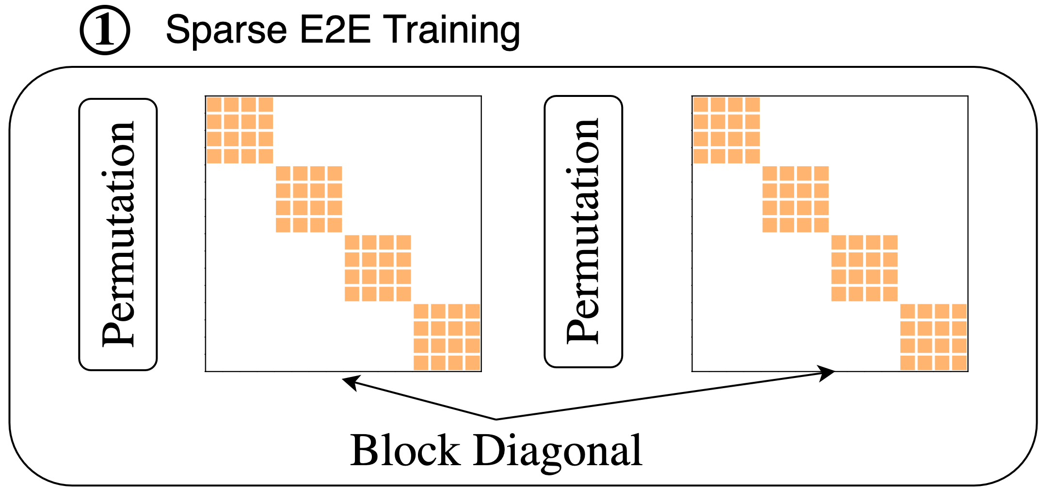
Figure 2: Monarch matrices are parametrized as products of two block-diagonal matrices up to permutation, allowing efficient multiplication algorithm that leverages batch matrix multiply.

We now provide more intuition for this parametrization and connect it to butterfly matrices. For ease of exposition, suppose $\mathbf{B}\in\mathcal{B}^{(n)}$ where $n$ is a power of 4. Then let $\mathbf{L}^{\prime}$ be obtained by multiplying together the first $\tfrac{\log_{2}n}{2}$ butterfly factor matrices in the butterfly factorization of $\mathbf{B}$, and $\mathbf{R}$ by multiplying together the last $\tfrac{\log_{2}n}{2}$ butterfly factor matrices. (We detail this more rigorously in Theorem 4.)

The matrix $\mathbf{R}$ is block-diagonal with $m=\sqrt{n}$ dense blocks, each block of size $m\times m$: $\mathbf{R}=\mathrm{diag}(\mathbf{R}_{1},\dots,\mathbf{R}_{m}).$

The matrix $\mathbf{L}^{\prime}$ is composed of $m\times m$ blocks of size $m\times m$, where each block is a diagonal matrix:

$$\mathbf{L}^{\prime}=\begin{bmatrix}\mathbf{D}_{11}&\ldots&\mathbf{D}_{1m}\\ \vdots&\ddots&\vdots\\ \mathbf{D}_{m1}&\ldots&\mathbf{D}_{mm}\\ \end{bmatrix}.$$

The matrix $\mathbf{L}^{\prime}$ can also be written as block-diagonal with the same structure as $\mathbf{R}$ after permuting the rows and columns. Specifically, let $\mathbf{P}$ be the permutation of Definition 3.1. We can interpret $\mathbf{P}$ as follows: it reshapes the vector $x$ of size $n$ as a matrix of size $m\times m$, transposes the matrix, then converts back into a vector of size $n$. Note that $\mathbf{P}=\mathbf{P}^{\top}$. Then we can write

$$\mathbf{L}=\mathbf{P}\mathbf{L}^{\prime}\mathbf{P}^{\top},\quad\text{where }\mathbf{L}=\mathrm{diag}(\mathbf{L}_{1},\dots,\mathbf{L}_{m}).$$

Hence, up to permuting rows and columns, $\mathbf{L}^{\prime}$ is also a block-diagonal matrix of $m$ dense blocks, each of size $m\times m$.

Thus we can write $\mathbf{B}=\mathbf{P}\mathbf{L}\mathbf{P}^{\top}\mathbf{R}$, where $\mathbf{L}$, $\mathbf{R}$, and $\mathbf{P}$ are as in Definition 3.1. So, $\mathbf{B}\in\mathcal{B}^{(n)}$ implies that $\mathbf{B}\in\mathcal{M}^{(n)}$.

Products of Monarch Matrices. Another important class of matrices (due to their expressiveness, cf. Proposition 3.2) is the class $\mathcal{M}\mathcal{M}^{*}$: matrices that can be written as $\mathbf{M}_{1}\mathbf{M}_{2}^{*}$ for some $\mathbf{M}_{1},\mathbf{M}_{2}\in\mathcal{M}$. Further, $(\mathcal{M}\mathcal{M}^{*})^{2}$ denotes the class of matrices that can be written $\mathbf{M}_{1}\mathbf{M}_{2}$ for $\mathbf{M}_{1},\mathbf{M}_{2}\in\mathcal{M}\mathcal{M}^{*}$.

Extension to Rectangular Matrices. In practice, we also want a way to parametrize rectangular weight matrices, and to increase the number of parameters of Monarch matrices to fit different applications (analogous to the rank parameter in low-rank matrices and the number of nonzeros in sparse matrices). We make the simple choice to increase the block size of the block-diagonal matrices in the Monarch parametrization, and to allow rectangular blocks. More details are in Appendix C.

3.2 Expressiveness and Efficiency

We remark on the expressiveness of Monarch matrices and their products (ability to represent many structured transforms), and on their computational and memory efficiency.

3.2.1 Expressiveness

As described in Section 3.1, any matrix $\mathbf{B}\in\mathcal{B}^{(n)}$ can be written in the Monarch butterfly representation, by simply condensing the $\log_{2}n$ total factors into two matrices. Thus, the Monarch butterfly representation is strictly more general than the original butterfly representation (as there also exist matrices in $\mathcal{M}^{(n)}$ but not $\mathcal{B}^{(n)}$). In other words, for a given size $n$, $\mathcal{M}\supset\mathcal{B}$; similarly $\mathcal{M}\mathcal{M}^{*}\supset\mathcal{B}\mathcal{B}^{*}$. In particular, Dao et al. [13] showed that the following matrix classes are contained in $\mathcal{B}\mathcal{B}^{*}$, which implies they are in $\mathcal{M}\mathcal{M}^{*}$ as well:

Proposition 3.2.

The matrix class $\mathcal{M}\mathcal{M}^{*}$ can represent convolution, Hadamard transform, Toeplitz matrices [37], and AFDF matrices [74]. The matrix class $(\mathcal{M}\mathcal{M}^{*})^{2}$ can represent the Fourier transform, discrete sine and cosine transforms (DST/DCT), the $(HD)^{3}$ [106] class, Fastfood [62], and ACDC matrices [74].

3.2.2 Efficiency

Parameters. A Monarch matrix $\mathbf{M}=\mathbf{P}\mathbf{L}\mathbf{P}^{\top}\mathbf{R}$ is described by $2n\sqrt{n}$ parameters: $\mathbf{L},\mathbf{R}$ both have $\sqrt{n}$ dense blocks of size $\sqrt{n}\times\sqrt{n}$, for a total parameter count of $n\sqrt{n}$ each. The permutation $\mathbf{P}$ is fixed, and thus doesn’t add any parameters. Speed. To multiply by $\mathbf{M}$, we need to multiply by a block diagonal matrix $\mathbf{R}$, permute, multiply by a block diagonal matrix $\mathbf{L}$, and finally permute. All four of these steps can be implemented efficiently. The total number of FLOPs is $O(n\sqrt{n})$, which is more the $O(n\log n)$ for a butterfly matrix. However, since we can leverage efficient block-diagonal multiplication (e.g., batch matrix multiply), Monarch multiplication is easy to implement and is fast in practice (2x faster than dense multiply, cf. Section 5).

3.3 Projection on the Set $\mathcal{M}$ of Monarch Matrices

Given our class of structured matrices, a natural question is the projection problem: finding a Monarch matrix that is the closest to a given dense matrix. We show that this problem has an analytical optimal solution, and show how to compute it efficiently. This allows us to project dense models to Monarch models, enabling D2S fine-tuning (Section 5.3).

We formalize the problem: for a given matrix $\mathbf{A}$, find

$$\operatorname*{argmin}\limits_{\mathbf{M}\in\mathcal{M}}\left\|{\mathbf{A}-\mathbf{M}}\right\|^{2}_{F}.$$ (1)

Even though this problem is nonconvex (as $\mathbf{M}$ is parametrized as the product of two matrices), in Theorem 1 we show that there exists an analytical solution (full proof in Appendix D). This is analogous to the Eckart-Young theorem that establishes that optimal low-rank approximation is obtained from the SVD [26].

Theorem 1.

Given an $n\times n$ matrix $\mathbf{A}$, there is an $O(n^{5/2})$-time algorithm that optimally solves the projection problem (1), and returns the Monarch factors $\mathbf{L}$ and $\mathbf{R}$.

We now derive this algorithm (Algorithm 1) by examining the structure of a Monarch matrix $\mathbf{M}$.

We first rewrite the steps of Monarch matrix-vector multiplication (i.e., computing $\mathbf{M}\mathbf{x}$). The main idea is to view the input $\mathbf{x}$, which is a vector of size $n=m^{2}$, as a 2D tensor of size $m\times m$. Then the two matrices $\mathbf{L}$ and $\mathbf{R}$ in the Monarch parametrization $\mathbf{M}=\mathbf{P}\mathbf{L}\mathbf{P}^{\top}\mathbf{R}$ correspond to batched matrix multiply along one dimension of $\mathbf{x}$, followed by batched matrix multiply along the other dimension of $\mathbf{x}$. Thus we view $\mathbf{x}$ as a 2D tensor of size $m\times m$, and each of $\mathbf{L}$ and $\mathbf{R}$ as a 3D tensor of size $m\times m\times m$.

Steps to multiply $\mathbf{x}$ by a Monarch matrix $\mathbf{M}=\mathbf{P}\mathbf{L}\mathbf{P}^{\top}\mathbf{R}$:

1. Multiply $\mathbf{R}$ by $\mathbf{x}$: $y_{kj}=\sum_{i}R_{kji}x_{ki}$, to obtain an output $\mathbf{y}$ that is a 2D tensor of size $m\times m$.

2. Multiply $\mathbf{P}\mathbf{L}\mathbf{P}^{\top}$ by $\mathbf{y}$: $z_{\ell j}=\sum_{k}L_{j\ell k}y_{kj}$, to obtain an output that is a 2D tensor of size $m\times m$.

3. Reshape $\mathbf{z}$ back into a vector of size $n$, and return this.

We can thus write the output $\mathbf{z}$ as $z_{\ell j}=\sum_{k,i}L_{j\ell k}R_{kji}x_{ki}$.
Since $\mathbf{M}=\mathbf{P}\mathbf{L}\mathbf{P}^{\top}\mathbf{R}$, we can write:

$$M_{\ell jki}=L_{j\ell k}R_{kji}.$$ (2)

Note that here we view $\mathbf{M}$ as a 4D tensor of size $m\times m\times m\times m$.

When viewed as a 4D tensor, the structure of the matrix $\mathbf{M}$ becomes apparent, and the solution to the projection problem is easy to see. Let’s examine Eq. 2: $M_{\ell jki}=L_{j\ell k}R_{kji}$. We see that this reshaped tensor version of $\mathbf{M}$ is simply $m\cdot m$ batches of rank-1 matrices: we batch over the dimensions $k$ and $j$, and each batch is simply a rank-1 matrix $(\mathbf{p}_{jk})(\mathbf{q}_{jk})^{\top}$ for some length-$m$ vectors $\mathbf{p}_{jk},\mathbf{q}_{jk}$.

Therefore, the projection objective (Eq. 1) can be broken up into the sum of $m\cdot m$ independent terms, each term corresponding to a block of $\mathbf{A}$ of size $m\times m$. As the structure of a Monarch matrix forces each block to have rank 1 as described above, the solution to the projection problem becomes apparent: given a matrix $\mathbf{A}$, reshape it to a 4D tensor of size $m\times m\times m\times m$, and take the rank-1 approximation of each batch with the SVD, which (after reshaping) yields the factors $\mathbf{L},\mathbf{R}$ of the desired matrix $\mathbf{M}\in\mathcal{M}$. (Note that if $\mathbf{A}\in\mathcal{M}$ itself, this algorithm recovers the factors such that $\mathbf{A}=\mathbf{P}\mathbf{L}\mathbf{P}^{\top}\mathbf{R}$.)

Algorithm 1 Projection on the set of Monarch matrices

0:  Matrix $\mathbf{A}\in\mathbb{R}^{n\times n}$, with $n=m^{2}$.

  Reshape $\mathbf{A}$ into a 4D tensor $\widetilde{\mathbf{A}}$ of size $m\times m\times m\times m$, where $\widetilde{\mathbf{A}}_{\ell jki}=\mathbf{A}_{(\ell-1)m+j,(k-1)m+i}$ for $\ell,j,k,i=1,\dots,m$.

  for $1\leq j,k\leq m$ do

     Let $\widetilde{\mathbf{M}}_{jk}=\widetilde{\mathbf{A}}_{:,j,k,:}$ of size $m\times m$.

     Compute the best rank-1 approximation of $\widetilde{\mathbf{M}}_{jk}$ as $\mathbf{u}_{jk}\mathbf{v}_{jk}^{\top}$ with the SVD of $\widetilde{\mathbf{A}}$.

  end for

  Let $\widetilde{\mathbf{R}}$ be the $m\times m\times m$ tensor where $\widetilde{\mathbf{R}}_{kji}=(\mathbf{v}_{jk})_{i}$.

  Let $\widetilde{\mathbf{L}}$ be the $m\times m\times m$ tensor where $\widetilde{\mathbf{L}}_{j\ell k}=(\mathbf{u}_{jk})_{\ell}$.

  Return $\widetilde{\mathbf{L}}$, $\widetilde{\mathbf{R}}$ as block-diagonal matrices $\mathbf{L},\mathbf{R}$ (where the $b^{th}$ block of $\mathbf{L},\mathbf{R}$ are $\widetilde{\mathbf{L}}_{b,:,:}$, $\widetilde{\mathbf{R}}_{b,:,:}$ respectively)

3.4 Factorization of $\mathcal{M}\mathcal{M}^{*}$ Matrices

In the previous section, we saw how to project onto the set $\mathcal{M}$. As Theorem 3.2 shows, the broader class $\mathcal{M}\mathcal{M}^{*}$ also encompasses many important linear transforms. In this section, we present an algorithm to compute the Monarch factorization of a given matrix $\mathbf{M}\in\mathcal{M}\mathcal{M}^{*}$, under mild assumptions. This allows us to store and apply $\mathbf{M}$ efficiently.

Specifically, observe that if $\mathbf{M}\in\mathcal{M}\mathcal{M}^{*}$, we can write $\mathbf{M}=(\mathbf{P}\mathbf{L}\mathbf{P}^{\top}\mathbf{R})(\mathbf{R}^{\prime*}\mathbf{P}\mathbf{L}^{\prime*}\mathbf{P}^{\top})=(\mathbf{P}\mathbf{L}_{1}\mathbf{P}^{\top})\mathbf{R}(\mathbf{P}\mathbf{L}_{2}\mathbf{P}^{\top})$ for block-diagonal $\mathbf{L}_{1},\mathbf{L}_{2},\mathbf{R}$ and the permutation $\mathbf{P}$ of Definition 3.1. Then, we can compute $\mathbf{L}_{1},\mathbf{L}_{2},\mathbf{R}$ in such a factorization under Assumption 3.3, as stated in Theorem 2. (Note that the factorization is not unique.)

Assumption 3.3.

Assume that (1) $\mathbf{M}\in\mathcal{M}\mathcal{M}^{*}$ is invertible and (2) $\mathbf{M}$ can be written as $(\mathbf{P}\mathbf{L}_{1}\mathbf{P}^{\top})\mathbf{R}(\mathbf{P}\mathbf{L}_{2}\mathbf{P}^{\top})$ where the blocks of $\mathbf{R}$ have no zero entries.

Theorem 2.

Given an $n\times n$ matrix $\mathbf{M}\in\mathcal{M}\mathcal{M}^{*}$ satisfying Assumption 3.3, there is an $O(n^{5/2})$-time algorithm to find its Monarch factors $\mathbf{L}_{1},\mathbf{R},\mathbf{L}_{2}$.

To understand how to do this, define $\tilde{\mathbf{M}}=\mathbf{P}^{\top}\mathbf{M}\mathbf{P}$ and observe that $\tilde{\mathbf{M}}\,=\,\mathbf{L}_{1}(\mathbf{P}\mathbf{R}\mathbf{P}^{\top})\mathbf{L}_{2}\,=$
${}\small\left(\begin{array}[]{ccccc}\mathbf{A}_{1}\\ &\mathbf{A}_{2}\\ &&\ddots\\ &&&\mathbf{A}_{m}\end{array}\right)\left(\begin{array}[]{cccc}\mathbf{D}_{11}&\mathbf{D}_{12}&\dots&\mathbf{D}_{1m}\\ \mathbf{D}_{21}&\mathbf{D}_{22}&\dots&\mathbf{D}_{2m}\\ \ddots&\ddots&\ddots&\ddots\\ \mathbf{D}_{m1}&\mathbf{D}_{m2}&\dots&\mathbf{D}_{mm}\end{array}\right)\left(\begin{array}[]{ccccc}\mathbf{C}_{1}\\ &\mathbf{C}_{2}\\ &&\ddots\\ &&&\mathbf{C}_{m}\end{array}\right)$

where $m=\sqrt{n}$, the $\mathbf{A}_{i}$’s and $\mathbf{C}_{j}$’s denote the $m\times m$ diagonal blocks of $\mathbf{L}_{1},\mathbf{L}_{2}$ respectively, and each $\mathbf{D}_{ij}$ is an $m\times m$ diagonal matrix. If we write $\widetilde{\mathbf{M}}$ as a block matrix with $m\times m$ blocks each of size $m\times m$, then we see that the block $\widetilde{\mathbf{M}}_{ij}$ is equal to $\mathbf{A}_{i}\mathbf{D}_{ij}\mathbf{C}_{j}$. Notice that $\mathbf{M}$ is invertible only if all the $\mathbf{A}_{i}$’s and $\mathbf{C}_{j}$’s are (since if any one of these is singular, then $\mathbf{L}_{1}$ or $\mathbf{L}_{2}$ is singular).

Thus, our goal is to find matrices $\hat{\mathbf{A}}_{1},\dots,\hat{\mathbf{A}}_{m},\hat{\mathbf{C}}_{1},\dots,\hat{\mathbf{C}}_{m}$ and diagonal matrices $\hat{\mathbf{D}}_{11},\dots,\hat{\mathbf{D}}_{mm}$ such that $\widetilde{\mathbf{M}}_{ij}=\hat{\mathbf{A}}_{i}\hat{\mathbf{D}}_{ij}\hat{\mathbf{C}}_{j}$ for all $i,j$; this represents a valid Monarch factorization of $\mathbf{M}$.

To provide intuition for how to do this, let’s analyze a simple case in which all the $\mathbf{D}_{ij}$’s are the identity matrix. Then we have the set of equations $\mathbf{A}_{i}\mathbf{C}_{j}=\widetilde{\mathbf{M}}_{ij}$. Again assume the $\mathbf{A}_{i}$’s and $\mathbf{C}_{j}$’s are invertible, so each $\widetilde{\mathbf{M}}_{ij}$ is as well. Suppose we set $\hat{\mathbf{C}}_{1}=\mathbf{I}$ (identity matrix). Then we can immediately read off $\hat{\mathbf{A}}_{i}=\widetilde{\mathbf{M}}_{i1}$ for all $i$. We can then set $\hat{\mathbf{C}}_{j}=\hat{\mathbf{A}}_{1}^{-1}\widetilde{\mathbf{M}}_{1j}$ for all $j$. Let’s now check that this strategy gives a valid factorization, i.e., that $\widetilde{\mathbf{M}}_{ij}=\hat{\mathbf{A}}_{i}\hat{\mathbf{C}}_{j}$ for all $i,j$. We have $\hat{\mathbf{A}}_{i}\hat{\mathbf{C}}_{j}=\widetilde{\mathbf{M}}_{i1}\widetilde{\mathbf{M}}_{11}^{-1}\widetilde{\mathbf{M}}_{1j}$. Recalling that in the “true” factorization we have $\widetilde{\mathbf{M}}_{ij}=\mathbf{A}_{i}\mathbf{C}_{j}$, this equals $(\mathbf{A}_{i}\mathbf{C}_{1})(\mathbf{A}_{1}\mathbf{C}_{1})^{-1}(\mathbf{A}_{1}\mathbf{C}_{j})=\mathbf{A}_{i}\mathbf{C}_{j}$, as desired.

In the general case, we must deal with the diagonal $\mathbf{D}_{ij}$ matrices as well. We will no longer be able to freely set $\hat{\mathbf{C}}_{1}=\mathbf{I}$. However, once we find a proper choice of $\hat{\mathbf{C}}_{1}$, we can use it to find all the $\hat{\mathbf{A}}_{i}$’s and $\hat{\mathbf{C}}_{j}$’s. We can find such a $\hat{\mathbf{C}}_{1}$ via the idea of simultaneous diagonalization; for space reasons, we defer a full description of our algorithm (Algorithm 2), and its analysis, to Appendix D.

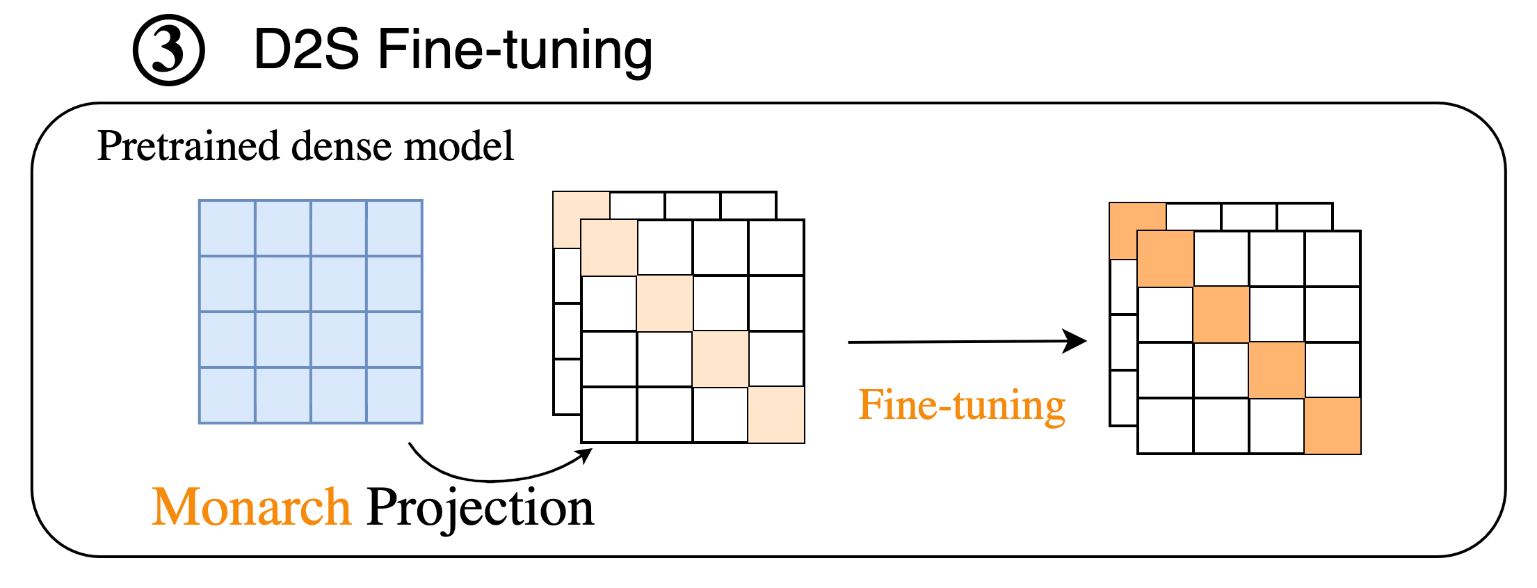
Figure 4: With Algorithm 1 for our Monarch parameterization, we can convert a pretrained model into a model with Monarch weight matrices and speed up downstream fine-tuning.

4 Using Monarch Matrices in Model Training

We can use our class of Monarch matrices to parameterize weight matrices of deep learning models in several settings.

• In the E2E sparse training setting, we replace the dense weight matrices of a baseline model with Monarch matrices with the same dimension, initialize them randomly, and train as usual. Most of our baseline models are Transformers, and we replace the projection matrices in the attention blocks, along with the weights of the feed-forward network (FFN) blocks, with Monarch matrices. The Monarch parameterization is differentiable, and we rely on autodifferentiation to train with first-order methods such as Adam [57].

• In the S2D training setting, we first replace the dense weight matrices of a baseline model with Monarch matrices, then train the sparse model for about 90% of the usual number of iterations. We then convert the Monarch matrices to dense matrices (by simply multiplying the factors $L$ and $R$ along with permutations), and continue training for the remaining 10% of the iterations. Compared to dense end-to-end training, we train for the same number of iterations, but the first 90% of the iterations are faster due to the hardware efficiency of Monarch matrices.

• In the D2S fine-tuning setting, we start with a dense pretrained model (e.g., BERT), and project the dense weight matrices (e.g., in the attention blocks and FFN blocks) on the set of Monarch matrices using the algorithm in Section 3.3. We then fine-tune the resulting model on downstream tasks (e.g., GLUE), using first-order methods.

We typically set the number of blocks in the block-diagonal matrices to be between 2 and 4 based on the parameter budgets (25% – 50% of the dense model).

5 Experiments

We validate our approach empirically, showing that our Monarch matrix parametrization achieves a favorable efficiency–accuracy tradeoff compared to baselines on a wide range of domains (text, images, PDEs, MRI), in three settings (E2E training, S2D training, and D2S fine-tuning):

• In Section 5.1.1, on image classification and language modeling benchmarks, such as ViT / MLP Mixer on ImageNet and GPT-2 on Wikitext-103, Monarch is 2$\times$ faster to train than dense models, while achieving the same accuracy / perplexity. In Section 5.1.2, in scientific and medical domains where special transforms (Fourier) are common, Monarch outperforms Fourier transform based methods on PDE solving, with up to 40% lower error, and on MRI reconstruction attains up to 15% higher pSNR and 3.8% higher SSIM.

• In Section 5.1.2, we show that on the large OpenWebText dataset, reverse sparsification (training with Monarch weight matrices for most of the time, then transitioning to dense weight matrices) speeds up the pretraining of GPT-2 models by 2$\times$ compared to the dense model, with no loss in upstream or downstream quality. Moreover, reverse sparsification speeds up BERT pretraining by 23% even compared to the implementation from Nvidia that set the MLPerf [72] 1.1 record.

• In Section 5.3, as a proof of concept, we demonstrate that our Monarch approximation algorithm can improve fine-tuning efficiency for pretrained models. We show that compressing BERT to a Monarch matrix model performs comparably to a finetuned dense model on GLUE, with 2$\times$ fewer parameters and 1.7$\times$ faster finetuning speed.

5.1 End-to-End Training

5.1.1 Benchmark Tasks: Image Classification, Language Modeling

We show that replacing dense matrices with Monarch matrices in ViT, MLP-Mixer, and GPT-2 can speed up training by up to 2$\times$ without sacrificing model quality in Tables 1 and 2.

Setup. We use the popular vision benchmark, ImageNet [17]. We choose recent popular Vision Transformer [24], and MLP-Mixer [99] as representative base dense models. For language modeling, we evaluate GPT-2 [86] on WikiText-103 [73].

Table 1: The performance of Monarch matrices and ViT / MLP-Mixer on ImageNet, including the number of parameters and FLOPs. We measure the Top-1 accuracy and the training time speedup compared to the corresponding dense model.

Model	ImageNet acc.	Speedup	Params	FLOPs
Mixer-S/16	74.0	-	18.5M	3.8G
Monarch-Mixer-S/16	73.7	1.7$\times$	7.0M	1.5G
Mixer-B/16	77.7	-	59.9M	12.6G
Monarch-Mixer-B/16	77.8	1.9$\times$	20.9M	5.0G
ViT-S/16	79.4	-	48.8M	9.9G
Monarch-ViT-S/16	79.1	1.9$\times$	19.6M	3.9G
ViT-B/16	78.5	-	86.6M	17.6G
Monarch-ViT-B/16	78.9	2.0$\times$	33.0M	5.9G

Table 2: Performance of Monarch matrices and GPT-2-Small/Medium on WikiText-103, including the # of parameters and FLOPs. Monarch achieves similar perplexity (ppl) but 2.0$\times$ faster.

Model	PPL	Speedup	Params	FLOPs
GPT-2-Small	20.6	-	124M	106G
Monarch-GPT-2-Small	20.7	1.8$\times$	72M	51G
GPT-2-Medium	20.9	-	355M	361G
Monarch-GPT-2-Medium	20.3	2.0$\times$	165M	166G

5.1.2 PDE solving and multi-coil MRI reconstruction

Many scientific or medical imaging tasks rely on specialized transforms such as the Fourier transform. We show that replacing the fixed Fourier transform with the more expressive Monarch matrices yields higher model quality (lower reconstruction error) with comparable model speed.

Solving PDEs with Monarch Neural Operators. We follow the experimental setting in FNO [65] and apply a Monarch–based neural operator to the task of solving the Navier–Stokes PDE. Compared to baseline U-Nets [90], TF-Nets [103], ResNets [47] and FNOs [65], neural operators based on Monarch improve solution accuracy across spatial resolutions by up to $40\%$ (Table 3).

Non-periodic boundary conditions.

Traditional spectral methods based on Fourier transform work best with periodic boundary conditions and forcing terms. However, PDEs of practical interest often exhibit non–periodic or even unknown boundary conditions. Monarch operators are not constrained to the Fourier transform and can thus still learn the solution operator with excellent accuracy.

Table 3: Benchmarks on Navier-Stokes (fixing resolution 64 × 64 for both training and testing). Decreasing the viscosity coefficient $\nu$ makes the dynamics more chaotic.

Model	$v=10^{-3}$	$v=10^{-4}$	$v=10^{-5}$
U-Net	0.025	0.205	0.198
TF-Net	0.023	0.225	0.227
ResNet	0.070	0.287	0.275
FNO	0.017	0.178	0.155
Monarch-NO	0.010	0.145	0.136

Accelerated MRI Reconstruction. We characterize the utility of Monarch-based FFT operations for accelerated MRI reconstruction, a task which requires methods with both structured Fourier operators and dealiasing properties to recover high quality images. On the clinically-acquired 3D MRI SKM-TEA dataset [20], Monarch-SENSE (mSENSE) enhances image quality by over 1.5dB pSNR and 2.5% SSIM compared to zero-filled SENSE and up to 4.4dB and 3.8% SSIM compared to U-Net baselines in data-limited settings. Setup details are available in Section E.5.

Expressive FFT.

By definition, standard IFFT in zero-filled SENSE cannot dealias the signal, resulting in artifacts in the reconstructed image. mSENSE replaces the inverse FFT (IFFT) operation in standard SENSE with learnable Monarch matrices. Thus, mSENSE preserves the structure of the Fourier transform while learning to reweight frequencies to suppress aliasing artifacts. Across multiple accelerations, mSENSE achieved up to +1.5dB and 2.5% improvement in peak signal-to-noise ratio (pSNR) and structural similarity (SSIM), respectively (Table 4).

Data Efficiency.

While CNNs have shown promise for MRI reconstruction tasks, training these networks requires extensive amounts of labeled data to avoid overfitting. However, large data corpora are difficult to acquire in practice. mSENSE can be trained efficiently with limited supervised examples. In few shot settings, mSENSE can outperform U-Net by +4.4dB ($\approx$15%) and 3.8% SSIM (Table 5).

Table 4: Mean $\pm$ standard error of the mean of conventional and Monarch-SENSE (mSENSE) on dual-echo (E1,E2) MRI reconstruction at multiple acceleration factors (Acc.).

		pSNR (dB) ($\uparrow$)		SSIM ($\uparrow$)
Acc.	Model	E1	E2	E1	E2
2	SENSE	32.8$\pm$0.2	35.4$\pm$0.2	0.871$\pm$0.003	0.865$\pm$0.003
	mSENSE	34.3$\pm$0.2	36.6$\pm$0.2	0.886$\pm$0.002	0.882$\pm$0.003
3	SENSE	30.9$\pm$0.2	33.5$\pm$0.2	0.819$\pm$0.004	0.795$\pm$0.004
	mSENSE	32.3$\pm$0.2	34.6$\pm$0.2	0.843$\pm$0.003	0.820$\pm$0.004
4	SENSE	30.1$\pm$0.2	32.8$\pm$0.2	0.789$\pm$0.004	0.753$\pm$0.005
	mSENSE	31.2$\pm$0.2	33.5$\pm$0.2	0.812$\pm$0.003	0.767$\pm$0.005

Table 5: Impact of number of training examples ($N$) on dual-echo MRI reconstruction at 2x acceleration.

		pSNR (dB) ($\uparrow$)		SSIM ($\uparrow$)
$N$	Model	E1	E2	E1	E2
N/A	SENSE	32.8$\pm$0.2	35.4$\pm$0.2	0.871$\pm$0.003	0.865$\pm$0.003
1	U-Net	29.4$\pm$0.2	34.4$\pm$0.3	0.848$\pm$0.004	0.857$\pm$0.004
	mSENSE	33.8$\pm$0.2	36.0$\pm$0.2	0.886$\pm$0.003	0.867$\pm$0.003
2	U-Net	29.9$\pm$0.3	35.1$\pm$0.3	0.858$\pm$0.003	0.871$\pm$0.003
	mSENSE	34.0$\pm$0.2	36.4$\pm$0.2	0.883$\pm$0.002	0.877$\pm$0.003
3	U-Net	31.0$\pm$0.3	35.2$\pm$0.3	0.866$\pm$0.003	0.867$\pm$0.004
	mSENSE	33.9$\pm$0.2	36.5$\pm$0.2	0.882$\pm$0.002	0.878$\pm$0.003
5	U-Net	31.4$\pm$0.3	35.6$\pm$0.2	0.877$\pm$0.002	0.870$\pm$0.003
	mSENSE	33.9$\pm$0.2	36.5$\pm$0.2	0.881$\pm$0.002	0.877$\pm$0.003

5.2 Sparse-to-Dense Training (reverse sparsification)

GPT-2 pretraining.

On the large OpenWebtext dataset [36], we train a GPT-2 model with Monarch weight matrices for 90% of the training iterations, then relax the constraint on the weight matrices and train them as dense matrices for the remaining 10% of the iterations. We call this technique “reverse sparsification.” Previous sparse training techniques often don’t speed up training, whereas our hardware-efficient Monarch matrices do. Therefore we can use them as an intermediate step to pretrain a large language model (GPT-2) in 2$\times$ less time. We also evaluate its downstream quality on zero-shot generation from [34] and classification tasks from [108], achieving comparable performance to the dense counterparts (Table 6).

Table 6: The performance (accuracy) of GPT-2-medium trained with Monarch reverse sparsification and with conventional dense training on text classification benchmarks.

Model	OpenWebText (ppl)	Speedup	Classification (avg acc)
GPT-2m	18.0	-	38.9
Monarch-GPT-2m	18.0	2$\times$	38.8

In Fig. 5, we show the training time of the dense GPT-2 model, along with the Monarch GPT-2 model. After training the Monarch model for 90% of the time, in the last 10% of the training steps, by transitioning to dense weight matrices, the model is able to reach the same performance of another model that was trained with dense weight matrices from scratch. By training with Monarch matrices for 90% of the time, we reduce the total training time by 2$\times$.

BERT pretraining.

On the Wikipedia + BookCorpus datasets [110], we train a BERT-large model with Monarch weight matrices for 70% of the time and transition to dense weight matrices for the remaining 30% of the time, which yields the same pretraining loss as conventional dense training. In Table 7, we compare the total training time to several baseline implementations: the widely-used implementation from HuggingFace [104], the more optimized implementation from Megatron [94], and the most optimized implementation we know of from Nvidia that was used to set MLPerf 1.1 training speed record. Our method is 3.5x faster than HuggingFace and 23% faster than Nvidia’s MLPerf 1.1 implementation. Experiment details are in Section E.4.

Table 7: The total training time of BERT-large trained with Monarch reverse sparsification and with conventional dense training on 8 A100-40GB GPUs (DGX A100). Training consists of two phases, phase 1 with sequence length 128 and phase 2 with sequence length 512. Monarch training is 3.5x faster than HuggingFace and 23% faster than Nvidia’s MLPerf 1.1 implementation.

Implementation	Training time (h)
HuggingFace	84.5
MegaTron	52.5
Nvidia MLPerf 1.1	30.2
Nvidia MLPerf 1.1 + DeepSpeed	29.3
Monarch (ours)	23.8

5.3 Dense-to-Sparse Fine-tuning

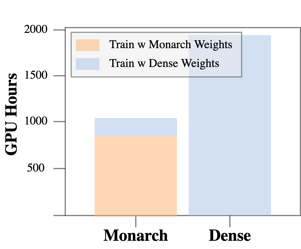
Figure 5: Time required (in A100 GPU hours) to reach the same perplexity (18.0) for GPT-2-small on OpenWebText. With “reverse sparsification”, Monarch can speed up GPT-2 training by 2$\times$.

We show that our Monarch approximation algorithm allows us to efficiently use pretrained models, such as speeding up BERT finetuning on GLUE.

BERT finetuning.

We take the BERT pretrained weights, approximate them with Monarch matrices, and finetune the resulting model on the 9 GLUE tasks. The results in Table 8 shows that we obtain a Monarch finetuned model with similar quality to the dense BERT model, but with 1.7$\times$ faster finetuning speed. This serves as a proof of concept, and we expect further speedup if additional model compression techniques are applied (e.g., quantization, kernel fusion).

Table 8: The performance of Monarch matrices in finetuning BERT on GLUE.

Model	GLUE (avg)	Speedup	Params	FLOPs
BERT-base	78.6	-	109M	11.2G
Monarch-BERT-base	78.3	1.5$\times$	55M	6.2G
BERT-large	80.4	-	335M	39.5G
Monarch-BERT-large	79.6	1.7$\times$	144M	14.6G

6 Conclusion

We propose Monarch, a novel matrix parameterization that inherits the expressiveness of butterfly matrices and thus can represent many fast transforms. Our parameterization leverages optimized batch matrix multiply routines on GPUs, yielding up to 2$\times$ speedup compared to dense matrix multiply. We derive an efficient algorithm for projecting an arbitrary dense matrix on the set of Monarch factors. Our algorithm allows us to easily fine-tune a pretrained model into a model with Monarch weight matrices. As a result, Monarch matrices unlock new ways for faster end-to-end training, sparse-to-dense training, and dense-to-sparse fine-tuning of large neural networks. By making structured matrices practical, our work is a first step towards unlocking tremendous performance improvements in applying sparse models to wide-ranging ML applications (including science and medicine). We anticipate this work can inspire more future work on advancing machine learning models for interdisciplinary research with limited computational resources.

Appendix A Extended Related Work

In this section, we extend the related works referenced in the main paper and discuss them in detail.

Sparse Training.

Our work is loosely related to neural network pruning. By iteratively eliminating neurons and connections, pruning has seen great success in compressing complex models. Han et al. [44, 45] put forth two naive but effective algorithms to compress models up to 49x and maintain comparable accuracy. Li et al. [64] employ filter pruning to reduce the cost of running convolution models up to 38 $\%$, Lin et al. [66] prunes the network at runtime, hence retaining the flexibility of the full model. Dong et al. [23] prunes the network locally in a layer by layer manner. Sanh et al. [92] prunes with deterministic first-order information, which is more adaptive to pretrained model weights. Lagunas et al. [60] prunes transformers models with block sparsity pattern during fine-tuning, which leads to real hardware speed up while maintaining the accuracy. Zhu & Gupta [109] finds large pruned sparse network consistently outperform the small dense networks with the same compute and memory footprints. Although both our and all the pruning methods are aiming to produce sparse models, we differ in our emphasis on the overall efficiency, whereas pruning mostly focuses on inference efficiency and disregards the cost in finding the smaller model.

There has been more recent work on sparse methods that focuses on speeding up training and not just inference, such as SNFS [21], RigL [21], Top-KAST [50]. These methods often focus on FLOP counts, which may not correlate well with wall-clock time on modern hardware (e.g., GPUs). Block-sparsity is another approach that exploits the block-oriented nature of GPUs [38, 7, 41]. Sparse models have also been found useful to improve the training process of dense models. For example, sparsity can be used to regularize dense models to improve accuracy [46], or to alternate between sparse and dense training to ease deployment [82]. Our sparse-to-dense reverse sparsification instead focuses on speeding up dense training, where the sparse model is used for efficiency and not regularization.

In addition, models proposed in our work can be roughly seen as a class of manually constructed lottery tickets. Lottery tickets Frankle & Carbin [30] are a set of small sub-networks derived from a larger dense network, which outperforms their parent networks in convergence speed and potentially in generalization. A huge number of studies are carried out to analyze these tickets both empirically and theoretically: Morcos et al. [75] proposed to use one generalized lottery tickets for all vision benchmarks and got comparable results with the specialized lottery tickets; Frankle et al. [31] improves the stability of the lottery tickets by iterative pruning; Frankle et al. [32] found that subnetworks reach full accuracy only if they are stable against SGD noise during training; Orseau et al. [78] provides a logarithmic upper bound for the number of parameters it takes for the optimal sub-networks to exist; Pensia et al. [81] suggests a way to construct the lottery ticket by solving the subset sum problem and it’s a proof by construction for the strong lottery ticket hypothesis. Furthermore, follow-up works [68, 102, 96] show that we can find tickets without any training labels.

Structured matrices and butterfly matrices.

Structured matrices are those with asymptotically fast matrix-vector multiplication algorithm ($o(n^{2})$ time complexity) and few parameters ($o(n^{2})$ space complexity). Common examples include sparse & low-rank matrices, and fast transforms such as Fourier transform, Chebyshev transform, Legendre transform, and more generally orthogonal polynomial transforms. These transforms have been widely used in data preprocessing (e.g., DFT in speech processing [52]) and kernel approximation [62, 106]. Many generalizations of these transforms have been used in machine learning to replace dense weight matrices [95, 98, 40]. De Sa et al. [16] shows that any structured matrix (in the form of arithmetic circuits) can be written as product of sparse matrices, and Dao et al. [13] shows that products of butterfly matrices can represent these structured matrices almost optimally in terms of runtime and memory. The class of butterfly matrices [80] have also been used in kernel models [76, 8] and deep learning models [101, 67, 1].

Neural Operators for PDEs.

Deep learning has found application in the domain of differential equations and scientific computing [85], with methods developed for prediction and control problems [56, 71], as well as acceleration of numerical schemes [83, 51]. Specific to the partial differential equations (PDEs) are approaches designed to learn solution operators [87, 29, 65], and hybridized solvers [59], evaluated primarily on classical fluid dynamics.

The promise of these approaches is to offer, at the cost of an initial training procedure, accurate yet faster solutions than an appropriate numerical method tuned for a specific problem, which can then be leveraged for real-time forecasting or within larger feedback loops. Nonetheless, optimal design of neural operators remains an open problem, with most relying on fast Fourier transforms (FFT) or standard dense neural architectures. Instead, neural operators based on Monarch are capable of approximating all fast transforms, thus allowing automated optimization towards a suitable transform on a given PDE problem.

MRI.

Accelerated multi-coil MRI is an essential mechanism for reducing long scan times and making certain scan types feasible. In multi-coil MRI, data is acquired in the spatial Fourier domain (a.k.a k-space) across multiple coils (sensors). To reduce scan time, this data is sampled below the required rate for recovering the underlying signal (i.e. Nyquist rate), which results in signal aliasing (see Appendix E.5). In these settings, direct application of the inverse fast Fourier transform (FFT) cannot suppress aliasing artifacts.

Classical MRI reconstruction approaches supplement the FFT by leveraging shared information across multiple coils and strong analytical priors to regularize image recovery objectives. SENSE-based methods jointly dealias images across multiple coils and reweight the final image based on the spatial sensitivity profile of each coil [84]. Compressed sensing promotes image sparsity in transformation domains (e.g. Fourier, wavelet) while enforcing data consistency between the Fourier transform of the reconstructed image and the observed measurements [69]. Low-rank methods enforce low rank structure across slowly-varying dimensions or local patches in the data [77, 89, 42]. Additionally, GRAPPA-based techniques optimize kernels to directly interpolate missing k-space samples to promote smoothness in the Fourier domain [39]. Despite their efficacy, these methods have long reconstruction times, require explicit analytical priors, and require careful hyperparameter fine-tuning.

CNNs have shown promise as a fast-at-inference, learnable alternative to classical MRI reconstruction methods [58]. In supervised learning, fully convolutional networks (e.g. U-Net [90] or unrolled networks [91, 43]) learn a mapping between paired zero-filled and fully-sampled, ground truth images. However, supervised methods require a large fully-sampled (labeled) data corpus and are sensitive to distribution drifts due to patient, hardware, and sequence heterogeneity [15]. To reduce dependence on labeled data, unsupervised methods have used generative adversarial networks [9, 70], self-supervised learning [105], dictionary learning [61], and untrained networks [14]. Despite their label efficiency, these techniques still underperform supervised methods and are also sensitive to distribution shift. Recently, a family of semi-supervised reconstruction methods demonstrated label efficiency and robustness to physics-driven perturbations, such as changes in signal-to-noise ratio or patient motion [19, 18]. However, these methods require large amounts of unlabeled data, which can be difficult to curate in few-shot settings. Thus, despite their success in controlled environments, prospective clinical deployment of these models has been stifled [5].

In our work, we propose a model with a single FFT-initialized factorized Monarch matrix. Such a matrix can provide the benefits of both a simple linearized transformation like FFT and a learnable mechanism to remove aliasing artifacts resulting from the undersampled k-space. The smaller learnable parameter set may reduce overfitting in data-limited settings while preserving the transformation structure of Fourier matrices. Thus, our approach can be interpreted as a hybrid between analytically-constrained classical methods and data-dependent CNNs.

Appendix B Notation Review

Throughout this paper, we use lowercase to denote scalars (e.g., $k$), lowercase boldface to denote vectors (e.g., $\mathbf{v}$), and uppercase boldface to denote matrices (e.g., $\mathbf{A}$).

$\mathbf{I}$ denotes the identity matrix. We use $\mathbf{A}^{\top}$ to denote the transpose of a matrix and $\mathbf{A}^{*}$ to denote the conjugate transpose of a matrix. All results in this paper apply to matrices over the either the reals $\mathbb{R}$ or the complex numbers $\mathbb{C}$; when the field under consideration can be either one of these, we denote it by $\mathbb{F}$.

We use 1-indexing throughout this paper except where explicitly stated.

Appendix C General Monarch Matrix Parametrization

In Section C.1, we define a parametrization for square Monarch matrices of different “block sizes” (i.e., not necessarily $\sqrt{n}$), and prove some basic properties about them. In Section C.2, we further extend this to define rectangular Monarch matrices, and prove some basic properties about them.

Note: In this section, we use 0-indexing rather than 1-indexing, for notational convenience.

C.1 General square matrices

C.1.1 Parametrization

In this section, we define a more general Monarch parametrization for square matrices, allowing for different “block sizes.” Like Definition 3.1, the parametrization involves the product of a permuted block-diagonal matrix with another block-diagonal matrix; the difference is that we now allow the matrices $\mathbf{L}$ and $\mathbf{R}$ to have diagonal blocks of different sizes. Thus, the permutations applied to $\mathbf{L}$ (to turn it into a block matrix where each block matrix is diagonal) will correspondingly also be different.

First, in Definition C.1, we define notation for a class of block-diagonal matrices.

Definition C.1 (Class $\mathcal{B}\mathcal{D}^{(b,n)}$).

Let $b\in(1,n)$ be an integer that divides $n$. For $0\leq i<\frac{n}{b}$, let $\mathbf{R}_{i}\in\mathbb{F}^{b\times b}$ be a $b\times b$ “block” matrix. Then define the matrix $\mathbf{R}$ with block size $b$ as follows:

$$\mathbf{R}=\mathrm{diag}\left(\mathbf{R}_{0},\dots,\mathbf{R}_{\frac{n}{b}-1}\right).$$ (3)

(Note that the number of possible nonzero values in $\mathbf{R}$ is $\frac{n}{b}\cdot b^{2}=nb$.) We denote the class of all matrices $\mathbf{R}$ expressible in this form by $\mathcal{B}\mathcal{D}^{(b,n)}$. Note that this class is closed under (conjugate) transposition and contains the identity matrix.

Next, in Definition C.2, we define notation for a class of block matrices whose blocks are diagonal.

Definition C.2 (Class $\mathcal{D}\mathcal{B}^{(b,n)}$).

Let $b\in(1,n)$ be an integer that divides $n$. For $0\leq i,j<b$, let $\mathbf{D}_{i,j}\in\mathbb{F}^{b\times b}$ be a $b\times b$ diagonal matrix. Then let $\mathbf{L}$ be an $n\times n$ matrix with the following form:

$$\mathbf{L}=\begin{bmatrix}\mathbf{D}_{0,0}&\dots&\mathbf{D}_{0,\frac{n}{b}-1}\\ \vdots&\ddots&\vdots\\ \mathbf{D}_{\frac{n}{b}-1,0}&\dots&\mathbf{D}_{\frac{n}{b}-1,\frac{n}{b}-1}\end{bmatrix}$$ (4)

(Note that the number of possible nonzero values in $\mathbf{L}$ is $\left({\frac{n}{b}}\right)^{2}\cdot b=\frac{n^{2}}{b}$.) We denote the class of all matrices $\mathbf{L}$ expressible in this form by $\mathcal{D}\mathcal{B}^{(b,n)}$. Note that this class is closed under (conjugate) transposition and contains the identity matrix. As we show in Section C.1.2, $\mathbf{L}$ can be written as a block-diagonal matrix with $b$ blocks of size $\tfrac{n}{b}\times\tfrac{n}{b}$ (i.e., a matrix in $\mathcal{B}\mathcal{D}^{(\frac{n}{b},\,n)}$), multiplied on the left and right with appropriate permutation matrices. We denote the class of all matrices $\mathbf{L}$ expressible in this form by $\mathcal{D}\mathcal{B}^{(b,n)}$. Note that this class is closed under (conjugate) transposition. As we show in Section C.1.2, $\mathbf{L}$ can be written as a block-diagonal matrix with $b$ blocks of size $\tfrac{n}{b}\times\tfrac{n}{b}$ (i.e., a matrix in $\mathcal{B}\mathcal{D}^{(\frac{n}{b},\,n)}$), multiplied on the left and right with appropriate permutation matrices.

Using these two definitions, we define the class of Monarch matrices with a given block size.

Definition C.3 (Class $\mathcal{M}^{(b,n)}$).

Let $b\in(1,n)$ be an integer that divides $n$. A Monarch matrix of size $n\times n$ and “block size $b$” is a matrix of the form:

$$\mathbf{M}=\mathbf{L}\mathbf{R}$$ (5)

where $\mathbf{L}\in\mathcal{D}\mathcal{B}^{(b,n)}$ and $\mathbf{R}\in\mathcal{B}\mathcal{D}^{(b,n)}$.

We denote the class of all matrices $\mathbf{M}$ expressible in this form by $\mathcal{M}^{(b,n)}$. Observe that when $b=\sqrt{n}$, this is exactly the matrix class $\mathcal{M}^{(n)}$ in Definition 3.1. (In other words, $\mathcal{M}^{(n)}$ is shorthand for $\mathcal{M}^{(\sqrt{n},n)}$.) Note that a matrix in $\mathcal{M}^{(b,n)}$ is represented by $\frac{n^{2}}{b}+nb$ parameters.

We remark that $\mathcal{M}^{(b,n)}\supset\mathcal{B}^{(n)}$ for all block sizes $b\in(1,n)$ that divide $n$.

Based on Definition C.19, we define the classes $\mathcal{M}\mathcal{M}^{*(b,n)}$ and $\mathcal{M}^{*}\mathcal{M}^{(b,n)}$::

Definition C.4 (Class $\mathcal{M}\mathcal{M}^{*(b,n)}$, $\mathcal{M}^{*}\mathcal{M}^{(b,n)}$).

Let $b\in(1,n)$ be an integer that divides $n$ and suppose $\mathbf{M}_{1},\mathbf{M}_{2}\in\mathcal{M}^{(b,n)}$. We define $\mathcal{M}\mathcal{M}^{*(b,n)}$ to be the the class of all matrices $\mathbf{M}$ expressible in the form $\mathbf{M}=\mathbf{M}_{1}\mathbf{M}_{2}^{*}$.
We define $\mathcal{M}^{*}\mathcal{M}^{(b,n)}$ to be the the class of all matrices $\mathbf{M}$ expressible in the form $\mathbf{M}=\mathbf{M}_{1}^{*}\mathbf{M}_{2}$.

Observe that when $b=\sqrt{n}$, $\mathcal{M}\mathcal{M}^{*(b,n)}$ is exactly the matrix class $\mathcal{M}\mathcal{M}^{*(n)}$ defined in Section 3. Note that a matrix in $\mathcal{M}\mathcal{M}^{*(b,n)}$ or $\mathcal{M}^{*}\mathcal{M}^{(b,n)}$. is represented by $2\frac{n^{2}}{b}+2nb$ parameters.

Finally, we define the following “Monarch hierarchy” based on the kaleidoscope hierarchy of [13]:

Definition C.5 (Class $(\mathcal{M}\mathcal{M}^{*(b,n)})^{w}_{e}$).

Let $b\in(1,n)$ be an integer that divides $n$. We define the matrix class $(\mathcal{M}\mathcal{M}^{*(b,n)})^{w}_{e}$ as the set of all matrices $\mathbf{M}$ that can be expressed as

$$\mathbf{M}=\left({\prod\limits_{i=1}^{w}}\mathbf{M}_{i}\right)[1:n,1:n]$$ (6)

where each $\mathbf{M}_{i}\in\mathcal{M}\mathcal{M}^{*(b,e\cdot n)}$.

Note that a matrix in $(\mathcal{M}\mathcal{M}^{*(b,n)})^{w}_{e}$ is represented by $2w\frac{e^{2}n^{2}}{b}+2wenb$ parameters.

C.1.2 Properties

Here we show some properties of the matrix classes defined above. We first show some basic equivalent ways to define these classes. We then show (Theorem 3) that the matrices in $\mathcal{D}\mathcal{B}^{(b,n)}$ are permuted block-diagonal matrices; specifically, that they can be converted to matrices in $\mathcal{B}\mathcal{D}^{(\frac{n}{b},n)}$ by applying the appropriate permutation. Finally, we state an expressivity result for the general “Monarch hierarchy” which follows from Theorem 1 of [13].

First, we define a class of permutations. Let $1\leq b\leq n$ be integers such that $b$ divides $n$. We will need to express each index $0\leq i<n$ in “block form.” More specifically:

Definition C.6.

Let $i\geq 0$, $b\geq 1$ be integers. Then define

$$i_{0}=i\text{ mod }{b},$$

and

$$i_{1}=\left\lfloor\frac{i}{b}\right\rfloor.$$

We use the notation $i\equiv\left({{i_{1}},{i_{0}}}\right)_{{b}}$ to denote the representation above. In particular, if $i\equiv(i_{1},i_{0})_{b}$, then we have

$$i=i_{1}\cdot b+i_{0}$$

Using this notation, we define the following class of permutations:

Definition C.7.

Let $b\in[1,n]$ be an integer that divides $n$. Let $i\equiv\left({{i_{1}},{i_{0}}}\right)_{{b}}$. Define

$$\sigma_{(b,n)}(i)=i_{0}\cdot\frac{n}{b}+i_{1}.$$ (7)

That is, $\sigma_{(b,n)}(i)\equiv\left({{i_{0}},{i_{1}}}\right)_{{\frac{n}{b}}}$. Let $\mathbf{P}_{(b,n)}$ denote the $n\times n$ permutation matrix defined by the permutation $\sigma_{(b,n)}$.

Intuitively, $\mathbf{P}_{(b,n)}$ can be interpreted as reshaping a length-$n$ vector into an $b\times\tfrac{n}{b}$ matrix in row-major order, transposing the result, and then flattening this back into a vector (again in row-major order).

Now, we restate the formulation in Definition C.1 equivalently as:

Proposition C.8.

A matrix $\mathbf{R}$ satisfies Equation 3 (i.e., $\mathbf{R}\in\mathcal{B}\mathcal{D}^{(b,n)}$) if and only if the following holds for any $0\leq i,j<n$. Let $i\equiv\left({{i_{1}},{i_{0}}}\right)_{{b}}$ and $j\equiv\left({{j_{1}},{j_{0}}}\right)_{{b}}$. Then

1. if $i_{1}\neq j_{1}$, then $\mathbf{R}[i,j]=0$.

2. Else (i.e., when $i_{1}=j_{1}$), then $\mathbf{R}[i,j]=\mathbf{R}_{i_{1}}[i_{0},j_{0}]$.

We restate the formulation in Definition C.2 equivalently as:

Proposition C.9.

A matrix $\mathbf{L}$ satisfies Equation 4 (i.e., $\mathbf{L}\in\mathcal{D}\mathcal{B}^{(b,n)}$) if and only if the following holds for any $0\leq i,j<n$. Let $i\equiv\left({{i_{1}},{i_{0}}}\right)_{{b}}$ and $j\equiv\left({{j_{1}},{j_{0}}}\right)_{{b}}$. Then

1. if $i_{0}\neq j_{0}$, then $\mathbf{L}[i,j]=0$.

2. Else, (i.e., when $i_{0}=j_{0}$), then $\mathbf{L}[i,j]=\mathbf{D}_{i_{1},j_{1}}[i_{0},i_{0}]$.

We will argue the following:

Theorem 3.

Let $1\leq b\leq n$ such that $b$ divides $n$. Recall that $\mathbf{P}_{(b,n)}$ is the permutation matrix defined by the permutation $\sigma_{(b,n)}$. Let $\mathbf{L}$ be a matrix in $\mathcal{D}\mathcal{B}^{(b,n)}$. Then we have

$$\mathbf{R}^{\prime}=\mathbf{P}_{(b,n)}\cdot\mathbf{L}\cdot\mathbf{P}_{(b,n)}^{\top},$$

where $\mathbf{R}^{\prime}\in\mathcal{B}\mathcal{D}^{(\frac{n}{b},\,n)}$.

Proof.

We first note that multiplying an $n\times n$ matrix on the right (and left resp.) by $\mathbf{P}_{(b,n)}^{\top}=\mathbf{P}_{(\frac{n}{b},n)}$ (and $\mathbf{P}_{(b,n)}$ resp.) permutes the columns (and rows resp.) of the matrix according to $\sigma_{(b,n)}$. This implies that for any $0\leq i,j<n$:

$$\mathbf{R}^{\prime}[\sigma_{(b,n)}(i),\sigma_{(b,n)}(j)]=\mathbf{L}[i,j].$$ (8)

To complete the proof, we will argue that $\mathbf{R}^{\prime}$ satisfies the two conditions in Proposition C.8.

Towards this end, let $0\leq i,j<n$ be arbitrary indices and further, define $i=\left({{i_{1}},{i_{0}}}\right)_{{b}}$ and $j=\left({{j_{1}},{j_{0}}}\right)_{{b}}$. Then note that $\sigma_{(b,n)}(i)=\left({{i_{0}},{i_{1}}}\right)_{{\frac{n}{b}}}$ and $\sigma_{(b,n)}(j)=\left({{j_{0}},{j_{1}}}\right)_{{\frac{n}{b}}}$.

By Proposition C.9, we have that if $i_{0}\neq j_{0}$, then $\mathbf{L}[i,j]=0$. Note that $i_{0}\neq j_{0}$ satisfies the pre-condition for base size $\frac{n}{b}$ for indices $(\sigma_{(b,n)}(i),\sigma_{(b,n)}(j))$ in item 1 in Proposition C.8. Then by Eq. 8, we have that $\mathbf{R}^{\prime}[\sigma_{(b,n)}(i),\sigma_{(b,n)}(j)]=0$, which satisfies item 1 in Proposition C.8.

Now consider the case that $i_{0}=j_{0}$; then by item 2 in Proposition C.9, we have that $\mathbf{L}[i,j]=\mathbf{D}_{i_{1},j_{1}}[i_{0},i_{0}]$. Note that $i_{0}=j_{0}$ satisfies the pre-condition for base size $\frac{n}{b}$ for indices $(\sigma_{(b,n)}(i),\sigma_{(b,n)}(j))$ in item 2 in Proposition C.8 if we define $\mathbf{R}^{\prime}_{i_{0}}\in\mathbb{F}^{\frac{n}{b}\times\frac{n}{b}}$ as follows:

$$\mathbf{R}^{\prime}_{i_{0}}[i_{1},j_{1}]=\mathbf{D}_{i_{1},j_{1}}[i_{0},i_{0}].$$

Note that the above implies that

$$\mathbf{R}^{\prime}=\mathrm{diag}\left({\mathbf{R}^{\prime}_{0},\dots,\mathbf{R}^{\prime}_{b-1}}\right),$$

where $\mathbf{R}^{\prime}_{\cdot}$ is as defined in the above paragraph. This means $\mathbf{R}^{\prime}\in\mathcal{B}\mathcal{D}^{(\frac{n}{b},n)}$, since each block $\mathbf{R}_{i_{0}}^{\prime}$ is a matrix of size $\frac{n}{b}\times\frac{n}{b}$. ∎

We now briefly note some alternate ways to express matrices in $\mathcal{M}\mathcal{M}^{*(b,n)}$.

Proposition C.10.

For any $\mathbf{M}\in\mathcal{M}\mathcal{M}^{*(b,n)}$, we can write $\mathbf{M}=(\mathbf{P}_{(b,n)}^{\top}\mathbf{L}_{1}\mathbf{P}_{(b,n)})\mathbf{R}(\mathbf{P}_{(b,n)}^{\top}\mathbf{L}_{2}\mathbf{P}_{(b,n)})$, where $\mathbf{L}_{1},\mathbf{L}_{2}\in\mathcal{B}\mathcal{D}^{(\frac{n}{b},n)}$ and $\mathbf{R}\in\mathcal{B}\mathcal{D}^{(b,n)}$.

Proof.

By definition (see Definition C.1 and Definition C.2), if $\mathbf{M}\in\mathcal{M}\mathcal{M}^{*(b,n)}$, we can write $\mathbf{M}=(\mathbf{L}_{1}^{\prime}\mathbf{R}_{1})(\mathbf{L}_{2}^{\prime}\mathbf{R}_{2})^{*}=\mathbf{L}_{1}^{\prime}(\mathbf{R}_{1}^{*}\mathbf{R}_{2})\mathbf{L}_{2}^{\prime*}$, where $\mathbf{L}_{1}^{\prime},\mathbf{L}_{2}^{\prime}\in\mathcal{D}\mathcal{B}^{(b,n)},\mathbf{R}_{1},\mathbf{R}_{2}\in\mathcal{B}\mathcal{D}^{(b,n)}$.

Notice that since $\mathbf{R}_{1}^{*},\mathbf{R}_{2}$ are both block-diagonal with the same structure (i.e., both have blocks of size $b\times b$), their product $\mathbf{R}$ is also in $\mathcal{B}\mathcal{D}^{(b,n)}$. Also, by Theorem 3 we can write $\mathbf{L}_{1}=\mathbf{P}_{(b,n)}\mathbf{L}_{1}^{\prime}\mathbf{P}_{(b,n)}^{\top}$, $\mathbf{L}_{2}=\mathbf{P}_{(b,n)}\mathbf{L}_{2}^{\prime}\mathbf{P}_{(b,n)}^{\top}$, where $\mathbf{L}_{1},\mathbf{L}_{2}$ are both in $\mathcal{B}\mathcal{D}^{(\frac{n}{b},n)}$ (i.e., block diagonal with blocks of size $\frac{n}{b}\times\frac{n}{b}$).

Thus, we can write $\mathbf{M}=(\mathbf{P}_{(b,n)}^{\top}\mathbf{L}_{1}\mathbf{P}_{(b,n)})\mathbf{R}(\mathbf{P}_{(b,n)}^{\top}\mathbf{L}_{2}\mathbf{P}_{(b,n)})$, where $\mathbf{L}_{1},\mathbf{L}_{2}\in\mathcal{B}\mathcal{D}^{(\frac{n}{b},n)}$ and $\mathbf{R}\in\mathcal{B}\mathcal{D}^{(b,n)}$. ∎

We use the above to show a simple relationship between $\mathcal{M}\mathcal{M}^{*(b,n)}$ and $\mathcal{M}^{*}\mathcal{M}^{(b,n)}$.

Proposition C.11.

If $\mathbf{M}\in\mathcal{M}\mathcal{M}^{*(b,n)}$, then $\mathbf{P}_{(b,n)}\mathbf{M}\mathbf{P}_{(b,n)}^{\top}\in\mathcal{M}^{*}\mathcal{M}^{(\frac{n}{b},n)}$. Conversely, if $\mathbf{M}\in\mathcal{M}^{*}\mathcal{M}^{(b,n)}$, then $\mathbf{P}_{(b,n)}^{\top}\mathbf{M}\mathbf{P}_{(b,n)}\in\mathcal{M}^{*}\mathcal{M}^{(\frac{n}{b},n)}$.

Proof.

Suppose $\mathbf{M}\in\mathcal{M}\mathcal{M}^{*(b,n)}$. By Proposition C.10 we can write $\mathbf{M}=(\mathbf{P}_{(b,n)}^{\top}\mathbf{L}_{1}\mathbf{P}_{(b,n)})\mathbf{R}(\mathbf{P}_{(b,n)}^{\top}\mathbf{L}_{2}\mathbf{P}_{(b,n)})$, where $\mathbf{L}_{1},\mathbf{L}_{2}\in\mathcal{B}\mathcal{D}^{(\frac{n}{b},n)}$ and $\mathbf{R}\in\mathcal{B}\mathcal{D}^{(b,n)}$. Thus $\mathbf{P}_{(b,n)}\mathbf{M}\mathbf{P}_{(b,n)}^{\top}=\mathbf{L}_{1}(\mathbf{P}_{(b,n)}\mathbf{R}\mathbf{P}_{(b,n)}^{\top})\mathbf{L}_{2}$.

Letting $\mathbf{L}_{1}^{\prime}=\mathbf{L}_{1},\mathbf{L}_{2}^{\prime}=\mathbf{L}_{2}^{*},\mathbf{R}_{1}^{\prime}=\mathbf{P}_{(b,n)}\mathbf{R}\mathbf{P}_{(b,n)}^{\top}$, and $\mathbf{R}_{2}^{\prime}=\mathbf{I}$, we have $\mathbf{L}_{1}^{\prime},\mathbf{L}_{2}^{\prime}\in\mathcal{B}\mathcal{D}^{(\frac{n}{b},n)}$, $\mathbf{R}_{1}^{\prime},\mathbf{R}_{2}^{\prime}\in\mathcal{D}\mathcal{B}^{(\frac{n}{b},n)}$, and $\mathbf{L}_{1}(\mathbf{P}_{(b,n)}\mathbf{R}\mathbf{P}_{(b,n)}^{\top})\mathbf{L}_{2}=\mathbf{L}_{1}^{\prime}\mathbf{R}_{1}^{\prime}\mathbf{R}_{2}^{\prime*}\mathbf{L}_{2}^{\prime*}=(\mathbf{L}_{1}^{\prime}\mathbf{R}_{1}^{\prime})(\mathbf{L}_{2}^{\prime}\mathbf{R}_{2}^{\prime})^{*}=\mathbf{M}_{1}^{\prime}\mathbf{M}_{2}^{\prime*}$, where $\mathbf{M}_{1}^{\prime}=\mathbf{L}_{1}^{\prime}\mathbf{R}_{1}^{\prime},\mathbf{M}_{2}^{\prime}=\mathbf{L}_{2}^{\prime}\mathbf{R}_{2}^{\prime}$, so $\mathbf{M}_{1}^{\prime},\mathbf{M}_{2}^{\prime}\in\mathcal{M}^{*}\mathcal{M}^{(\frac{n}{b},n)}$.

Now instead suppose $\mathbf{M}\in\mathcal{M}^{*}\mathcal{M}^{(b,n)}$. So $\mathbf{M}=\mathbf{M}_{1}^{*}\mathbf{M}_{2}=\mathbf{R}_{1}^{*}\mathbf{L}_{1}^{*}\mathbf{L}_{2}\mathbf{R}_{2}$ for some $\mathbf{R}_{1},\mathbf{R}_{2}\in\mathcal{B}\mathcal{D}^{(b,n)}$ and $\mathbf{L}_{1},\mathbf{L}_{2}\in\mathcal{D}\mathcal{B}^{(b,n)}$. Thus by Theorem 3 (and the fact that $\mathcal{B}\mathcal{D}^{(b,n)}$ is closed under conjugate transposition) we can write $\mathbf{R}_{1}^{*}=\mathbf{P}_{(\frac{n}{b},n)}^{\top}\mathbf{R}_{1}^{\prime}\mathbf{P}_{(\frac{n}{b},n)}=\mathbf{P}_{(b,n)}\mathbf{R}_{1}^{\prime}\mathbf{P}_{(b,n)}^{\top}$ for some $\mathbf{R}_{1}^{\prime}\in\mathcal{D}\mathcal{B}^{(\frac{n}{b},n)}$, and similarly, can write $\mathbf{R}_{2}=\mathbf{P}_{(b,n)}\mathbf{R}_{2}^{\prime}\mathbf{P}_{(b,n)}^{\top}$ for some $\mathbf{R}_{2}^{\prime}\in\mathcal{D}\mathcal{B}^{(\frac{n}{b},n)}$.

So $\mathbf{P}_{(b,n)}^{\top}\mathbf{M}\mathbf{P}_{(b,n)}=\mathbf{R}_{1}^{\prime}(\mathbf{P}_{(b,n)})^{\top}\mathbf{L}_{1}^{*})(\mathbf{L}_{2}\mathbf{P}_{(b,n)}))\mathbf{R}_{2}^{\prime}=\mathbf{R}_{1}^{\prime}(\mathbf{P}_{(b,n)}^{\top}\mathbf{L}_{1}^{*}\mathbf{P}_{(b,n)})(\mathbf{P}_{(b,n)}^{\top}\mathbf{L}_{2}\mathbf{P}_{(b,n)})\mathbf{R}_{2}^{\prime}=(\mathbf{R}_{1}^{\prime}\mathbf{L}_{1}^{\prime})(\mathbf{L}_{2}^{\prime}\mathbf{R}_{2}^{\prime})$, where $\mathbf{L}_{1}^{\prime}=\mathbf{P}_{(b,n)}^{\top}\mathbf{L}_{1}^{*}\mathbf{P}_{(b,n)}$, $\mathbf{L}_{2}^{\prime}=\mathbf{P}_{(b,n)}^{\top}\mathbf{L}_{2}\mathbf{P}_{(b,n)}$ are in $\mathcal{B}\mathcal{D}^{(\frac{n}{b},n)}$ by Theorem 3. Thus letting $\mathbf{M}_{1}^{\prime}=\mathbf{R}_{1}^{\prime}\mathbf{L}_{1}^{\prime}$, $\mathbf{M}_{2}^{\prime}=\mathbf{R}_{2}^{*}\mathbf{L}_{2}^{\prime*}$, we have $\mathbf{M}=\mathbf{M}_{1}^{\prime}\mathbf{M}_{2}^{\prime*}$ with $\mathbf{M}_{1}^{\prime},\mathbf{M}_{2}^{\prime}\in\mathcal{M}^{*(\frac{n}{b},n)}$. ∎

We now show that the class $\mathcal{M}^{(b,n)}$ strictly contains the class $\mathcal{B}^{(n)}$ of $n\times n$ butterfly matrices (as defined in Dao et al. [13]). We first show two elementary “helper” results.

Proposition C.12.

If $b,\,c\in(1,n)$ are such that $b$ divides $c$ and $c$ divides $n$, then $\mathcal{B}\mathcal{D}^{(b,n)}\subseteq\mathcal{B}\mathcal{D}^{(c,n)}$.

Proof.

Suppose $\mathbf{R}\in\mathcal{B}\mathcal{D}^{(b,n)}$. Then by Proposition C.8, $\mathbf{R}[i,j]=0$ whenever $\left\lfloor\frac{i}{b}\right\rfloor\neq\left\lfloor\frac{j}{b}\right\rfloor$. Thus, whenever $\left\lfloor\frac{i}{c}\right\rfloor\neq\left\lfloor\frac{j}{c}\right\rfloor$, $\mathbf{R}[i,j]=0$, since $\left\lfloor\frac{i}{c}\right\rfloor\neq\left\lfloor\frac{j}{c}\right\rfloor$ implies $\left\lfloor\frac{i}{b}\right\rfloor\neq\left\lfloor\frac{j}{b}\right\rfloor$ by the assumption that $b$ divides $c$. Applying Proposition C.8 again, this means $\mathbf{R}\in\mathcal{B}\mathcal{D}^{(c,n)}$ as well. ∎

Proposition C.13.

If $b,\,c\in(1,n)$ are such that $b$ divides $c$ and $c$ divides $n$, then $\mathcal{D}\mathcal{B}^{(c,n)}\subseteq\mathcal{D}\mathcal{B}^{(b,n)}$.

Proof.

Suppose $\mathbf{L}\in\mathcal{D}\mathcal{B}^{(c,n)}$. Then by Proposition C.9, $\mathbf{L}[i,j]=0$ whenever $(i\text{ mod }c)\neq(j\text{ mod }c)$. Thus, whenever $(i\text{ mod }b)\neq(j\text{ mod }b)$, $\mathbf{L}[i,j]=0$, since $(i\text{ mod }b)\neq(j\text{ mod }b)$ implies $(i\text{ mod }c)\neq(j\text{ mod }c)$ by the assumption that $b$ divides $c$. Applying Proposition C.9 again, this means $\mathbf{L}\in\mathcal{D}\mathcal{B}^{(b,n)}$ as well. ∎

Theorem 4.

Let $n\geq 4$ be a power of 2. The class of matrices $\mathcal{B}^{(n)}$ is a subset of the class $\mathcal{M}^{(b,n)}$, for all $b\in(1,n)$ that divide $n$. When $n\geq 512$ it is a strict subset.

Proof.

Recall from Section 2.2 that if $\mathbf{B}\in\mathcal{B}^{(n)}$, it has a butterfly factorization $\mathbf{B}=\mathbf{B}_{n}\mathbf{B}_{n/2}\ldots\mathbf{B}_{2}$, where each $\mathbf{B}_{i}\in\mathcal{B}\mathcal{F}^{(n,i)}$.

Consider multiplying together the factors $\mathbf{B}_{b}\mathbf{B}_{b/2}\dots\mathbf{B}_{2}$ (where $b\in(1,n)$ divides $n$). Since $\mathbf{B}_{i}\in\mathcal{B}\mathcal{F}^{(n,i)}$, by definition it is block diagonal with diagonal blocks of size $i\times i$; in other words, $\mathbf{B}_{i}\in\mathcal{B}\mathcal{D}^{(i,n)}$. Thus, each of the matrices $\mathbf{B}_{b},\mathbf{B}_{b/2},\dots,\mathbf{B}_{2}$ is in $\mathcal{B}\mathcal{D}^{(b,n)}$ (by Proposition C.12), i.e. block-diagonal with block size $b\times b$. This means their product $\mathbf{B}_{b}\mathbf{B}_{b/2}\dots\mathbf{B}_{2}$ is also block diagonal with block size $b\times b$, i.e., it is in $\mathcal{B}\mathcal{D}^{(b,n)}$.

Now, note that since $\mathbf{B}_{i}\in\mathcal{B}\mathcal{F}^{(n,i)}$, by definition it is a block matrix with blocks of size $i/2\times i/2$, where each block is a diagonal matrix (note that some of these blocks are zero, except for the case of $\mathbf{B}_{n}$). In other words, $\mathbf{B}_{i}\in\mathcal{D}\mathcal{B}^{(i/2,n)}$. Thus, for all $i\in\{n,n/2,\dots,2b\}$, $\mathbf{B}_{i}\in\mathcal{D}\mathcal{B}^{((2b)/2,n)}=\mathcal{D}\mathcal{B}^{(b,n)}$ (by Proposition C.13). So, their product $\mathbf{B}_{n}\mathbf{B}_{n/2}\dots\mathbf{B}_{2b}$ is in $\mathcal{D}\mathcal{B}^{(b,n)}$ as well, as by Theorem 3 we can write $\mathbf{B}_{n}\mathbf{B}_{n/2}\dots\mathbf{B}_{2b}=\mathbf{P}_{(b,n)}^{\top}(\mathbf{P}_{(b,n)}\mathbf{B}_{n}\mathbf{P}_{(b,n)}^{\top})(\mathbf{P}_{(b,n)}\mathbf{B}_{n/2}\mathbf{P}_{(b,n)}^{\top})\dots(\mathbf{P}_{(b,n)}\mathbf{B}_{2b}\mathbf{P}_{(b,n)}^{\top})\mathbf{P}_{(b,n)}$ and each of the $\mathbf{P}_{(b,n)}\mathbf{B}_{i}\mathbf{P}_{(b,n)}^{\top}$’s in the preceding expression is in $\mathcal{B}\mathcal{D}^{(\frac{n}{b},n)}$.

Thus, if we let $\mathbf{L}=\mathbf{B}_{n}\mathbf{B}_{n/2}\dots\mathbf{B}_{2b}$ and $\mathbf{R}=\mathbf{B}_{b}\mathbf{B}_{b/2}\dots\mathbf{B}_{2}$, we have $\mathbf{B}=\mathbf{L}\mathbf{R}$ and $\mathbf{L}\in\mathcal{D}\mathcal{B}^{(b,n)}$, $\mathbf{R}\in\mathcal{B}\mathcal{D}^{(b,n)}$, which means that $\mathbf{B}\in\mathcal{M}^{(b,n)}$ (Definition C.19).

To show that the inclusion is strict, notice that any $\mathbf{M}\in\mathcal{M}^{(b,n)}$ is the product of $\mathbf{L}$ and $\mathbf{R}$, where $\mathbf{R}\in\mathcal{B}\mathcal{D}^{(b,n)}$ and $\mathbf{P}_{(b,n)}^{\top}\mathbf{L}\mathbf{P}_{(b,n)}\in\mathcal{B}\mathcal{D}^{(\frac{n}{b},n)}$ (by Theorem 3). Notice that the identity matrix is contained in both $\mathcal{B}\mathcal{D}^{(b,n)}$ and $\mathcal{D}\mathcal{B}^{(b,n)}$. Suppose first that $b\leq\sqrt{n}$. Then even if we set $\mathbf{R}$ to the identity, $\mathbf{M}$ has at least $\frac{n^{2}}{b}\geq n^{3/2}$ free parameters (the entries in the blocks of the block-diagonal matrix $\mathbf{P}_{(b,n)}^{\top}\mathbf{L}\mathbf{P}_{(b,n)}$ can be arbitrary, and there are $b$ such blocks each of size $\frac{n}{b}$). Similarly, in the case $b>\sqrt{n}$, we can set $\mathbf{L}$ to the identity, and $\mathbf{M}$ has at least $nb\geq n^{3/2}$ free parameters (the entries of the block-diagonal matrix $\mathbf{R}$ can be arbitrary, and there are $nb$ total of these). Thus, at least $n^{3/2}$ parameters are required to uniquely describe any matrix in $\mathcal{M}^{(b,n)}$. However, a butterfly matrix in $\mathcal{B}^{(n)}$ has only $2n\log_{2}n$ parameters. For $n>256$, $2n\log_{2}n<n^{3/2}$. (Note that this analysis is not tight: a more careful analysis can show the inclusion is strict even for smaller values of $n$.)

∎

We end this section with a theorem on the expressivity of the “monarch hierarchy” (products of monarch matrices), which follows from Theorem 1 of [13].

Theorem 5 (Monarch hierarchy expressivity).

Let $\mathbf{M}$ be an $n\times n$ matrix such that matrix-vector multiplication of $\mathbf{M}$ and an arbitrary vector $\mathbf{v}$ (i.e., computation of $\mathbf{M}\mathbf{v}$) can be represented as a linear arithmetic circuit with depth $d$ and $s$ total gates. Let $b\in(1,n)$ be a power of 2 that divides $n$. Then, $\mathbf{M}\in(\mathcal{M}\mathcal{M}^{*(b,n)})^{O(d)}_{O(s/n)}$.

Proof.

Theorem 1 of Dao et al. [13] says that if $n$ is a power of 2 and $\mathbf{A}$ is an $n\times n$ matrix such that multiplying any vector $v$ by $\mathbf{A}$ can be represented as a linear arithmetic circuit with depth $\leq d$ and $\leq s$ total gates, then $\mathbf{A}\in(\mathcal{B}\mathcal{B}^{*(n)})^{O(d)}_{O(s/n)}$ (this is the “kaleidoscope representation” of $\mathbf{A}$).

Recall from Theorem 4 that for any $b\in(1,n)$ that is a power of 2 and divides $n$, $\mathcal{M}^{(b,n)}\supset\mathcal{B}^{(n)}$; thus, this implies $\mathcal{M}\mathcal{M}^{*(b,e\cdot n)}\supset\mathcal{B}\mathcal{B}^{*(e\cdot n)}$, and in turn $(\mathcal{M}\mathcal{M}^{*(b,n)})^{w}_{e}\supset(\mathcal{B}\mathcal{B}^{*(n)})^{w}_{e}$.

As $\mathbf{A}\in(\mathcal{B}\mathcal{B}^{*(n)})^{O(d)}_{O(s/n)}$, we thus have $\mathbf{A}\in(\mathcal{M}\mathcal{M}^{*(b,n)})^{O(d)}_{O(s/n)}$. ∎

As per [13], the class of kaleidoscope matrices $(\mathcal{B}\mathcal{B}^{*(n)})^{O(d)}_{O(s/n)}$ has $O(ds\log s)$ parameters and runtime, compared to the $O(s)$ parameters and runtime of the circuit. Note that at worst, $s$ is $O(n^{2})$.

Define $f(n,s)$ to be the largest power of 2 that is $\leq\min\left\{\tfrac{n}{2},\sqrt{s}\right\}$. Note that $f(n,s)=O(\sqrt{s})$, and since $s=O(n^{2})$, $f(n,s)=\Omega(\sqrt{s})$, so $f(n,s)=\Theta(\sqrt{s})$. We thus have $\mathbf{A}\in(\mathcal{M}\mathcal{M}^{*(f(n,s),n)})^{O(d)}_{O(s/n)}$. The class $(\mathcal{M}\mathcal{M}^{*(f(n,s),n)})^{O(d)}_{O(s/n)}$ has $O(d\frac{s^{2}}{f(n,s)}+dsf(n,s))=O(ds^{3/2})$ parameters. Thus, the monarch representation of $\mathbf{A}$ is suboptimal by at most an $O(d\sqrt{s})$ factor compared to the $O(d{}\,\log s)$ of kaleidoscope.

C.2 General rectangular matrices

In this section, we extend the Monarch parametrization to apply to rectangular matrices, and prove some basic properties of the relevant matrix classes. (Note that our subsequent theoretical results (Appendix D) do not depend on this section, as they focus on the square parametrization.)

For the rest of the section, we will assume that $n_{1},n_{2},n_{3},b_{1},b_{2},b_{3}\geq 1$ are integers such that:

• $b_{i}$ divides $n_{i}$ for all $1\leq i\leq 3$, and

• $\frac{n_{1}}{b_{1}}=\frac{n_{2}}{b_{2}}$.

We begin with the definition of the following class of rectangular block-diagonal matrices:

Definition C.14.

For $0\leq i<\frac{n}{b_{1}}$, let $\mathbf{R}_{i}\in\mathbb{F}^{b_{2}\times b_{1}}$ be a $b_{2}\times b_{1}$ matrix. Then define the matrix $\mathbf{R}\in\mathbb{F}^{n_{2}\times n_{1}}$ as follows:

$$\mathbf{R}=\mathrm{diag}\left(\mathbf{R}_{0},\dots,\mathbf{R}_{\frac{n_{1}}{b_{1}}-1}\right).$$ (9)

We say that $\mathbf{R}$ has block size $b_{2}\times b_{1}$. Recall that we have assumed $\frac{n_{1}}{b_{1}}=\frac{n_{2}}{b_{2}}$, so Eq. 9 is well-defined. (Note that the number of possible nonzero values in $\mathbf{R}$ is $\frac{n_{1}}{b_{1}}\cdot b_{1}\times b_{2}=n_{1}b_{2}$.) We denote the class of all matrices $\mathbf{R}$ expressible in this form by $\mathcal{B}\mathcal{D}^{(b_{2}\times b_{1},n_{2}\times n_{1})}$. Note that this class is only defined when $\frac{n_{1}}{b_{1}}=\frac{n_{2}}{n_{2}}$.

We restate the above definition equivalently as:

Proposition C.15.

$\mathbf{R}\in\mathbb{F}^{n_{2}\times n_{1}}$ is in $\mathcal{B}\mathcal{D}^{(b_{2}\times b_{1},n_{2}\times n_{1})}$ (with $\frac{n_{1}}{b_{1}}=\frac{n_{2}}{n_{2}}$) if and only if the following holds for any $0\leq i<n_{2}$ and $0\leq j<n_{1}$. Let $i\equiv\left({{i_{1}},{i_{0}}}\right)_{{b_{2}}}$ and $j\equiv\left({{j_{1}},{j_{0}}}\right)_{{b_{1}}}$ (recalling this notation from Definition C.6. Then

1. if $i_{1}\neq j_{1}$, then $\mathbf{R}[i,j]=0$.

2. Else (i.e., when $i_{1}=j_{1}$), then $\mathbf{R}[i,j]=\mathbf{R}_{i_{1}}[i_{0},j_{0}]$.

Before we define the rectangular $\mathbf{L}$, we first need to define the notion of a ‘wrapped diagonal’ matrix:

Definition C.16.

A wrapped diagonal matrix $\mathbf{S}\in\mathbb{F}^{b_{3}\times b_{2}}$ is defined as follows. First assume $b_{2}\leq b_{3}$. Then for any $0\leq i<b_{3}$ and $0\leq j<b_{2}$, we have the following. If $i\text{ mod }{b_{2}}\neq j$, then $\mathbf{S}[i,j]=0$. (If $b_{2}>b_{3}$, then instead apply the previous definition to $\mathbf{S}^{\top}$.)

We now define the following class of block matrices with each block a wrapped diagonal matrix.

Definition C.17.

Let $\mathbf{L}\in\mathbb{F}^{n_{3}\times n_{2}}$ have the form:

$$\mathbf{L}=\begin{bmatrix}\mathbf{S}_{0,0}&\dots&\mathbf{S}_{0,\frac{n_{2}}{b_{2}}-1}\\ \vdots&\ddots&\vdots\\ \mathbf{S}_{\frac{n_{3}}{b_{3}}-1,0}&\dots&\mathbf{S}_{\frac{n_{3}}{b_{3}}-1,\frac{n_{2}}{b_{2}}-1}\end{bmatrix},$$ (10)

where each $\mathbf{S}_{\cdot,\cdot}$ is a wrapped diagonal matrix in $\mathbb{F}^{b_{3}\times b_{2}}$.

We say that $\mathbf{L}$ has block size $b_{3}\times b_{2}$. (Note that the number of possible nonzero values in $\mathbf{L}$ is $\left({\frac{n_{2}}{b_{2}}\cdot\frac{n_{3}}{b_{3}}}\right)\max(b_{2},b_{3})=\frac{n_{2}\cdot n_{3}}{\min(b_{2},b_{3})}$.) We denote the class of all matrices $\mathbf{L}$ expressible in this form by $\mathcal{D}\mathcal{B}^{(b_{3}\times b_{2},n_{3}\times n_{2})}$.

We restate the above definition equivalently as:

Proposition C.18.

$\mathbf{L}\in\mathbb{F}^{n_{3}\times n_{2}}$ is in $\mathcal{D}\mathcal{B}^{(b_{3}\times b_{2},n_{3}\times n_{2})}$ if and only if the following holds for any $0\leq i<n_{3}$ and $0\leq j<n_{2}$. Let $i\equiv\left({{i_{1}},{i_{0}}}\right)_{{b_{3}}}$ and $j\equiv\left({{j_{1}},{j_{0}}}\right)_{{b_{2}}}$. Assuming $b_{2}\leq b_{3}$, we have:

1. if $i_{0}\text{ mod }{b_{2}}\neq j_{0}$, then $\mathbf{L}[i,j]=0$.

2. Else, (i.e., when $i_{0}\text{ mod }{b_{2}}=j_{0}$), then $\mathbf{L}[i,j]=\mathbf{S}_{i_{1},j_{1}}[i_{0},j_{0}]$.

If $b_{2}>b_{3}$, then in the above, the condition “$i_{0}\text{ mod }{b_{2}}\neq j_{0}$” gets replaced by “$j_{0}\text{ mod }{b_{2}}\neq i_{0}$.”

Using the above definitions, we now define the class of rectangular Monarch matrices.

Definition C.19 (Rectangular Monarch Matrix).

Let $\mathbf{M}\in\mathbb{F}^{n_{3}\times n_{1}}$ be a matrix of the form:

$$\mathbf{M}=\mathbf{L}\mathbf{R}$$ (11)

where $\mathbf{L}\in\mathcal{D}\mathcal{B}^{(b_{3}\times b_{2},n_{3}\times n_{2})}$ and $\mathbf{R}\in\mathcal{B}\mathcal{D}^{(b_{2}\times b_{1},n_{2}\times n_{1})}$.

(As mentioned before, we assume $b_{i}$ divides $n_{i}$ for $i=1,2,3$ and that $n_{1}/b_{1}=n_{2}/b_{2}$.) We denote the class of all matrices $\mathbf{M}$ expressible in this form by $\mathcal{M}^{((b_{1},b_{2},b_{3}),(n_{1},n_{2},n_{3}))}$. Observe that when $b_{1}=b_{2}=b_{3}=b$ and $n_{1}=n_{2}=n_{3}=n$, this is exactly the matrix class $\mathcal{M}^{(b,n)}$ in Definition C.19.

We are now ready to prove our main result in this section, which essentially follows from the observation that if we permute the rows and columns of $\mathbf{L}$ such that the row/column block size in $\mathbf{L}$ becomes the number of row/columns blocks in the permuted matrix (and vice-versa) then the permuted matrix has the form of $\mathbf{R}$.

Theorem 6.

Let $1\leq b,n_{2},n_{3}$ be such that $b$ divides $n_{2}$ and $n_{3}$. Suppose $\mathbf{L}\in\mathbb{F}^{n_{3}\times n_{2}}\in\mathcal{D}\mathcal{B}^{(b\times b,n_{3}\times n_{2})}$. Then if we define

$$\mathbf{R}^{\prime}=\mathbf{P}_{(b,n_{3})}\cdot\mathbf{L}\cdot\mathbf{P}_{(b,n_{2})}^{\top},$$

we have that $\mathbf{R}^{\prime}\in\mathcal{B}\mathcal{D}^{(\frac{n_{3}}{b_{3}}\times\frac{n_{2}}{b_{2}},n_{3}\times n_{2})}$.

Proof.

We recall that multiplying an $m\times n$ matrix on the right (and left resp.) by $\mathbf{P}_{(b,n)}^{\top}=\mathbf{P}_{(\frac{n}{b},n)}$ (and $\mathbf{P}_{(b,m)}$ resp.) permutes the columns (and rows resp.) of the matrix according to $\sigma_{(b,n)}$ (and $\sigma_{(b,m)}$) respectively. This implies that for any $0\leq i,j<n$:

$$\mathbf{R}^{\prime}[\sigma_{(b,n_{3})}(i),\sigma_{(b,n_{2})}(j)]=\mathbf{L}[i,j].$$ (12)

Recall that in the notation of Definition C.17 we have $b_{2}=b_{3}=b$, so we are in the $b_{2}\leq b_{3}$ case. To complete the proof, we will argue that $\mathbf{R}^{\prime}$ satisfies the two conditions in Proposition C.15.

Towards this end, let $0\leq i,j<n$ be arbitrary indices and further, define $i=\left({{i_{1}},{i_{0}}}\right)_{{b}}$ and $j=\left({{j_{1}},{j_{0}}}\right)_{{b}}$. Then note that $\sigma_{(b,n_{3})}(i)=\left({{i_{0}},{i_{1}}}\right)_{{\frac{n_{3}}{b}}}$ and $\sigma_{(b,n_{2})}(j)=\left({{j_{0}},{j_{1}}}\right)_{{\frac{n_{2}}{b}}}$.

By Proposition C.18, we have that if $i_{0}\text{ mod }{b}\neq j_{0}$, then $\mathbf{L}[i,j]=0$. Note that since $i_{0},j_{0}<b$ by definition, the condition $i_{0}\text{ mod }{b}\neq j_{0}$ is equivalent to saying $i_{0}\neq j_{0}$. Note that $i_{0}\neq j_{0}$ satisfies the pre-condition for base size $\frac{n_{3}}{b}\times\frac{n_{2}}{b}$ for indices $(\sigma_{(b,n_{3})}(i),\sigma_{(b,n_{2})}(j))$ in item 1 in Proposition C.15. Then by Eq. 12, we have that $\mathbf{R}^{\prime}[\sigma_{(b,n_{3})}(i),\sigma_{(b,n_{2})}(j)]=0$, which satisfies item 1 in Proposition C.15.

Now consider the case that $i_{0}=j\text{ mod }b$, which by the observation in the above paragraph is the same as $i_{0}=j_{0}$. Then by item 2 in Proposition C.18, we have that $\mathbf{L}[i,j]=\mathbf{S}_{i_{1},j_{1}}[i_{0},j_{0}]$. Note that $i_{0}=j_{0}$ satisfies the pre-condition for base size $\frac{n_{3}}{b}\times\frac{n_{2}}{b}$ for indices $(\sigma_{(b,n_{3})}(i),\sigma_{(b,n_{2})}(j))$ in item 2 in Proposition C.15 if we define $\mathbf{R}^{\prime}_{i_{0}}\in\mathbb{F}^{\frac{n_{3}}{b}\times\frac{n_{2}}{b}}$ as follows:

$$\mathbf{R}^{\prime}_{i_{0}}[i_{1},j_{1}]=\mathbf{S}_{i_{1},j_{1}}[i_{0},j_{0}].$$

Note that the above implies that

$$\mathbf{R}^{\prime}=\mathrm{diag}\left({\mathbf{R}^{\prime}_{0},\dots,\mathbf{R}^{\prime}_{b-1}}\right),$$

where $\mathbf{R}^{\prime}_{\cdot}$ is as defined in the above paragraph. This means $\mathbf{R}^{\prime}\in\mathcal{B}\mathcal{D}^{(\frac{n_{3}}{b}\times\frac{n_{2}}{b},n_{3}\times n_{2})}$, since $\mathbf{R}^{\prime}$ has size $n_{3}\times n_{2}$ and each block $\mathbf{R}_{i_{0}}^{\prime}$ is a matrix of size $\frac{n_{3}}{b}\times\frac{n_{2}}{b}$. ∎

Appendix D Theory

D.1 Expressiveness of $\mathcal{M}$

Proof of Proposition 3.2.

As Dao et al. [13, Appendix J] show, the matrix class $\mathcal{B}\mathcal{B}^{*}$ can represent convolution, Hadamard transform, Toeplitz matrices, and AFDF. Since the Monarch class $\mathcal{M}\mathcal{M}^{*}$ contains the butterfly class $\mathcal{B}\mathcal{B}^{*}$ (which follows from Theorem 4), it follows that $\mathcal{M}\mathcal{M}^{*}$ can also represent those transforms / matrices.

Note that the Hadamard transform is actually in $\mathcal{B}$ [13], so it is in $\mathcal{M}$ as well.

Dao et al. [13, Appendix J] also show that the matrix class $(\mathcal{B}\mathcal{B}^{*})^{2}$ can represent the Fourier, discrete sine/cosine transforms, the $(HD)^{3}$ class, Fastfood, and ACDC matrices. By the same argument, as the Monarch class $(\mathcal{M}\mathcal{M}^{*})^{2}$ contains the butterfly class $(\mathcal{B}\mathcal{B}^{*})^{2}$, $(\mathcal{M}\mathcal{M}^{*})^{2}$ can thus also represent these transforms / matrices. ∎

D.2 Projection onto $\mathcal{M}$

In Algorithm 1, we provide pseudocode for the algorithm outlined in Section 3.3. We now prove Theorem 1. Note that the rectangular matrix case generalizes naturally from the square matrix case, by replacing square blocks with rectangular blocks.

Proof of Theorem 1.

As shown in Section 3.3, after reshaping the Monarch matrix $\mathbf{M}$ as a 4D tensor $M_{\ell jki}$ and writing the two block-diagonal matrices $\mathbf{L}$ and $\mathbf{R}$ as 3D tensors $L_{j\ell k}$ and $R_{kji}$, we obtain:

$$M_{\ell jki}=L_{j\ell k}R_{kji},\quad\text{for }\ell,j,k,i=1,\dots,m.$$

We can similarly reshape the given matrix $A$ into a 4D tensor $A_{\ell jki}$ with size $m\times m\times m\times m$.

Since the squared Frobenius norm objective $\left\|{A-M}\right\|_{F}^{2}$ (Eq. 1) only depends on the entries of $A$ and $M$ and not their shape, we can rewrite the objective after reshaping:

$$\left\|{A-M}\right\|_{F}^{2} =\sum_{\ell jki}\left(A_{\ell jki}-M_{\ell jki}\right)^{2}$$

$$=\sum_{\ell jki}\left(A_{\ell jki}-L_{j\ell k}R_{kji}\right)^{2}$$

$$=\sum_{jk}\sum_{\ell i}\left(A_{\ell jki}-L_{j\ell k}R_{kji}\right)^{2}.$$

We see that the objective decomposes into $m\times m$ independent terms (indexed by $j$ and $k$). For each value of $j$ and $k$, the objective is exactly the rank-1 approximation objective for the corresponding slice $\mathbf{A}_{:,j,k,:}$.

Let $\mathbf{u}_{jk}\mathbf{v}_{jk}^{\top}$ be the best rank-1 approximation of $\mathbf{A}_{:,j,k,:}$ (which we can compute using the SVD, by the Eckart–Young theorem [26] for Frobenius norm). Let $\mathbf{R}$ be the 3D tensor of size $m\times m\times m$ where $\mathbf{R}_{kji}=(\mathbf{v}_{jk})_{i}$, and let $\mathbf{L}$ be the 3D tensor of size $m\times m\times m$ where $\mathbf{L}_{j\ell k}=(\mathbf{u}_{jk})_{\ell}$. Then each of the terms in the objective is minimized, and thus the overall objective is minimized.

We see that the algorithm requires $m\cdot m$ SVD’s, each of size $m\times m$. Each SVD takes $O(m^{3})$ time [100], so the overall time complexity is $O(m^{5})=O(n^{5/2})$. ∎

D.3 Monarch Factorizations for Matrices in $\mathcal{M}\mathcal{M}^{*}$

In this section, we describe the algorithm for factorizing matrices in $\mathcal{M}\mathcal{M}^{*}$ previously outlined in Section 3.4 (Algorithm 2). Again, Algorithm 2 handles the general case where the block sizes of $L$ and $R$ can be different. We then prove Theorem 7, which has Theorem 2 as an immediate corollary.

Our goal is thus to compute the matrices $\mathbf{L}_{1},\mathbf{R},\mathbf{L}_{2}$ in the factorization of $\mathbf{M}$. In order to compute this factorization, we require the following assumption on $\mathbf{M}$:

Assumption D.1.

Assume that (1) $\mathbf{M}\in\mathcal{M}\mathcal{M}^{*(b,n)}$ is invertible and (2) $\mathbf{M}$ can be written as $(\mathbf{P}_{(b,n)}^{\top}\mathbf{L}_{1}\mathbf{P}_{(b,n)})\mathbf{R}(\mathbf{P}_{(b,n)}^{\top}\mathbf{L}_{2}\mathbf{P}_{(b,n)})$, where $\mathbf{L}_{1},\mathbf{L}_{2}\in\mathcal{B}\mathcal{D}^{(\frac{n}{b},n)},\mathbf{R}\in\mathcal{B}\mathcal{D}^{(b,n)}$, and $\mathbf{R}$ has no nonzero entries in its diagonal blocks. (Note that by Proposition C.10, we can write any $\mathbf{M}\in\mathcal{M}\mathcal{M}^{*(b,n)}$ as $(\mathbf{P}_{(b,n)}^{\top}\mathbf{L}_{1}\mathbf{P}_{(b,n)})\mathbf{R}(\mathbf{P}_{(b,n)}^{\top}\mathbf{L}_{2}\mathbf{P}_{(b,n)})$; thus, (2) is merely the assumption that $\mathbf{R}$ has no zero entries in its blocks.)

This is analogous to 3.3, except applicable to the more general block size $b$. We now present Algorithm 2 to find factors $\mathbf{L}_{1},\mathbf{R},\mathbf{L}_{2}$ of matrices satisfying D.1.

First, observe that if we define $\widetilde{\mathbf{M}}=\mathbf{P}_{(b,n)}\mathbf{M}\mathbf{P}_{(b,n)}^{\top}$, we have $\widetilde{\mathbf{M}}=\mathbf{L}_{1}(\mathbf{P}_{(b,n)}\mathbf{R}\mathbf{P}_{(b,n)}^{\top})\mathbf{L}_{2}$. By Theorem 3, the matrix $\mathbf{P}_{(b,n)}\mathbf{R}\mathbf{P}_{(b,n)}^{\top}$ is in $\mathcal{D}\mathcal{B}^{(\frac{n}{b},n)}$, i.e., is a block matrix with blocks of size $\frac{n}{b}\times\frac{n}{b}$ where each block is a diagonal matrix. Thus, we can write:

$$\left(\begin{array}[]{cccc}\widetilde{\mathbf{M}}_{11}&\widetilde{\mathbf{M}}_{12}&\dots&\widetilde{\mathbf{M}}_{1b}\\ \widetilde{\mathbf{M}}_{21}&\widetilde{\mathbf{M}}_{22}&\dots&\widetilde{\mathbf{M}}_{2b}\\ \ddots&\ddots&\ddots&\ddots\\ \widetilde{\mathbf{M}}_{b1}&\widetilde{\mathbf{M}}_{b2}&\dots&\widetilde{\mathbf{M}}_{bb}\end{array}\right)=\left(\begin{array}[]{ccccc}\mathbf{A}_{1}\\ &\mathbf{A}_{2}\\ &&\ddots\\ &&&\mathbf{A}_{b}\end{array}\right)\left(\begin{array}[]{cccc}\mathbf{D}_{11}&\mathbf{D}_{12}&\dots&\mathbf{D}_{1b}\\ \mathbf{D}_{21}&\mathbf{D}_{22}&\dots&\mathbf{D}_{2b}\\ \ddots&\ddots&\ddots&\ddots\\ \mathbf{D}_{b1}&\mathbf{D}_{b2}&\dots&\mathbf{D}_{bb}\end{array}\right)\left(\begin{array}[]{ccccc}\mathbf{C}_{1}\\ &\mathbf{C}_{2}\\ &&\ddots\\ &&&\mathbf{C}_{b}\end{array}\right),$$

where $\mathbf{A}_{1},\dots,\mathbf{A}_{b}$ are $\frac{n}{b}\times\frac{n}{b}$ matrices that are the diagonal blocks of $\mathbf{L}_{1}$; $\mathbf{C}_{1},\dots,\mathbf{C}_{b}$ are $\frac{n}{b}\times\frac{n}{b}$ matrices that are the diagonal blocks of $\mathbf{L}_{2}$; $\mathbf{D}_{11},\dots,\mathbf{D}_{1b},\mathbf{D}_{21},\dots,\mathbf{D}_{2b},\dots,\mathbf{D}_{b1},\dots,\mathbf{D}_{bb}$ are $\frac{n}{b}\times\frac{n}{b}$ diagonal matrices that are the blocks of $\mathbf{P}_{(b,n)}\mathbf{R}\mathbf{P}_{(b,n)}^{\top}$; and $\widetilde{\mathbf{M}}_{11},\dots,\widetilde{\mathbf{M}}_{1b},\widetilde{\mathbf{M}}_{21},\dots,\widetilde{\mathbf{M}}_{2b},\dots,\widetilde{\mathbf{M}}_{b1},\dots,\widetilde{\mathbf{M}}_{bb}$ are $\frac{n}{b}\times\frac{n}{b}$ matrices that are the blocks of $\widetilde{\mathbf{M}}=\mathbf{P}_{(b,n)}\mathbf{M}\mathbf{P}_{(b,n)}^{\top}$.

Thus, we have the set of matrix equations $\mathbf{A}_{i}\mathbf{D}_{ij}\mathbf{C}_{j}=\widetilde{\mathbf{M}}_{ij}$, for $1\leq i,j\leq b$. Notice that the assumption that the $\mathbf{R}$ has no nonzero entries in its blocks (D.1) is equivalent to assuming that none of the diagonal entries of any matrix $\mathbf{D}_{ij}$ is equal to zero. Also, the assumption that $\mathbf{M}$ is invertible implies that $\mathbf{L}_{1},\mathbf{L}_{2}$ are invertible (since the product of square singular matrices is singular), which in turn implies that each block matrix $\mathbf{A}_{i}$ and each block matrix $\mathbf{C}_{j}$ is invertible (since a square block-diagonal matrix where one of the blocks is singular is itself singular). Taken together, this means that each matrix $\widetilde{\mathbf{M}}_{ij}$ is invertible, since $\widetilde{\mathbf{M}}_{ij}=\mathbf{A}_{i}\mathbf{D}_{ij}\mathbf{C}_{j}$ and each of the matrices on the RHS of the equation is invertible.

Observe that given a solution to the set of equations $\mathbf{A}_{i}\mathbf{D}_{ij}\mathbf{C}_{j}=\widetilde{\mathbf{M}}_{ij}$, if we rescale and permute the matrices $\mathbf{A}_{i},\mathbf{D}_{ij},\mathbf{C}_{j}$ appropriately, the result is still a solution to the equations. Specifically, let $\mathbf{P}$ be any permutation matrix and $\{\mathbf{S}_{i}\}_{i=1}^{b},\{\mathbf{S}_{j}^{\prime}\}_{j=1}^{b}$ be any invertible diagonal matrices (i.e., diagonal matrices without any zeros on the diagonal). Define $\mathbf{D}_{ij}^{\prime}=\mathbf{S}_{i}\mathbf{P}^{\top}{\mathbf{D}}_{ij}\mathbf{P}\mathbf{S}_{j}^{\prime}$ for all $i,j$. Notice that $\mathbf{P}^{\top}\mathbf{D}_{ij}\mathbf{P}=\mathbf{P}^{-1}\mathbf{D}_{ij}\mathbf{P}$ is diagonal because $\mathbf{D}_{ij}$ is diagonal. Thus, $\mathbf{D}_{ij}^{\prime}$ is diagonal (and invertible) since the product of diagonal matrices is diagonal. Define $\mathbf{A}_{i}^{\prime}=\mathbf{A}_{i}\mathbf{P}\mathbf{S}_{i}^{-1}$ and $\mathbf{C}_{j}^{\prime}=\mathbf{P}^{\top}\mathbf{S}_{j}^{\prime-1}\mathbf{C}_{j}$ for all $i,j$. Thus, we have that $\widetilde{\mathbf{M}}_{ij}=\mathbf{A}_{i}\mathbf{D}_{ij}\mathbf{C}_{j}=(\mathbf{A}_{i}\mathbf{P}\mathbf{S}_{i}^{-1})\mathbf{D}_{ij}^{\prime}(\mathbf{P}^{\top}\mathbf{S}_{j}^{\prime-1}\mathbf{C}_{j})={\mathbf{A}}_{i}^{\prime}\mathbf{D}_{ij}^{\prime}\mathbf{C}_{j}^{\prime}$ for all $i,j$: in other words, we can scale the $\mathbf{A}_{i}$’s on the right by any invertible diagonal matrix, the $\mathbf{C}_{j}$’s on the left by any invertible diagonal matrix, and apply a matching permutation to the rows of the $\mathbf{C}_{j}$’s and the columns of the $\mathbf{A}_{i}$’s, and apply matching transformations to the $\mathbf{D}_{ij}$’s and the result will still be a valid factorization. This implies that as long as we recover a “correct” $\hat{\mathbf{C}}_{1}$ up to a permutation and scaling of its rows, we can set the $\hat{\mathbf{D}}_{i1}$’s and $\hat{\mathbf{D}}_{1j}$’s to the identity matrix, and then compute the remaining $\hat{\mathbf{A}}_{i}$’s and $\hat{\mathbf{C}}_{j}$’s via the equations $\hat{\mathbf{A}}_{i}=\widetilde{\mathbf{M}}_{i1}\hat{\mathbf{C}}_{1}^{-1}$ and $\hat{\mathbf{C}}_{j}=\hat{\mathbf{A}}_{1}^{-1}\widetilde{\mathbf{M}}_{1j}$.

To understand how we can compute such a matrix $\hat{\mathbf{C}}_{1}$, define $\mathbf{F}(i,j)=\widetilde{\mathbf{M}}_{i1}^{-1}\widetilde{\mathbf{M}}_{ij}\widetilde{\mathbf{M}}_{1j}^{-1}\widetilde{\mathbf{M}}_{11}$ and observe that

$$\mathbf{F}(i,j) =\widetilde{\mathbf{M}}_{i1}^{-1}\widetilde{\mathbf{M}}_{ij}\widetilde{\mathbf{M}}_{1j}^{-1}\widetilde{\mathbf{M}}_{11}$$

$$=(\mathbf{C}_{1}^{-1}\mathbf{D}_{i1}^{-1}\mathbf{A}_{i}^{-1})(\mathbf{A}_{i}\mathbf{D}_{ij}\mathbf{C}_{j})(\mathbf{C}_{j}^{-1}\mathbf{D}_{1j}^{-1}\mathbf{A}_{1}^{-1})(\mathbf{A}_{1}\mathbf{D}_{11}\mathbf{C}_{1})$$

$$=\mathbf{C}_{1}^{-1}(\mathbf{D}_{i1}^{-1}\mathbf{D}_{ij}\mathbf{D}_{1j}^{-1}\mathbf{D}_{11})\mathbf{C}_{1}$$

for all $1\leq i,j\leq b$. Note that $\mathbf{D}_{i1}^{-1}\mathbf{D}_{ij}\mathbf{D}_{1j}^{-1}\mathbf{D}_{11}$ is a diagonal matrix; thus, $\mathbf{C}_{1}\mathbf{F}(i,j)\mathbf{C}_{1}^{-1}$ is diagonal for all $i,j$, i.e., $\mathbf{C}_{1}$ simultaneously diagonalizes all the matrices $\mathbf{F}(i,j)$. (Note: In this paper, we say that a matrix $\mathbf{Q}$ “simultaneously diagonalizes” a set of matrices $\mathbf{G}_{1},\dots,\mathbf{G}_{k}$ if $\mathbf{Q}\mathbf{G}_{i}\mathbf{Q}^{-1}$ is a diagonal matrix for all $1\leq i\leq k$. Note that sometimes the opposite convention [i.e., $\mathbf{Q}^{-1}\mathbf{G}_{i}\mathbf{Q}$ must be diagonal] is used in the literature; we adopt the former for notational convenience.) Indeed, if any matrix simultaneously diagonalizes all these matrices, then it leads to a valid factorization, which we show in the proof of Theorem 7. Therefore, we compute some matrix that simultaneously diagonalizes all these matrices, and set $\hat{\mathbf{C}}_{1}$ to that matrix.

These ideas form the basis of Algorithm 2, which is presented formally below. Algorithm 2 uses simultaneous diagonalization as a subroutine; we discuss how to solve simultaneous diagonalization problems below.

Algorithm 2 $\mathcal{M}\mathcal{M}^{*}$ Factorization

0:  Block size $b$; matrix $\mathbf{M}\in\mathcal{M}\mathcal{M}^{*(b,n)}$ satisfying D.1

0:  Define $\widetilde{\mathbf{M}}_{ij}$ (of size $\frac{n}{b}\times\frac{n}{b}$) as the $i,j$ block of $\mathbf{P}_{(b,n)}\mathbf{M}\mathbf{P}_{(b,n)}^{\top}$

1:  for $1\leq i,j\leq b$ do

1:     Compute $\mathbf{F}(i,j):=\widetilde{\mathbf{M}}_{i1}^{-1}\widetilde{\mathbf{M}}_{ij}\widetilde{\mathbf{M}}_{1j}^{-1}\widetilde{\mathbf{M}}_{11}$

2:  end for

2:  $\hat{\mathbf{C}}_{1}\leftarrow\ \textsc{SIMULTANEOUS\_DIAG}\left(\{\mathbf{F}(i,j)\}_{i,j=1,1}^{b,b}\right)$

3:  for $1\leq i\leq b$ do

3:     $\hat{\mathbf{A}}_{i}\leftarrow\widetilde{\mathbf{M}}_{i1}\hat{\mathbf{C}}_{1}^{-1}$

4:  end for

5:  for $2\leq j\leq b$ do

5:     $\hat{\mathbf{C}}_{j}\leftarrow\hat{\mathbf{A}}_{1}^{-1}\widetilde{\mathbf{M}}_{1j}$

6:  end for

7:  for $1\leq i,j\leq b$ do

7:     $\hat{\mathbf{D}}_{ij}\leftarrow\hat{\mathbf{A}}_{i}^{-1}\widetilde{\mathbf{M}}_{ij}\hat{\mathbf{C}}_{j}^{-1}$

8:  end for

Theorem 7.

Given an $n\times n$ matrix $\mathbf{M}\in\mathcal{M}\mathcal{M}^{*(b,n)}$ satisfying Assumption 3.3, Algorithm 2 finds its Monarch factors $\mathbf{L}_{1},\mathbf{R},\mathbf{L}_{2}$ in time $O\left(\frac{n^{3}}{b}\right)$.

Notice that by setting $b=\sqrt{n}$, we immediately recover Theorem 2. Note also that by Proposition C.11, Theorem 7 implies that given an $\mathbf{M}\in\mathcal{M}^{*}\mathcal{M}^{(\frac{n}{b},n)}$, we can find its Monarch factorization in time $O(\frac{n^{3}}{b})$ as well (e.g., simply permute it to a matrix in $\mathcal{M}\mathcal{M}^{*(b,n)}$ and then run Algorithm 2). We now prove Theorem 7.

Proof.

We first show that the factorization returned by Algorithm 2 is valid, which reduces to showing that (1) $\widetilde{\mathbf{M}}_{ij}=\hat{\mathbf{A}}_{i}\hat{\mathbf{D}}_{ij}\hat{\mathbf{C}}_{j}$ and (2) $\hat{\mathbf{D}}_{ij}$ is diagonal, for all $1\leq i,j\leq b$ as argued above.

As argued above, since $\widetilde{\mathbf{M}}$ satisfies D.1, then there exists a matrix ($\mathbf{C}_{1}$) that simultaneously diagonalizes all the $\mathbf{F}(i,j)$’s. Thus, we can always compute some matrix that simultaneously diagonalizes these matrices (i.e., line 2 of Algorithm 2 will always return a valid solution); we discuss how to actually do this below. By definition of simultaneous diagonalization, this matrix (which we set $\hat{\mathbf{C}}_{1}$ to) is invertible.

So, $\hat{\mathbf{A}}_{i}=\widetilde{\mathbf{M}}_{i1}\hat{\mathbf{C}}_{1}^{-1}$ is invertible for all $i$. Thus $\hat{\mathbf{C}}_{j}=\hat{\mathbf{A}}_{1}^{-1}\widetilde{\mathbf{M}}_{1j}$ is invertible for all $j$ as well. (Note that the equation $\hat{\mathbf{C}}_{j}=\hat{\mathbf{A}}_{1}^{-1}\widetilde{\mathbf{M}}_{1j}$ holds by construction of $\hat{\mathbf{C}}_{j}$ for $j\geq 2$, and by construction of $\hat{\mathbf{A}}_{1}$ when $j=1$.) As $\hat{\mathbf{D}}_{ij}=\hat{\mathbf{A}}_{i}^{-1}\widetilde{\mathbf{M}}_{ij}\hat{\mathbf{C}}_{j}^{-1}$ by definition, we thus have that $\widetilde{\mathbf{M}}_{ij}=\hat{\mathbf{A}}_{i}\hat{\mathbf{D}}_{ij}\hat{\mathbf{C}}_{j}$ for all $i,j$.

It remains to show that $\hat{\mathbf{D}}_{ij}$ is diagonal.

$$\hat{\mathbf{D}}_{ij} =\hat{\mathbf{A}}_{i}^{-1}\widetilde{\mathbf{M}}_{ij}\hat{\mathbf{C}}_{j}^{-1}$$

$$=(\widetilde{\mathbf{M}}_{i1}\hat{\mathbf{C}}_{1}^{-1})^{-1}\widetilde{\mathbf{M}}_{ij}(\hat{\mathbf{A}}_{1}^{-1}\widetilde{\mathbf{M}}_{1j})^{-1}$$

$$=\hat{\mathbf{C}}_{1}\widetilde{\mathbf{M}}_{i1}^{-1}\widetilde{\mathbf{M}}_{ij}\widetilde{\mathbf{M}}_{1j}^{-1}\hat{\mathbf{A}}_{1}$$

$$=\hat{\mathbf{C}}_{1}(\widetilde{\mathbf{M}}_{i1}^{-1}\widetilde{\mathbf{M}}_{ij}\widetilde{\mathbf{M}}_{1j}^{-1}\widetilde{\mathbf{M}}_{11})\hat{\mathbf{C}}_{1}^{-1}$$

$$=\hat{\mathbf{C}}_{1}\mathbf{F}(i,j)\hat{\mathbf{C}}_{1}^{-1}$$

But $\hat{\mathbf{C}}_{1}\mathbf{F}(i,j)\hat{\mathbf{C}}_{1}^{-1}$ is diagonal for all $i,j$ by definition of $\hat{\mathbf{C}}_{1}$ as a matrix that simultaneously diagonalizes the $\mathbf{F}(i,j)$’s.

As for $\mathbf{L}_{1},\mathbf{R},\mathbf{L}_{2}$, recall that we can simply set $\mathbf{L}_{1}=\mathrm{diag}(\hat{\mathbf{A}}_{1},\dots,\hat{\mathbf{A}}_{b})$, $\mathbf{L}_{2}=\mathrm{diag}(\hat{\mathbf{C}}_{1},\dots,\hat{\mathbf{C}}_{b})$, and $\mathbf{R}=\mathbf{P}_{(b,n)}^{\top}\left(\begin{array}[]{cccc}\hat{\mathbf{D}}_{11}&\hat{\mathbf{D}}_{12}&\dots&\hat{\mathbf{D}}_{1b}\\ \hat{\mathbf{D}}_{21}&\hat{\mathbf{D}}_{22}&\dots&\hat{\mathbf{D}}_{2b}\\ \ddots&\ddots&\ddots&\ddots\\ \hat{\mathbf{D}}_{b1}&\hat{\mathbf{D}}_{b2}&\dots&\hat{\mathbf{D}}_{bb}\end{array}\right)\mathbf{P}_{(b,n)}$, and we have $\mathbf{M}=(\mathbf{P}_{(b,n)}^{\top}\mathbf{L}_{1}\mathbf{P}_{(b,n)})\mathbf{R}(\mathbf{P}_{(b,n)}^{\top}\mathbf{L}_{2}\mathbf{P}_{(b,n)})$ with $\mathbf{L}_{1},\mathbf{L}_{2}\in\mathcal{B}\mathcal{D}^{(\frac{n}{b},n)}$ and $\mathbf{R}\in\mathcal{B}\mathcal{D}^{(b,n)}$ as argued above. This completes the proof of correctness.

Now, we analyze the runtime. There are $b^{2}$ matrices $\mathbb{F}(i,j)$ to compute, and computing each one takes $O(\frac{n^{3}}{b^{3}})$ time. Once we’ve found $\hat{\mathbf{C}}_{1}$, there are $b$ matrices $\hat{\mathbf{A}}_{i}$ to compute, each one taking $O(\frac{n^{3}}{b^{3}})$ time, and $b-1$ matrices $\hat{\mathbf{C}}_{j}$ (for $j\geq 2$) to compute, each one taking $O(\frac{n^{3}}{b^{3}})$ time, and then $b^{2}$ matrices $\hat{\mathbf{D}}_{ij}$ to compute, each taking $O(\frac{n^{3}}{b^{3}})$ time. (Note that we can compute each of these faster using fast matrix multiplication / inversion; however, it turns out not to matter as the simultaneous diagonalization is the bottleneck.)

Finally, we analyze the simultaneous diagonalization runtime. Simultaneous diagonalization of a set of matrices $\{\mathbf{G}_{1},\dots,\mathbf{G}_{k}\}$ is equivalent to finding a mutual eigenbasis for the matrices, since if $\mathbf{D}_{i}$ is a diagonal matrix and $\mathbf{Q}\mathbf{G}_{i}\mathbf{Q}^{-1}=\mathbf{D}_{i}$, then the $j^{th}$ column of $\mathbf{Q}$ is an eigenvector of $\mathbf{G}_{i}$ with eigenvalue equal to the $j^{th}$ entry of $\mathbf{D}_{i}$.

A simple algorithm for simultaneous diagonalizing a set of matrices, assuming that they are in fact simultaneously diagonalizable (which implies that each matrix is individually diagonalizable), is as follows (e.g. see [10, 4]): first, set $i=1$ and diagonalize the first matrix $\mathbf{G}_{i}=\mathbf{G}_{1}$ (i.e., find an eigenbasis), and set $\mathbf{Q}$ to be the diagonalizing matrix (i.e., the matrix of eigenvectors). So, $\mathbf{Q}\mathbf{G}_{1}\mathbf{Q}^{-1}$ is diagonal. By the assumption that the matrices are in fact simultaneously diagonalizable, $\mathbf{Q}\mathbf{G}_{j}\mathbf{Q}^{-1}$ will be permuted block diagonal for all $j\neq i$ as well: the size of each block corresponds to the multiplicity of the corresponding eigenvalue of $\mathbf{G}_{1}$. (Note that if $\mathbf{G}_{1}$’s has unique eigenvalues, then the eigenbasis is unique (up to permutation and nonzero scaling), and thus in this case $\mathbf{G}_{1}$ uniquely determines the simultaneously diagonalizing matrix, up to arbitrary permutation and nonzero scaling of the rows. In other words, the block size will be 1 in this case, meaning that $\mathbf{Q}\mathbf{G}_{j}\mathbf{Q}^{-1}$ will be diagonal for all $j$, and we are done.)

So now, we repeat the following for all $i$ up to $k$. Increment $i$ and compute $\mathbf{Q}\mathbf{G}_{i}\mathbf{Q}^{-1}$. If it is already diagonal, move on. Otherwise, first permute $\mathbf{Q}\leftarrow\mathbf{P}\mathbf{Q}\mathbf{P}^{\top}$ so that it is block diagonal (observe that this maintains the property that $\mathbf{Q}\mathbf{G}_{j}\mathbf{Q}^{-1}$ is diagonal for all $j<i$, since $\mathbf{P}\mathbf{D}\mathbf{P}^{\top}$ is diagonal for any permutation $\mathbf{P}$ and diagonal matrix $\mathbf{D}$). Then for each block of size $>1$, compute a matrix that diagonalizes that block; denoting the number of blocks (including size-1 blocks) by $b$, let $\mathbf{Q}_{1}^{\prime},\dots,\mathbf{Q}_{b}^{\prime}$ denote the corresponding diagonalizing transformations, or the scalar 1 when the block is of size 1. Finally set $\mathbf{Q}^{\prime}\leftarrow\mathrm{diag}(\mathbf{Q}_{1}^{\prime},\dots,\mathbf{Q}_{b}^{\prime})$ and $\mathbf{Q}\leftarrow\mathbf{Q}^{\prime-1}\mathbf{Q}\mathbf{Q}^{\prime}$. By construction, $\mathbf{Q}\mathbf{G}_{i}\mathbf{Q}^{-1}$ will now be diagonal; also, $\mathbf{Q}\mathbf{G}_{j}\mathbf{Q}^{-1}$ is still diagonal for all $j<i$, because any linear combination of a set of eigenvectors of a diagonalizable matrix corresponding to a repeated eigenvalue $\lambda$ is itself an eigenvector of that matrix with eigenvalue $\lambda$.

Thus, once we’ve processed all $k$ of the $\mathbf{G}_{i}$’s, $\mathbf{Q}$ is a matrix that simultaneously diagonalizes all of them. At each step $i$, we compute diagonalizing transformations for square block matrices whose sizes $s_{1},\dots,s_{k}$ sum to $n$. As eigendecomposition (for a fixed desired precision) takes $O(n^{3})$ time for an $n\times n$ matrix, this means the total runtime of step $i$ is $O\left(\sum_{j=1}^{k}s_{i}^{3}\right)\leq O(n^{3})$. Thus the total runtime of the entire simultaneous diagonalization procedure is $O(kn^{3})$, where $k$ is the number of matrices. (Note that iterative methods for simultaneous diagonalization also exist [4, 2] and could be used to speed up this step in practice.)

Applying this to our problem, we have $b^{2}$ matrices to simultaneously diagonalize, each of size $\frac{n}{b}\times\frac{n}{b}$. This leads to a total runtime of $O\left(b^{2}\cdot(\frac{n}{b})^{3}\right)=O\left(\frac{n^{3}}{b}\right)$ for the entire simultaneous diagonalization procedure, and thus the runtime of Algorithm 2 is also $O\left(\frac{n^{3}}{b}\right)$, as desired.

(Note: As can be seen from the above analysis, we don’t actually need $\mathbf{M}$ itself to be invertible—we simply need all its blocks $\widetilde{\mathbf{M}}_{ij}$ to be, so that all the $\mathbf{A}_{i}$’s and $\mathbf{C}_{j}$’s are, which is a weaker assumption that invertibility of $\mathbf{M}$ given that we already assumed the $\mathbf{D}_{ij}$’s are invertible due to the nonzero assumption on the blocks of $\mathbf{R}$.)

∎

Appendix E Experiment Details

E.1 Model Configurations and Hyperparameters

We summarize the details required to replicate our experiments below.

E.1.1 Image Classification

Baseline Model: For dense models, we use standard implementations of ViT [24], MLP-Mixertolstikhin2021mlp from the timm library and from the T2T-ViT codebase [107].

The Monarch version of these models simply swap out the dense weight matrices in the attention blocks (projection matrices) and in the FFN block (linear layers) with Monarch matrices. We set the number of blocks in the block-diagonal matrices to 4. We also reduce the amount of regularization (stochastic depth) as our Monarch models are smaller than the dense models.

We adopt the hyperparameters (optimizer, learning rate, learning rate scheduler) from Yuan et al. [107]. Details are in Table 9.

We measure the wall-clock training time on V100 GPUs.

Table 9: Configuration of the ImageNet experiment

Model	Optimizer	Weight Decay	Learning Rate	Drop Path	Warmup/Epoch
ViT-Small	AdamW	0.05	0.001	0.1	5/300
Monarch-ViT-Small	AdamW	0.05	0.001	0	5/300
ViT-Base	AdamW	0.05	0.001	0.1	5/300
Monarch-ViT-Base	AdamW	0.05	0.001	0	5/300
Mixer-Small	AdamW	0.1	0.001	0.1	5/300
Monarch-Mixer-Small	AdamW	0.1	0.001	0	5/300
Mixer-Base	AdamW	0.1	0.001	0.1	5/300
Monarch-Mixer-Base	AdamW	0.1	0.001	0	5/300

We follow the naming convention in the Vision Transformer paper and MLP-Mixer paper. In particular, ViT-S and ViT-B refers to the small and base ViT models respectively, and 16 refers to the patch size of 16x16. The MLP-Mixer models follow the same convention.

E.1.2 Language Modeling

For dense models, we use standard implementations of GPT-2 [86] from Huggingface transformers library and from Nvidia’s Megatron-LM repo. We follow the training recipe of the Megatron-LM repo.

The Monarch version of these models simply swap out the dense weight matrices in the attention blocks (projection matrices) and in the FFN block (linear layers) with Monarch matrices. We set the number of blocks in the block-diagonal matrices to 4. We also reduce the regularization strength (dropout) as our model is smaller.

We report the hyperparameters used in Table 10 and Table 11. We use an effective batch size of 512, and use gradient accumulation to fit into available GPU memory.

We measure the wall-clock training time on V100 GPUs.

Table 10: Configuration of the WikiText-103 experiments

Model	Optimizer	Weight Decay	Learning Rate	Dropout	Warmup/Epoch
GPT-2-small	AdamW	0.1	6e-4	0.1	10/100
Monarch-GPT-2-small	AdamW	0.1	6e-4	0.0	10/100
GPT-2-medium	AdamW	0.1	1.5e-4	0.1	10/100
Monarch-GPT-2-medium	AdamW	0.1	1.5e-4	0.0	10/100

Table 11: Configuration of the OpenWebText experiments

Model	Optimizer	Weight Decay	Learning Rate	Dropout	Warmup/Total iterations
GPT-2-Small	AdamW	0.1	6e-4	0.1	4k/400k
Monarch-GPT-2-Small	AdamW	0.1	6e-4	0.0	4k/400k
GPT-2-Medium	AdamW	0.1	1.5e-4	0.1	4k/400k
Monarch-GPT-2-Medium	AdamW	0.1	1.5e-4	0.0	4k/400k

E.2 Details for PDE Solving

We adopt the experiment setting and data generation of Navier-Stokes Equation from FNO [65]. It considers the 2-d Navier-Stokes equation for a viscous, incompressible fliud in vorticity form on the unit tortus:

$$\partial_{t}w(x,t)+u(x,t)\cdot\nabla w(x,t) =v\Delta w(x,t)+f(x), x\in(0,1)^{2},t\in(0,T]$$ (13)

$$\nabla w(x,t) =0, x\in(0,1)^{2},t\in(0,T]$$ (14)

$$w(x,0) =w_{0}(x), x\in(0,1)^{2}$$ (15)

where $u\in C([,T0])$;$H_{per}((0,1)^{2};\mathbb{R}^{2}))$ for any $r>0$ is the velocity field, $w=\nabla\times u$ is the vorticity, $w_{0}\in L^{2}_{per}((0,1)^{2};\mathbb{R})$ is the initial vorticity, $v\in\mathbb{R_{+}}$ is the viscosity coefficient, and $f\in L_{per}^{2}((0,1)^{2};\mathbb{R})$ is the forcing function. $T$ represents the time interval since it is time-dependent equation. $v$ represents the viscosity. N represents the number of training pairs or data. Table 3 shows the results for viscosities $v=1e-3,1e-4,1e-5$, $T=50,30,20$ respectively and use $N=1000$.

E.3 Details for GPT-2 Downstream Tasks

We train Pixelfly-GPT2-small on a larger scale dataset, OpenWebText, and evaluate the downstream quality on zero-shot generation and classification tasks from [108], achieving comparable and even better performance to the dense model. Specifically, the datasets contains five popular classification tasks: SST2, Trec, CB, Agnews, and Dbpedia. We also adapated the calibrated metric from [108] for evaluation. Results for each individual task are shown in Table 12.

Table 12: The performance (accuracy) of GPT-2-medium trained with Monarch reverse sparsification and with conventional dense training on text classification benchmarks.

Model	OpenWebText (ppl)	Speedup	Classification (avg acc)
GPT-2m	68.3	37.0	10.7	52.0	26.6
Monarch-GPT-2m	72	38.6	12.5	47.3	23.0

E.4 Details for BERT Pretraining

We follow the training procedure and hyperparameters of the reference implementation from Nvidia Deep Learning examples (https://github.com/NVIDIA/DeepLearningExamples). In particular, we use the LAMB optimizer with learning rate 4e-3. We use as large a minibatch size as possible that still fits in the GPU memory (A100-40GB), and use gradient accumulation to reach an effective batch size of 64k sequences for phase 1 (maximum sequence length 128) and 32k for phase 2 (maximum sequence legnth 512). We train is mixed precision (fp16 and fp32).

We use all the optimizations that were in Nvidia’s BERT implementation in MLPerf 1.1:

1. Only compute the prediction scores (last layer) for masked tokens as the outputs of other tokens are not used to compute the masked language modeling loss.

2. Remove padding tokens and only compute the attention for non-padding tokens.

3. Use a fused CUDA kernel (FMHA) that combines 4 steps into one kernel: computes $QK^{T}$, take softmax, apply dropout, multiply by $V$, where $Q,K,V$ are the query, key, and value respectively.

4. Fuse matrix multiplication and adding bias into one CUDA kernel in the feed-forward network (FFN) layers. The gradient of the bias is also fused with the matrix multiplication the backward pass.

5. Fuse matrix multiplication and adding bias into one CUDA kernel in the attention output projection.

6. Fuse dropout and adding residual in the residual connection at the end on the attention and FFN blocks.

We train with DeepSpeed [88] ZeRO optimizer stage 1 to shard the optimizer states, thus reducing GPU memory usage and allowing us to use larger batch sizes. For the Nvidia MLPerf implementation, we report the speed for both Apex’s automatic mix-precision (AMP) level O2 (as in the original implementation), and DeepSpeed ZeRO optimizer.

E.5 Accelerated Multi-coil MRI Reconstruction

E.5.1 Background

In multi-coil MRI, multiple receiver coils (i.e. sensors) acquire complex-valued measurements in the spatial frequency (a.k.a. k-space) domain. These measurements are modulated by the spatially-varying sensitivity maps, which characterize the sensitivity of each coil to the imaging target. In accelerated MRI, scan times are reduced by decreasing the number of samples acquired in k-space. Because the data is sampled below the Nyquist rate, reconstructing the underlying image is an ill-posed problem.

The forward problem for accelerated multi-coil MRI can be written as the matrix equation

$$y=\Omega\boldsymbol{F}\boldsymbol{S}x+\epsilon$$

where $\Omega$ is the binary undersampling mask that indexes acquired samples in k-space, $y$ is the vectorized measured signal in k-space, $\boldsymbol{F}$ is the discrete Fourier transform matrix, $\boldsymbol{S}$ is the receiver coil sensitivity maps, $x$ is the ground-truth signal in image-space, and $\epsilon$ is additive complex Gaussian noise. The acceleration factor is given by $R=\frac{\sum_{i}^{|N|}\Omega_{i}}{|\Omega|}$.

E.5.2 Experimental Details

Dataset.

We benchmark our method on the SKM-TEA Raw Data Track, which consists of dual-echo 3D MRI scans [20]. Scans are accelerated using Poisson Disc undersampling masks distributed with the dataset. During training, Poisson Disc masks are generated, cached, and applied to mask the k-space data to simulate accelerated scans.

Matrix Shape.

Like all matrices, Monarch matrices have an explicit shape constraint, which is a limitation of these matrices for MRI reconstruction tasks. Thus, the SKM-TEA dataset was filtered to include scans of shape $512\times 512\times 160$, which is the most frequently occuring scan shape. A total of 3 scans were dropped from the original 155 scans in the dataset. Our method and all baselines were trained on this filtered dataset.

Table 13: Baseline configurations of the SKM-TEA MRI reconstruction experiments.

Model	Params	Optimizer	Weight Decay	Learning Rate	Epoch
SENSE	—	—	—	—	—
U-Net	7.8M	Adam	1e-4	1e-3	20
mSENSE	57.5K	Adam	1e-4	1e-3	20

Baselines.

We compare our method to two baselines, SENSE and U-Net. Parameter count and hyperparameters are available in Table 13.

• SENSE: SENSE performs a linear combination of the images acquired on each coil [84]. Here, the inverse fsat Fourier transform (IFFT) is applied to the acquired k-space for each coil. The resulting images are combined into a single complex image by weighting each coil image by corresponding coil sensitivity maps. In accelerated MRI, the unsampled frequencies are zero-valued; thus, SENSE produces a zero-filled image. Note, SENSE does not require any training.

• U-Net: U-Net is a popular fully convolutional neural network baseline for MRI reconstruction [90]. We use the default implementation and hyperparameters used by Desai et al. [20] to benchmark the SKM-TEA dataset. In this approach, the SENSE-reconstructed zero-filled image is mapped to SENSE-reconstructed ground truth images.

Monarch-SENSE (mSENSE):

We propose a modification to the SENSE method, in which the (IFFT) is parameterized by a factorized Monarch matrix. This matrix is initialized to the IFFT but, unlike SENSE, is learnable. While mSENSE is trainable, it has 137x fewer trainable parameters than U-Net.

Metrics:

We evaluate reconstruction performance using peak signal-to-noise ratio (pSNR) and structural similarity (SSIM) on both echoes (echo1 - E1, echo2 - E2) separately. Both metrics were computed on the 3D volume of each echo.

Extended Results.

We provide sample reconstructions of SENSE, mSENSE, and U-Net in data-limited settings for first (Fig. 6) and second (Fig. 7) echoes. Both SENSE and U-Net reconstructed images have aliasing artifacts. Due to the random Poisson Disc undersampling pattern, these artifacts are incoherent, causing them to manifest as blurring around fine structures and edges. In contrast, mSENSE can recover these structures with higher fidelity. Even in the second echo, which has lower signal-to-noise ratio (SNR) than the first echo, mSENSE does not overblur the image.

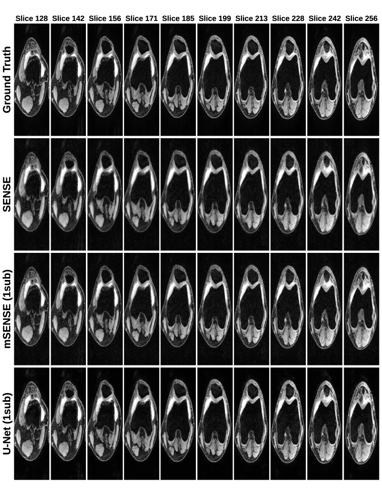
Figure 6: Sample reconstructions at 2x acceleration for the first echo in the SKM-TEA dataset using SENSE, Monarch-SENSE (mSENSE), and U-Net. Both mSENSE and U-Net are trained with 1 training scan. SENSE is an untrained method.

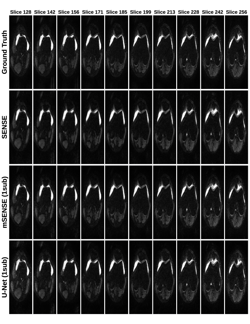
Figure 7: Sample reconstructions at 2x acceleration for the second echo in the SKM-TEA dataset using SENSE, Monarch SENSE (mSENSE), and U-Net. Both mSENSE and U-Net are trained with 1 training scan. SENSE is an untrained method.

References

- Ailon et al. [2021] Ailon, N., Leibovitch, O., and Nair, V. Sparse linear networks with a fixed butterfly structure: theory and practice. In Uncertainty in Artificial Intelligence, pp. 1174–1184. PMLR, 2021.
- Akema et al. [2020] Akema, R., Yamagishi, M., and Yamada, I. Approximate simultaneous diagonalization of matrices via structured low-rank approximation. arXiv preprint arXiv:2010.06305, 2020.
- Bailey [1990] Bailey, D. H. FFTs in external or hierarchical memory. The journal of Supercomputing, 4(1):23–35, 1990.
- Bunse-Gerstner et al. [1993] Bunse-Gerstner, A., Byers, R., and Mehrmann, V. Numerical methods for simultaneous diagonalization. SIAM Journal on Matrix Analysis and Applications, 1993.
- Chaudhari et al. [2020] Chaudhari, A. S., Sandino, C. M., Cole, E. K., Larson, D. B., Gold, G. E., Vasanawala, S. S., Lungren, M. P., Hargreaves, B. A., and Langlotz, C. P. Prospective deployment of deep learning in MRI: A framework for important considerations, challenges, and recommendations for best practices. Journal of Magnetic Resonance Imaging, 2020.
- Chen et al. [2022] Chen, B., Dao, T., Liang, K., Yang, J., Song, Z., Rudra, A., and Ré, C. Pixelated butterfly: Simple and efficient sparse training for neural network models. In International Conference on Learning Representations (ICLR), 2022.
- Child et al. [2019] Child, R., Gray, S., Radford, A., and Sutskever, I. Generating long sequences with sparse transformers. arXiv preprint arXiv:1904.10509, 2019.
- Choromanski et al. [2019] Choromanski, K., Rowland, M., Chen, W., and Weller, A. Unifying orthogonal Monte Carlo methods. In International Conference on Machine Learning, pp. 1203–1212, 2019.
- Cole et al. [2020] Cole, E. K., Pauly, J. M., Vasanawala, S. S., and Ong, F. Unsupervised MRI reconstruction with generative adversarial networks. arXiv preprint arXiv:2008.13065, 2020.
- [10] Conrad, K. The minimal polynomial and some applications.
- Cooley & Tukey [1965] Cooley, J. W. and Tukey, J. W. An algorithm for the machine calculation of complex fourier series. Mathematics of computation, 19(90):297–301, 1965.
- Dao et al. [2019] Dao, T., Gu, A., Eichhorn, M., Rudra, A., and Ré, C. Learning fast algorithms for linear transforms using butterfly factorizations. In International Conference on Machine Learning (ICML), 2019.
- Dao et al. [2020] Dao, T., Sohoni, N., Gu, A., Eichhorn, M., Blonder, A., Leszczynski, M., Rudra, A., and Ré, C. Kaleidoscope: An efficient, learnable representation for all structured linear maps. In International Conference on Learning Representations (ICLR), 2020.
- Darestani & Heckel [2021] Darestani, M. Z. and Heckel, R. Accelerated MRI with un-trained neural networks. IEEE Transactions on Computational Imaging, 7:724–733, 2021.
- Darestani et al. [2021] Darestani, M. Z., Chaudhari, A., and Heckel, R. Measuring robustness in deep learning based compressive sensing. arXiv preprint arXiv:2102.06103, 2021.
- De Sa et al. [2018] De Sa, C., Gu, A., Puttagunta, R., Ré, C., and Rudra, A. A two-pronged progress in structured dense matrix vector multiplication. In Proceedings of the Twenty-Ninth Annual ACM-SIAM Symposium on Discrete Algorithms, pp. 1060–1079. SIAM, 2018.
- Deng et al. [2009] Deng, J., Dong, W., Socher, R., Li, L.-J., Li, K., and Fei-Fei, L. Imagenet: A large-scale hierarchical image database. In 2009 IEEE conference on computer vision and pattern recognition, pp. 248–255. Ieee, 2009.
- Desai et al. [2021a] Desai, A. D., Gunel, B., Ozturkler, B. M., Beg, H., Vasanawala, S., Hargreaves, B. A., Ré, C., Pauly, J. M., and Chaudhari, A. S. Vortex: Physics-driven data augmentations for consistency training for robust accelerated MRI reconstruction. arXiv preprint arXiv:2111.02549, 2021a.
- Desai et al. [2021b] Desai, A. D., Ozturkler, B. M., Sandino, C. M., Vasanawala, S., Hargreaves, B. A., Re, C. M., Pauly, J. M., and Chaudhari, A. S. Noise2recon: A semi-supervised framework for joint MRI reconstruction and denoising. arXiv preprint arXiv:2110.00075, 2021b.
- Desai et al. [2021c] Desai, A. D., Schmidt, A. M., Rubin, E. B., Sandino, C. M., Black, M. S., Mazzoli, V., Stevens, K. J., Boutin, R., Re, C., Gold, G. E., et al. SKM-TEA: A dataset for accelerated MRI reconstruction with dense image labels for quantitative clinical evaluation. In Thirty-fifth Conference on Neural Information Processing Systems Datasets and Benchmarks Track (Round 2), 2021c.
- Dettmers & Zettlemoyer [2019] Dettmers, T. and Zettlemoyer, L. Sparse networks from scratch: Faster training without losing performance. arXiv preprint arXiv:1907.04840, 2019.
- Devlin et al. [2018] Devlin, J., Chang, M.-W., Lee, K., and Toutanova, K. Bert: Pre-training of deep bidirectional transformers for language understanding. arXiv preprint arXiv:1810.04805, 2018.
- Dong et al. [2017] Dong, X., Chen, S., and Pan, S. J. Learning to prune deep neural networks via layer-wise optimal brain surgeon. arXiv preprint arXiv:1705.07565, 2017.
- Dosovitskiy et al. [2020] Dosovitskiy, A., Beyer, L., Kolesnikov, A., Weissenborn, D., Zhai, X., Unterthiner, T., Dehghani, M., Minderer, M., Heigold, G., Gelly, S., et al. An image is worth 16x16 words: Transformers for image recognition at scale. arXiv preprint arXiv:2010.11929, 2020.
- Driscoll et al. [1997] Driscoll, J. R., Healy Jr, D. M., and Rockmore, D. N. Fast discrete polynomial transforms with applications to data analysis for distance transitive graphs. SIAM Journal on Computing, 26(4):1066–1099, 1997.
- Eckart & Young [1936] Eckart, C. and Young, G. The approximation of one matrix by another of lower rank. Psychometrika, 1(3):211–218, 1936.
- Eidelman & Gohberg [1999] Eidelman, Y. and Gohberg, I. On a new class of structured matrices. Integral Equations and Operator Theory, 34(3):293–324, 1999.
- Evci et al. [2019] Evci, U., Pedregosa, F., Gomez, A., and Elsen, E. The difficulty of training sparse neural networks. arXiv preprint arXiv:1906.10732, 2019.
- Fan et al. [2020] Fan, T., Xu, K., Pathak, J., and Darve, E. Solving inverse problems in steady-state navier-stokes equations using deep neural networks. arXiv preprint arXiv:2008.13074, 2020.
- Frankle & Carbin [2018] Frankle, J. and Carbin, M. The lottery ticket hypothesis: Finding sparse, trainable neural networks. arXiv preprint arXiv:1803.03635, 2018.
- Frankle et al. [2019] Frankle, J., Dziugaite, G. K., Roy, D. M., and Carbin, M. Stabilizing the lottery ticket hypothesis. arXiv preprint arXiv:1903.01611, 2019.
- Frankle et al. [2020] Frankle, J., Dziugaite, G. K., Roy, D., and Carbin, M. Linear mode connectivity and the lottery ticket hypothesis. In International Conference on Machine Learning, pp. 3259–3269. PMLR, 2020.
- Gale et al. [2019] Gale, T., Elsen, E., and Hooker, S. The state of sparsity in deep neural networks. arXiv preprint arXiv:1902.09574, 2019.
- Gao et al. [2021] Gao, L., Tow, J., Biderman, S., Black, S., DiPofi, A., Foster, C., Golding, L., Hsu, J., McDonell, K., Muennighoff, N., Phang, J., Reynolds, L., Tang, E., Thite, A., Wang, B., Wang, K., and Zou, A. A framework for few-shot language model evaluation, September 2021. URL https://doi.org/10.5281/zenodo.5371628.
- Geva et al. [2020] Geva, M., Schuster, R., Berant, J., and Levy, O. Transformer feed-forward layers are key-value memories. arXiv preprint arXiv:2012.14913, 2020.
- Gokaslan et al. [2019] Gokaslan, A., Cohen, V., Ellie, P., and Tellex, S. Openwebtext corpus, 2019.
- Gray [2006] Gray, R. M. Toeplitz and circulant matrices: A review. Foundations and Trends® in Communications and Information Theory, 2(3):155–239, 2006.
- Gray et al. [2017] Gray, S., Radford, A., and Kingma, D. P. GPU kernels for block-sparse weights. arXiv preprint arXiv:1711.09224, 3, 2017.
- Griswold et al. [2002] Griswold, M. A., Jakob, P. M., Heidemann, R. M., Nittka, M., Jellus, V., Wang, J., Kiefer, B., and Haase, A. Generalized autocalibrating partially parallel acquisitions (grappa). Magnetic Resonance in Medicine: An Official Journal of the International Society for Magnetic Resonance in Medicine, 47(6):1202–1210, 2002.
- Gu et al. [2020] Gu, A., Dao, T., Ermon, S., Rudra, A., and Ré, C. Hippo: Recurrent memory with optimal polynomial projections. In Advances in neural information processing systems (NeurIPS), 2020.
- Guo et al. [2020] Guo, C., Hsueh, B. Y., Leng, J., Qiu, Y., Guan, Y., Wang, Z., Jia, X., Li, X., Guo, M., and Zhu, Y. Accelerating sparse dnn models without hardware-support via tile-wise sparsity. In SC20: International Conference for High Performance Computing, Networking, Storage and Analysis, pp. 1–15. IEEE, 2020.
- Haldar [2013] Haldar, J. P. Low-rank modeling of local -space neighborhoods (loraks) for constrained MRI. IEEE transactions on medical imaging, 33(3):668–681, 2013.
- Hammernik et al. [2018] Hammernik, K., Klatzer, T., Kobler, E., Recht, M. P., Sodickson, D. K., Pock, T., and Knoll, F. Learning a variational network for reconstruction of accelerated MRI data. Magnetic resonance in medicine, 79(6):3055–3071, 2018.
- Han et al. [2015a] Han, S., Mao, H., and Dally, W. J. Deep compression: Compressing deep neural networks with pruning, trained quantization and huffman coding. arXiv preprint arXiv:1510.00149, 2015a.
- Han et al. [2015b] Han, S., Pool, J., Tran, J., and Dally, W. J. Learning both weights and connections for efficient neural networks. arXiv preprint arXiv:1506.02626, 2015b.
- Han et al. [2016] Han, S., Pool, J., Narang, S., Mao, H., Gong, E., Tang, S., Elsen, E., Vajda, P., Paluri, M., Tran, J., et al. Dsd: Dense-sparse-dense training for deep neural networks. arXiv preprint arXiv:1607.04381, 2016.
- He et al. [2016] He, K., Zhang, X., Ren, S., and Sun, J. Deep residual learning for image recognition. In Proceedings of the IEEE conference on computer vision and pattern recognition, pp. 770–778, 2016.
- Hooker [2020] Hooker, S. The hardware lottery. arXiv preprint arXiv:2009.06489, 2020.
- Hsieh [2003] Hsieh, J. Computed tomography: principles, design, artifacts, and recent advances, volume 114. SPIE press, 2003.
- Jayakumar et al. [2021] Jayakumar, S. M., Pascanu, R., Rae, J. W., Osindero, S., and Elsen, E. Top-KAST: Top-K always sparse training. arXiv preprint arXiv:2106.03517, 2021.
- Jolicoeur-Martineau et al. [2021] Jolicoeur-Martineau, A., Li, K., Piché-Taillefer, R., Kachman, T., and Mitliagkas, I. Gotta go fast when generating data with score-based models. arXiv preprint arXiv:2105.14080, 2021.
- Jurafsky & Martin [2014] Jurafsky, D. and Martin, J. H. Speech and language processing, volume 3. Pearson London, 2014.
- Kailath et al. [1979] Kailath, T., Kung, S.-Y., and Morf, M. Displacement ranks of matrices and linear equations. Journal of Mathematical Analysis and Applications, 68(2):395–407, 1979.
- Kaplan et al. [2020] Kaplan, J., McCandlish, S., Henighan, T., Brown, T. B., Chess, B., Child, R., Gray, S., Radford, A., Wu, J., and Amodei, D. Scaling laws for neural language models. arXiv preprint arXiv:2001.08361, 2020.
- Khalitov et al. [2021] Khalitov, R., Yu, T., Cheng, L., and Yang, Z. Sparse factorization of large square matrices. arXiv preprint arXiv:2109.08184, 2021.
- Kidger et al. [2020] Kidger, P., Morrill, J., Foster, J., and Lyons, T. Neural controlled differential equations for irregular time series. arXiv preprint arXiv:2005.08926, 2020.
- Kingma & Ba [2015] Kingma, D. P. and Ba, J. Adam: A method for stochastic optimization. In International Conference on Learning Representations (ICLR), 2015.
- Knoll et al. [2020] Knoll, F., Hammernik, K., Zhang, C., Moeller, S., Pock, T., Sodickson, D. K., and Akcakaya, M. Deep-learning methods for parallel magnetic resonance imaging reconstruction: A survey of the current approaches, trends, and issues. IEEE signal processing magazine, 37(1):128–140, 2020.
- Kochkov et al. [2021] Kochkov, D., Smith, J. A., Alieva, A., Wang, Q., Brenner, M. P., and Hoyer, S. Machine learning–accelerated computational fluid dynamics. Proceedings of the National Academy of Sciences, 118(21), 2021.
- Lagunas et al. [2021] Lagunas, F., Charlaix, E., Sanh, V., and Rush, A. M. Block pruning for faster transformers. arXiv preprint arXiv:2109.04838, 2021.
- Lahiri et al. [2021] Lahiri, A., Wang, G., Ravishankar, S., and Fessler, J. A. Blind primed supervised (blips) learning for mr image reconstruction. arXiv preprint arXiv:2104.05028, 2021.
- Le et al. [2013] Le, Q., Sarlós, T., and Smola, A. Fastfood-computing hilbert space expansions in loglinear time. In International Conference on Machine Learning, pp. 244–252, 2013.
- Le Magoarou & Gribonval [2016] Le Magoarou, L. and Gribonval, R. Flexible multilayer sparse approximations of matrices and applications. IEEE Journal of Selected Topics in Signal Processing, 10(4):688–700, 2016.
- Li et al. [2016] Li, H., Kadav, A., Durdanovic, I., Samet, H., and Graf, H. P. Pruning filters for efficient convnets. arXiv preprint arXiv:1608.08710, 2016.
- Li et al. [2020] Li, Z., Kovachki, N. B., Azizzadenesheli, K., Bhattacharya, K., Stuart, A., Anandkumar, A., et al. Fourier neural operator for parametric partial differential equations. In International Conference on Learning Representations, 2020.
- Lin et al. [2017] Lin, J., Rao, Y., Lu, J., and Zhou, J. Runtime neural pruning. In Guyon, I., Luxburg, U. V., Bengio, S., Wallach, H., Fergus, R., Vishwanathan, S., and Garnett, R. (eds.), Advances in Neural Information Processing Systems, volume 30. Curran Associates, Inc., 2017.
- Lin et al. [2021] Lin, R., Ran, J., Chiu, K. H., Chesi, G., and Wong, N. Deformable butterfly: A highly structured and sparse linear transform. Advances in Neural Information Processing Systems, 34, 2021.
- Liu & Zenke [2020] Liu, T. and Zenke, F. Finding trainable sparse networks through neural tangent transfer. In International Conference on Machine Learning, pp. 6336–6347. PMLR, 2020.
- Lustig et al. [2007] Lustig, M., Donoho, D., and Pauly, J. M. Sparse MRI: The application of compressed sensing for rapid mr imaging. Magnetic Resonance in Medicine: An Official Journal of the International Society for Magnetic Resonance in Medicine, 58(6):1182–1195, 2007.
- Mardani et al. [2018] Mardani, M., Gong, E., Cheng, J. Y., Vasanawala, S. S., Zaharchuk, G., Xing, L., and Pauly, J. M. Deep generative adversarial neural networks for compressive sensing MRI. IEEE transactions on medical imaging, 38(1):167–179, 2018.
- Massaroli et al. [2021] Massaroli, S., Poli, M., Sonoda, S., Suzuki, T., Park, J., Yamashita, A., and Asama, H. Differentiable multiple shooting layers. arXiv preprint arXiv:2106.03885, 2021.
- Mattson et al. [2020] Mattson, P., Cheng, C., Diamos, G., Coleman, C., Micikevicius, P., Patterson, D., Tang, H., Wei, G.-Y., Bailis, P., Bittorf, V., et al. Mlperf training benchmark. Proceedings of Machine Learning and Systems, 2:336–349, 2020.
- Merity et al. [2016] Merity, S., Xiong, C., Bradbury, J., and Socher, R. Pointer sentinel mixture models. arXiv preprint arXiv:1609.07843, 2016.
- Moczulski et al. [2016] Moczulski, M., Denil, M., Appleyard, J., and de Freitas, N. ACDC: a structured efficient linear layer. In International Conference on Learning Representations, 2016.
- Morcos et al. [2019] Morcos, A. S., Yu, H., Paganini, M., and Tian, Y. One ticket to win them all: generalizing lottery ticket initializations across datasets and optimizers. arXiv preprint arXiv:1906.02773, 2019.
- Munkhoeva et al. [2018] Munkhoeva, M., Kapushev, Y., Burnaev, E., and Oseledets, I. Quadrature-based features for kernel approximation. In Bengio, S., Wallach, H., Larochelle, H., Grauman, K., Cesa-Bianchi, N., and Garnett, R. (eds.), Advances in Neural Information Processing Systems 31, pp. 9165–9174. Curran Associates, Inc., 2018.
- Ong & Lustig [2016] Ong, F. and Lustig, M. Beyond low rank+ sparse: Multiscale low rank matrix decomposition. IEEE journal of selected topics in signal processing, 10(4):672–687, 2016.
- Orseau et al. [2020] Orseau, L., Hutter, M., and Rivasplata, O. Logarithmic pruning is all you need. Advances in Neural Information Processing Systems, 33, 2020.
- Pan [2012] Pan, V. Y. Structured matrices and polynomials: unified superfast algorithms. Springer Science & Business Media, 2012.
- Parker [1995] Parker, D. S. Random butterfly transformations with applications in computational linear algebra. 1995.
- Pensia et al. [2020] Pensia, A., Rajput, S., Nagle, A., Vishwakarma, H., and Papailiopoulos, D. Optimal lottery tickets via subsetsum: Logarithmic over-parameterization is sufficient. arXiv preprint arXiv:2006.07990, 2020.
- Peste et al. [2021] Peste, A., Iofinova, E., Vladu, A., and Alistarh, D. Ac/dc: Alternating compressed/decompressed training of deep neural networks. Advances in Neural Information Processing Systems, 34, 2021.
- Poli et al. [2020] Poli, M., Massaroli, S., Yamashita, A., Asama, H., Park, J., et al. Hypersolvers: Toward fast continuous-depth models. Advances in Neural Information Processing Systems, 33, 2020.
- Pruessmann et al. [1999] Pruessmann, K. P., Weiger, M., Scheidegger, M. B., and Boesiger, P. Sense: sensitivity encoding for fast MRI. Magnetic Resonance in Medicine: An Official Journal of the International Society for Magnetic Resonance in Medicine, 42(5):952–962, 1999.
- Rackauckas et al. [2020] Rackauckas, C., Ma, Y., Martensen, J., Warner, C., Zubov, K., Supekar, R., Skinner, D., Ramadhan, A., and Edelman, A. Universal differential equations for scientific machine learning. arXiv preprint arXiv:2001.04385, 2020.
- Radford et al. [2019] Radford, A., Wu, J., Child, R., Luan, D., Amodei, D., Sutskever, I., et al. Language models are unsupervised multitask learners. OpenAI blog, 1(8):9, 2019.
- Raissi et al. [2019] Raissi, M., Perdikaris, P., and Karniadakis, G. E. Physics-informed neural networks: A deep learning framework for solving forward and inverse problems involving nonlinear partial differential equations. Journal of Computational Physics, 378:686–707, 2019.
- Rasley et al. [2020] Rasley, J., Rajbhandari, S., Ruwase, O., and He, Y. Deepspeed: System optimizations enable training deep learning models with over 100 billion parameters. In Proceedings of the 26th ACM SIGKDD International Conference on Knowledge Discovery & Data Mining, pp. 3505–3506, 2020.
- Ravishankar et al. [2017] Ravishankar, S., Moore, B. E., Nadakuditi, R. R., and Fessler, J. A. Low-rank and adaptive sparse signal (lassi) models for highly accelerated dynamic imaging. IEEE transactions on medical imaging, 36(5):1116–1128, 2017.
- Ronneberger et al. [2015] Ronneberger, O., Fischer, P., and Brox, T. U-net: Convolutional networks for biomedical image segmentation. In International Conference on Medical image computing and computer-assisted intervention, pp. 234–241. Springer, 2015.
- Sandino et al. [2020] Sandino, C. M., Cheng, J. Y., Chen, F., Mardani, M., Pauly, J. M., and Vasanawala, S. S. Compressed sensing: From research to clinical practice with deep neural networks: Shortening scan times for magnetic resonance imaging. IEEE signal processing magazine, 37(1):117–127, 2020.
- Sanh et al. [2020] Sanh, V., Wolf, T., and Rush, A. M. Movement pruning: Adaptive sparsity by fine-tuning. arXiv preprint arXiv:2005.07683, 2020.
- Schönemann [1966] Schönemann, P. H. A generalized solution of the orthogonal procrustes problem. Psychometrika, 31(1):1–10, 1966.
- Shoeybi et al. [2019] Shoeybi, M., Patwary, M., Puri, R., LeGresley, P., Casper, J., and Catanzaro, B. Megatron-LM: Training multi-billion parameter language models using model parallelism. arXiv preprint arXiv:1909.08053, 2019.
- Sindhwani et al. [2015] Sindhwani, V., Sainath, T., and Kumar, S. Structured transforms for small-footprint deep learning. In Advances in Neural Information Processing Systems, pp. 3088–3096, 2015.
- Tanaka et al. [2020] Tanaka, H., Kunin, D., Yamins, D. L., and Ganguli, S. Pruning neural networks without any data by iteratively conserving synaptic flow. arXiv preprint arXiv:2006.05467, 2020.
- Tewarson [1973] Tewarson, R. P. Sparse matrices, volume 69. Academic Press New York, 1973.
- Thomas et al. [2018] Thomas, A., Gu, A., Dao, T., Rudra, A., and Ré, C. Learning compressed transforms with low displacement rank. In Advances in neural information processing systems, pp. 9052–9060, 2018.
- Tolstikhin et al. [2021] Tolstikhin, I., Houlsby, N., Kolesnikov, A., Beyer, L., Zhai, X., Unterthiner, T., Yung, J., Keysers, D., Uszkoreit, J., Lucic, M., et al. Mlp-Mixer: An all-mlp architecture for vision. arXiv preprint arXiv:2105.01601, 2021.
- Trefethen [2000] Trefethen, L. N. Spectral methods in MATLAB. SIAM, 2000.
- Vahid et al. [2020] Vahid, K. A., Prabhu, A., Farhadi, A., and Rastegari, M. Butterfly transform: An efficient fft based neural architecture design. In 2020 IEEE/CVF Conference on Computer Vision and Pattern Recognition (CVPR), pp. 12021–12030. IEEE, 2020.
- Wang et al. [2020a] Wang, C., Zhang, G., and Grosse, R. Picking winning tickets before training by preserving gradient flow. arXiv preprint arXiv:2002.07376, 2020a.
- Wang et al. [2020b] Wang, R., Kashinath, K., Mustafa, M., Albert, A., and Yu, R. Towards physics-informed deep learning for turbulent flow prediction. In Proceedings of the 26th ACM SIGKDD International Conference on Knowledge Discovery & Data Mining, pp. 1457–1466, 2020b.
- Wolf et al. [2020] Wolf, T., Debut, L., Sanh, V., Chaumond, J., Delangue, C., Moi, A., Cistac, P., Rault, T., Louf, R., Funtowicz, M., Davison, J., Shleifer, S., von Platen, P., Ma, C., Jernite, Y., Plu, J., Xu, C., Scao, T. L., Gugger, S., Drame, M., Lhoest, Q., and Rush, A. M. Transformers: State-of-the-art natural language processing. In Proceedings of the 2020 Conference on Empirical Methods in Natural Language Processing: System Demonstrations, pp. 38–45, Online, October 2020. Association for Computational Linguistics. URL https://www.aclweb.org/anthology/2020.emnlp-demos.6.
- Yaman et al. [2020] Yaman, B., Hosseini, S. A. H., Moeller, S., Ellermann, J., Uğurbil, K., and Akçakaya, M. Self-supervised physics-based deep learning MRI reconstruction without fully-sampled data. In 2020 IEEE 17th International Symposium on Biomedical Imaging (ISBI), pp. 921–925. IEEE, 2020.
- Yu et al. [2016] Yu, F. X., Suresh, A. T., Choromanski, K. M., Holtmann-Rice, D. N., and Kumar, S. Orthogonal random features. In Lee, D. D., Sugiyama, M., Luxburg, U. V., Guyon, I., and Garnett, R. (eds.), Advances in Neural Information Processing Systems 29, pp. 1975–1983. Curran Associates, Inc., 2016.
- Yuan et al. [2021] Yuan, L., Chen, Y., Wang, T., Yu, W., Shi, Y., Tay, F. E., Feng, J., and Yan, S. Tokens-to-token ViT: Training vision transformers from scratch on imagenet. arXiv preprint arXiv:2101.11986, 2021.
- Zhao et al. [2021] Zhao, T. Z., Wallace, E., Feng, S., Klein, D., and Singh, S. Calibrate before use: Improving few-shot performance of language models. arXiv preprint arXiv:2102.09690, 2021.
- Zhu & Gupta [2017] Zhu, M. and Gupta, S. To prune, or not to prune: exploring the efficacy of pruning for model compression. arXiv preprint arXiv:1710.01878, 2017.
- Zhu et al. [2015] Zhu, Y., Kiros, R., Zemel, R., Salakhutdinov, R., Urtasun, R., Torralba, A., and Fidler, S. Aligning books and movies: Towards story-like visual explanations by watching movies and reading books. In Proceedings of the IEEE international conference on computer vision, pp. 19–27, 2015.