Reach and complementarity of $\mu\to e$ searches

Abstract

In Effective Field Theory, we describe $\mu\leftrightarrow e$ flavour changing transitions using an operator basis motivated by experimental observables. In a six-dimensional subspace probed by $\mu\to e\gamma$, $\mu\to e\bar{e}e$ and $\mu\to e$ conversion on nuclei, we derive constraints on the New Physics scale from past and future experiments, illustrating the complementarity of the processes in an intuitive way. We also recall that a precise determination of the scalar quark currents in the nucleon will be required to distinguish scalar $\mu\to e$ interactions on $u$-quarks from those on $d$-quarks.

I Introduction

Lepton flavor-violating contact interactions — referred to as LFV or CLFV — are excellent probes of physics beyond the standard model (see e.g. KO ; Calibbi for reviews). The non-zero neutrino masses and mixing angles imply their existence, and an observation could shed light on the neutrino mass mechanism mnu , and even on the matter excess of our universe if generated via leptogenesis Y+ ; PRep . The rates could be just below the current experimental bounds, in many extensions of the Standard Model that introduce additional CLFV sources Calibbi .

CLFV searches have been conducted in a wide range of reactions, and a subset of current and anticipated experimental constraints are given in Table 1. While the multitude of $\tau$ channels could contribute to identifying the nature of New Physics (NP), the greater sensitivity in muon sector seems more promising for discovering it. Although the number of muon processes is limited, the corresponding bounds are already quite restrictive, and exceptional improvements are expected in the coming years.

process	current sensitivity	future
$\mu\to e\gamma$	$<4.2\times 10^{-13}$(MEG TheMEG:2016wtm )	$\sim 10^{-14}$ (MEG II MEGII )
$\mu\to e\bar{e}e$	$<1.0\times 10^{-12}$(SINDRUM Bellgardt:1987du )	$\sim 10^{-16}$ (Mu3e Mu3e )
$\mu$A$\to e$A	$<7\times 10^{-13}$(SINDRUM II Bertl:2006up )	$\sim 10^{-16}$ (COMET COMET , Mu2e mu2e )
		$\sim 10^{-(18\to 20)}$ (PRISM/PRIME PP )
$\tau\to l\gamma$	$<3.3\times 10^{-8}$(Babar) tau1	$\sim 10^{-9}$(BelleII) belle2t3l
$\tau\to 3l$	$<$ few$\times 10^{-8}$ (Belle) tau2	$\sim 10^{-9}$(BelleII) belle2t3l
$\tau\to l\pi^{0}$	$<8.0\times 10^{-8}$ (Belle) Belle:2007cio	$\sim 10^{-9}$ (BelleII) belle2t3l
$\tau\to l\rho$	$<1.2\times 10^{-8}$ (Belle) Belle:2007cio	$\sim 10^{-9}$ (BelleII) belle2t3l

Table 1: Current bounds on the branching ratios for various lepton flavour changing processes, and the expected reach of upcoming experiments.

The reach and complementarity of $\mu\to e\gamma$, $\mu\to e\bar{e}e$ and $\mu A\!\to\!eA$ transitions have been explored from various perspectives. Numerous authors have investigated model preferences and predictions for correlations among CLFV observables everyone . An early model-independent analysis was performed by de Gouvea and Vogel deGouvea , using a simple effective Lagrangian to describe NP effects. The presentation of our results follows their intuitive plots. However, their approach was limited to comparing the reach of pairs of processes (e.g. $\mu\to e\gamma$ vs. $\mu A\!\to\!eA$) at tree level. More systematic Effective Field Theory (EFT) studies, including more operators and some loop effects, were performed in PSI ; C+C ; PSI focused on the sensitivity of the processes to a more complete operator basis, and C+C explored whether the proposed experimental muon program is necessary and sufficient to find $\mu\to e$ flavour change.

The aim of this work is to graphically illustrate the complementarity and reach of the $\mu\to e\gamma$, $\mu\to e\bar{e}e$ and $\mu A\!\to\!eA$ processes. We describe the physics of CLFV in an EFT perspective Georgi ; burashouches ; LesHouches , where the number of operator coefficients is reduced by choosing an operator basis motivated by our observables C+C . We quantify complementarity as the degree to which observables probe different operator coefficients, and study the complementarity of observables at the New Physics scale because the aim is to make observations that give distinct information at $\Lambda_{LFV}$. The coefficients are translated to $\Lambda_{LFV}$ using Renormalisation Group Equations. This study extends the analysis described in C+C in several ways: we provide more informative plots of the current and projected experimental reaches, and a more rigorous construction of the basis for the subspace of experimentally accessible operator coefficients. In addition we draw attention to the information loss in matching nucleons to quarks using current theoretical results. Using this formalism to study whether $\mu\to e$ processes can distinguish among models is an interesting question that we leave for a subsequent publication.

This paper is organized as follows: section II outlines the procedure to take the data parametrized in EFT from the experimental scale to beyond the weak scale. Section III presents constraints from various experimental measurements and projections for future initiatives. The construction of the basis used in this work is discussed in Appendices A and B. An independent issue regarding information loss in relating $\mu A\!\to\!eA$ rates to models is finally discussed in section IV.

II Theory overview

This section gives the Lagrangian and Branching Ratios at the experimental scale, and sketches the transformation of operator coefficients from the experimental scale to $\Lambda_{LFV}$ (which is described in more detail in  C+C ).

A challenge of the EFT approach lies in the large number of operators. In the case of $\mu\to e$ flavour changing processes, about 90 operators C+C are required to parametrize interactions that have $\leq 4$ Standard Model legs at low energy and are otherwise flavour-diagonal. The difficulty to constrain and visualize this high-dimensional space is compounded by the fact that there are (only) three processes with excellent sensitivity in the $\mu\to e$ sector (see Table 1), imposing only about a dozen constraints on operator coefficients DKY . Improved theoretical calculations and additional $\mu A\!\to\!eA$ measurements with different nuclear targets could increase this number to $\sim 20$ independent constraints DKY . Determining all EFT coefficients appears therefore a daunting task.

This manuscript takes a different perspective, following C+C . Since there are three processes with excellent experimental sensitivity, we restrict to the (12-dimensional) subspace of operator coefficients probed by $\mu\to e\gamma,\mu\to e\bar{e}e$, and Spin Independent $\mu Al\to eAl$ and $\mu Au\to eAu$. The dimension of the subspace can be further reduced by half since the operator coefficients can be labelled by the helicity (or chirality) of the outgoing relativistic electron, and the results are very similar for either $e_{L}$ or $e_{R}$, which do not interfere. Restricting the analysis to the subspace corresponding to an outgoing $e_{L}$, the three muon processes can be described at the experimental scale ($\sim m_{\mu}$) by the following effective Lagrangian KO :

$$\delta{\cal L} = \frac{1}{\Lambda_{LFV}^{2}}{\Big{[}}C_{D}(\overline{e}\sigma^{\alpha\beta}P_{R}\mu)F_{\alpha\beta}+C_{S}(\overline{e}P_{R}\mu)(\overline{e}P_{R}e)+C_{VR}(\overline{e}\gamma^{\alpha}P_{L}\mu)(\overline{e}\gamma_{\alpha}P_{R}e)$$ (II.1)

$$\phantom{\frac{1}{\Lambda_{LFV}^{2}}{\Big{[}}}+C_{VL}(\overline{e}\gamma^{\alpha}P_{L}\mu)(\overline{e}\gamma_{\alpha}P_{L}e)+C_{Alight}{\cal O}_{Alight}+C_{Aheavy\perp}{\cal O}_{Aheavy\perp}{\Big{]}}$$

where $\Lambda_{LFV}$ is a heavy mass scale, and the dimensionless coefficients $\{C_{Z}\}$ are lined up in a vector $\vec{C}$. The first term of this Lagrangian is a dipole operator mediating $\mu\to e\gamma$ and contributing to both $\mu\to e\bar{e}e$ and $\mu A\!\to\!eA$. The next three contact operators contribute to $\mu\to e\bar{e}e$, while ${\cal O}_{Alight}$ is a combination of operators probed by light muon conversion targets such as Ti or Al, and ${\cal O}_{Aheavy\perp}$ is an orthogonal combination probed by heavy targets such as Au. We take Au and Al as prototypical “heavy” and “light” targets since Au was used by the SINDRUM experiment Bertl:2006up , and Al will be used by the upcoming COMET COMET and Mu2e mu2e experiments, in addition to resembling Ti used in the past Bertl:2006up .

The constraint on the dipole operator from $\mu\to e\gamma$ is given by:

$$BR(\mu\to e_{L}\gamma) = 384\pi^{2}\frac{v^{4}}{\Lambda_{LFV}^{4}}|\vec{C}\cdot\hat{e}_{DR}|^{2}<B_{\mu\to e\gamma}^{expt}=4.2\times 10^{-13}$$ (II.2)

where we introduced unit vectors $\hat{e}_{A}$ which select coefficients $C_{A}$ in the six-dimensional subspace. The four-lepton operators do not interfere with each other in $\mu\to e\bar{e}e$ since the electrons are relativistic ($\approx$ chiral), setting the three following constraints:

$$BR(\mu\to e_{L}\overline{e_{R}}e_{L}) = \frac{v^{4}}{\Lambda_{LFV}^{4}}\frac{|\vec{C}\cdot\hat{e}_{S}|^{2}}{8}\leq B^{expt}_{\mu\to e\bar{e}e}=10^{-12}$$ (II.3)

$$BR(\mu\to e_{L}\overline{e_{L}}e_{L}) = \frac{v^{4}}{\Lambda_{LFV}^{4}}\left[2|\vec{C}\cdot\hat{e}_{VL}+4e\vec{C}\cdot\hat{e}_{D}|^{2}+e^{2}(32\ln\frac{m_{\mu}}{m_{e}}-68)|\vec{C}\cdot\vec{e}_{D}|^{2}\right]\leq B_{\mu\to e\bar{e}e}^{expt}$$

$$BR(\mu\to e_{L}\overline{e_{R}}e_{R}) = \frac{v^{4}}{\Lambda_{LFV}^{4}}\left[|\vec{C}\cdot\hat{e}_{VR}+4e\vec{C}\cdot\hat{e}_{D}|^{2}+e^{2}(32\ln\frac{m_{\mu}}{m_{e}}-68)|\vec{C}\cdot\hat{e}_{D}|^{2}\right]\leq B_{\mu\to e\bar{e}e}^{expt}~{}~{}~{}.$$

These can conveniently be summarised as

$$BR(\mu\to e_{L}\bar{e}e)=\frac{v^{4}}{\Lambda_{LFV}^{4}}\vec{C}^{\dagger}\bm{R}_{\mu\to e_{L}\bar{e}e}\vec{C}\leq B_{\mu\to e\bar{e}e}^{expt}$$ (II.4)

where the matrix R${}_{\mu\to e_{L}\bar{e}e}$ is proportional to the inverse covariance matrix for $\mu\to e\bar{e}e$, given in eqn (A.7). Similarly, the Conversion Ratios for $\mu A\!\to\!eA$ can be written

$$CR(\mu Al\to e_{L}Al) = \frac{v^{4}}{\Lambda_{LFV}^{4}}\vec{C}^{\dagger}\bm{R}_{\mu{\rm Al}\to e_{L}{\rm Al}}\vec{C}\leq B_{\mu Al\to eAl}^{expt}$$

$$CR(\mu Au\to e_{L}Au) = \frac{v^{4}}{\Lambda_{LFV}^{4}}\vec{C}^{\dagger}\bm{R}_{\mu{\rm Au}\to e_{L}{\rm Au}}\vec{C}\leq B_{\mu Au\to eAu}^{expt}$$ (II.5)

where the R matrices are given in eqn (A.13). These expressions justify a posteriori the basis in eqn (II.1), chosen to be orthogonal, intuitive, and correspond closely to the coefficient combinations probed by observables. The eigenvectors of the covariance matrix could be another basis choice, discussed briefly in Appendix B.3.

From the Lagrangian (II.1), one can easily deduce that the three processes are complementary at the experimental scale: four-fermion interactions with leptons only contribute to $\mu\to e\bar{e}e$, interactions with strongly-interacting particles only contribute to $\mu A\!\to\!eA$ (the complementarity between heavy or light targets is discussed at the end of Appendix A), while the dipole contributes to all processes. The complementarity of two processes can be interpreted geometrically as the misalignment between the corresponding vectors in coefficient space, defined as the angle $\eta$ between the two vectors. In terms of R matrices, the complementarity between processes $A$ and $B$ can be expressed as:

$$\cos\eta\sim\frac{{\rm Tr}{\Big{[}}\bm{R}_{A}\bm{R}_{B}{\Big{]}}}{{\rm Tr}{\Big{[}}\bm{R}_{A}{\Big{]}}{\rm Tr}{\Big{[}}\bm{R}_{B}{\Big{]}}}~{}~{}~{},$$ (II.6)

which vanishes for perfectly complementary observables, and is equal to one when they contain the same information. The basis in eqn (II.1) was chosen to be perfectly complementary, i.e. orthogonal, at the experimental scale.

In the following, we adopt a different approach to illustrate the complementarity between processes. Instead of using the geometric measure defined above, we show that each process gives independent information about the operator coefficients by plotting the corresponding reach separately. The measured rates can then be combined to identify a point in parameter space.

The degree of complementarity can be evaluated at $\Lambda_{LFV}$ by translating the coefficients in eqn (II.1) from the experimental scale to $\Lambda_{LFV}$. Modifying the scale amounts to changing the separation between lower energy loop effects that are explicitly calculated, and higher energy loops that are implicitly resummed into the coupling constants. At the experimental scale, all the loops via which a New Physics model contributes to an observable are in the operator coefficients, and the rate is straightforward to calculate. On the other hand, the operator coefficients at the heavy LFV scale are easily derived from a New Physics model, but loops must be calculated to evaluate experimental quantities. So the low-energy operator coefficients of eqn ( II.1) can be transformed to the LFV scale $\Lambda_{LFV}$ via the Renormalisation Group Equations (RGEs) PSI ; JMT , which peel off the SM loops in a leading log expansion. Solving the RGEs perturbatively, and modifying the EFT with scale to account for the changing particle content, allows us to write

$$\vec{C}(m_{\mu})=\bm{G}^{T}(\Lambda_{LFV},m_{\mu})\vec{C}(\Lambda_{LFV})~{}~{}~{}.$$ (II.7)

The matrix G is similar to that given in C+C . We neglect loop effects in the EFT of nucleons and pions and match at 2 GeV onto a QCD-invariant EFT with gluons and five flavours of quarks (see Appendix A and Table 3). The leading log QED and QCD effects are included up to $m_{W}$ PSI ; Roma , where the coefficients are matched (at tree level in the lower-energy EFT) onto dimension six SMEFT operators, augmented by the dimension eight scalar operator Murphy ; autredim8 corresponding to $\hat{e}_{S}$, which could be relevant powercount . We neglected CKM angles in matching and some other relevant SMEFT operators of dimension eight, and stress that the running from $m_{W}\to\Lambda_{LFV}$ is not included.

The Branching Ratios in terms of coefficients at $\Lambda_{LFV}$ can be expressed as:

$$BR(\mu\to e_{L}X) = \vec{C}^{\dagger}(m_{W})\bm{G}^{*}(m_{W},m_{\mu})\bm{R}_{\mu\to e_{L}X}(m_{\mu})\bm{G}^{T}(m_{W},m_{\mu})\vec{C}(m_{W})$$ (II.8)

where the matrix G is not unitary, and does not preserve the orthonormality of the basis since SM loops and matching can change the normalisation and direction of the vectors $\{\hat{e}_{A}\}$. This is expected since distinct observations at low energy can measure the same high-scale NP coefficients. The changing modulus of the basis vectors is simple to calculate and include, and affects the reach. The changes in direction can affect the complementarity of processes if the vectors become more or less aligned (see Appendix  B).

III Illustrating experimental constraints

In this section, we illustrate the constraints on New Physics from current and future $\mu\to e$ searches, and show how these results can be combined to identify the allowed region of coefficient space. We parametrize the coefficient space with spherical coordinates sphcoord (Table 2) assuming that the vector of coefficients $\vec{C}$ is normalised to unity at the experimental scale. The reach of the various experiments in $\Lambda_{LFV}$ can be calculated as a function of these angles and the branching ratios given in eqn B.3. We stress that we are showing (projected) exclusion curves, as opposed to “one-at-a-time” bounds, since our EFT formulation should account for potential cancellations in the theoretical rate.

In deriving this parametrization, we approximating the operator coefficients as real numbers. This familiar simplification reduces our coefficient space from six complex to six real dimensions, replacing relative phases between interfering coefficients with a relative sign. Furthermore, we focus on a four-dimensional subspace, corresponding approximately to the four processes we examine, by suppressing two of the three four-lepton directions (the four-lepton operators can be distinguished by measuring the angular distribution in $\mu\to e\bar{e}e$ Okadameee ). The direction $\vec{e}_{S}$ associated to the scalar four lepton operator interferes with none of the other operators and receives negligible loop corrections, so it is complementary by inspection. We also neglect a linear combination of the vector four-lepton directions $\vec{e}_{VR}$ and $\vec{e}_{VL}$, since their contributions to $\mu\to e\bar{e}e$ have similar form. A judicious choice ensures the approximate orthogonality of the remaining four basis vectors. The full details are given in Appendix B.

$\vec{C}\cdot\vec{e}_{D}$	$|\vec{e}_{D}|\cos\theta_{D}$
$\vec{C}\cdot\vec{e}_{S}$	$|\vec{e}_{S}|\sin\theta_{D}\cos\theta_{S}$
$\vec{C}\cdot\vec{e}_{VL}$	$|\vec{e}^{{}^{\prime}}_{VL}|\sin\theta_{D}\sin\theta_{S}\cos\theta_{V}$
$\vec{C}\cdot\vec{e}_{VR}$	$|\vec{e}^{{}^{\prime}}_{VR}|\sin\theta_{D}\sin\theta_{S}\cos\theta_{V}$
$\vec{C}\cdot\vec{e}_{Alight}$	$|\vec{e}_{Alight}|\sin\theta_{D}\sin\theta_{S}\sin\theta_{V}\sin\phi$
$\vec{C}\cdot\vec{e}_{Aheavy\perp}$	$|\vec{e}_{Aheavy\perp}|\sin\theta_{D}\sin\theta_{S}\sin\theta_{V}\cos\phi$

Table 2: Dimensionless operator coefficients expressed in the angular coordinates. The radial coordinate is $1/\Lambda_{LFV}^{2}$, $\theta_{I}:0..\pi$ and $\phi:0..2\pi$. As discussed in Appendix B.1, the $\vec{e}_{VL}\times\vec{e}_{VR}$ plane was projected to a line, deviations from which are measured by $\theta_{V}$. In general, the basis vectors $\{e_{A}\}$ are not unit vectors, and their normalisation is given in Table 5 and after eqn (B.3) for the primed vectors.

We plot in Figure 1 the reach of $\mu\to e_{L}\gamma$, $\mu\to e_{L}\bar{e}e$ and $\mu{\rm Al}\to e_{L}{\rm Al}$ as a function of $\theta_{D}$ for $\theta_{S}=\pi/2$, $\theta_{V}=\pi/4$, and $\phi=\pi/4$. This corresponds to $\vec{C}\cdot\vec{e}_{S}=0$, so $\mu\to e\bar{e}e$ induced by the $\vec{C}\cdot\vec{e}_{D}$, $\vec{C}\cdot\vec{e}_{VR}$ and $\vec{C}\cdot\vec{e}_{VL}$, and $\mu A\!\to\!eA$ probed by Al and Au. At $\theta_{D}=0,$ the dipole coefficient is only contribution to the rates. At $\theta_{D}=\pi/2$, $\vec{C}\cdot\vec{e}_{D}$ vanishes (so does $\mu\to e\gamma$) and $\mu\to e\bar{e}e$ and $\mu A\!\to\!eA$ are purely mediated by four-fermion operators. For $\theta_{D}>\pi/2$, $\vec{C}\cdot\vec{e}_{D}$ is negative and $\mu A\!\to\!eA$ vanishes when the dipole contribution cancels the remaining contributions. The rate drops abruptly, indicating that the dipole contribution is relatively small and the cancellation only occurs in a narrow region. The valley is broader for $\mu\to e\bar{e}e$, since the contribution of $\vec{C}\cdot\vec{e}_{D}$ is more important, and the rate never vanishes because $\mu\to e\bar{e}e$ independently constrains each coefficient contributing to this process, so the rate only vanishes when all the coefficients do (see eqn  II.3).

Our angular coordinate parametrisation defined a measure on the parameter space that assumes all the coefficients in our subspace are ${\cal O}(1)$ once the scale $\Lambda_{LFV}$ is fixed. This might not be the case in some classes of models; for instance $\vec{C}\cdot\vec{e}_{D}\gg$ four-fermion coefficients can occur (in SUSY Hisano:1996qq ), or the dipole could be suppressed, when the four-fermion operators are generated at tree level. To illustrate complementarity when the “natural” size of $\vec{C}\cdot\vec{e}_{D}$ is orders of magnitude different from the other coefficients, we also plot the reach in a parametrization similar to that introduced in deGouvea by defining a variable

$$\kappa_{D}={\rm cotan}(\theta_{D}-\pi/2)~{}~{}~{}.$$ (III.1)

This non-linear transformation magnifies the regions where the dipole contribution either dominates the four-fermion interactions ($\theta=0,\pi$) or is suppressed ($\theta=\pi/2$). We also define a similar variable $\kappa_{V}$, that magnifies the regions where leptonic four-fermion coefficients are much larger or smaller than those with quarks. We subtract $\pi/2$ in order to have $\mu\to e\gamma$ larger at the centre of the plot, following deGouvea . However, this choice means that $\kappa$=0 corresponds to both to $\theta$ = 0 and $\theta=\pi$, and the rates can be discontinuous at 0 while they are continuous at $\pm\infty$. This can be observed in figure 3.

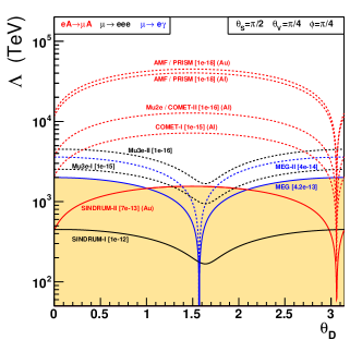
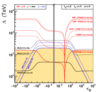
Figure 1: Reach as a function of (left) the angle $\theta_{D}$, which parametrizes the relative magnitude of dipole and four-fermion coefficients, and (right) the variable $\kappa_{D}={\rm cotan}(\theta_{D}-\pi/2)$. The scale $\Lambda$ is defined in eqn (II.1) with the coefficients normalised according to Table 2. The solid region is currently excluded.

Figure 2 displays the reach as a function of $\theta_{V}$, which is effectively the angle between the $\mu\to e\bar{e}e$ and $\mu A\!\to\!eA$ four-fermion operators. Results for a vanishing dipole contribution ($\theta_{D}=\pi/2$) shows that $\mu\to e\bar{e}e$ vanishes at $\theta_{V}=\pi/2$ and $\mu A\!\to\!eA$ at $\theta_{V}=0,\pi$. Adding a small negative dipole coefficient, $\mu\to e\bar{e}e$ doesn’t vanish anymore since the dipole contributes independently as well as in interference with the four-fermion contributions, and the rate is reduced when this interference is destructive. The magnitude of the negative dipole coefficient is larger for $\theta_{D}=3\pi/4$, exhibiting that $\mu A\!\to\!eA$ vanishes when the dipole cancels the four-fermion contributions. Similar plots for $\kappa_{V}={\rm cotan}(\theta_{V}-\pi/2)$ are shown in Figure 3.

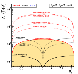
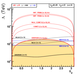
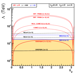
Figure 2: Reach as a function of the angle $\theta_{V}$, which is effectively the angle between the $\mu\to e\bar{e}e$ and $\mu A\!\to\!eA$ four-fermion operators, for different contributions of the dipole operator: (left) $\theta_{D}=\pi/2$, (middle) $\theta_{D}=5\pi/9$, and (right) $\theta_{D}=3\pi/4$. The solid region is currently excluded.

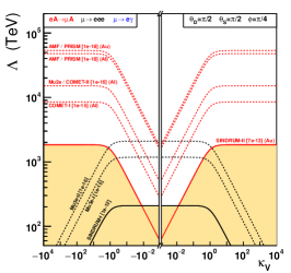
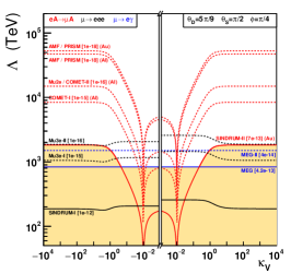
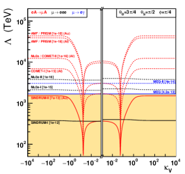
Figure 3: Reach as a function of $\kappa_{V}={\rm cotan}(\theta_{V}-\pi/2)$ for different contributions of the dipole operator: (left) $\theta_{D}=\pi/2$, (middle) $\theta_{D}=5\pi/9$, and (right) $\theta_{D}=3\pi/4$. The solid region is currently excluded.

Figure 4 illustrates the complementarity of heavy and light targets for $\mu A\!\to\!eA$, by plotting the conversion ratios as function of $\vec{C}\cdot\vec{e}_{Alight}\propto\sin\phi$ and $\vec{C}\cdot\vec{e}_{Aheavy\perp}\propto\cos\phi$. Recall that $\vec{C}\cdot\vec{e}_{Aheavy\perp}$ parametrizes the independent information obtained with Au. This additional contribution to $\mu{\rm Au}\to e_{L}{\rm Au}$ causes the rate to vanish at a different value than that of the light targets. The dipole, which also contributes to $\mu A\!\to\!eA$, was taken to either vanish ($\theta_{D}=\pi/2$), be positive ($\theta_{D}=3\pi/4$) or negative ($\theta_{D}=\pi/4$). This illustrates the impact of $\vec{C}\cdot\vec{e}_{D}$ on the rate: cancellations can occur among the dipole and four-fermion contributions, as well as between the two independent combinations of four-fermion coefficients.

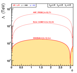
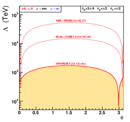
Figure 4: Reach as a function of the angle $\phi$ for different contributions of the dipole operator: (left) $\theta_{D}=\pi/2$, (middle) $\theta_{D}=\pi/4$, and (right) $\theta_{D}=3\pi/4$. Note that $\phi$ runs from $0\to 2\pi$, although it is plotted from $0\to\pi$; the rates for $\phi\in(\pi\to 2\pi)$ with positive dipole are equal to those with negative dipole and $\phi\in(0\to\pi)$. The solid region is currently excluded.

Finally, the dependence of the sensitivity on the angle $\phi$ and the variable $\kappa_{D}$ is exhibited in Figure 5. As expected, the $\mu\to e\gamma$ and $\mu\to e\bar{e}e$ processes are independent of $\phi$. The shape of the conversion processes on light and heavy targets are globally similar, although the ridges along which the rates cancel are slightly different.

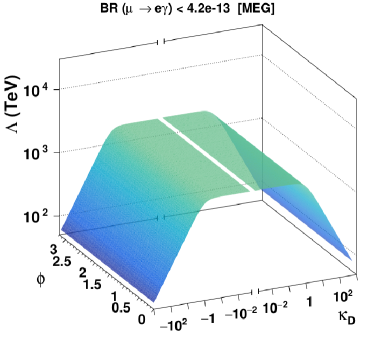
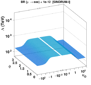
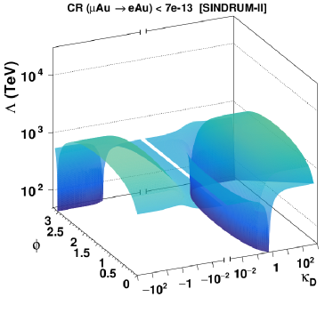
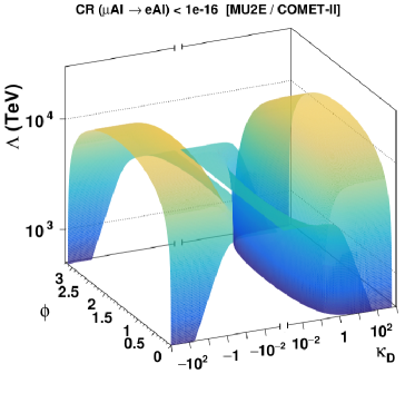
Figure 5: Reach as a function of the angle $\phi$ and the variable $\kappa_{D}$ for $\theta_{V}=\pi/4$ and $\theta_{S}=\pi/2$. Note that $\phi$ runs from $0\to 2\pi$, although it is plotted from $0\to\pi$; the rates for $\phi\in(\pi\to 2\pi)$ with positive dipole are equal to those with negative dipole and $\phi\in(0\to\pi)$.

IV Are scalar quark currents indistinguishable?

This section is somewhat independent of the rest of the paper, being focused on the information loss that occurs in matching nucleons to quarks at 2 GeV. In the data, LFV scalar interactions with neutrons might be distinguishable from those on protons DKY . But current theoretical translations of the nucleon results to quarks erase any distinction between LFV interactions with scalar $u$ or $d$ currents (the subdominant $s,c,b,t$ quarks are neglected in this section).

The Spin-Independent Conversion Rate (CR) is given in eqn (A.8) in terms of operator coefficients on nucleons. This result is at “Leading Order” in the low energy theory, and does not include the next order in $\chi$PT (parametrically $\sim 10$%, two-nucleon effects, pion exchange…) or in the nuclear matrix element. Such effects have been calculated for WIMP scattering Hetal , and some partial results for $\mu A\!\to\!eA$ have been obtained VCetal ; Dekens . Improvements of the theoretical calculation of $\Gamma(\mu A\!\to\!eA)$ could change the form of the conversion ratio (this occurs in VCetal ), or reduce the uncertainties on its parameters, thereby resolving the issue discussed here.

To set the stage, recall from KKO KKO that the overlap integrals for scalar and vector densities of neutrons and protons differ by less than a factor of three. In particular, Al approximately probes

$$C^{pp}_{S,R}+C^{pp}_{V,L}+C^{nn}_{S,R}+C^{nn}_{V,L}~{}~{},$$ (IV.1)

(neglecting the dipole which could be constrained/measured elsewhere). In addition, it was pointed out in DKY that measuring $\mu A\!\to\!eA$ on another light target with different numbers of $n$ and $p$ would allow the measurement of

$$C^{pp}_{S,R}+C^{pp}_{V,L}-C^{nn}_{S,R}-C^{nn}_{V,L}~{}~{}.$$ (IV.2)

Then, as noted by KKO, vector overlap integrals dominate over the scalars in heavy targets, so comparing Al to Au could allow to determine

$$C^{pp}_{S,R}-C^{pp}_{V,L}+C^{nn}_{S,R}-C^{nn}_{V,L}~{}~{}.$$ (IV.3)

However, heavy targets also have more neutrons, so the $n-p$ measurement from comparing two light targets is required to extract the $S-V$ from heavy targets. The one remaining combination of coefficients (an isospin-violating $V$-$S$ difference) has little impact on the CR given in eqn (A.8), and cannot be extracted with current theoretical uncertainties DKY .

$G^{p,u}_{V}=G^{n,d}_{V}=2$	$G^{p,d}_{V}=G^{n,u}_{V}=1$	$G^{p,s}_{V}=G^{n,s}_{V}=0$
$G^{p,u}_{S}=\frac{m_{p}}{m_{u}}0.0139(13)(12)=5.9$	$G^{p,d}_{S}=\frac{m_{p}}{m_{d}}0.0253(28)(24)=5.0$	$G^{p,s}_{S}=\frac{m_{N}}{m_{s}}0.043(11)=0.42$
$[G^{p,u}_{S}=\frac{m_{p}}{m_{u}}0.021(2)=9.0]$	$[G^{p,d}_{S}=\frac{m_{p}}{m_{d}}0.041(3)=8.2]$
$G^{n,u}_{S}=\frac{m_{n}}{m_{u}}0.0116(13)(11)=5.0$	$G^{n,d}_{S}=\frac{m_{n}}{m_{d}}0.0302(3)=6.0$	$G^{n,s}_{S}=\frac{m_{N}}{m_{s}}0.043(11)=0.42$
$[G^{n,u}_{S}=\frac{m_{n}}{m_{u}}0.019(2)=8.1]$	$[G^{n,d}_{S}=\frac{m_{n}}{m_{d}}0.045(3)=9.0]$
		$G^{N,c}_{S}=0.0543(=\frac{2m_{N}}{27m_{c}}f_{GG}^{N})$
		$G^{N,b}_{S}=0.0158(=\frac{2m_{N}}{27m_{b}}f_{GG}^{N})$

Table 3: Expectation values of vector and scalar quark currents in the nucleon; the scalar values are commonly called $f^{N}_{q}$ LLF , or for light quarks $\sigma_{\pi N}$ Hoferichter:2015dsa , where $G_{S}^{N,q}=\frac{m_{N}}{m_{q}}f^{N}_{q}=\sigma_{\pi N}/m_{q}$. The first scalar $G_{S}$ induced by light quarks are from the lattice Lellouch , and an average of lattice results  Junnarkar:2013ac is used for the strange quark. The second $G^{N,q}_{S}$ [in brackets] were obtained via EFT methods Hoferichter:2015dsa ; Alarcon:2011zs . The heavy quark scalar $G_{S}$s are from the lattice LLF , and in parentheses from  SVZ . In all cases, the $\overline{\rm MS}$ quark masses at $\mu=2$ GeV are taken as $m_{u}=2.2$ MeV, $m_{d}=4.7$ MeV, and $m_{s}=96$ MeV  Agashe:2014kda . The running heavy quark masses are PDB $m_{c}(m_{c})=1.27$ GeV, $m_{b}(m_{b})=4.18$ GeV. The nucleon masses are $m_{p}=938~{}{\rm MeV}$ and $m_{n}=939.6~{}{\rm MeV}$.

The operator coefficients on nucleons can be transformed to coefficients on quarks according to eqn (A.10), using the matrix $G$ given in Table 3. Focusing on the first generation valence quarks, this can be written as:

$$\left(\begin{array}[]{c}C^{pp}_{V,L}\\ C^{nn}_{V,L}\\ C^{pp}_{S,R}\\ C^{nn}_{S,R}\end{array}\right)=\left[\begin{array}[]{cccc}2&1&0&0\\ 1&2&0&0\\ 0&0&G_{S}^{pu}&G_{S}^{pd}\\ 0&0&G_{S}^{nu}&G_{S}^{nd}\end{array}\right]\left(\begin{array}[]{c}C^{uu}_{V,L}\\ C^{dd}_{V,L}\\ C^{uu}_{S,R}\\ C^{dd}_{S,R}\end{array}\right)$$ (IV.4)

where the vector coefficients exhibit the expected dominance of $u$ quarks in the proton, and $d$ quarks in the neutron: the quark vector coefficients can be calculated from the nucleon vector nucleon coefficients, and vice versa. In the case of the scalar coefficients, this is almost not the case; for both lattice and EFT determinations of the $G_{S}^{N,q}$, the determinant of the scalar submatrix in eqn (IV.4) is small compared to the product of two $G_{S}^{N,q}$ ($G_{S}^{pu}G_{S}^{nd}-G_{S}^{pd}G_{S}^{nu}$ $\sim 9^{2}-8^{2}(6^{2}-5^{2})$), causing large uncertainties when it is inverted to solve for quark coefficients as a function of nucleon coefficients. In addition, $G_{S}^{N,q}\gg G_{V}^{N,q}$ increases the sensitivity to scalar coefficients, and reduces the relative contribution of the vector coefficients to about the magnitude of the scalar uncertainties.

The effects of transforming from nucleon operators to quark operators can be seen in Figure 6, where are plotted the quark and nucleon overlap integrals. This illustrates the difficulty to distinguish scalar $u$ vs $d$, and also that the variation with $Z$ is reduced for the quarks compared to nucleons.

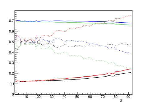
Figure 6: Normalised quark (solid) and nucleon (dotted) overlap integrals as a function of the target charge $Z$. From the top-down at $Z=$ 90: vector $n$ (red, dotted), scalar $d$ (blue) and $u$ (green), vector $p$ (black,dotted), scalar $n$ (blue,dotted) and $p$ (green, dotted), and vector $d$ (red) and $u$ (black). The overlap integrals for given $Z$ are normalised by dividing by the thesquare root of the sum of the squared integrals.

The ability of different targets to distinguish among operator coefficients can be quantified as the angle between the directions they probe in coefficient space DKY , where the direction is given by the overlap integrals for the target. Figure 7 plots this misalignment angle as a function of $Z$ for various past and future targets. The plot on the left is for quark coefficients, and on the right is for nucleon coefficients (notice the difference in the vertical scale). Reference DKY estimated that a misalignment angle $\mathrel{\vbox{\hbox{$>$}\nointerlineskip\hbox{$\sim$}}}0.1$ was required to overcome theoretical uncertainties in the nuclear calculation, and obtain independent measurement of distinct nucleon operator coefficients. Even if one neglects the theoretical uncertainty in the $G_{O}^{N,q}$s, applying this $\mathrel{\vbox{\hbox{$>$}\nointerlineskip\hbox{$\sim$}}}0.1$ rule for quark coefficients suggests that the theoretical accuracy needs to be improved.

In summary, upcoming experiments could hope to bound or measure the three combinations of nucleon coefficients given in eqns (IV.1-IV.3). However, due to the almost-vanishing scalar determinant in eqn (IV.4), theoretical progress in calculating the $G^{Nq}_{S}$ is required, for these to constrain three independent combinations of quark operator coefficients.

Figure 7: Misalignement angle between target vectors, calculated for quarks and nucleons. Notice the reduced vertical scale and smoother lines in the quark plot. The decreasing lines are lead (green,upper) and Au (blue); the rising lines are titanium (blue) and Al (red,dashed, middle) and lithium (black,dashed, upper).

V Summary

We use bottom-up EFT to calculate the reach and illustrate the complementarity of experiments searching for NP. This method is particularly well-suited to situations in which the number of observables is much smaller than the number of operators. It provides a complete parametrisation of the rates, without redundancies, and the EFT translation to $\Lambda_{LFV}$ can be systematically improved. In addition, this formalism allows to explore the complementarity in a self-consistent manner at the same scale at which the theory is defined, and ensure that experiments effectively probe different combinations of NP parameters. This approach is generic and can be applied to many situations. In this manuscript, we use it to study CLFV in the muon sector and derive sensitivity projections for current and future experiments.

At the experimental scale, the Lagrangian given in eqn (II.1) includes all and only the operators contributing at tree level to the observables. The combinations of coefficients constrained experimentally define the operator basis for our subspace, whose dimension is equal to the number of constraints. For $\mu\to e_{L}\gamma$, $\mu\to e_{L}\bar{e}e$ and Spin Independent $\mu{\rm Al}\to e_{L}{\rm Al}$ and $\mu{\rm Au}\to e_{L}{\rm Au}$, this subspace is six-dimensional. These coefficients are translated to $\Lambda_{NP}$ by solving the leading order Renormalisation Group Equations below the weak scale, and matching them to SMEFT at tree level (see eqn (II.7)). Since the number of constraints remains unchanged, the dimension of the subspace cannot grow (but it could decrease, as discussed in section IV). However, the normalisation and direction of the basis vectors is altered, in order to include, at $\Lambda_{LFV}$, the contributions from all the operators to the observables via short-distance effects described in the RGEs.

The ability of different experiments to probe independent operator coefficients – our definition of complementarity – is related to the misalignement between vector of coefficients. While it can be measured in various ways, we observe that a judiciously selected subset of our basis vectors remain approximately orthogonal above the weak scale, and we use various parametrisations (see table 2 or eqn (III.1)) to plot the experimental exclusion curves using the Branching Ratios given in eqn (B.3). We also display a few projections to illustrate the reach and complementarity of future experiments.

An example of distinct observables probing the same New Physics is recalled in section IV: $\mu A\!\to\!eA$ on various nuclei could distinguish scalar $\mu\to e$ contact interactions on neutrons from protons, but this may not allow the distinction of LFV scalar operators involving up quarks from those with down quarks. Improving the precision of the scalar $\bar{q}q$ expectation values in the nucleon would be required to improve the situation.

This work is only a preliminary implementation of bottom-up EFT, relying on theoretical formalism described in C+C . In future work, we aim to implement the Renormalisation Group running of our vectors above the weak scale (it was neglected here for simplicity and the lack of knowledge of $\Lambda_{LFV}$), and match models onto the “observable subspace” at $\Lambda_{LFV}$. We hope that finding robust distinctions among model predictions could be simplified by the reduced dimension of the subspace.

Acknowledgements

SD thanks A Ibarra for a seminar invitation and discussions.

Appendix A Operators, Rates and R-matrices at low energy

The operators contributing at the experimental scale $\sim m_{\mu}$ to the tree level amplitudes for $\mu\to e_{L}\gamma$, $\mu\to e_{L}\bar{e}e$ and Spin Independent $\mu A\to e_{L}A$ are given in eqn (II.1), where the $\mu A\!\to\!eA$ operators can be expanded on:

$${\cal O}^{NN}_{S,R}=\overline{e}P_{R}\mu\overline{N}N ~{},~{} {\cal O}^{NN}_{V,L}=\overline{e}\gamma^{\alpha}P_{L}\mu\overline{N}\gamma_{\alpha}N$$ (A.1)

where $N\in\{p,n\}$, and the list neglects subdominant operators such as $\overline{e}P_{X}\mu FF$ DKUY .

The Branching Ratios (BRs) for the various processes can be expressed in terms of the operator coefficients $\vec{C}$ and the matrices R:

$$BR(\mu\to e_{L}\gamma) = \frac{v^{4}}{\Lambda_{LFV}^{4}}\vec{C}^{\dagger}\bm{R}_{\mu\to e_{L}\gamma}\vec{C}$$ (A.2)

$$\Leftrightarrow \bm{R}_{\mu\to e_{L}\gamma}(m_{\mu})=384\pi^{2}\frac{v^{4}}{\Lambda_{LFV}^{4}}\hat{e}_{D}\hat{e}^{\dagger}_{D}$$

where $v\simeq m_{t}$ is the Higgs vev, and $\vec{C}\cdot\hat{e}_{D}={C}_{D}$. For $\mu\to e_{L}\bar{e}e$, the BRs given in the text can be written using:

$$\bm{R}_{\mu\to e_{L}\bar{e}e}(m_{\mu}) = \frac{v^{4}}{\Lambda_{LFV}^{4}}\left[\begin{array}[]{cccc}2&0&0&8e\\ 0&1&0&4e\\ 0&0&\frac{1}{8}&0\\ 8e&4e&0&8e^{2}(8\ln\frac{m_{\mu}}{m_{e}}-11)\\ \end{array}\right]$$ (A.7)

where R is given in the basis $(C^{e\mu ee}_{VL},C^{e\mu ee}_{VR},C^{e\mu ee}_{S},C^{e\mu ee}_{D})$.

For $\mu A\!\to\!eA$, we consider the conversion ratios on prototypical heavy and light targets, taken to be Au and Al. Following Kitano, Koike and Okada (KKO) KKO , the Spin-Independent conversion rate can be written

$${\rm CR}_{SI}(\mu A\to e_{L}A) = \frac{4m_{\mu}^{5}}{\Lambda_{LFV}^{4}\Gamma_{capt}}\big{|}{C}^{pp}_{V,L}V_{A}^{(p)}+{C}^{pp}_{S,R}S_{A}^{(p)}+{C}^{nn}_{V,L}V_{A}^{(n)}+{C}^{nn}_{S,R}S_{A}^{(n)}+C_{D,R}{\frac{D_{A}}{4}}\big{|}^{2}$$ (A.8)

where we use the nucleus($A$)- and nucleon($N$)-dependent “overlap integrals” $V_{A}^{(N)}$, $S_{A}^{(N)}$, $D_{A}$ given by KKO KKO , and $\Gamma_{cap}$ is the rate for the muon to transform to a neutrino by capture on the nucleus. Some relevant rates are Suzuki:1987jf :

$$\Gamma_{capt}=g_{A}^{cap}\times 10^{6}{\rm sec}^{-1}=\left\{\begin{array}[]{cc}Al&0.7054\\ Ti&2.59\\ Au&13.07\end{array}\right\}\times 10^{6}{\rm sec}^{-1}$$ (A.9)

KKO observed that the overlap integrals were nucleus-dependent, and measurements of $\mu\!\to\!e~{}{\rm conversion}$ on different targets could be used to determine the operator coefficients. Reference DKY explored this issue quantitatively, and showed that with current uncertainties, Ti and Au give independent constraints. In this work, we are interested in a slightly different question: whether the observables give different constraints on New Physics heavier than $m_{\mu}$ and $\Lambda_{QCD}$, instead of understanding if they are independent. Unfortunately, there is “information loss” in matching nucleons onto quarks (see section IV), so we match the nucleon onto quark operators before constructing the R-matrices for $\mu{\rm Al}\to e_{L}{\rm Al}$ and $\mu{\rm Au}\to e_{L}{\rm Au}$.

Nucleon operators can be matched at 2 GeV onto light quark operators (see C+C for a basis) as

$$\langle N(P_{f})|\bar{q}(x)\Gamma_{O}q(x)|N(P_{i})\rangle\simeq G^{N,q}_{O}\langle N(P_{f})|\bar{N}(x)\Gamma_{O}N(x)|N(P_{i})\rangle=G^{N,q}_{O}\overline{u_{N}}(P_{f})\Gamma_{O}u_{N}(P_{i})e^{-i(P_{f}-P_{i})x}~{}~{}~{}.$$

We also include the two-step matching of scalar $b$ and $c$ operators $(\bar{e}P_{R}\mu)(\bar{Q}Q)$ SVZ ; CKOT , first onto the gluon operator $(\bar{e}P_{R}\mu)GG$, then onto nucleons. As a result, the nucleon and quark coefficients are related as

$${C}^{NN}_{O,X}=\sum_{q}G_{O}^{Nq}C_{O,X}^{qq}~{}~{}~{},$$ (A.10)

where $O\in\{S,V\}$ and the relevant $G$s are given in Table 3. One can then define quark “overlap integrals” for target $A$ as

$$I^{q}_{A,S} = G_{S}^{pq}S_{A}^{p}+G_{S}^{nq}S_{A}^{n}$$

$$I^{q}_{A,V} = G_{V}^{pq}V_{A}^{p}+G_{V}^{nq}V_{A}^{n}$$ (A.11)

where in this work we use the EFT results Hoferichter:2015dsa for $G_{S}^{N,q}$, which differ by $\sim$50% from lattice results Lellouch ; LLF . Assembling the quark overlap integrals for target $A$ into a “target vector” $\vec{u}_{A}$:

$$\vec{u}_{A} = (I^{b}_{A,S},I^{c}_{A,S},I^{s}_{A,S},I^{u}_{A,S},I^{d}_{A,S},I^{u}_{A,V},I^{d}_{A,V})~{}~{},$$ (A.12)

allows to write the Conversion Ratio as

$${\rm CR}_{SI}(\mu A\to e_{L}A) = \frac{6144\pi^{3}v^{4}}{2.197g^{cap}_{A}\Lambda_{LFV}^{4}}\left|\vec{u}_{A}\cdot\vec{C}+C_{D}\frac{D_{A}}{4}\right|^{2}$$ (A.13)

$$\equiv \vec{C}^{\dagger}\bm{R}_{\mu A\to e_{L}A}\vec{C}$$

where $D_{A}$ is the KKO overlap integrals for the dipole KKO . So theR-matrix at a scale of 2 GeV is

$$\bm{R}_{\mu A\to e_{L}A} = \frac{6144\pi^{3}v^{4}}{2.197g^{cap}_{A}\Lambda_{LFV}^{4}}{\Big{(}}\vec{u}_{A}+\frac{D_{A}}{4}\hat{e}_{D}{\Big{)}}\otimes{\Big{(}}\vec{u}_{A}+\frac{D_{A}}{4}\hat{e}_{D}{\Big{)}}^{\dagger}$$ (A.14)

This translation of nucleon to quark operators neglects higher order QED and “strong interaction” effects between the experimental scale $m_{\mu}$ and 2 GeV: the QED running is small for the considered operators, and we did not include recent $\chi$PT results  VCetal . The prospects of distinguishing coefficients by using different targets depend on the misalignment between the target vectors. In the quark operator basis at 2 GeV, this angle is given for various potential targets in Table 4. The angles are smaller than the misalignmeent angles in the nucleon operator basis (see Figure 7), because the scalar quark overlap integrals are larger than the vector integrals, and comparable for $u$ and $d$ quarks. In addition, there is currently a large discrepancy, $\sim 50$%, between lattice and EFT determinations of the scalar overlap integrals. We assume that this theoretical discrepancy can be solved, so that $\mu A\to e_{L}A$ on Au and Al give independent information.

$\begin{array}[]{|c|cccccc|}\hline\cr&{\rm Li}&{\rm Al}&{\rm Ti}&{\rm Cu}&{\rm Au}&{\rm Pb}\\ \hline\cr{\rm Li}&-&0.545&0.714&1.06&5.57&6.69\\ {\rm Al}&&-&0.433&0.760&5.34&6.46\\ {\rm Ti}&&&-&0.356&4.94&6.06\\ {\rm Cu}&&&&-&4.59&5.71\\ {\rm Au}&&&&&-&1.12\\ \hline\cr\end{array}$

Table 4: Misalignment angles (in degrees), between target vectors expressed in the quark operator basis.

Eqn (A.14) gives the R-matrices for Al and Au, which probe directions in quark coefficient space that are misaligned by $\sim$ 5 degrees, at a scale of 2 GeV. In the plane spanned by $\vec{u}_{Au}$ and $\vec{u}_{Al}$, the orthogonal combinations used in eqn (II.1), can be obtained by writing the target vector $\vec{u}_{Au}$ for Au as:

$$\vec{u}_{Au}=|\vec{u}_{Au}|(\cos\theta_{\rm AuAl}\hat{u}_{Al}+\sin\theta_{\rm AuAl}\hat{u}_{\perp})\Rightarrow\hat{u}_{\perp}=\frac{\hat{u}_{Au}-\cos\theta_{AuAl}\hat{u}_{Al}}{\sin\theta_{AuAl}}~{}~{}~{}~{}~{}~{}~{}~{}~{}~{}~{}~{}~{}~{}~{}~{}~{}~{}~{}~{}~{}~{}~{}~{}$$

where $\theta_{AuAl}$ is given in Table 4, and $\vec{u}_{\perp}\approx.56C^{uu}_{V}+.8C^{dd}_{V}$ is the direction in coefficient space corresponding to the operator ${\cal O}_{Aheavy\perp}$ of eqn (II.1).

Appendix B Including the penguin

This Appendix discusses the orthogonality of the basis used for the experimentally accessible subspace. We need an orthogonal basis to illustrate complementarity in polar coordinates; orthogonality would not be required to evaluate complementarity via eqn (II.6), nor for exploring the model predictions for coefficients in the subspace. In the following, the term “penguins” refer to the operators of eqn (B.1).

The basis vectors at $\Lambda_{LFV}\mathrel{\vbox{\hbox{$>$}\nointerlineskip\hbox{$\sim$}}}m_{W}$ are G${}^{*}(m_{W},m_{\mu})\hat{e}_{A}$; we do not give explicit expressions because the translation from the observable-motivated basis to an arbitrary other choice is a technicality more suitable to computers. Expressions for various $\vec{C}^{\dagger}\bm{G}^{*}(m_{W},m_{\mu})\hat{e}_{A}$, appropriate for calculating LFV BRs in terms of coefficients at the weak scale, can be found in C+C . The norms and inner products among some basis vectors are given in Table 5, which shows an overlap of $10\to 20$ degrees between the vector operators ($e_{\perp}$ has significant quark-vector components). The shrinking of the quark target-vectors is largely due to the shrinking scalar coefficients.

The overlap among the coefficients of $(\bar{e}\gamma^{\alpha}P_{L}\mu)(\bar{f}\gamma_{\alpha}f)$ operators arises because the $\mu\to e$ penguin operators of the SM EFT  polonais :

$$\delta{\cal L}_{penguin}=\frac{C_{HL1}}{\Lambda_{LFV}^{2}}(\overline{\ell}_{e}\gamma^{\alpha}\ell_{\mu})(H^{\dagger}\stackrel{{\scriptstyle\leftrightarrow}}{{D_{\alpha}}}H)+\frac{C_{HL3}}{\Lambda_{LFV}^{2}}(\overline{\ell}_{e}\tau^{a}\gamma^{\alpha}\ell_{\mu})(H^{\dagger}\stackrel{{\scriptstyle\leftrightarrow}}{{D^{a}_{\alpha}}}H)$$ (B.1)

generate a flavour-changing vertex $\frac{gv^{2}}{c_{W}\Lambda_{LFV}^{2}}(C^{e\mu}_{HL1}+C^{e\mu}_{HL3})\bar{e}\,Z\!\!\!\!/~{}P_{L}\mu$, so that $Z$ exchange gives four-fermion operators in the low energy EFT:

$$\delta{\cal L}=\sum_{f,X}\frac{g^{f}_{X}(C^{e\mu}_{HL1}+C^{e\mu}_{HL3})}{\Lambda_{LFV}^{2}}(\overline{e}\gamma^{\alpha}P_{L}\mu)(\overline{f}\gamma^{\alpha}P_{X}f)$$ (B.2)

where $f$ is any light chiral fermion, we used the SM $Z$ interaction $\frac{g}{2c_{W}}(g^{f}_{L}P_{L}+g^{f}_{R}P_{R})$ and $c_{W}=\cos\theta_{W}$. As a result, at the weak scale, the basis vectors $\vec{e}_{VL}$ and $\vec{e}_{VR}$ have components $g^{e}_{L}$ and $g^{e}_{R}$ in the two penguin directions, respectively, giving a tree-level contribution to $\vec{e}_{VL}\cdot\vec{e}_{VR}$ of order $2g^{e}_{L}g^{e}_{R}=4s_{W}^{2}(-1+2s_{W}^{2})$.

A more orthogonal basis could be obtained by removing the penguin contribution from the low energy $(\bar{e}\gamma^{\alpha}P_{L}\mu)(\bar{f}\gamma_{\alpha}f)$ operators, and adding $Z\to\mu e_{L}$ as an observable at $m_{W}$. This is analogous to what was already done for the dipole, removing it from the combination of operators contributing to $\mu A\!\to\!eA$, and including $\mu\to e\gamma$ as an observable. However, this adds a dimension to the subspace, and tangles the intuitive link between basis vectors and observables. It is pursued in section B.2. Section B.1 describes a simpler approach used to make the plots in the body of the paper.

$\begin{array}[]{|c|cccccc|}\hline\cr&\vec{e}_{Alight}&\vec{e}_{Aheavy\perp}&\vec{e}_{VL}&\vec{e}_{VR}&\vec{e}_{S}&\vec{e}_{D}\\ \hline\cr\vec{e}_{Alight}&0.768&{.05}&0.022&-0.018&0&0\\ \vec{e}_{Aheavy\perp}&&0.891&\bm{0.16}&\bm{-0.14}&0&0\\ \vec{e}_{VL}&&&1.13&\bm{-0.354}&0&0\\ \vec{e}_{VR}&&&&1.29&0&0\\ \vec{e}_{S}&&&&&1.00&0\\ \vec{e}_{D}&&&&&&1.39\\ \hline\cr\end{array}$

Table 5: Inner products between the basis vectors $\vec{e}_{i}(\Lambda_{LFV}\sim m_{W})=\bm{G}^{*}(m_{W},m_{\mu})\hat{e}_{i}$. On the diagonal are the norms (at $m_{W}$ in SMEFT, for unit-normalised $\hat{e}_{i}$ at low energy), whereas the off-diagonals are $\cos\eta$, where $\eta$ is the angle between the vectors. Overlaps smaller than $10^{-3}$ are given as 0.

B.1 A reduced basis at $\Lambda_{LFV}\sim m_{W}$

In this section we outline a method for choosing a penguin-less basis vector corresponding to a linear combination of $\vec{e}_{VL}$ and $\vec{e}_{VR}$, which is approximately orthogonal to the remaining basis vectors. In addition, the complementarity plots involving $\vec{e}_{VL}$ or $\vec{e}_{VR}$ are similar, so this choice suppresses redundancy.

The dependence of BR($\mu\to e\bar{e}e$) on $C_{VL}$ and $C_{VR}$ is very similar, as can be seen from eqn (II.3). Since these coefficients can be distinguished via the angular distributions of the final state electrons in $\mu\to e\bar{e}e$ Okadameee rather than by comparing BR($\mu\to e\gamma$) and BR($\mu\to e\bar{e}e$), it is sufficient to plot $\mu\to e\gamma$ and $\mu\to e\bar{e}e$ in terms of a combination of these coefficients. By choosing this combination to suppress penguin contribution, we obtain five approximately orthogonal basis vectors.

As mentioned above, in the SMEFT basis at $m_{W}$, $\vec{e}_{VL}$ and $\vec{e}_{VR}$ have components $\sim g^{e}_{L},g^{e}_{R}$ along the directions of the penguin operators of eqn (B.1). So introducing $\vec{e}_{V}\propto g^{e}_{R}\vec{e}_{VL}-g^{e}_{L}\vec{e}_{VR}$, one sees that its penguin component vanishes at tree level, and $\vec{e}_{V}$ will be orthogonal to $\vec{e}_{Aheavy\perp}$ up to loop effects. We therefore replace the $\vec{e}_{VR}\otimes\vec{e}_{VL}$ plane by an axis along $\vec{e}_{V}$ and plot the complementarity of the three rates in the resulting 5-dimensional space.

In this reduced basis, the BRs can be written in terms of operator coefficients at $\Lambda_{LFV}\sim m_{W}$ as

$${\rm BR}(\mu\to e_{L}\gamma) = 384\pi^{2}\frac{v^{4}}{\Lambda_{LFV}^{4}}\left[|\vec{e}_{D}|\cos\theta_{D}\right]^{2}$$

$${\rm BR}(\mu\to e\bar{e}e) = \frac{v^{4}}{\Lambda_{LFV}^{4}}{\Big{[}}\frac{|\vec{e}_{S}|^{2}\sin^{2}\theta_{D}\cos^{2}\theta_{S}}{8}+(|\vec{e}^{~{}^{\prime}}_{VR}|\sin\theta_{D}\sin\theta_{S}\cos\theta_{V}+4e|\vec{e}_{D}|\cos\theta_{D})^{2}$$

$$+2(|\vec{e}^{~{}^{\prime}}_{VL}|\sin\theta_{D}\sin\theta_{S}\cos\theta_{V}+4e|\vec{e}_{D}|\cos\theta_{D})^{2}+18.76(|\vec{e}_{D}|\cos\theta_{D})^{2}{\Big{]}}$$

$${\rm BR}(\mu Al\to eAl) = \frac{6144\pi^{3}v^{4}}{2.197g^{cap}_{Al}\Lambda_{LFV}^{4}}{\Big{[}}|\vec{u}_{Al}||\vec{e}_{Al}|\sin\theta_{D}\sin\theta_{S}\sin\theta_{V}\sin\phi+\frac{D_{Al}}{4}|\vec{e}_{D}|\cos\theta_{D}{\Big{]}}^{2}$$

$${\rm BR}(\mu Au\to eAu) = \frac{6144\pi^{3}v^{4}}{2.197g^{cap}_{Au}\Lambda_{LFV}^{4}}{\Big{[}}|\vec{u}_{Au}|(\cos\theta_{AuAl}|\vec{e}_{Al}|\sin\theta_{D}\sin\theta_{S}\sin\theta_{V}\sin\phi$$ (B.3)

$$+\sin\theta_{AuAl}|\vec{e}_{\perp}|\sin\theta_{D}\sin\theta_{S}\sin\theta_{V}\cos\phi)+\frac{D_{Au}}{4}|\vec{e}_{D}|\cos\theta_{D}{\Big{]}}^{2}$$

where we replace $\{\theta_{VR},\theta_{VL}\}\to\theta_{V}$, the un-primed norms of the basis vectors at $m_{W}$ are on the diagonal of Table 5 and $|\vec{e}^{~{}^{\prime}}_{VR}|=-g^{e}_{L}|\vec{e}_{VR}|/\sqrt{(g^{e}_{L})^{2}+(g^{e}_{R})^{2}}=1.05$, $|\vec{e}^{~{}^{\prime}}_{VL}|=g^{e}_{L}|\vec{e}_{VL}|/\sqrt{(g^{e}_{R})^{2}+(g^{e}_{R})^{2}}=0.709$, $\theta_{\rm AuAl}$ is in Table 4, and norms obtained from the $\mu A\!\to\!eA$ overlap integrals and nucleon-quark matching are $|\vec{u}_{Al}|=0.39706$ $|\vec{u}_{Ti}|=0.991275$, and $|\vec{u}_{Au}|=1.92876$.

B.2 An enlarged basis at $\Lambda_{LFV}\sim m_{W}$

This section outlines the approach of adding $Z\to e^{\pm}\mu^{\mp}$ to the observables, and removing the contribution of the flavour-changing $Z$ penguin from the four-fermion operators. This ensures that the basis vectors are orthogonal at $m_{W}$ to within a degree or two, and highlights the importance of $Z\to e^{\pm}\mu^{\mp}$ for distinguishing among coefficients and models.

The operators ${\cal O}^{e\mu}_{HL1}$ and ${\cal O}^{e\mu}_{HL3}$ of eqn (B.1) mediate flavour-changing $Z$ decays, upon which ATLAS  ATLASZmue sets the constraint $BR(Z\to e^{\pm}\mu^{\mp})<7.5\times 10^{-7}$ (based on 20 fb^-1 of luminosity), implying:

$$\frac{v^{2}}{\Lambda_{LFV}^{2}}|C^{e\mu}_{HL1}+C^{e\mu}_{HL3}|\mathrel{\vbox{\hbox{$<$}\nointerlineskip\hbox{$\sim$}}}1.6\times 10^{-3}$$ (B.4)

The current sensitivity of $\mu A\!\to\!eA$ and $\mu\to e\bar{e}e$ to these coefficients is three orders of magnitude better, and should improve by another two orders of magnitude with upcoming experiments. Nonetheless, improving the experimental reach in $Z\to e^{\pm}\mu^{\mp}$ is interesting, because experiments at muon mass scale cannot distinguish these penguin operators from the four-fermion ones

We include an additional basis vector in the coefficient subspace above $m_{W}$ :

$$\hat{e}_{ping}=\frac{1}{\sqrt{2}}(\hat{e}_{HL1}+\hat{e}_{HL3)}$$ (B.5)

(for the case of an outgoing $e_{L}$; for outgoing $e_{R}$ it would be $\hat{e}_{HE}$), and rewrite the operator coefficients in spherical coordinates as

$$\vec{C} = \frac{1}{\Lambda_{LFV}^{2}}{\Big{[}}\cos\theta_{ping}\hat{e}_{ping}+\sin\theta_{ping}\cos\theta_{D}\hat{e}_{D}+\sin\theta_{ping}\sin\theta_{D}\cos\theta_{S}\hat{e}_{S,R}+\sin\theta_{ping}\sin\theta_{D}\sin\theta_{S}\cos\theta_{VR}\hat{e}_{V,R}$$ (B.6)

$$+\sin\theta_{ping}\sin\theta_{D}\sin\theta_{S}\sin\theta_{VR}\cos\theta_{VL}\hat{e}_{V,L}+\sin\theta_{ping}\sin\theta_{D}\sin\theta_{S}\sin\theta_{VR}\sin\theta_{VL}(\sin\phi\hat{e}_{Al}+\cos\phi\hat{e}_{\perp}){\Big{]}}~{}~{}~{}~{},~{}~{}~{}~{}$$

where $\theta_{J}:0..\pi$ and $\phi:0..2\pi$, and recall that a model would predict the various angles and the scale.

The expressions for low energy BRs in this enlarged basis become more complicated, because the low energy four-fermion coefficients are expressed as the component from $Z$ exchange, plus the component from four-fermion operator at the weak scale. The normalisation of some basis vectors changes as well, becoming:

$$|e_{VL}|=0.944~{},~{}|e_{VR}|=1.041~{},~{}|e_{Al}|=0.768~{},~{}|e_{Aheavy\perp}|=0.861$$ (B.7)

The formulae for the reach, obtained from the Branching Ratios are:

$$\frac{\Lambda}{v} = \left[\frac{384\pi^{2}}{{\rm BR}(\mu\to e_{L}\gamma)}\right]^{1/4}\sqrt{(|\vec{e}_{D}|\sin\theta_{ping}\cos\theta_{D}+1.21\times 10^{-3}\cos\theta_{ping})^{2}}$$ (B.8)

where the one-loop matching of penguin operators to the dipole was included. For $\mu\to e\bar{e}e$:

$$\frac{\Lambda}{v} = \left[\frac{1}{{\rm BR}(\mu\to e\bar{e}e)}\right]^{1/4}\sqrt{\frac{|\vec{e}_{S}|\sin\theta_{ping}\sin\theta_{D}\cos\theta_{S}}{2\sqrt{2}}}$$

$$\frac{\Lambda}{v} = \left[\frac{1}{{\rm BR}(\mu\to e\bar{e}e)}\right]^{1/4}{\Big{[}}(|\vec{e}_{VR}|\sin\theta_{ping}\sin\theta_{D}\sin\theta_{S}\cos\theta_{VR}+0.685\cos\theta_{ping}+4e|\vec{e}_{D}|\sin\theta_{ping}\cos\theta_{D})^{2}$$

$$+9.38(|\vec{e}_{D}|\sin\theta_{ping}\cos\theta_{D})^{2}{\Big{]}}^{1/4}$$

$$\frac{\Lambda}{v} = \left[\frac{1}{{\rm BR}(\mu\to e\bar{e}e)}\right]^{1/4}{\Big{[}}2(|\vec{e}_{VL}|\sin\theta_{ping}\sin\theta_{D}\sin\theta_{S}\sin\theta_{VR}\cos\theta_{VL}-0.722\cos\theta_{ping}+4e|\vec{e}_{D}|\sin\theta_{ping}\cos\theta_{D})^{2}$$ (B.9)

$$+9.38(|\vec{e}_{D}|\sin\theta_{ping}\cos\theta_{D})^{2}{\Big{]}}^{1/4}$$

where $0.685$ and -$0.722$ correspond respectively to $\sqrt{2}g^{e}_{R,L}\times$QED loop corrections. Finally, subtracting the penguins from the $u$ and $d$ vector operators in $\mu A\!\to\!eA$ gives

$$\frac{\Lambda}{v} = \left[\frac{1.2292\times 10^{5}}{{\rm BR}(\mu Al\to eAl)}\right]^{1/4}{\Big{[}}|\vec{u}_{Al}|(|\vec{e}_{Al}|\sin\theta_{ping}\sin\theta_{D}\sin\theta_{S}\sin\theta_{VR}\sin\theta_{VL}\sin\phi-0.0263\cos\theta_{ping})$$ (B.10)

$$+\frac{D_{Al}}{4}|\vec{e}_{D}|\sin\theta_{ping}\cos\theta_{D}{\Big{]}}^{1/2}$$

$$\frac{\Lambda}{v} = \left[\frac{6.63435\times 10^{3}}{{\rm BR}(\mu Au\to eAu)}\right]^{1/4}{\Big{[}}|\vec{u}_{Au}|(\cos\theta_{\rm AuAl}|\vec{e}_{Al}|\sin\theta_{ping}\sin\theta_{D}\sin\theta_{S}\sin\theta_{VR}\sin\theta_{VL}\sin\phi$$

$$+\sin\theta_{\rm AuAl}|\vec{e}_{\perp}|\sin\theta_{ping}\sin\theta_{D}\sin\theta_{S}\sin\theta_{VR}\sin\theta_{VL}\cos\phi-0.0474\cos\theta_{ping})+\frac{D_{Au}}{4}|\vec{e}_{D}|\sin\theta_{ping}\cos\theta_{D}{\Big{]}}^{1/2}$$

B.3 The eigenbasis of the covariance matrix

An alternative basis for the subspace of constrained coefficients, also orthogonal and perhaps more familiar, would be the eigenvectors of the covariance matrix. The inverse covariance matrix $\bm{V}$ for all the processes can be written as

$$\vec{C}^{\dagger}\bm{V}\vec{C} = \vec{C}^{\dagger}\frac{\bm{R}_{\mu\to e\gamma}}{B_{\mu\to e\gamma}^{expt}}\vec{C}+\vec{C}^{\dagger}\frac{\bm{R}_{\mu\to e\bar{e}e}}{B_{\mu\to e\bar{e}e}^{expt}}\vec{C}+\vec{C}^{\dagger}\frac{\bm{R}_{\mu{\rm Al}\to e{\rm Al}}}{B_{\mu{\rm Al}\to e{\rm Al}}^{expt}}\vec{C}+\vec{C}^{\dagger}\frac{\bm{R}_{\mu{\rm Au}\to e{\rm Au}}}{B_{\mu{\rm Au}\to e{\rm Au}}^{expt}}\vec{C}~{}~{},$$ (B.11)

where the coefficients are evaluated at the experimental scale. The inverse eigenvalues give the allowed range of coefficients in the eigenbasis, and the eigenvectors are orthogonal combinations of operators, which correspond to the axes of the allowed ellipse around the origin in coefficient space. This is a convenient basis for plotting, because the limiting values of each parameter are obtained on the axes, so there is no need to do perform scans. However, we prefer the operator basis of eqn (II.1), because it is simple and directly related to the experimental processes.

A covariance matrix for the coefficients at $\Lambda_{LFV}$ can be obtained by substituting eqn (II.7) into eqn (B.11). This matrix is large, ($\sim 90\times 90$), so despite that most of the eigenvalues should vanish, finding the eigenvectors of the 12 non-zero eigenvalues would be a numerical exercise which could disconnect the final basis and constraints from the input processes. It has the advantage of giving an orthonormal basis, whose eigenvectors correspond to the axes of the allowed ellipse in coefficient space.

References

- (1) Y. Kuno and Y. Okada, “Muon decay and physics beyond the standard model,” Rev. Mod. Phys. 73 (2001), 151-202 doi:10.1103/RevModPhys.73.151 [arXiv:hep-ph/9909265 [hep-ph]].
- (2) L. Calibbi and G. Signorelli, “Charged Lepton Flavour Violation: An Experimental and Theoretical Introduction,” Riv. Nuovo Cim. 41 (2018) no.2, 71-174 doi:10.1393/ncr/i2018-10144-0 [arXiv:1709.00294 [hep-ph]].
- (3) M. C. Gonzalez-Garcia and Y. Nir, “Neutrino Masses and Mixing: Evidence and Implications,” Rev. Mod. Phys. 75 (2003), 345-402 doi:10.1103/RevModPhys.75.345 [arXiv:hep-ph/0202058 [hep-ph]].
- (4) M. Fukugita and T. Yanagida, “Baryogenesis Without Grand Unification,” Phys. Lett. B 174 (1986), 45-47 doi:10.1016/0370-2693(86)91126-3
- (5) S. Davidson, E. Nardi and Y. Nir, “Leptogenesis,” Phys. Rept. 466 (2008), 105-177 doi:10.1016/j.physrep.2008.06.002 [arXiv:0802.2962 [hep-ph]].
- (6) A. M. Baldini et al. [MEG Collaboration], “Search for the lepton flavour violating decay with the full dataset of the MEG experiment,” Eur. Phys. J. C 76 (2016) no.8, 434 doi:10.1140/epjc/s10052-016-4271-x [arXiv:1605.05081 [hep-ex]].
- (7) A. M. Baldini et al. [MEG II Collaboration], “The design of the MEG II experiment,” Eur. Phys. J. C 78 (2018) no.5, 380 doi:10.1140/epjc/s10052-018-5845-6 [arXiv:1801.04688 [physics.ins-det]].
- (8) U. Bellgardt et al. [SINDRUM Collaboration], “Search for the Decay mu+ -> e+ e+ e-,” Nucl. Phys. B 299 (1988) 1. doi:10.1016/0550-3213(88)90462-2
- (9) A. Blondel et al., “Research Proposal for an Experiment to Search for the Decay ,” arXiv:1301.6113 [physics.ins-det].
- (10) W. H. Bertl et al. [SINDRUM II Collaboration], “A Search for muon to electron conversion in muonic gold,” Eur. Phys. J. C 47 (2006) 337. doi:10.1140/epjc/s2006-02582-x C. Dohmen et al. [SINDRUM II Collaboration], “Test of lepton flavor conservation in mu -> e conversion on titanium,” Phys. Lett. B 317 (1993) 631.
- (11) Y. G. Cui et al. [COMET Collaboration], “Conceptual design report for experimental search for lepton flavor violating mu- - e- conversion at sensitivity of 10**(-16) with a slow-extracted bunched proton beam (COMET),” KEK-2009-10. M. L. Wong [COMET Collaboration], “Overview of the COMET Phase-I experiment,” PoS FPCP 2015 (2015) 059.
- (12) R. M. Carey et al. [Mu2e Collaboration], “Proposal to search for with a single event sensitivity below ,” FERMILAB-PROPOSAL-0973.
- (13) Y. Kuno et al. (PRISM collaboration), ”An Experimental Search for a Conversion at Sensitivity of the Order of with a Highly Intense Muon Source: PRISM”, unpublished, J-PARC LOI, 2006.
- (14) Bernard Aubert et al. Searches for Lepton Flavor Violation in the Decays tau+- — e+- gamma and tau+- — mu+- gamma. Phys. Rev. Lett., 104:021802, 2010.
- (15) W. Altmannshofer et al. The Belle II Physics Book. PTEP, 2019(12):123C01, 2019. [Erratum: PTEP 2020, 029201 (2020)].
- (16) K. Hayasaka et al. Search for Lepton Flavor Violating Tau Decays into Three Leptons with 719 Million Produced Tau+Tau- Pairs. Phys. Lett. B, 687:139–143, 2010.
- (17) Y. Miyazaki et al. Search for lepton flavor violating tau- decays into l- eta, l- eta-prime and l- pi0. Phys. Lett. B, 648:341–350, 2007.
- (18) J. Hisano, T. Moroi, K. Tobe and M. Yamaguchi, “Lepton flavor violation via right-handed neutrino Yukawa couplings in supersymmetric standard model,” Phys. Rev. D 53 (1996), 2442-2459 doi:10.1103/PhysRevD.53.2442 [arXiv:hep-ph/9510309 [hep-ph]]. W. Altmannshofer, A. J. Buras, S. Gori, P. Paradisi and D. M. Straub, “Anatomy and Phenomenology of FCNC and CPV Effects in SUSY Theories,” Nucl. Phys. B 830 (2010), 17-94 doi:10.1016/j.nuclphysb.2009.12.019 [arXiv:0909.1333 [hep-ph]]. M. Blanke, A. J. Buras, B. Duling, A. Poschenrieder and C. Tarantino, “Charged Lepton Flavour Violation and (g-2)(mu) in the Littlest Higgs Model with T-Parity: A Clear Distinction from Supersymmetry,” JHEP 05 (2007), 013 doi:10.1088/1126-6708/2007/05/013 [arXiv:hep-ph/0702136 [hep-ph]]. Y. Omura, E. Senaha and K. Tobe, “Lepton-flavor-violating Higgs decay and muon anomalous magnetic moment in a general two Higgs doublet model,” JHEP 05 (2015), 028 doi:10.1007/JHEP05(2015)028 [arXiv:1502.07824 [hep-ph]]. E. Arganda, M. J. Herrero, X. Marcano and C. Weiland, “Imprints of massive inverse seesaw model neutrinos in lepton flavor violating Higgs boson decays,” Phys. Rev. D 91 (2015) no.1, 015001 doi:10.1103/PhysRevD.91.015001 [arXiv:1405.4300 [hep-ph]]. F. Deppisch and J. W. F. Valle, “Enhanced lepton flavor violation in the supersymmetric inverse seesaw model,” Phys. Rev. D 72 (2005), 036001 doi:10.1103/PhysRevD.72.036001 [arXiv:hep-ph/0406040 [hep-ph]]. S. Antusch, E. Arganda, M. J. Herrero and A. M. Teixeira, “Impact of theta(13) on lepton flavour violating processes within SUSY seesaw,” JHEP 11 (2006), 090 doi:10.1088/1126-6708/2006/11/090 [arXiv:hep-ph/0607263 [hep-ph]]. T. M. Aliev, A. S. Cornell and N. Gaur, “Lepton flavour violation in unparticle physics,” Phys. Lett. B 657 (2007), 77-80 doi:10.1016/j.physletb.2007.09.055 [arXiv:0705.1326 [hep-ph]]. M. L. López-Ibáñez, A. Melis, M. J. Pérez, M. H. Rahat and O. Vives, “Constraining low-scale flavor models with (g-2) and lepton flavor violation,” Phys. Rev. D 105 (2022) no.3, 035021 doi:10.1103/PhysRevD.105.035021 [arXiv:2112.11455 [hep-ph]]. P. Escribano, M. Hirsch, J. Nava and A. Vicente, “Observable flavor violation from spontaneous lepton number breaking,” JHEP 01 (2022), 098 doi:10.1007/JHEP01(2022)098 [arXiv:2108.01101 [hep-ph]]. Y. Cai, J. Herrero-García, M. A. Schmidt, A. Vicente and R. R. Volkas, “From the trees to the forest: a review of radiative neutrino mass models,” Front. in Phys. 5 (2017), 63 doi:10.3389/fphy.2017.00063 [arXiv:1706.08524 [hep-ph]].
- (19) A. de Gouvea and P. Vogel, “Lepton Flavor and Number Conservation, and Physics Beyond the Standard Model,” Prog. Part. Nucl. Phys. 71 (2013), 75-92 doi:10.1016/j.ppnp.2013.03.006 [arXiv:1303.4097 [hep-ph]].
- (20) A. Crivellin, S. Davidson, G. M. Pruna and A. Signer, “Renormalisation-group improved analysis of processes in a systematic effective-field-theory approach,” JHEP 05 (2017), 117 [arXiv:1702.03020 [hep-ph]].
- (21) S. Davidson, “Completeness and complementarity for and ,” JHEP 02 (2021), 172 doi:10.1007/JHEP02(2021)172 [arXiv:2010.00317 [hep-ph]].
-
(22)
H. Georgi,
“Effective field theory,”
Ann. Rev. Nucl. Part. Sci. 43 (1993) 209-252.
H. Georgi, “On-shell effective field theory,” Nucl. Phys. B361 (1991) 339-350. - (23) A. J. Buras, “Weak Hamiltonian, CP violation and rare decays,” hep-ph/9806471.
- (24) Les Houches Lect. Notes 108 (2020). A. V. Manohar, “Introduction to Effective Field Theories,” [arXiv:1804.05863 [hep-ph]]. A. Pich, “Effective Field Theory with Nambu-Goldstone Modes,” [arXiv:1804.05664 [hep-ph]]. L. Silvestrini, “Effective Theories for Quark Flavour Physics,” [arXiv:1905.00798 [hep-ph]]. M. Balsiger, M. Bounakis, M. Drissi, J. Gargalionis, E. Gustafson, G. Jackson, M. Leak, C. Lepenik, S. Melville and D. Moreno, et al. “Solutions to Problems at Les Houches Summer School on EFT,” [arXiv:2005.08573 [hep-ph]].
- (25) S. Davidson, Y. Kuno and M. Yamanaka, “Selecting conversion targets to distinguish lepton flavour-changing operators,” Phys. Lett. B 790 (2019) 380 doi:10.1016/j.physletb.2019.01.042 [arXiv:1810.01884 [hep-ph]].
- (26) R. Alonso, E. E. Jenkins, A. V. Manohar and M. Trott, “Renormalization Group Evolution of the Standard Model Dimension Six Operators III: Gauge Coupling Dependence and Phenomenology,” JHEP 1404 (2014) 159 [arXiv:1312.2014 [hep-ph]]. E. E. Jenkins, A. V. Manohar and M. Trott, “Renormalization Group Evolution of the Standard Model Dimension Six Operators II: Yukawa Dependence,” JHEP 1401 (2014) 035 doi:10.1007/JHEP01(2014)035 [arXiv:1310.4838 [hep-ph]].
- (27) V. Cirigliano, S. Davidson and Y. Kuno, “Spin-dependent conversion,” Phys. Lett. B 771 (2017) 242 doi:10.1016/j.physletb.2017.05.053 [arXiv:1703.02057 [hep-ph]].
- (28) S. Davidson, Y. Kuno and A. Saporta, “Spin-dependent conversion on light nuclei,” Eur. Phys. J. C 78 (2018) no.2, 109 doi:10.1140/epjc/s10052-018-5584-8 [arXiv:1710.06787 [hep-ph]].
- (29) M. Ciuchini, E. Franco, L. Reina and L. Silvestrini, “Leading order QCD corrections to b —> s gamma and b —> s g decays in three regularization schemes,” Nucl. Phys. B 421 (1994) 41 [hep-ph/9311357].
- (30) Christopher W. Murphy. Dimension-8 operators in the Standard Model Eective Field Theory. JHEP, 10:174, 2020.
- (31) Hao-Lin Li, Zhe Ren, Jing Shu, Ming-Lei Xiao, Jiang-Hao Yu, and Yu-Hui Zheng. Complete set of dimension-eight operators in the standard model effective field theory. Phys. Rev. D, 104(1):015026, 2021.
- (32) M. Ardu and S. Davidson, “What is Leading Order for LFV in SMEFT?,” JHEP 08 (2021), 002 doi:10.1007/JHEP08(2021)002 [arXiv:2103.07212 [hep-ph]].
- (33) L. E. Blumenson, “A Derivation of n-Dimensional Spherical Coordinates”, The American Mathematical Monthly, Vol. 67, No. 1 (Jan., 1960), pp. 63-66 http://www.jstor.org/stable/2308932
- (34) Y. Okada, K. i. Okumura and Y. Shimizu, “Mu –> e gamma and mu –> 3 e processes with polarized muons and supersymmetric grand unified theories,” Phys. Rev. D 61 (2000) 094001 doi:10.1103/PhysRevD.61.094001 [hep-ph/9906446]. Y. Okada, K. i. Okumura and Y. Shimizu, “CP violation in the mu —> 3 e process and supersymmetric grand unified theory,” Phys. Rev. D 58 (1998) 051901 doi:10.1103/PhysRevD.58.051901 [hep-ph/9708446].
- (35) J. Hisano, T. Moroi, K. Tobe and M. Yamaguchi, “Exact event rates of lepton flavor violating processes in supersymmetric SU(5) model,” Phys. Lett. B 391 (1997), 341-350 [erratum: Phys. Lett. B 397 (1997), 357] doi:10.1016/S0370-2693(96)01473-6 [arXiv:hep-ph/9605296 [hep-ph]].
- (36) S. Davidson, D. C. Bailey and B. A. Campbell, “Model independent constraints on leptoquarks from rare processes,” Z. Phys. C 61 (1994), 613-644 doi:10.1007/BF01552629 [arXiv:hep-ph/9309310 [hep-ph]].
- (37) I. Doršner, S. Fajfer, A. Greljo, J. F. Kamenik and N. Košnik, “Physics of leptoquarks in precision experiments and at particle colliders,” Phys. Rept. 641 (2016), 1-68 doi:10.1016/j.physrep.2016.06.001 [arXiv:1603.04993 [hep-ph]].
- (38) V. Cirigliano, M. L. Graesser and G. Ovanesyan, “WIMP-nucleus scattering in chiral effective theory,” JHEP 10 (2012), 025 doi:10.1007/JHEP10(2012)025 [arXiv:1205.2695 [hep-ph]]. M. Hoferichter, P. Klos and A. Schwenk, “Chiral power counting of one- and two-body currents in direct detection of dark matter,” Phys. Lett. B 746 (2015), 410-416 doi:10.1016/j.physletb.2015.05.041 [arXiv:1503.04811 [hep-ph]].
- (39) V. Cirigliano, K. Fuyuto, M. J. Ramsey-Musolf and E. Rule, “Next-to-leading order scalar contributions to conversion,” [arXiv:2203.09547 [hep-ph]].
- (40) W. Dekens, E. E. Jenkins, A. V. Manohar and P. Stoffer, “Non-perturbative effects in ,” JHEP 01 (2019), 088 doi:10.1007/JHEP01(2019)088 [arXiv:1810.05675 [hep-ph]].
- (41) R. Kitano, M. Koike and Y. Okada, “Detailed calculation of lepton flavor violating muon electron conversion rate for various nuclei,” Phys. Rev. D 66 (2002) 096002 Erratum: [Phys. Rev. D 76 (2007) 059902] doi:10.1103/PhysRevD.76.059902, 10.1103/PhysRevD.66.096002 [hep-ph/0203110].
- (42) S. Borsanyi, Z. Fodor, C. Hoelbling, L. Lellouch, K. K. Szabo, C. Torrero and L. Varnhorst, “Ab-initio calculation of the proton and the neutron’s scalar couplings for new physics searches,” [arXiv:2007.03319 [hep-lat]].
- (43) M. Hoferichter, J. Ruiz de Elvira, B. Kubis and U. G. Meissner, “High-Precision Determination of the Pion-Nucleon Term from Roy-Steiner Equations,” Phys. Rev. Lett. 115 (2015) 092301 doi:10.1103/PhysRevLett.115.092301 [arXiv:1506.04142 [hep-ph]].
- (44) S. Durr et al., “Lattice computation of the nucleon scalar quark contents at the physical point,” Phys. Rev. Lett. 116 (2016) no.17, 172001 doi:10.1103/PhysRevLett.116.172001 [arXiv:1510.08013 [hep-lat]].
- (45) P. Junnarkar and A. Walker-Loud, “Scalar strange content of the nucleon from lattice QCD,” Phys. Rev. D 87 (2013) 114510 doi:10.1103/PhysRevD.87.114510 [arXiv:1301.1114 [hep-lat]].
- (46) J. M. Alarcon, J. Martin Camalich and J. A. Oller, “The chiral representation of the scattering amplitude and the pion-nucleon sigma term,” Phys. Rev. D 85 (2012) 051503 doi:10.1103/PhysRevD.85.051503 [arXiv:1110.3797 [hep-ph]].
- (47) M. A. Shifman, A. I. Vainshtein and V. I. Zakharov, “Remarks on Higgs Boson Interactions with Nucleons,” Phys. Lett. B 78 (1978) 443.
- (48) K. A. Olive et al. [Particle Data Group], “Review of Particle Physics,” Chin. Phys. C 38 (2014) 090001. doi:10.1088/1674-1137/38/9/090001
- (49) P. A. Zyla et al. [Particle Data Group], “Review of Particle Physics,” PTEP 2020 (2020) no.8, 083C01
- (50) S. Davidson, Y. Kuno, Y. Uesaka and M. Yamanaka, “Probing contact interactions with conversion,” Phys. Rev. D 102 (2020) no.11, 115043 [arXiv:2007.09612 [hep-ph]].
- (51) T. Suzuki, D. F. Measday and J. P. Roalsvig, “Total Nuclear Capture Rates for Negative Muons,” Phys. Rev. C 35 (1987) 2212. doi:10.1103/PhysRevC.35.2212
- (52) V. Cirigliano, R. Kitano, Y. Okada and P. Tuzon, “On the model discriminating power of mu —> e conversion in nuclei,” Phys. Rev. D 80 (2009) 013002 doi:10.1103/PhysRevD.80.013002 [arXiv:0904.0957 [hep-ph]].
- (53) W. Buchmuller and D. Wyler, “Effective Lagrangian Analysis of New Interactions and Flavor Conservation,” Nucl. Phys. B 268 (1986) 621. doi:10.1016/0550-3213(86)90262-2 B. Grzadkowski, M. Iskrzynski, M. Misiak and J. Rosiek, “Dimension-Six Terms in the Standard Model Lagrangian,” JHEP 1010 (2010) 085 [arXiv:1008.4884 [hep-ph]].
- (54) G. Aad et al. [ATLAS], “Search for the lepton flavor violating decay in pp collisions at TeV with the ATLAS detector,” Phys. Rev. D 90 (2014) no.7, 072010 doi:10.1103/PhysRevD.90.072010 [arXiv:1408.5774 [hep-ex]].