Balanced Clique Computation in Signed Networks: Concepts and Algorithms

Abstract

Clique is one of the most fundamental models for cohesive subgraph mining in network analysis. Existing clique model mainly focuses on unsigned networks. However, in real world, many applications are modeled as signed networks with positive and negative edges. As the signed networks hold their own properties different from the unsigned networks, the existing clique model is inapplicable for the signed networks. Motivated by this, we propose the balanced clique model that considers the most fundamental and dominant theory, structural balance theory, for signed networks. Following the balanced clique model, we study the maximal balanced clique enumeration problem ($\mathsf{MBCE}$) which computes all the maximal balanced cliques in a given signed network. Moreover, in some applications, users prefer a unique and representative balanced clique with maximum size rather than all balanced cliques. Thus, we also study the maximum balanced clique search problem ($\mathsf{MBCS}$) which computes the balanced clique with maximum size. We show that $\mathsf{MBCE}$ problem and $\mathsf{MBCS}$ problem are both NP-Hard. For the $\mathsf{MBCE}$ problem, a straightforward solution is to treat the signed network as two unsigned networks and leverage the off-the-shelf techniques for unsigned networks. However, such a solution is inefficient for large signed networks. To address this problem, in this paper, we first propose a new maximal balanced clique enumeration algorithm by exploiting the unique properties of signed networks. Based on the new proposed algorithm, we devise two optimization strategies to further improve the efficiency of the enumeration. For the $\mathsf{MBCS}$ problem, we first propose a baseline solution. To overcome the huge search space problem of the baseline solution, we propose a new search framework based on search space partition. To further improve the efficiency of the new framework, we propose multiple optimization strategies regarding to redundant search branches and invalid candidates. We conduct extensive experiments on large real datasets. The experimental results demonstrate the efficiency, effectiveness and scalability of our proposed algorithms for $\mathsf{MBCE}$ problem and $\mathsf{MBCS}$ problem.

1 Introduction

With the proliferation of graph applications, research efforts have been devoted to many fundamental problems in analyzing graph data [1, 2, 3, 4, 5, 6, 7, 8]. Clique is one of the most fundamental cohesive subgraph models in graph analysis, which requires each pair of vertices has an edge. Due to the completeness requirement, clique model owns many interesting cohesiveness properties, such as the distance of any two vertices in a clique is one, every one vertex in a clique forms a dominate set of the clique and the diameter of a clique is one [9]. As a result, clique model has wide application scenarios in social network mining, financial analysis and computational biology and has been extensively investigated for decades. Existing studies on clique mainly focus on the unsigned networks, i.e., all the edges in the graph share the same property [10, 11, 12, 13]. Unfortunately, relationships between two entities in many real-world applications have completely opposite properties, such as friend-foe relationships between users in social networks [14, 15], support-dissent opinions in opinion networks [16], trust-distrust relationships in trust networks [17] and partnership-antagonism in protein-protein interaction networks [18]. Modelling these applications as signed networks with positive and negative edges allows them to capture more sophisticated semantics than unsigned networks [19, 20, 21, 17, 22, 23]. Consequently, existing studies on clique ignoring the sign associated with each edge may be inappropriate to characterize the cohesive subgraphs in a signed network and there is an urgent need to define an exclusive clique model tailored for the signed networks.

(a) $G$

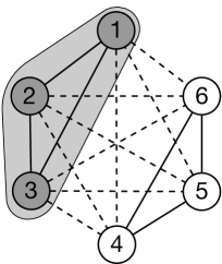
(b) $G^{\prime}$

Figure 1: Imbalanced Graph and Balanced Graph

For the signed networks, the most fundamental and dominant theory revealing the dynamics and construction of the signed networks is the structural balance theory [24, 25, 19, 20, 21, 14, 17, 22, 23]. The intuition underlying the structural balance theory can be described as the aphorisms: “The friend (resp. enemy) of my friend (resp. enemy) is my friend, the friend (resp. enemy) of my enemy (resp. friend) is my enemy”. Specifically, a signed network $G$ is structural balanced if $G$ can be split into two subgraphs such that the edges in the same subgraph are positive and the edges between subgraphs are negative [25]. In a signed network, an imbalanced sub-structure is unstable and tends to evolve into a balanced state. Consider the graph $G$ shown in Figure 1 (a). The negative edge between $v_{1}$ and $v_{2}$ makes $G$ imbalanced. $v_{1}$ and $v_{2}$ have a mutual “friend” $v_{3}$ and mutual “enemies” $v_{4}$, $v_{5}$ and $v_{6}$. It means $v_{1}$ and $v_{2}$ share more common grounds than differences. According to structural balance theory, $v_{1}$ and $v_{2}$ tend to be allies as time goes by. $G^{\prime}$ shown in Figure 1 (b) is the evolved balanced counterpart of $G$. In $G^{\prime}$, the sign of the edge between $v_{1}$ and $v_{2}$ becomes positive. $\{v_{1},v_{2},v_{3}\}$ and $\{v_{4},v_{5},v_{6}\}$ form two alliances and the edges in the same alliance are positive and the edges connecting different alliances are negative. As illustrated in this example, structural balance reflects the key characteristics of the signed networks.

According to the above analysis, clique model is a fundamental cohesive subgraph model in graph analysis, but there is no appropriate counterpart in the signed networks. Meanwhile, the structure of the signed networks is expected to be balanced based on the structure balance theory. Motivated by this, we propose a maximal balanced clique model in this paper. Formally, given a signed network $G$, a maximal balanced clique $C$ is a maximal subgraph of $G$ such that (1) $C$ is complete, i.e., every pair of vertices in $C$ has an edge. (2) $C$ is balanced, i.e., $C$ can be divided into two parts such that the edges in the same part are positive and the edges connecting two parts are negative. This definition not only catches the essence of the clique model in the unsigned networks but also guarantees that a detected clique is stable in the signed networks. In this paper, we aim to devise efficient algorithms to enumerate all maximal balanced cliques in a given signed network.

Moreover, in real signed networks, the number of maximal balanced cliques could be extremely large. For instance, in ”Douban” network which is a Chinese score service website, there are more than a million balanced cliques in it. However, in some applications, users prefer a unique and representative balanced clique with maximum size rather than all balanced cliques. Maximum clique search problem is a fundamental and hot research topic in graph analysis. In the literature, numerous studies have been conducted, such as maximum clique search [26, 27], maximum quasi-clique search [28], maximum bi-clique search[29], k*-partite clique with maximum edges[30], clique with maximum edge/vertex weight on weighted graph[31, 32]. Motivated by this, we aim to devise a maximum balanced clique search algorithm to find out the balanced clique with maximum vertex size, which can scale to large-scale real signed networks (with more than 100 million edges).

Applications. Balanced clique computation can be used in many applications, for example:

(1) Opinion leaders detection in opinion networks. Opinion leaders are people who are active in a community capturing the most representative opinions in the social networks [33]. In an opinion network, each vertex represents a user and there is a positive/negative edge between two vertices if one user support/dissent another user. A maximal balanced clique in an opinion network represents a group of users, such that these users actively involve in the opinion networks and have their clear standpoints. Hence, the users in the maximal balanced cliques are good candidates of opinion leaders in the opinion network.

(2) Finding international alliances-rivalries groups. The international relationships between nations can be modeled as a signed network, where each vertex represents a nation, positive and negative edges indicate alliances and rivalries, respectively. Computing the maximal balanced cliques in such networks reveals hostile groups of allied forces[14, 34]. We can extend it to find the alliances-rivalries commercial groups among business organizations similarly, such as {Pepsi, KFC} vs {Coke, McDonald}[35].

(3) Synonym and antonym groups discovery. In a word network, each vertex represents a word and there is a positive edge between two synonyms and a negative edge between two antonyms[36]. In such signed networks, our model can discover synonym groups that are antonymous with each other, such as, {interior, internal, intimate} and {away, foreign, outer, outside, remote}. These discovered groups may be further used in applications such as automatic question generation [37] and semantic expansion [38].

Contributions. In this paper, we make the following contributions:

(1) The first work to study the maximal balanced clique model. We formalize the balanced clique model in signed networks based on the structural balance theory. To the best of our knowledge, this is the first work considering the structural balance of the cliques in signed networks. We also prove the NP-Hardness of the problem.

(2) A new framework tailored for maximal balanced clique enumeration in signed networks. After investigating the drawbacks of the straightforward approach, we propose a new framework for the maximal balanced clique enumeration. Our new framework enumerates the maximal balanced cliques based on the signed network directly and its memory consumption is linear to the size of the input signed network.

(3) Two effective optimization strategies to further improve the enumeration performance. We explore two optimization strategies, in-enumeration optimization and pre-enumeration optimization, to further improve the enumeration performance. The in-enumeration optimization can avoid the exploration for unpromising vertices during the enumeration while the pre-enumeration techniques can prune unpromising vertices and edges before enumeration.

(4) An efficient maximum balanced clique search algorithm. To address the maximum balanced clique search problem, we first propose a baseline algorithm. In order to reduce the search space during the search process of baseline, we propose a search space partition-based algorithm $\mathsf{MBCSear}$-$\mathsf{SSP}$ by partitioning the whole search space into multiple search regions. In each search region, two size thresholds $\overline{\kappa}$ and $\underline{\kappa}$ are used to search the result matching the size requirement specific to this search region, such that the search space is limited into a small area. To further improve the efficiency of $\mathsf{MBCSear}$-$\mathsf{SSP}$ algorithm, we also explore three optimization strategies to prune invalid search branches and candidates during the search process.

(5) Extensive performance studies on real datasets. We first evaluate the performance of $\mathsf{MBCE}$ algorithms by conducting extensive experimental studies on real datasets. As shown in our experiments, the baseline approach only works on small datasets while our approach can complete the enumeration efficiently on both small and large datasets. Then, we evaluate the performance of our proposed $\mathsf{MBCS}$ algorithm. The baseline algorithm can not get the result within a reasonable time on large datasets, while our optimized algorithm shows high efficiency, effectiveness and scalability.

2 Related Work

Signed network analysis. Structural balance theory is originally introduced in [24] and generalized in the graph formation in [25, 19]. After that, structural balance theory is developed extensively [20, 21, 17, 22, 23]. In these works, it is interesting to mention that the authors in [22] model the evolving procedure of a signed network and theoretically prove that the network would evolve into a balanced clique when the mean value of the initial friendliness among the vertices $\mu\leq 0$. [39] provides a comprehensive survey on structural balanced theory.

Besides, a large body of literature on mining signed networks has been emerged. Among them, the most closely related work to ours is [40] in which an $(\alpha,k)$-clique model is proposed. Compared with our model, $(\alpha,k)$-clique model only considers the amount of positive and negative edges in the clique and the structural balance of the clique is totally ignored, which makes $(\alpha,k)$-clique model essentially different from our model. In [41], a $k$-balanced trusted clique model is proposed. Although the $k$-balanced trusted clique model has a similar name with our model, it ignores the negative edges in the clique, which means the information of the negative edges are totally missed.

Clique on unsigned networks. Clique model is one of the most fundamental cohesive subgraph models. [10] proposes an efficient algorithm for maximal clique enumeration based on backtracking search.[42] first considers the memory consumption during the maximal clique enumeration. Based on [10], more efficient algorithms are investigated [43, 11, 12].[11] proposes a novel branch pruning strategy, which can efficiently reduce the search space by ignoring the search process from the neighbors of the pivot. [44] reviews recently advances in maximal clique enumeration. Based on clique, other cohesive subgraph models are also studied, such as $k$-core [45], $k$-truss[46, 47], $k$-edge connected component[48, 49, 50], and $(r,s)$-nuclei [51, 52].

3 Problem Statement

In this paper, we consider an undirected and unweighted signed network $G=(V,E^{+},E^{-})$, where $V$ denotes the set of vertices, $E^{+}$ denotes the positive edges and $E^{-}$ denotes the negative edges connecting the vertices in $G$. We denote the number of vertices and number of edges by $n$ and $m$, respectively. For each vertex $v\in G$, let $N^{+}_{G}(v)$ represents the positive neighbors of $v$, and let $N^{-}_{G}(v)$ represents the negative neighbors of $v$. We use $d^{+}_{G}(v)$ and $d^{-}_{G}(v)$ to denote the positive and negative degree of $v$, respectively. We also use $N_{G}(v)$ and $d_{G}(v)$ to denote the neighbors and degree of $v$, i.e., $N_{G}(v)=N^{-}_{G}(v)\cup N^{+}_{G}(v)$ and $d_{G}(v)=d^{+}_{G}(v)+d^{-}_{G}(v)$. For simplicity, we omit G in the above notations if the context is self-evident.

Definition 3.1: (Balanced Network [25]) Given a signed network $G=(V,E^{+},E^{-})$, it’s balanced iff it can be split into two subgraphs $G_{L}$ and $G_{R}$, s.t. $\forall(u,v)\in E^{+}\rightarrow u,v\in G_{L}$ or $u,v\in G_{R}$, and $\forall(u,v)\in E^{-}\rightarrow u\in G_{L},v\in G_{R}$ or $u\in G_{R},v\in G_{L}$. $\Box$

Definition 3.2: (Maximal Balanced Clique) Given a signed network $G=(V,E^{+},E^{-})$, a maximal balanced clique $C$ is a maximal subgraph of $G$ that satisfies the following constraints:

• Complete: $C$ is complete, i.e, $\forall u,v\in C\rightarrow(u,v)\in E^{+}\cup E^{-}$.

• Balanced: $C$ is balanced, i.e, it can be split into two sub-cliques $C_{L}$ and $C_{R}$, s.t. $\forall u,v\in C_{L}$ or $u,v\in C_{R}\rightarrow(u,v)\in E^{+}$, and $\forall u\in C_{L},v\in C_{R}$ or $u\in C_{R},v\in C_{L}\rightarrow(u,v)\in E^{-}$.

$\Box$

Definition 3.3: (Maximum Balanced Clique) Given a signed network $G=(V,E^{+},E^{-})$, a maximum balanced clique $C^{*}$ in $G$ is a balanced clique with the maximum vertex size. $\Box$

Since many real applications require that the number of vertices in $C_{L}$ and $C_{R}$ is not less than a fixed threshold, we add a size constraint on $|C_{L}|$ and $|C_{R}|$ s.t. $|C_{L}|\geq k$ and $|C_{R}|\geq k$. With the size constraint, users can control the size of the returned maximal balanced cliques based on their specific requirements. We formalize the studied problems in the paper as follows:

Problem Statement. Given a signed network $G$ and an integer $k$,

• the maximal balanced clique enumeration ($\mathsf{MBCE}$) problem aims to compute all the maximal balanced cliques $C$ in $G$ s.t. $|C_{L}|\geq k$ and $|C_{R}|\geq k$ for $C$.

• the maximum balanced clique search ($\mathsf{MBCS}$) problem aims to compute the balanced clique $C^{*}$ in $G$ s.t. $|C^{*}_{L}|\geq k$, $|C^{*}_{R}|\geq k$ and $|C^{*}_{L}|+|C^{*}_{R}|$ is maximum.

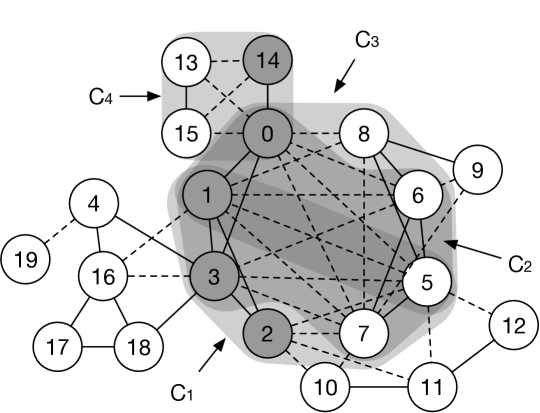
Figure 2: Maximal Balanced Clique in $G$ ($k=2$)

Example 3.1: Consider the signed network $G$ in Figure 2 in which positive/negative edges are denoted by solid/dashed lines. Assume $k$ = 2, there are 4 maximal balanced cliques in $G$, namely, $C_{1}=\{\{v_{1},v_{2},v_{3}\},\{v_{5},v_{7}\}\}$, $C_{2}=\{\{v_{0},v_{1},v_{3}\},\{v_{5},v_{6},v_{7}\}\}$, $C_{3}$ $=\{\{v_{0},v_{1}\},\{v_{5},v_{6},v_{8}\}\}$, $C_{4}=\{\{v_{0},v_{14}\},\{v_{13},v_{15}\}\}$, where vertices in $C_{L}$ and $C_{R}$ are marked with different colors. Among them, $C_{2}$ is the maximum balanced clique. $\Box$

Problem Hardness.The $\mathsf{MBCE}$ problem is NP-Hard, which can be proved following the NP-Hardness of maximal clique enumeration problem [53, 54]. Given an unsigned network $G=(V,E)$, we can transfer $G$ to a signed network $G^{\prime}$ as follows: we first keep all the vertices of $G$ in $G^{\prime}$ and all the edges of $G$ as positive edges in $G^{\prime}$; then, we add a new vertex $v$ to $G^{\prime}$ and connect $v$ to all vertices in $G^{\prime}$ with negative edges. It’s clear that each maximal clique $C$ in $G$ corresponds a maximal balanced clique $\{\{v\},C\}$ in $G^{\prime}$ (assume $k=1$), which means the maximal clique enumeration problem in $G$ can be reduced to the $\mathsf{MBCE}$ problem in $G^{\prime}$. As the maximal clique enumeration problem is NP-Hard [53, 54], our $\mathsf{MBCE}$ problem is also NP-Hard.

Similarly, reconsidering $G$ and $G^{\prime}$, the maximum clique $C^{*}$ in $G$ corresponds the maximum balanced clique $\{\{v\},C^{*}\}$ in $G^{\prime}$, and vice versa. As the maximum clique search problem is NP-Hard[27, 26], our $\mathsf{MBCS}$ problem is also NP-Hard.

4 A Baseline Algorithm for MBCE Problem

We first propose a baseline algorithm to address $\mathsf{MBCE}$ problem based on existing methods for maximal clique enumeration [12] and maximal biclique enumeration [55] in unsigned networks. For a signed network $G=(V,E^{+},E^{-})$, we can treat it as the combination of two unsigned networks $G^{+}=(V,E^{+})$ and $G^{-}=(V,E^{-})$. For any maximal balanced clique $C=\{C_{L},C_{R}\}$ in $G$, it is clear that $C_{L}$ (resp. $C_{R}$) is a clique in $G^{+}$ and the subgraph induced by vertices in $C_{L}$ and $C_{R}$ in $G^{-}$ is a biclique. Therefore, we can enumerate the maximal balanced cliques in $G$ in two steps: 1) compute all the maximal cliques in $G^{+}$ with [12]; 2) for each pair of the computed maximal cliques $C_{i}$ and $C_{j}$ in $G^{+}$, compute the maximal bicliques in the bipartite subgraph induced by the vertices in $C_{i}$ and $C_{j}$ in $G^{-}$ with [55]. The returned maximal bicliques in $G^{-}$ are the maximal balanced cliques in $G$.

Drawbacks of $\mathsf{baseline}$. Since $\mathsf{Baseline}$ does not consider the uniqueness of the signed networks and processes $\mathsf{MBCE}$ with the techniques for the unsigned networks, it has two drawbacks:

• Memory consumption. $\mathsf{Baseline}$ has to store all the maximal cliques in $G^{+}$ in memory. The number of maximal cliques could be exponential to the number of vertices [11], which makes $\mathsf{Baseline}$ unable to handle large networks.

• Efficiency. In $\mathsf{baseline}$, all the maximal cliques in $G^{+}$ are enumerated and every pair of maximal cliques are explored. The time complexity of $\mathsf{Baseline}$ is $O(T_{{\mathsf{Cli}}}+\eta^{2}\cdot T_{{\mathsf{BiCli}}})$, where $T_{{\mathsf{BiCli}}}$/$T_{{\mathsf{Cli}}}$ represent the time complexity of maximal (bi)clique enumeration, and $\eta$ is the number of enumerated maximal cliques in $G^{+}$. Considering the maximal (bi)clique enumeration is time-consuming and the number of maximal cliques could be very large, it is inefficient for $\mathsf{MBCE}$ problem.

5 A New Enumeration Framework

Revisiting $\mathsf{baseline}$, the root leading to its drawbacks discussed above is that it treats the signed network as a specific combination of two unsigned networks and utilizes the existing techniques designed for the unsigned networks. Therefore, we have to explore new techniques by considering the uniqueness of signed networks to overcome the drawbacks of $\mathsf{Baseline}$ and improve the efficiency of the enumeration. In this section, we present a new enumeration framework which aims to address the memory consumption problem. In next section, we further optimize the enumeration framework to improve the efficiency.

Lemma 5.1: Given a signed network $G$, for a balanced clique $C=\{C_{L},C_{R}\}$ in $G$, if there is a vertex $v$ in $G$ such that $\forall u\in C_{L}\rightarrow(v,u)\in E^{+}$ and $\forall w\in C_{R}\rightarrow(v,w)\in E^{-}$, then $C^{\prime}=\{C_{L}\cup\{v\},C_{R}\}$ is also a balanced clique in $G$.

According to Lemma 5, if we maintain a balanced clique $C=\{C_{L},C_{R}\}$, let $P_{L}$ be the set of vertices that are positive neighbors of all the vertices in $C_{L}$ and negative neighbors of all the vertices in $C_{R}$, let $P_{R}$ be the set of vertices that are positive neighbors of all the vertices in $C_{R}$ and negative neighbors of all the vertices in $C_{L}$, we can enlarge $C$ by adding vertices from $P_{L}$ and $P_{R}$ into $C_{L}$ and $C_{R}$, respectively. Furthermore, if we update the $P_{L}$ and $P_{R}$ based on the new $C_{L}$ and $C_{R}$ accordingly and repeat the above enlargement procedure, we can obtain a maximal balanced clique when no more vertices can be added into $C_{L}$ or $C_{R}$.

Algorithm 1 $\mathsf{MBCEnum}$ ($G=(V,E^{+},E^{-}),k$)

1:  ${\mathsf{Flag}}\leftarrow$ true;

2:  for each $v_{i}\in\{v_{0},v_{1},\cdots,v_{n-1}\}\in V$ do

3:     $C_{L}\leftarrow\{v_{i}\}$, $C_{R}\leftarrow\emptyset$

4:     $P_{L}\leftarrow N^{+}_{G}(v_{i})\cap\{v_{i+1},\cdots,v_{n-1}\}$;

5:     $P_{R}\leftarrow N^{-}_{G}(v_{i})\cap\{v_{i+1},\cdots,v_{n-1}\}$;

6:     $Q_{L}\leftarrow N^{+}_{G}(v_{i})\cap\{v_{0},\cdots,v_{i-1}\}$;

7:     $Q_{R}\leftarrow N^{-}_{G}(v_{i})\cap\{v_{0},\cdots,v_{i-1}\}$;

8:     $\mathsf{MBCEnumUtil}$ $(C_{L},C_{R},P_{L},P_{R},Q_{L},Q_{R})$;

9:  Procedure $\mathsf{MBCEnumUtil}$ ($C_{L},C_{R},P_{L},P_{R},Q_{L},Q_{R}$)

10:  if $P_{L}=\emptyset$ and $P_{R}=\emptyset$ and $Q_{L}=\emptyset$ and $Q_{R}=\emptyset$ then

11:     if $|C_{L}|\geq k$ and $|C_{R}|\geq k$ then

12:        output $C=\{C_{L},C_{R}\}$;

13:     return

14:  ${\mathsf{Flag}}\leftarrow!{\mathsf{Flag}}$;

15:  if ${\mathsf{Flag}}$ then

16:     for each $v\in$ $\mathsf{P_{L}}$ do

17:        ${\mathsf{MBCEnumUtil}}(C_{L}\cup\{v\},C_{R},N^{+}_{G}(v)\cap P_{L},N^{-}_{G}(v)\cap P_{R},N^{+}_{G}(v)\cap Q_{L},N^{-}_{G}(v)\cap Q_{R})$;

18:        $P_{L}\leftarrow P_{L}\setminus\{v\}$; $Q_{L}\leftarrow Q_{L}\cup\{v\}$;

19:     for each $v\in$ $\mathsf{P_{R}}$ do

20:        ${\mathsf{MBCEnumUtil}}(C_{L},C_{R}\cup\{v\},N^{-}_{G}(v)\cap P_{L},N^{+}_{G}(v)\cap P_{R},N^{-}_{G}(v)\cap Q_{L},N^{+}_{G}(v)\cap Q_{R})$;

21:        $P_{R}\leftarrow P_{R}\setminus\{v\}$; $Q_{R}\leftarrow Q_{R}\cup\{v\}$;

22:  else

23:     line 19-21; line 16-18;

Algorithm of $\mathsf{MBCEnum}$. Following the above idea, our algorithm for $\mathsf{MBCE}$ is shown in Algorithm 1. For each vertex $v_{i}$ in $G$ (line 2), we enumerate all the maximal balanced cliques containing $v_{i}$ (line 3-8). Note that $v_{0},v_{1},\dots,v_{n}$ are in the degeneracy order [56] of $G$. We use $C_{L}$ and $C_{R}$ to maintain the balanced clique, which are initialized with $v_{i}$ and $\emptyset$, respectively (line 3). Similarly, we also initialize $P_{L}$ and $P_{R}$ as discussed above (line 4-5). Moreover, we use $Q_{L}$ and $Q_{R}$ to record the vertices that have been processed to avoid outputting duplicate maximal balanced cliques (line 6-7). After initializing these six sets, we invoke procedure $\mathsf{MBCEnumUtil}$  to enumerate all the maximal balanced cliques containing $v_{i}$ (line 8).

Procedure $\mathsf{MBCEnumUtil}$ performs the maximal balanced clique enumeration based on the given six sets. If $P_{L}$, $P_{R}$, $Q_{L}$ and $Q_{R}$ are empty, which means current balanced clique $C=\{C_{L},C_{R}\}$ cannot be enlarged and it is a maximal balanced clique, $\mathsf{MBCEnumUtil}$ checks whether $C_{L}$ and $C_{R}$ satisfy the size constraint. If the size constraint is satisfied, it outputs the maximal balanced clique $C$ (line 11-12). Otherwise, $\mathsf{MBCEnumUtil}$ adds a vertex from $P_{L}$ to $C_{L}$, updates the corresponding $P_{L}$, $P_{R}$, $Q_{L}$ and $Q_{R}$, and recursively invokes itself to further enlarge the balanced clique (line 17). When $v\in P_{L}$ is processed, $v$ is removed from $P_{L}$ and added in $Q_{L}$ (line 18). Similar processing steps are applied on vertices in $P_{R}$ (line 19-21). Variable $\mathsf{Flag}$ (line 1) is used to control the order of adding new vertex into $C_{L}$ or $C_{R}$. With the switch operation in line 14, we can guarantee that we add vertex into $C_{L}$, then into $C_{R}$, recursively.

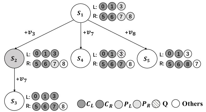
Figure 3: Search Tree for $\mathsf{MBCEnum}$

Example 5.1: The enumeration procedure of $\mathsf{MBCEnum}$ can be illustrated as a search tree. Figure 3 shows part of the search tree when we conduct the $\mathsf{MBCE}$ on $G$ in Figure 2 through $\mathsf{MBCEnum}$. $S_{1},S_{2},\dots$ represent different search states during the enumeration. At $S_{1}$, we assume that we have a balanced clique with $C_{L}$=$\{v_{0},v_{1}\}$, $C_{R}$=$\{v_{5},v_{6}\}\}$, $P_{L}$=$\{v_{3}\}$ and $P_{R}$=$\{v_{7},v_{8}\}$ at this state. We first grow search branch by adding $v_{3}$ into $C_{L}$. At $S_{2}$, $P_{L}$ is empty, $P_{R}=\{v_{7}\}$, hence, we add $v_{7}$ into $C_{R}$ at $S_{3}$ and obtain $C_{2}=\{\{v_{0},v_{1},v_{3}\},\{v_{5},v_{6},v_{7}\}\}$. Now, the search branch from $v_{3}$ is finished, we return to $S_{1}$ state. Since $v_{3}$ has been explored, it is removed to $Q_{L}$, $P_{L}$ is empty now. Then, we add $v_{7}$ from $P_{R}$ to $C_{R}$ at $S_{4}$. Due to $C_{2}$ has been found at $S_{3}$, current result at $S_{4}$ is not maximal and can not be output. Next, we return to $S_{1}$ and find $C_{3}=\{\{v_{0},v_{1}\},\{v_{5},v_{6},v_{8}\}\}$ by adding $v_{8}$ into $C_{R}$. Here, the search procedure at this search tree is finished. Other maximal balanced cliques can be found in a similar way. $\Box$

Based on Algorithm 1, it is clear that the memory consumption of our enumeration framework is linear to the size of the input signed network. Therefore, the drawback of large memory consumption in $\mathsf{Baseline}$ is avoided.

6 Enumeration Optimization Strategies

Although Algorithm 1 addresses the memory consumption problem in $\mathsf{MBCE}$, the efficiency of Algorithm 1 is disappointing. In this section, we present two optimization strategies, namely in-enumeration optimization and pre-enumeration optimization, to further improve the efficiency of the enumeration.

6.1 In-Enumeration Optimization

Branch Pruning. Branch pruning aims to prune the unfruitful branches in the search tree of Algorithm 1 to improve the performance.

Pivot Choosing. Consider the maximal balanced clique search procedure of Algorithm 1, assume that we currently have $C_{L}$, $C_{R}$, $P_{L}$ and $P_{R}$, and we add a vertex $v$ from $P_{L}$ to $C_{L}$ in line 17. After finishing the search starting from $v$, we do not need to further explore the positive neighbors of $v$ in the for loop of line 16 and the negative neighbors of $v$ in the for loop of line 19. The reasons are as follows: w.o.l.g, let $v^{\prime}$ be a positive neighbor of $v$, although we skip the maximal balanced clique search starting from $v^{\prime}$, these maximal balanced cliques containing $v^{\prime}$ must be explored by the searching branches starting $v$ or neighbors of $v^{\prime}$. Therefore skipping the search starting from $v$’s neighbors does not affect the correctness of Algorithm 1.

In this paper, to maximum the benefits of pivot technology, we define the local degree for a vertex $v\in P_{L}\cup Q_{L}(P_{R}\cup Q_{R})$ as $d_{l}(v)=|N^{+(-)}(v)\cap P_{L}|+|N^{-(+)}(v)\cap P_{R}|$, and we choose the vertex $v$ that satisfies $\max_{v\in V^{\prime}}\{d_{l}(v)\}$ as the pivot, where $V^{\prime}=P_{L}\cup P_{R}\cup Q_{L}\cup Q_{R}$.

Candidate Selection. In the search procedure of Algorithm 1, heuristically, search starting from a vertex with small local degree will have a short and narrow search branch, which means the search starting from the vertex will be finished very fast. Moreover, due to the search finish of the vertex, the vertex will be added into the excluded set and it can be used to further prune other search branches. Therefore, instead of adding vertices from $P_{L}$ and $P_{R}$ into $C_{L}$ and $C_{R}$ randomly in line 16 and 19 of Algorithm 1, we add vertices in the increasing order of their local degrees.

Early Termination. We consider different conditions that we can terminate the search early in Algorithm 1. For a balanced clique $C=\{C_{L},C_{R}\}$, the maximal possible size of $C_{L}$ ($C_{R}$) for the final maximal balanced clique is $|C_{L}|+|P_{L}|$ ($|C_{R}|+|P_{R}|$). Based on the size constraint of $k$, we have the following rule:

• ET Rule 1: If $|C_{L}|+|P_{L}|<k$ or $|C_{R}|+|P_{R}|<k$, we can terminate current search directly.

In Algorithm 1, we use $Q_{L}$ and $Q_{R}$ to store such vertices that the maximal balanced cliques containing them have been enumerated. Therefore, during the enumeration, if there exists a vertex $v\in Q_{L}(Q_{R})$ such that $P_{L}(P_{R})\subseteq N^{+}_{G}(v)$ and $P_{R}(P_{L})\subseteq N^{-}_{G}(v)$, then we can conclude that the maximal balanced cliques have been enumerated. Following this, we have our second rule:

• ET Rule 2: If $\exists v\in Q_{L}$, s.t., $P_{L}\subseteq N^{+}_{G}(v)$ and $P_{R}\subseteq N^{-}_{G}(v)$ or $\exists v\in Q_{R}$, s.t., $P_{R}\subseteq N^{+}_{G}(v)$ and $P_{L}\subseteq N^{-}_{G}(v)$, then we can terminate current search directly.

In a certain search of Algorithm 1, if all the vertices in $P_{L}$ ($P_{R}$) consist a clique formed by positive edges and every vertex in $P_{L}$ ($P_{R}$) has negative edges to all the vertices in $P_{R}$ ($P_{L}$), then $P_{L}$ and $P_{R}$ consist a balanced clique. Then, based on Definition 3, $C_{L}\cup P_{L}$ and $C_{R}\cup P_{R}$ consist a maximal balanced clique. Therefore, we have our third early termination rule:

• ET Rule 3: If $\forall p_{l}\in P_{L}$, s.t., $P_{L}\subseteq\{\{p_{l}\}\cup N^{+}_{G}(p_{l})\}$ and $P_{R}\subseteq N^{-}_{G}(p_{l})$ and $\forall p_{r}\in P_{R}$, s.t., $P_{R}\subseteq\{\{p_{r}\}\cup N^{+}_{G}(p_{r})\}$ and $P_{L}\subseteq N^{-}_{G}(p_{r})$, we can output $C=(C_{L}\cup P_{L},C_{R}\cup P_{R})$ and terminate current search directly.

Note that, in order to avoid outputting duplicate maximal balanced cliques, ET Rule 3 must be applied after ET Rule 2.

Algorithm of $\mathsf{MBCEnum^{*}}$. Utilizing the in-enumeration optimization strategies, we propose the optimized algorithm $\mathsf{MBCEnum^{*}}$. The pseudocode is omitted here due to space constraints.

Theorem 6.1: Given a signed network $G$, the time complexity of $\mathsf{MBCEnum^{*}}$ is $O(\sigma n\cdot 3^{\sigma/3})$, where $\sigma$ is the degeneracy number of $G$.

6.2 Pre-Enumeration Optimization

In pre-enumeration optimization, we aim to remove the unpromising vertices and edges that not contained in any maximal balanced clique. We explore two optimization strategies based on the neighbors of a vertex and the common neighbors of an edge.

Vertex Reduction. To reduce the size of a signed network, we first consider the neighbors of each vertex $v$, i.e., $N^{+}_{G}(v)$ and $N^{-}_{G}(v)$ to remove the unpromising vertices. We first define:

Definition 6.1: (($l,r$)-signed core) Given a signed network $G=(V,E^{+},E^{-})$, two integers $l$ and $r$, a ($l,r$)-signed core is a maximal subgraph $\mathcal{C}$ of $G$, s.t., $\min_{v\in\mathcal{C}}\{d^{+}_{\mathcal{C}}(v)\}=l$, $\min_{v\in\mathcal{C}}\{d^{-}_{\mathcal{C}}(v)\}=r$. $\Box$

Lemma 6.1: Given a signed network $G$ and threshold $k$, a maximal balanced clique satisfying the size constraint with $k$ is contained in a $(k-1,k)$-signed core.

Therefore, in order to compute the maximal balanced cliques in a given signed network $G$ with integer $k$, we only need to compute the maximal balanced cliques in the corresponding $(k-1,k)$-signed core of $G$. The remaining problem is how to efficiently compute the $(k-1,k)$-signed core. We propose a linear algorithm $\mathsf{VertexReduction}$ to address this problem.

Algorithm of $\mathsf{VertexReduction}$. Based on Definition 6.2, to compute the $(k-1,k)$-signed core in the signed network $G$, we only need to identify the vertices with $d^{+}_{G}(v)<k-1$ or $d^{-}_{G}(v)<k$ and remove them from $G$. Due to the removal of such vertices, more vertices will violate the degree constraints, we can further remove these vertices until no such kind of vertices exist in $G$.

Theorem 6.2: Given a signed network $G$ and an integer $k$, the time complexity of $\mathsf{VertexReduction}$ is $O(n+m)$.

Figure 4: Different types of common neighbors for $(u,v)$

Edge Reduction. In this part, we explore the opportunities to remove unpromising edges with respect to $\mathsf{MBCE}$ by considering the common neighbors of an edge formed by different types of edges. Specifically, for a positive/negative edge $(u,v)$, we define the edge common neighbor number:

Definition 6.2: (Edge Common Neighbor Number) Given a signed network $G=(V,E^{+},E^{-})$, for a positive edge $(u,v)$, we define:

• $\delta^{++}_{G}(u,v)=|\{w|(u,w)\in E^{+}\wedge(v,w)\in E^{+}\}|$

• $\delta^{--}_{G}(u,v)=|\{w|(u,w)\in E^{-}\wedge(v,w)\in E^{-}\}|$

for a negative edge $(u,v)$, we define:

• $\delta^{+-}_{G}(u,v)=|\{w|(u,w)\in E^{+}\wedge(v,w)\in E^{-}\}|$

• $\delta^{-+}_{G}(u,v)=|\{w|(u,w)\in E^{-}\wedge(v,w)\in E^{+}\}|$

$\Box$

Figure 4 shows the different types of common neighbors used in Definition 4. For a positive edge $(u,v)$, Figure 4 (a) and (b) show the common neighbor $w$ used in $\delta^{++}_{G}(u,v)$ and $\delta^{--}_{G}(u,v)$, respectively. For a negative edge $(u,v)$, Figure 4 (c) and (d) show the common neighbor $w$ used in $\delta^{+-}_{G}(u,v)$ and $\delta^{-+}_{G}(u,v)$, respectively. Note that $G$ is undirected and every edge is stored once in $G$. Based on Definition 4, we have the following lemma:

Lemma 6.2: Given a signed network $G$ and an integer $k$, let $G^{\prime}$ be the maximal sub-network of $G$ s.t.,

1. $\forall(u,v)\in E^{+}_{G^{\prime}}\rightarrow\delta^{++}_{G^{\prime}}(u,v)\geq k-2\wedge\delta^{--}_{G^{\prime}}(u,v)\geq k$;

2. $\forall(u,v)\in E^{-}_{G^{\prime}}\rightarrow\delta^{+-}_{G^{\prime}}(u,v)\geq k-1\wedge\delta^{-+}_{G^{\prime}}(u,v)\geq k-1$;

then, every maximal balanced clique $C=\{C_{L},C_{R}\}$ in $G$ satisfying the size constraint with $k$ is contained in $G^{\prime}$.

Algorithm of $\mathsf{EdgeReduction}$. With Lemma 4, in order to enumerate the maximal balanced cliques in a given signed network $G$ with respect $k$, we only need to keep the edges in $G^{\prime}$ shown in Lemma 4 and the positive/negative edges not in $G^{\prime}$ can be safely pruned. We first compute $\delta^{++}_{G}(u,v)$ and $\delta^{--}_{G}(u,v)$ for each positive edge of $G$ and $\delta^{+-}_{G}(u,v)$ and $\delta^{-+}_{G}(u,v)$ for each negative edge of $G$. Following Lemma 4, for each positive edge $(u,v)$ such that $\delta^{++}_{G}(u,v)<k-2$ or $\delta^{--}_{G}(u,v)<k$, we remove $(u,v)$. After that, we decrease the corresponding edge common neighbor numbers that have been changed due to the removal of $(u,v)$ for the edge incident to $(u,v)$ based on Definition 4. It’s similar to negative edges. The algorithm terminates when all the edges satisfy conditions in Lemma 4.

Theorem 6.3: Given a signed network $G$, an integer $k$, the time complexity of $\mathsf{EdgeReduction}$ is $O(m^{1.5})$.

7 Maximum Balanced Clique Search

Maximum clique search problem is a fundamental and hot research topic in graph analysis. In this section, we study the maximum balanced clique search problem.

7.1 A Baseline Approach

We first propose a baseline approach, namely $\mathsf{MBCSear}$, to compute the maximum balanced clique in the input graph. We continuously enumerate the maximal balanced cliques in the input graph and maintain the maximum balanced clique $C^{*}$ found so far. For each search branch ($C_{L},C_{R},P_{L},P_{R}$), if $|C_{L}|+|C_{R}|+|P_{L}|+|P_{R}|\leq\epsilon$, where $\epsilon=|C^{*}|$, we can terminate the branch. When the enumeration finishes, it is easy to verify that $C^{*}$ is the maximum balanced clique.

Drawbacks of $\mathsf{MBCSear}$. Although the straightforward approach can find the maximum balanced clique, the complexity of $\mathsf{MBCSear}$ is the same as that of $\mathsf{MBCEnum^{*}}$ in the worst case. The search space of $\mathsf{MBCSear}$ is huge. In details, the drawbacks of $\mathsf{MBCSear}$ are twofold.

• Lack of rigorous size constraints for $|C_{L}|$ and $|C_{R}|$. Given a signed graph $G$, during the search process, $\mathsf{MBCSear}$ only holds the size constraint $|C_{L}|+|C_{R}|+|P_{L}|+|P_{R}|>\epsilon$ for each search branch. However, when $\epsilon$ is small, most of search branches have $|C_{L}|+|C_{R}|+|P_{L}|+|P_{R}|$ larger than $\epsilon$ which causes the fail of size constraint for most search branches. Unfortunately, as our algorithm constantly searches larger result than at present, the value of $\epsilon$ is gradually increasing from a small value, which makes $\mathsf{MBCSear}$ has to search the result with large search space.

• Massive invalid search branches. Although the search branches meet the size constraint with $\epsilon$, the structure between $P_{L}$ and $P_{R}$ maybe sparse which will generates invalid search branches. Hence, during the search process, more pruning techniques is needed urgently. Moreover, the optimization strategies based on $k$ in $\mathsf{MBCEnum^{*}}$, like vertex reduction and edge reduction, are limited here, as $C^{*}$ usually has size much larger than $k$. Therefore, the remaining graph after reduction is still huge on large-scale signed network.

Main idea. In the further work, we aim to improve the efficiency of our algorithm.

• To address the first drawback of lacking of rigorous size constraints for $|C_{L}|$ and $|C_{R}|$, we can propose $\underline{\kappa}$ and $\overline{\kappa}$ as the lower bounds for $min\{|C_{L}|,|C_{R}|\}$ and $max\{|C_{L}|,|C_{R}|\}$, respectively. Then, we can get the balanced cliques with $|C_{L}|\geq\underline{\kappa}$ and $|C_{R}|\geq\overline{\kappa}$ within narrow search space (assume $|C_{L}|\leq|C_{R}|$). Under different value of $\underline{\kappa}$ and $\overline{\kappa}$, the search space is split into multiple partitions. Moreover, with initializing $\underline{\kappa}$ or $\overline{\kappa}$ as large value, we can search balanced cliques with large size as priority. Under large $\epsilon$ and rigorous bounds $\underline{\kappa}$ and $\overline{\kappa}$, the search space can be significantly reduced.

• To address the second drawback of massive invalid search branches, regarding to bounds $\epsilon$, $\underline{\kappa}$ and $\overline{\kappa}$, we can propose optimizations to forecast the size of balanced clique found in the current search branch to avoid invalid search branches and remove redundant vertices from candidates. Moreover, we can extend the vertex reduction and edge reduction of $\mathsf{MBCEnum^{*}}$ with new bounds to prune more useless vertices and edges.

7.2 Search Space Partition-based Framework

To improve the efficiency of our approach, regarding to the first drawback of $\mathsf{MBCSear}$, in this subsection, we propose a new maximum balance clique search framework $\mathsf{MBCSear}$-$\mathsf{SSP}$ with two lower bounds $\underline{\kappa}$ and $\overline{\kappa}$ for $|C_{L}|$ and $|C_{R}|$. Given certain value $\underline{\kappa}_{i}$ and $\overline{\kappa}_{i}$, a search region is denoted as $(\underline{\kappa}_{i},\overline{\kappa}_{i})$, the maximum balanced clique found in it should satisfies $|C_{L}|\geq\underline{\kappa}_{i}$ and $|C_{R}|\geq\overline{\kappa}_{i}$ if $|C_{L}|\leq|C_{R}|$ (otherwise, swap $L$ and $R$). Under different value of $\underline{\kappa}$ and $\overline{\kappa}$, the whole search space can be divided into several search regions. In each search region, we keep searching larger result than at present. When all search regions are explored, the final result $C^{*}$ can be found.

As our main idea, to search the result with large size as priority, for the first search region $(\underline{\kappa}_{0},\overline{\kappa}_{0})$, $\overline{\kappa}_{0}$ is initialized as a large integer value. Obviously, as $\overline{\kappa}_{0}$ value is large, benefited from the strict size constraint, most of search branches of $\mathsf{MBCSear}$ are ineligible now. Hence the result can be found quickly in this search region. Besides, to obey the size threshold $k$, we make $\underline{\kappa}_{0}=k$. Then, to cover the whole search space, for the later search regions, we keep increasing $\underline{\kappa}$ and decreasing $\overline{\kappa}$ until $\underline{\kappa}=\overline{\kappa}$. In another word, for $i<j$, $\underline{\kappa}_{i}\leq\underline{\kappa}_{j}$ and $\overline{\kappa}_{i}\geq\overline{\kappa}_{j}$.

Here, we first assign the possible maximum value to $\overline{\kappa}_{0}$, we have the following lemma:

Lemma 7.1: Given a signed network $G=(V,E^{+},E^{-})$, for every balanced clique, we have $max\{|C_{L}|,|C_{R}|\}\leq\sigma+1$, where $\sigma$ is the degeneracy number of $G^{+}$.

Proof.

In unsigned networks, the degeneracy number plus 1 is an upper bound for the maximum size of cliques[27]. Based on Definition 3, in a signed network $G=(V,E^{+},E^{-})$, for every balanced clique $C=\{C_{L},C_{R}\}$, $C_{L}$ and $C_{R}$ are traditional cliques in $G^{+}$. Therefore, $|C_{L}|$ and $|C_{R}|$ are must not greater than $\sigma+1$, respectively. ∎

Based on Lemma 7.2, we assign $(k,\sigma+1)$ to the first search region $(\underline{\kappa}_{0},\overline{\kappa}_{0})$. Then, in the later search region, we continue to seek larger balanced clique than the current one. However, not every search region can find a valid result. To skip invalid search regions, we have the following lemma:

Lemma 7.2: Given a signed network $G$, the maximum balanced clique found in the $i$-th search region $(\underline{\kappa}_{i},\overline{\kappa}_{i})$ is denoted by $C^{*}_{i}=\{C_{L}^{i},C_{R}^{i}\}$. Then, for the next search region $(\underline{\kappa}_{i+1},\overline{\kappa}_{i+1})$ , we have $\underline{\kappa}_{i+1}=|C^{*}_{i}|-\overline{\kappa}_{i}$.

Proof.

We prove it by contradiction. Following the $i$-th search region, in the next search region $(\underline{\kappa}_{i+1},\overline{\kappa}_{i+1})$, if we get a larger balanced clique $C^{*}_{i+1}=\{C_{L}^{i+1},C_{R}^{i+1}\}$ than $C^{*}_{i}$. Based on our search framework, we have $max\{|C_{L}^{i+1}|,|C_{R}^{i+1}|\}<\overline{\kappa}_{i}$, otherwise, $C^{*}_{i+1}$ will be found in the $i$-th search region rather than the $(i+1)$-th search region. Now, we assume $min\{|C_{L}^{i+1}|,|C_{R}^{i+1}|\}<|C^{*}_{i}|-\overline{\kappa}_{i}$. Combining with $max\{|C_{L}^{i+1}|,|C_{R}^{i+1}|\}<\overline{\kappa}_{i}$, we have $|C^{*}_{i+1}|=|C_{L}^{i+1}|+|C_{R}^{i+1}|<|C^{*}_{i}|$. Obviously, it is against with our premise that $C^{*}_{i+1}$ is larger than $C^{*}_{i}$. Therefore, the assumption for $min\{|C_{L}^{i+1}|,|C_{R}^{i+1}|\}<|C^{*}_{i}|-\overline{\kappa}_{i}$ does not hold. We get $min\{|C_{L}^{i+1}|,C_{R}^{i+1}\}\geq|C^{*}_{i}|-\overline{\kappa}_{i}$, i.e., $\underline{\kappa}_{i+1}=|C^{*}_{i}|-\overline{\kappa}_{i}$. ∎

Based on Lemma 7.2, after the $i$-th search region, the search regions with $\underline{\kappa}<|C^{*}_{i}|-\overline{\kappa}_{i}$ can be skipped directly.

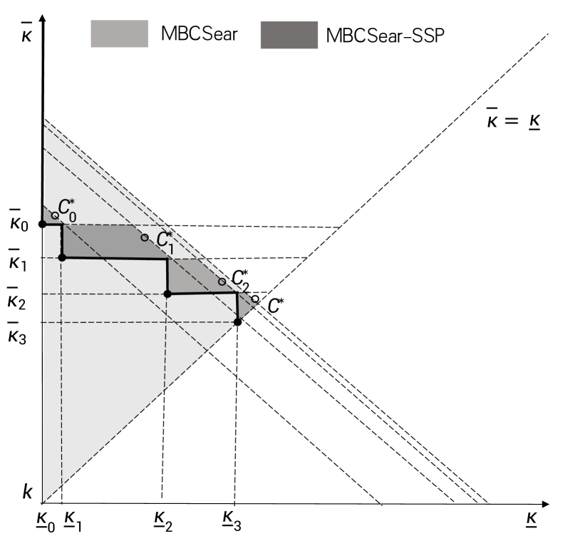
Figure 5: The search space of $\mathsf{MBCSear}$ and $\mathsf{MBCSear}$-$\mathsf{SSP}$

Algorithm 2 $\mathsf{MBCSear}$-$\mathsf{SSP}$ ($G=(V,E^{+},E^{-}),k$)

1:  compute degeneracy $\sigma$ of $G^{+}=(V,E^{+})$;

2:  $\epsilon\leftarrow 2k$; $\underline{\kappa}\leftarrow k$; $\overline{\kappa}\leftarrow\sigma+1$; $\overline{\kappa}^{\prime}\leftarrow-1$;

3:  while $\overline{\kappa}\geq\underline{\kappa}$ and $\overline{\kappa}<\overline{\kappa}^{\prime}$  do

4:     $\mathsf{MBCSear}$ $(G=(V,E^{+},E^{-}),\epsilon)$ with adding size constraints: $min\{\overline{L},\overline{R}\}<\underline{\kappa}$ or $max\{\overline{L},\overline{R}\}<\overline{\kappa}$;

5:     $\overline{\kappa}^{\prime}\leftarrow\overline{\kappa}$; $\underline{\kappa}\leftarrow max\{\epsilon-\overline{\kappa},k\}$; $\overline{\kappa}\leftarrow max\{Dec(\overline{\kappa}),\underline{\kappa}\}$;

Algorithm of $\mathsf{MBCSear}$-$\mathsf{SSP}$. Following the above idea, the new maximum balanced clique search algorithm $\mathsf{MBCSear}$-$\mathsf{SSP}$ is shown at Algorithm 2. Given a signed network $G=(V,E^{+},E^{-})$ and size threshold $k$, we first compute the degeneracy number $\sigma$ of $G^{+}=(V,E^{+})$ (line 1). We initialize $\epsilon=2k$, $\underline{\kappa}=k$, $\overline{\kappa}=\sigma+1$ (line 2). Then, in each search region, Algorithm 2 invokes $\mathsf{MBCSear}$ to find the maximum balanced clique in current search region with adding size constraints: $min\{\overline{L},\overline{R}\}<\underline{\kappa}$ or $max\{\overline{L},\overline{R}\}<\overline{\kappa}$ on each search branch. For the next search region, we let $\underline{\kappa}=max\{\epsilon-\overline{\kappa},k\}$ (line 5), since the size threshold $k$ is held for $C_{L}$ and $C_{R}$ as well. For the next value of $\overline{\kappa}$, $\overline{\kappa}=max\{Dec(\overline{\kappa}),\underline{\kappa}\}$ , where $Dec(\overline{\kappa})$ is used to decrease $\overline{\kappa}$. When $\overline{\kappa}<\underline{\kappa}$, let $\overline{\kappa}$=$\underline{\kappa}$. The search process finishes when $\overline{\kappa}=\underline{\kappa}$ and $\overline{\kappa}$ can not be reduced anymore, since if $\overline{\kappa}$ is unchanged, this search region is covered by the previous region already(line 3). When the search process of the final search region is finished, Algorithm 2 terminates and returns the maximum balanced clique $C^{*}$ in $G$.

Then, we discuss how $Dec(\overline{\kappa})$ decreases the value of $\overline{\kappa}$. The total running time of $\mathsf{MBCSear}$-$\mathsf{SSP}$ can be formulated as $T=\Sigma^{\omega}_{i=0}{t_{i}}$, where $\omega$ is the number of search regions and $t_{i}$ is the partial running time of the $i$-th search region. In this paper, to keep the efficiency of $\mathsf{MBCSear}$-$\mathsf{SSP}$, we give a heuristic way to decrease $\overline{\kappa}$. In detail, if the last search region is time-consuming (set time threshold like 20 seconds), to make the total running time $T$ as small as possible, we reduce the amount of search regions $\omega$ by decreasing $\overline{\kappa}$ by a large value, i.e., $Dec(\overline{\kappa})=\lceil\frac{\overline{\kappa}}{2}\rceil$, otherwise, $Dec(\overline{\kappa})=\overline{\kappa}-2$.

Now, we compare the search space between $\mathsf{MBCSear}$ and $\mathsf{MBCSear}$-$\mathsf{SSP}$. As shown at Figure 5, since $C^{*}$ is the maximum balanced clique, $\mathsf{MBCSear}$ searches all balanced cliques with size less than $C^{*}$ until $C^{*}$ is found. The search space of $\mathsf{MBCSear}$ is shown at Figure 5. For the search space of $\mathsf{MBCSear}$-$\mathsf{SSP}$, benefited from the tight bounds for $|C_{L}|$ and $|C_{R}|$ at each search region, $\mathsf{MBCSear}$-$\mathsf{SSP}$ searches local maximum balanced clique within small search space. For instance, as shown at Figure 5, it finds the current maximum balanced clique $C^{*}_{0}$ in the first search region. Then, in the second search region, it searches balanced cliques with $\overline{\kappa}_{1}\leq|C_{R}|<\overline{\kappa}_{0}$ and $|C_{L}|\geq\overline{\kappa}_{1}$ (assume $|C_{L}|\leq|C_{R}|$) until $C^{*}_{1}$ is found. As shown at Figure 5, the search space of $\mathsf{MBCSear}$-$\mathsf{SSP}$ is much smaller than $\mathsf{MBCSear}$.

Example 7.1: Reconsidering the signed network $G$ in Figure 2, $k=2$, Algorithm 2 first computes degeneracy number $\sigma$ of $G^{+}$, get $\sigma=2$. So, the first search region is $(2,3)$. Algorithm 2 find result $C^{*}_{0}=\{\{v_{0},v_{1},v_{3}\},\{v_{5},v_{6},v_{7}\}\}$ at first, $\epsilon=6$. Then, based on Lemma 7.2, $\underline{\kappa}_{1}$ is 3. As we should keep $\overline{\kappa}\geq\underline{\kappa}$, $\overline{\kappa}_{1}$ is 3 as well. However, as the value of $\overline{\kappa}$ is unchanged, this search region is covered by the first search region. Hence, Algorithm 2 is terminated and returns $C^{*}_{0}$ as $C^{*}$. Comparing with $\mathsf{MBCSear}$, the search space of $\mathsf{MBCSear}$-$\mathsf{SSP}$ is reduced from $(2,2)$ to $(2,3)$. $\Box$

7.3 Optimization Strategies

Regarding to the second drawback of $\mathsf{MBCSear}$ on massive invalid search branches in each search region, in this subsection, we explore the chance to further improve the efficiency of our approach. Under our rigorous lower bounds $\underline{\kappa}$ and $\overline{\kappa}$, we first propose two optimization strategies, coloring-based branch pruning and vertex domination-based candidate pruning, to prune invalid search branches and remove meaningless vertices from candidates. Then, we extend the vertex$\&$edge reduction technologies of $\mathsf{MBCE}$ to prune more unnecessary vertices and edges in advance.

7.3.1 Coloring-based Branch Pruning

Given a search region $(\underline{\kappa},\overline{\kappa})$ and a search branch, if the upper bound of the balanced clique size in current search branch is less than the lower bounds $\underline{\kappa}$, $\overline{\kappa}$ and $\epsilon$, current search branch can be pruned directly. Looking back to $\mathsf{MBCSear}$, it uses the candidates size to form the upper bound. However, this upper bound is too loose, because although the number of candidates is large, the connectivity between candidates maybe sparse, which will lead to many invalid search branches. Hence, now, we aim to propose a tighter upper bound based on vertex coloring.

Definition 7.1: (Vertex Coloring[57]) Given a graph $G$, vertex coloring in $G$ aims to assign colors to each vertex such that vertices are different in color from their neighbors. The amount of colors needed in $G$ is named chromatic number, denoted by $\gamma(G)$. $\Box$

Lemma 7.3: Given a search branch ($C_{L},C_{R},P_{L},P_{R}$), the maximum balanced clique from this branch is denoted as $C^{\prime}=\{C^{\prime}_{L},C^{\prime}_{R}\}$, we have that $|C^{\prime}_{L}|\leq\gamma(\mathbb{G}_{L})+|C_{L}|$, $|C^{\prime}_{R}|\leq\gamma(\mathbb{G}_{R})+|C_{R}|$, where $\mathbb{G}_{L(R)}$ is the positive subgraph produced by $P_{L(R)}$.

Proof.

Given a graph $G$, the chromatic number $\gamma(G)$ is an upper bound of the maximum size of cliques in $G$[27]. Based on it, the lemma can be proved. ∎

Based on Lemma 7.3.1, if the upper bound does not meet the size requirements of current search region, i.e., $min\{\gamma(\mathbb{G}_{L})+|C_{L}|,\gamma(\mathbb{G}_{R})+|C_{R}|\}<\underline{\kappa}$ or $max\{\gamma(\mathbb{G}_{L})+|C_{L}|,\gamma(\mathbb{G}_{R})+|C_{R}|\}<\overline{\kappa}$ or $\gamma(\mathbb{G}_{L})+|C_{L}|+\gamma(\mathbb{G}_{R})+|C_{R}|\leq\epsilon$, the search branch can be early terminated directly.

Algorithm of $\mathsf{ColoringPrune}$. We propose $\mathsf{ColoringPrune}$ algorithm to prune search branches. The pseudocode is shown at Algorithm 3. It first computes $\gamma(\mathbb{G}_{L})$ and $\gamma(\mathbb{G}_{R})$ (line 1-8). Then it returns $\mathsf{true}$ if the upper bound does not meet the size requirements, which means this search branch can be pruned directly, otherwise, returns $\mathsf{false}$ (line 9-11).

Algorithm 3 ${\mathsf{ColoringPrune}}(C_{L},C_{R},P_{L},P_{R},\epsilon,\underline{\kappa},\overline{\kappa}$)

1:  $\mathbb{G}_{L}\leftarrow G^{+}(P_{L})$; $\mathbb{G}_{R}\leftarrow G^{+}(P_{R})$;

2:  $\gamma(\mathbb{G}_{L(R)})$ $\leftarrow 0$; $col(v)\leftarrow 0$ for each $v\in P_{L(R)}$;

3:  for each $v\in P_{L(R)}$ do

4:     $col(v)\leftarrow 1$;

5:     while $\exists u\in N_{\mathbb{G}_{L(R)}}(v)$, s.t., $col(u)=col(v)$ do

6:        $col(v)\leftarrow col(v)+1$;

7:     if $col(v)>\gamma(\mathbb{G}_{L})$ then

8:        $\gamma(\mathbb{G}_{L(R)})\leftarrow\gamma(\mathbb{G}_{L(R)})+1$;

9:  if $min\{\gamma(\mathbb{G}_{L})+|C_{L}|,\gamma(\mathbb{G}_{R})+|C_{R}|\}<\underline{\kappa}$ or $max\{\gamma(\mathbb{G}_{L})+|C_{L}|,\gamma(\mathbb{G}_{R})+|C_{R}|\}<\overline{\kappa}$ or $\gamma(\mathbb{G}_{L})+|C_{L}|+\gamma(\mathbb{G}_{R})+|C_{R}|\leq\epsilon$  then

10:     return true;

11:  return false;

Theorem 7.1: The space complexity of Algorithm 3 is $O(|P_{L}|+|P_{R}|+|E_{\mathbb{G}_{L}}|+|E_{\mathbb{G}_{R}}|)$, the time complexity is $O(|P_{L}|+|P_{R}|+|E_{\mathbb{G}_{L}}|+|E_{\mathbb{G}_{R}}|)$.

Note that Algorithm 3 can be directly applied to ${\mathsf{MBCE}}$ problem with $\underline{\kappa}=k$, $\overline{\kappa}=k$, $\epsilon=2k$. However, since $k$ is usually small, the effectiveness of Algorithm 3 is limited in ${\mathsf{MBCE}}$ problem.

7.3.2 Vertex Domination-based Candidate Pruning

To further improve the efficiency, we reduce the number of candidates in $P_{L}$ and $P_{R}$ at each search branch by pruning invalid vertices from candidates. Our key thought is that if we have the prior knowledge to know that vertex $v$ forms balanced clique with size larger than that of vertex $u$, then, $u$ is dominated by $v$, denoted by $u\in\Phi_{v}$, the search relevant to $u$ can be skipped. Simplely, for each search branch, we can use the local neighborhood between candidates to figure out the domination relationship, i.e., if $N_{l}(u)\subseteq N_{l}(v)$, then $u\in\Phi_{v}$. Then, we have:

Lemma 7.4: Given a signed network $G$ and a search branch with candidate sets $P_{L}$ and $P_{R}$, for each vertex $v\in P_{L}\cup P_{R}$, if $v$ is dominated, the sub-search branch from $v$ can be skipped.

Proof.

Given a search branch, for vertices $u,v$ in candidates such that $u\in\Phi_{v}$, we use $C_{v}$ and $C_{u}$ to indicate the balanced cliques maintaining $v$ and $u$, respectively. Due to $N_{l}(u)\subseteq N_{l}(v)$, then $C_{u}\setminus\{u\}\subseteq C_{v}\setminus\{v\}$, i.e., $|C_{u}|\leq|C_{v}|$. Hence $u$ won’t belong to any balanced clique larger than $C_{v}$. The search from $u$ can be skipped. ∎

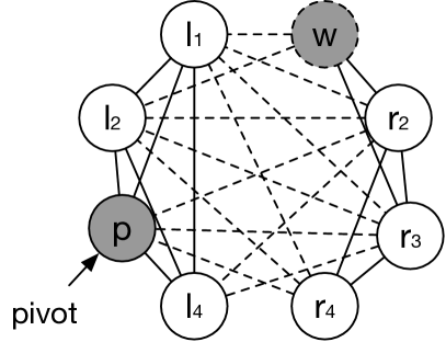
(a) Case 1$\&$3

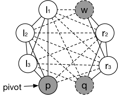
(b) Case 2$\&$4

Figure 6: Vertex Domination Cases

The vertex domination can be computed with adjacency list join operation. The time complexity of computing vertex domination at single search branch is $O(\mathrm{C_{\mathbb{n}}^{2}}\cdot(\mathbb{n}-1))=O(\mathbb{n}^{3})$, where $\mathbb{n}=|P_{L}|+|P_{R}|$, which is time-consuming. Moreover, the amount of search branches is huge. To obtain the vertex domination effectively, in this paper, we only consider four special cases based on pivot technique, which can be computed within const time. The four special cases are introduced as follows, $p$ is the selected pivot.

• Case 1: If $p\in Q_{L}\cup Q_{R}$ and $newP_{L}\cup newP_{R}=\{w\}$, then $\Phi_{p}=\{w\}$.

• Case 2: If $p\in Q_{L}\cup Q_{R}$, $newP_{L}\cup newP_{R}=\{w,q\}$ and $(w,q)\notin E$, then, $\Phi_{p}=\{w,q\}$.

• Case 3: If $p\in P_{L}\cup P_{R}$, $newP_{L}\cup newP_{R}=\{p,w\}$, then, $\Phi_{p}=\{w\}$.

• Case 4: If $p\in P_{L}\cup P_{R}$, $newP_{L}\cup newP_{R}=\{p,w,q\}$ and $(w,q)\notin E$, then, $\Phi_{p}=\{w,q\}$.

Figure 6 shows the four special cases of vertex domination, respectively. For case 1$\&$3(Figure 6(a)), $p$ is selected as pivot, then, the surviving candidate is $w$ as other vertices are $p$’s neighbors. Since $N_{l}(w)\subseteq N_{l}(p)$, $w$ is dominated by $p$. For case 2$\&$4(Figure 6(b)), $w$ and $q$ are two surviving candidates with pivot $p$, as $(w,q)\notin E$, they will not appear at a common balanced clique, hence, $N_{l}(w)\subseteq N_{l}(p)$, $N_{l}(q)\subseteq N_{l}(p)$, $\Phi_{p}=\{w,q\}$.

Based on Lemma 7.3.2, when we meet the above four special cases of vertex domination, we skip the searches from vertices in $\Phi_{p}$ by deleting them from candidate sets, this process only consumes const time. In this way, the invalid candidates can be further pruned effectively.

7.3.3 Vertex$\&$Edge Reduction Variants

Although the optimization strategies proposed in $\mathsf{MBCE}$ algorithm, like vertex reduction and edge reduction, are still applicable for $\mathsf{MBCSear}$, they only ensure that $C_{L}$ and $C_{R}$ are not less than $k$ but lack of binding force of our new size bounds $\underline{\kappa}$, $\overline{\kappa}$ and $\epsilon$. Moreover, the value of $\overline{\kappa}$, $\underline{\kappa}$ and $\epsilon$ are much larger than $k$, especially for $\overline{\kappa}$ and $\epsilon$, which makes the effectiveness of the reduction optimizations is limited in $\mathsf{MBCS}$ problem. Hence, we extend the vertex reduction and edge reduction such that they can support tighter bounds to prune more vertices and edges.

Vertex reduction variant. We first propose the vertex reduction variant with considering the degree of vertices. We have the following lemma:

Lemma 7.5: Given a signed network $G=(V,E^{+},E^{-})$, a search region $(\underline{\kappa}_{i},\overline{\kappa}_{i})$ and $\epsilon$, $\mathbb{G}=(\mathbb{V},\mathbb{E^{+}},\mathbb{E^{-}})$ is a subgraph of $G$, s.t., $(a)\forall v\in\mathbb{V},min\{d^{+}_{\mathbb{G}}(v)+1,d^{-}_{\mathbb{G}}(v)\}\geq\underline{\kappa}_{i},max\{d^{+}_{\mathbb{G}}(v)+1,d^{-}_{\mathbb{G}}(v)\}\geq\overline{\kappa}_{i}$; $(b)\forall v\in\mathbb{V},d^{+}_{\mathbb{G}}(v)+d^{-}_{\mathbb{G}}(v)+1>\epsilon$. We have $C^{*}_{i}\subseteq\mathbb{G}$.

Proof.

Given a search region $(\underline{\kappa}_{i},\overline{\kappa}_{i})$, let $C^{*}_{i}=\{C_{L},C_{R}\}$ is the maximum balanced clique in current search region. Based on Algorithm 2, $C^{*}_{i}=\{C_{L},C_{R}\}$ should satisfy $min\{|C_{L}|,|C_{R}|\}\geq\underline{\kappa}_{i}$ and $max\{|C_{L}|,|C_{R}|\}\geq\overline{\kappa}_{i}$. Meanwhile, based on Definition 3, $\forall v\in C_{L}$, $d_{C^{*}_{i}}^{+}(v)=|C_{L}|-1$, $d_{C^{*}_{i}}^{-}(v)=|C_{R}|$. $\forall v\in C_{R}$, $d_{C^{*}_{i}}^{+}(v)=|C_{R}|-1$, $d_{C^{*}_{i}}^{-}(v)=|C_{L}|$. Combining them, we get $min\{d^{+}_{C^{*}_{i}}(v)+1$, $d^{-}_{C^{*}_{i}}(v)\}\geq\underline{\kappa}$, $max\{d^{+}_{C^{*}_{i}}(v)+1$, $d^{-}_{C^{*}_{i}}(v)\}\geq\overline{\kappa}$. Moreover, as $C^{*}_{i}$ is the current maximum balanced clique, the degree of vertices in $C^{*}_{i}$ should not less than $\epsilon$. ∎

Algorithm of $\mathsf{VertexReduction^{+}}$. Based on Lemma 7.3.3, we can reduce the size of the candidate sets by continuously deleting the vertices that do not meet the degree constraints in Lemma 7.3.3. We propose $\mathsf{VertexReduction^{+}}$ algorithm, the pseudocode is shown at Algorithm 4. It continuously removes vertices until all vertices left in candidate sets meet the degree constraints.

Algorithm 4 ${\mathsf{VertexReduction^{+}}}(C_{L},C_{R},P_{L},P_{R},\epsilon,\underline{\kappa},\overline{\kappa}$)

1:  $V^{\prime}\leftarrow P_{L}\cup P_{R}$; $\mathbb{G}\leftarrow G(V^{\prime})$ ;

2:  while $\exists v\in P_{L(R)}$, s.t. $min\{d^{+}_{\mathbb{G}}(v)+1+|C_{L(R)}|,d^{-}_{\mathbb{G}}(v)+|C_{R(L)}|\}<\underline{\kappa}$ or $max\{d^{+}_{\mathbb{G}}(v)+1+|C_{L(R)}|,d^{-}_{\mathbb{G}}(v)+|C_{R(L)}|\}<\overline{\kappa}$ or $d^{+}_{\mathbb{G}}(v)+1+d^{-}_{\mathbb{G}}(v)+|C_{L}|+|C_{R}|\leq\epsilon$  do

3:     for each $u\in N^{+}_{\mathbb{G}}(v)$ do

4:        $d^{+}_{\mathbb{G}}(u)\leftarrow d^{+}_{\mathbb{G}}(u)-1$;

5:     for each $u\in N^{-}_{\mathbb{G}}(v)$ do

6:        $d^{-}_{\mathbb{G}}(u)\leftarrow d^{-}_{\mathbb{G}}(u)-1$;

7:     $\mathbb{G}\leftarrow\mathbb{G}\setminus v$;

8:     $P_{L(R)}\leftarrow P_{L(R)}\setminus v$;

Theorem 7.2: The space complexity of Algorithm 4 is $O(|P_{L}|+|P_{R}|+|E^{+}_{\mathbb{G}}|+|E^{-}_{\mathbb{G}}|)$. The time complexity of Algorithm 4 is $O(|P_{L}|+|P_{R}|+|E^{+}_{\mathbb{G}}|+|E^{-}_{\mathbb{G}}|)$, where $\mathbb{G}=G(P_{L}\cup P_{R})$.

Edge reduction variant. After the vertex reduction variant, we extend the edge reduction now. Inspired by the edge reduction technology utilized in $\mathsf{MBCE}$, we continue to explore the edge reduction under a certain search region. Reconsidering the edge common neighbor number introduced at Definition 4, we have the following lemma:

Lemma 7.6: Given a signed network $G$, a search region $(\underline{\kappa}_{i},\overline{\kappa}_{i})$ and $\epsilon$, $\mathbb{G}=(\mathbb{V},\mathbb{E^{+}},\mathbb{E^{-}})$ is a subgraph of $G$, s.t.,

• $\forall(u,v)\in\mathbb{E^{+}}\rightarrow min\{\delta^{++}_{\mathbb{G}}(u,v)+2,\delta^{--}_{\mathbb{G}}(u,v)\}\geq\underline{\kappa}_{i}\wedge max\{\delta^{++}_{\mathbb{G}}(u,v)+2,\delta^{--}_{\mathbb{G}}(u,v)\}\geq\overline{\kappa}_{i}$;

• $\forall(u,v)\in\mathbb{E^{-}}\rightarrow min\{\delta^{+-}_{\mathbb{G}}(u,v)+1,\delta^{-+}_{\mathbb{G}}(u,v)+1\}\geq\underline{\kappa}_{i}\wedge max\{\delta^{+-}_{\mathbb{G}}(u,v)+1,\delta^{-+}_{\mathbb{G}}(u,v)+1\}\geq\overline{\kappa}_{i}$.

Then, we have $C^{*}_{i}\subseteq\mathbb{G}$

Algorithm of $\mathsf{EdgeReduction^{+}}$. Based on Lemma 4, we propose $\mathsf{EdgeReduction^{+}}$ algorithm. Given a signed network $G=(V,E^{+},E^{-})$, a search region $(\underline{\kappa}_{i},\overline{\kappa}_{i})$ and $\epsilon$, before the search starts, it removes the invalid edges that do not meet the requirements for the edge common neighbor number in Lemma 4 until no more edges can be pruned. The pseudocode is omitted here. The time complexity of $\mathsf{EdgeReduction^{+}}$ is $O(m^{1.5})$.

7.3.4 The Optimized Algorithm

Utilizing the above optimization strategies, i.e., coloring-based branch pruning, vertex domination-based candidate pruning and vertex&edge reduction variants, we propose our optimized algorithm $\mathsf{MBCSear^{*}}$ to search maximum balanced clique in a given search region. The pseudocode is shown at Algorithm 5. Given a search region $(\underline{\kappa}$,$\overline{\kappa})$, for each search branch in this region, it first prunes candidates in $P_{L}$ and $P_{R}$ by invoking $\mathsf{VertexReduction^{+}}$ algorithm (line 4). Then, the surviving candidate sets are judged to see whether it meets the size requirements (line 5-7). If the candidate sets and explored sets are both empty, we get a larger result and return it (line 8-11). Otherwise, Algorithm 5 tries to prune invalid branch by invoking $\mathsf{ColoringPrune}$ (line 12-13). After that, it chooses the pivot and distinguishes the four special cases for vertex domination to further prune candidates (line 18-27). Then, it continuously search larger balanced clique in the remaining candidates by recursively calling itself. When all search branches are finished, Algorithm 5 can get the maximum balanced clique in the given search region.

Algorithm 5 $\mathsf{MBCSear^{*}}$ ($G=(V,E^{+},E^{-}),\epsilon$)

1:  for each $v\in V$ do

2:     initialize $C_{L},C_{R},P_{L},P_{R},Q_{L},Q_{R}$;

3:     $\mathsf{MBCSearUtil^{*}}$ $(C_{L},C_{R},P_{L},P_{R},Q_{L},Q_{R},\epsilon)$; Procedure $\mathsf{MBCSearUtil^{*}}$ ($C_{L}$, $C_{R}$, $P_{L}$, $P_{R}$, $Q_{L}$, $Q_{R}$, $\epsilon$) // Vertex Reduction Varint   

4:  ${\mathsf{VertexReduction^{+}}}(C_{L},C_{R},P_{L},P_{R},\epsilon,\underline{\kappa},\overline{\kappa})$;

5:  $\overline{L}\leftarrow|C_{L}|+|P_{L}|$; $\overline{R}\leftarrow|C_{R}|+|P_{R}|$;

6:  if $\overline{L}+\overline{R}\leq\epsilon$ or $min\{\overline{L},\overline{R}\}<\underline{\kappa}$ or $max\{\overline{L},\overline{R}\}<\overline{\kappa}$ then

7:     return;

8:  if $P_{L}=\emptyset$ and $P_{R}=\emptyset$ and $Q_{L}=\emptyset$ and $Q_{R}=\emptyset$ then

9:     $C^{*}\leftarrow\{C_{L},C_{R}\}$;

10:     $\epsilon\leftarrow|C_{L}|+|C_{R}|$;

11:     return; // Coloring-based Branch Pruning   

12:  if ${\mathsf{ColoringPrune}}(C_{L},C_{R},P_{L},P_{R},\epsilon,\underline{\kappa},\overline{\kappa})$ then

13:     return;

14:  $p\leftarrow{\mathsf{argmax}}_{v\in P_{L}\cup P_{R}\cup Q_{L}\cup Q_{R}}\{d_{l}(v)\}$;

15:  // assume $p$ from $P_{L}\cup Q_{L}$ ($P_{R}\cup Q_{R}$ )

16:  $newP_{L}\leftarrow P_{L}\setminus N^{+(-)}_{G}(p)$;

17:  $newP_{R}\leftarrow P_{R}\setminus N^{-(+)}_{G}(p)$; // Vertex Domination-based Candidate Pruning    // Case 1   

18:  if $p\in Q_{L(R)}$ and $|newP_{L}|+|newP_{R}|=1$ then

19:     return; // Case 2   

20:  if $p\in Q_{L(R)}$ and $|newP_{L}|+|newP_{R}|=2$ then

21:     if $w,q\in newP_{L}\cup newP_{R}$ and $(w,q)\notin E$ then

22:        return; // Case 3   

23:  if $p\in P_{L(R)}$ and $|newP_{L}|+|newP_{R}|=2$ then

24:     $newP_{L(R)}\leftarrow\{p\}$; $newP_{R(L)}\leftarrow\emptyset$; // Case 4   

25:  if $p\in P_{L(R)}$ and $|newP_{L}|+|newP_{R}|=3$ then

26:     if $w,q\in newP_{L}\cup newP_{R}$ and $(w,q)\notin E$ then

27:        $newP_{L(R)}\leftarrow\{p\}$; $newP_{R(L)}\leftarrow\emptyset$;

28:  search result within $newP_{L}$ and $newP_{R}$ as $\mathsf{MBCEnum}$;

Based on $\mathsf{MBCSear^{*}}$ algorithm, we are ready to propose the formal optimized algorithm $\mathsf{MBCSear}$-$\mathsf{SSP^{*}}$, the pseudocode is shown at Algorithm 6. Given a signed network $G=(V,E^{+},E^{-})$ and size threshold $k$, for each search region $(\overline{\kappa},\underline{\kappa})$, the algorithm first invokes $\mathsf{EdgeReduction^{+}}$ to reduce the graph size by removing invalid edges before search start (line 4). Then, it invokes Algorithm 5 to search the maximum balanced clique in current search region (line 5). In the end, when finish the search in all search regions, it gets the maximum balanced clique $C^{*}$ in $G$ and terminates.

Algorithm 6 $\mathsf{MBCSear}$-$\mathsf{SSP^{*}}$ ($G=(V,E^{+},E^{-}),k$)

1:  compute degeneracy $\sigma$ of $G^{+}=(V,E^{+})$;

2:  $\epsilon\leftarrow 2k$; $\underline{\kappa}\leftarrow k$; $\overline{\kappa}\leftarrow\sigma+1$; $\overline{\kappa^{\prime}}\leftarrow-1$;

3:  while $\overline{\kappa}\geq\underline{\kappa}$ and $\overline{\kappa}<\overline{\kappa}^{\prime}$  do

4:     $G^{\prime}\leftarrow{\mathsf{EdgeReduction^{+}}}(G,\epsilon,\underline{\kappa},\overline{\kappa}$);

5:     $\mathsf{MBCSear^{*}}$ $(G^{\prime},\epsilon)$;

6:     $\overline{\kappa^{\prime}}\leftarrow\overline{\kappa}$; $\underline{\kappa}\leftarrow max\{\epsilon-\overline{\kappa},k\}$; $\overline{\kappa}\leftarrow max\{\lceil\frac{\overline{\kappa}}{2}\rceil,\underline{\kappa}\}$;

8 Performance Studies

In this section, we present our experimental results.All the experiments are performed on a machine with two Intel Xeon 2.2GHz CPUs and 64GB RAM running CentOS 7.

Algorithms. We evaluate $\mathsf{MBCE}$ algorithms and $\mathsf{MBCS}$ algorithms.

For $\mathsf{MBCE}$ algorithms, they are $\mathsf{Baseline}$, $\mathsf{MBCEnum}$ and $\mathsf{MBCEnum^{*}}$. $\mathsf{Baseline}$ is the baseline solution shown in Section 4. $\mathsf{MBCEnum}$ is our algorithm shown in Section 5. $\mathsf{MBCEnum^{*}}$ is the algorithm with the in-enumeration optimization shown in Section 6.1. Note that the pre-enumeration optimization strategies can be also used in $\mathsf{Baseline}$ and $\mathsf{MBCEnum}$, thus, we apply them for all three algorithms for fairness.

For $\mathsf{MBCS}$ algorithms, they are $\mathsf{MBCSear}$, $\mathsf{MBCSear}$-$\mathsf{SSP}$ and $\mathsf{MBCSear}$-$\mathsf{SSP^{*}}$. $\mathsf{MBCSear}$ is the baseline approach introduced at Section 7.1. $\mathsf{MBCSear}$-$\mathsf{SSP}$ is proposed at Section 7.2. $\mathsf{MBCSear}$-$\mathsf{SSP^{*}}$ is the improved algorithm shown at Section 7.3. Note that, for fair, we apply the $\mathsf{EdgeReduction^{+}}$ proposed at Section 7.3.3 to both $\mathsf{MBCSear}$-$\mathsf{SSP}$ and $\mathsf{MBCSear}$-$\mathsf{SSP^{*}}$.

All algorithms are implemented in C++, using g++ complier with -O3. The time cost is measured as the amount of wall-clock time elapsed during the program’s execution. If an algorithm cannot finish in 12 hours, we denote the processing time as $\mathsf{INF}$.

Real datasets. We evaluate our algorithms on nine real datasets. $\mathsf{Slashdot}$ and $\mathsf{Epinions}$ are signed networks in real world. AdjWordNet, $\mathsf{DBLP}$ and $\mathsf{Douban}$ are signed networks used in [58], [40] and [59], respectively. For other datasets, we transfer them from unsigned network to signed network. In order to simulate the balanced clique as much as possible, the vertices in the graph are divided into two groups with a ratio of 4:1, the edges connecting vertices from the same group are positive edges, otherwise, they are negative edges. In this way, all the cliques in the original graph correspond to balanced cliques in the signed graph. For data source, $\mathsf{AdjWordNet}$ is downloaded from WordNet (https://wordnet.princeton.edu/). $\mathsf{DBLP}$ and $\mathsf{Dbpedia}$ are downloaded from KONECT (http://konect.cc/). $\mathsf{Douban}$ is from authors in [59]. Other datasets are downloaded from SNAP (http://snap.stanford.edu). The details of each dataset are shown in Table I.

TABLE I: Statistic for real datasets

Dataset	$n$	$m$	$|E^{+}|$	$|E^{-}|$
$\mathsf{AdjWordNet}$	21,247	426,896	378,993	47,903
$\mathsf{Slashdot}$	77,357	516,575	396,378	120,197
$\mathsf{Epinions}$	131,828	841,372	717,667	123,705
$\mathsf{DBLP}$	1,314,050	5,179,945	1,471,903	3,708,042
$\mathsf{Douban}$	1,588,565	13,918,375	9,034,537	4,883,838
$\mathsf{Pokec}$	1,632,803	30,622,564	15,179,203	7,122,761
$\mathsf{Livejournal}$	4,847,571	42,851,237	29,105,031	13,746,206
$\mathsf{Orkut}$	3,072,441	117,184,899	79,664,169	37,520,730
$\mathsf{Dbpedia}$	18,268,992	126,890,209	86,002,736	40,887,473

8.1 The Performance of MBCE Algorithms

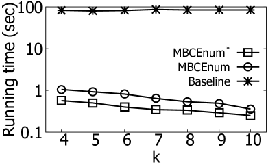
(a) $\mathsf{Slashdot}$ (vary $k$)

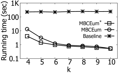
(b) $\mathsf{Epinions}$ (vary $k$)

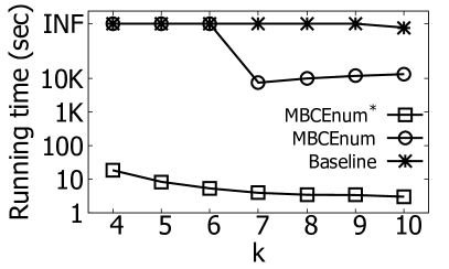
(c) $\mathsf{DBLP}$ (Vary $k$)

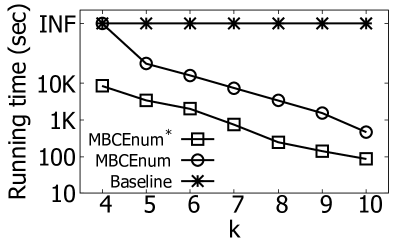
(d) $\mathsf{Douban}$ (Vary $k$)

Figure 7: Running time of $\mathsf{MBCE}$ algorithms varying $k$

Exp-1: Efficiency of $\mathsf{MBCE}$ algorithms when varying $k$. In this experiment, we evaluate the efficiency of three algorithms when varying $k$ from 4 to 10 and the results are shown in Figure 7.

As shown in Figure 7, $\mathsf{Baseline}$ consumes the most time among three algorithms on all datasets when we vary $k$ and it can only handle the small datasets. $\mathsf{MBCEnum}$ is faster than $\mathsf{Baseline}$ on most of the test cases as $\mathsf{MBCEnum}$ takes the uniqueness of the signed networks into consideration and enumerates the maximal balanced cliques based on the signed network directly. $\mathsf{MBCEnum^{*}}$ is the most efficient algorithm on all datasets when varying $k$ due to the utilization of in-enumeration optimization strategies, which reveals the effectiveness of in-enumeration optimization strategies. Another phenomena shown in Figure 7 is that the running time of all algorithms decreases as $k$ increases. This is because as $k$ increases, the pruning power of the optimization strategies proposed in Section 6 strengthens.

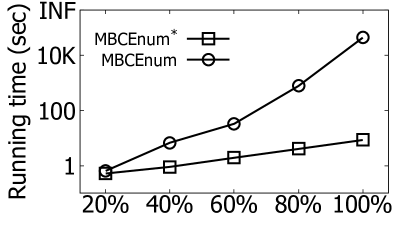
(a) $\mathsf{DBLP}$ (Vary $n$)

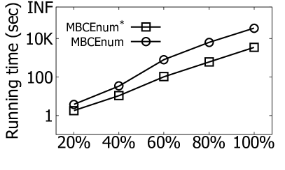
(b) $\mathsf{Douban}$ (Vary $n$)

Figure 8: Scalability of $\mathsf{MBCEnum}$ and $\mathsf{MBCEnum^{*}}$, $k$=4

Exp-2: Scalability of $\mathsf{MBCE}$ algorithms. In this experiment, we test the scalability of $\mathsf{MBCEnum}$ and $\mathsf{MBCEnum^{*}}$ on two large datasets $\mathsf{DBLP}$ and $\mathsf{Douban}$ by varying their vertices from 20% to 100%. Figure 8 shows the results.

As shown in Figure 8, when $n$ increases, the running time of both algorithms increases as well, but $\mathsf{MBCEnum^{*}}$ outperforms $\mathsf{MBCEnum}$ for all cases on both datasets. For example, on $\mathsf{DBLP}$, when we sample $20\%$ vertices, the running time of $\mathsf{MBCEnum}$ and $\mathsf{MBCEnum^{*}}$ is 0.6 seconds and 0.5 seconds, respectively, while when sampling $80\%$ vertices, their running times are 770.6 seconds and 4.0 seconds, respectively. It shows that $\mathsf{MBCEnum^{*}}$ has a good scalability in practice.

TABLE II: Case study on $\mathsf{AdjWordNet}$

$C_{L}$	$C_{R}$
raw, rough, rude	refined, smooth, suave
relaxing, reposeful, restful	restless,uneasy, ungratified, unsatisfied
interior, internal, intimate	away, foreign, outer, outside, remote
assumed, false, fictitious, fictive, mistaken, off-key, pretended, put-on, sham, sour, untrue	actual, existent, existing, factual, genuine, literal, real, tangible, touchable, true, truthful, unfeigned, veridical
active, animated, combat-ready, dynamic, dynamical, fighting, participating, alive, live	adynamic, asthenic, debilitated, enervated, undynamic, stagnant, light
following, undermentioned, next	ahead, in-the-lead, leading, preeminent, prima, star, starring, stellar
undesirable, unsuitable, unwanted	cherished, treasured, wanted, precious

Exp-3: Case study on AdjWordNet. In this experiment, we perform a case study on the real dateset $\mathsf{AdjWordNet}$. In this dataset, two synonyms have a positive edge and two antonyms have a negative edge, and Table II shows some results obtained by our algorithm. As shown in Table II, words in $C_{L}$ or $C_{R}$ have similar meaning while each word from $C_{L}$ is an antonym to all words in $C_{R}$. This case study verifies that maximal balanced clique enumeration can be applied in the applications to find synonym and antonym groups on dictionary data.

8.2 The Performance of MBCS Algorithms

Exp-4: Efficiency of $\mathsf{MBCS}$ algorithms when varying $k$. To evaluate the efficiency of $\mathsf{MBCS}$ algorithms, we record the running time of them on eight datasets, $k=[2-10]$, the results are shown at Figure 9.

As shown at Figure 9, with the value of $k$ increasing, the running time of three algorithms decreases on most datasets. For each value of $k$, $\mathsf{MBCSear}$-$\mathsf{SSP^{*}}$ is the fastest algorithm of the three algorithms, while $\mathsf{MBCSear}$ is the most time-consuming. Moreover, on large graphs as Livejournal, Orkut and Dbpedia, when $k$=2, $\mathsf{MBCSear}$ and $\mathsf{MBCSear}$-$\mathsf{SSP}$ can not get the result within a reasonable time, only $\mathsf{MBCSear}$-$\mathsf{SSP^{*}}$ can get the result. The running time of $\mathsf{MBCSear}$-$\mathsf{SSP^{*}}$ on the three graphs are 413.4s, 3626.0s and 1833.6s, respectively. It’s because that $\mathsf{MBCSear}$ has to search on the whole graph, while $\mathsf{MBCSear}$-$\mathsf{SSP}$ uses search space partition to search the maximum balanced clique within a partial subgraph. Based on $\mathsf{MBCSear}$-$\mathsf{SSP}$, benefited from multiple optimization strategies for further reducing the search space, $\mathsf{MBCSear}$-$\mathsf{SSP^{*}}$ is the most efficient algorithm of them, it can efficiently search result on all datasets.

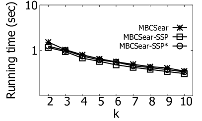
(a) $\mathsf{Slashdot}$ (Vary $k$)

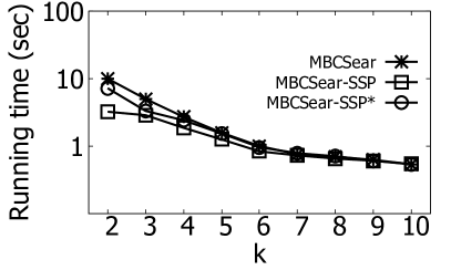
(b) $\mathsf{Epinions}$ (Vary $k$)

(c) $\mathsf{DBLP}$ (Vary $k$)

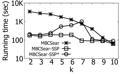
(d) $\mathsf{Douban}$ (Vary $k$)

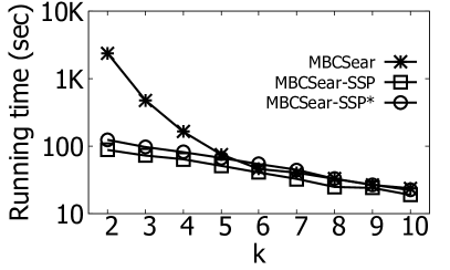
(e) $\mathsf{Pokec}$ (Vary $k$)

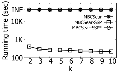
(f) Livejournal (Vary $k$)

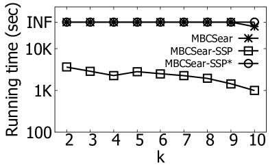
(g) $\mathsf{Orkut}$ (Vary $k$)

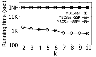
(h) Dbpedia (Vary $k$)

Figure 9: Running time of $\mathsf{MBCS}$ algorithms varying $k$

Exp-5: Effectiveness of $\mathsf{MBCS}$ algorithms when varying $k$. To intuitively compare the effectiveness of three $\mathsf{MBCS}$ algorithms, in this experiment, we record the amount of calculation of three algorithms on eight datasets, $k=[2-5]$. The calculation quantity is the time of invoking $\mathsf{MBCSearUtil}$ and $\mathsf{MBCSearUtil^{*}}$, which can intuitively represent the search space of different algorithms. The experimental results are shown at Figure 10.

As shown at Figure 10(a), when $k=2$, on all datasets, the calculation quantity of $\mathsf{MBCSear}$-$\mathsf{SSP^{*}}$ is much less than that of other algorithms. Meanwhile, $\mathsf{MBCSear}$-$\mathsf{SSP}$’s calculation quantity is less than $\mathsf{MBCSear}$’s. For instance, on DBLP(DB), the calculation quantity of $\mathsf{MBCSear}$, $\mathsf{MBCSear}$-$\mathsf{SSP}$ and $\mathsf{MBCSear}$-$\mathsf{SSP^{*}}$ are 155,621, 328 and 183, respectively. When $k>2$, the trend is similar. It’s because $\mathsf{MBCSear}$-$\mathsf{SSP^{*}}$ and $\mathsf{MBCSear}$-$\mathsf{SSP}$ are based on search space partitions, which can reduce the total search space effectively. The experimental results also confirm the reason for the efficiency of $\mathsf{MBCSear}$-$\mathsf{SSP^{*}}$ at $\mathsf{Exp}$-4.

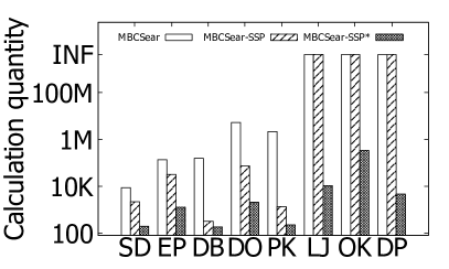
(a) $k$=2

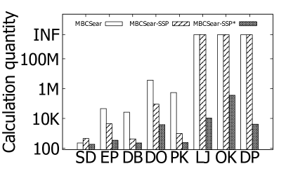
(b) $k$=3

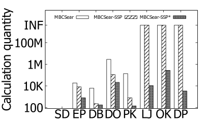
(c) $k$=4

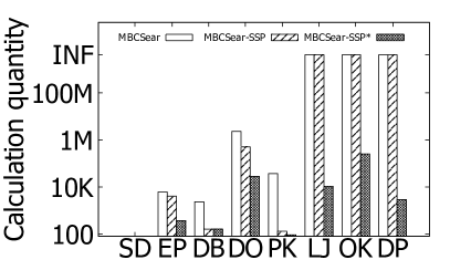
(d) $k$=5

Figure 10: Calculation quantity of different algorithms

TABLE III: The search process of $\mathsf{MBCSear}$-$\mathsf{SSP^{*}}$

Index	Search Region	$|E^{+}_{G^{\prime}}|$	$|E^{-}_{G^{\prime}}|$	$G^{\prime}/G(\%)$	$\epsilon$
0	(2,78)	0	0	0	4
1	(2,39)	0	0	0	4
2	(2,20)	21,695	12,190	0.24	33
3	(13,13)	0	0	0	33

(a) $\mathsf{MBCSear}$-$\mathsf{SSP^{*}}$ on Douban, $k$=2

Index	Search Region	$|E^{+}_{G^{\prime}}|$	$|E^{-}_{G^{\prime}}|$	$G^{\prime}/G(\%)$	$\epsilon$
0	(2,37)	0	0	0	4
1	(2,19)	6,605	2,521	0.30	29
2	(10,10)	0	0	0	29

(b) $\mathsf{MBCSear}$-$\mathsf{SSP^{*}}$ on Pokec, $k$=2

Exp-6: Search process of $\mathsf{MBCSear}$-$\mathsf{SSP^{*}}$ on real datasets. In this experiment, we show the search process of $\mathsf{MBCSear}$-$\mathsf{SSP^{*}}$ algorithm on Douban and Pokec datasets, $k$=2. Table IV(b) shows every search region $(\overline{\kappa},\underline{\kappa})$, the size of its input graph $G^{\prime}$ including positive edges number $|E^{+}_{G^{\prime}}|$ and negative edges number $|E^{-}_{G^{\prime}}|$, the ratio of $G^{\prime}$ in the original graph $G$, and the maximum balanced clique size $\epsilon$ found so far. Since Douban and Pokec are big datasets, the search process is time consuming, hence, $\mathsf{MBCSear}$-$\mathsf{SSP^{*}}$ adopts $Dec(\overline{k})=\lceil\frac{\overline{\kappa}}{2}\rceil$.

As Table IV(b) shows, on Douban, the first search region $(\underline{\kappa}_{0},\overline{\kappa}_{0})$ is $(2,78)$, and $\epsilon$ is initialized as 4. $\mathsf{MBCSear}$-$\mathsf{SSP^{*}}$ first invokes $\mathsf{EdgeReduction^{+}}$ to pre-reduce useless edges in $G$. Due to the large value of $\overline{\kappa}_{0}$, all edges are pruned from $G$. Hence, $G^{\prime}$ is empty here. For the second search region $(2,39)$, $G^{\prime}$ is still empty. For the third search region $(2,20)$, $G^{\prime}$ has 21,695 positive edges and 12,190 negative edges, it only holds 0.24% edges of the original graph which is much less than $G$. Then, $\mathsf{MBCSear}$-$\mathsf{SSP^{*}}$ finds the maximum balanced clique $C^{*}$ on $G^{\prime}$. The size of $C^{*}$ is 33. For the last search region $(13,13)$, $G^{\prime}$ is empty, the search process is finished. The search process on Pokec is similar.

By observing the search process of $\mathsf{MBCSear}$-$\mathsf{SSP^{*}}$ on the two datasets, We find two significant phenomena. First, benefited from the search space partition paradigm, the number of search regions is limited. Second, the input graph $G^{\prime}$ for each search region is much smaller than the original graph, because the edge reduction strategy can remove most of the invalid edges before the search starting.

Exp-7: Scalability of $\mathsf{MBCS}$ algorithms. In this experiment, we evaluate the scalability of $\mathsf{MBCS}$ algorithms on two biggest datasets Orkut and Dbpedia as Exp-2. The results are shown at Figure 11.

As Figure 11 shows, with the number of vertices increases, the running time of three algorithms increases as well. Among them, the growth rate of $\mathsf{MBCSear}$-$\mathsf{SSP^{*}}$ is the most stable. For instance, on Dbpedia with 40% vertices, $\mathsf{MBCSear}$ cannot get result within a reasonable time, the running time of $\mathsf{MBCSear}$-$\mathsf{SSP}$ and $\mathsf{MBCSear}$-$\mathsf{SSP^{*}}$ are 11953.0s and 319.9s, respectively. On Dbpedia with more than 40% vertices, only $\mathsf{MBCSear}$-$\mathsf{SSP^{*}}$ can get result within a reasonable time. The trend of running time on Orkut is similar. Therefore, $\mathsf{MBCSear}$-$\mathsf{SSP^{*}}$ can scale to large-scale graphs.

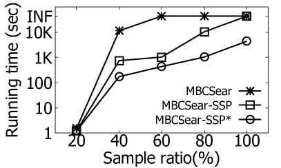
(a) Orkut (Vary $n$)

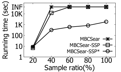
(b) Dbpedia (Vary $n$)

Figure 11: Scalability of $\mathsf{MBCS}$ algorithms, $k$=2

9 Conclusions

In this paper, we study the maximal balanced clique enumeration problem in signed networks. We propose a new enumeration algorithm tailored for signed networks. Based on the new enumeration algorithm, we explore two optimization strategies to further improve the efficiency of the enumeration algorithm. Besides, we study the maximum balanced clique search problem, and propose a novel search space partition-based search framework. Moreover, we explore multiple optimization strategies to further reduce the search space during search process. The experimental results on real datasets demonstrate the efficiency, effectiveness and scalability of our solutions.

References

- [1] D. Ouyang, L. Yuan, F. Zhang, L. Qin, and X. Lin, “Towards efficient path skyline computation in bicriteria networks,” in Proceedings of DASFAA, 2018, pp. 239–254.
- [2] L. Yuan, L. Qin, W. Zhang, L. Chang, and J. Yang, “Index-based densest clique percolation community search in networks,” IEEE TKDE, vol. 30, no. 5, pp. 922–935, 2018.
- [3] L. Yuan, L. Qin, X. Lin, L. Chang, and W. Zhang, “Effective and efficient dynamic graph coloring,” PVLDB, vol. 11, no. 3, pp. 338–351, 2017.
- [4] X. Feng, L. Chang, X. Lin, L. Qin, W. Zhang, and L. Yuan, “Distributed computing connected components with linear communication cost,” Distributed and Parallel Databases, vol. 36, no. 3, pp. 555–592, 2018.
- [5] B. Liu, L. Yuan, X. Lin, L. Qin, W. Zhang, and J. Zhou, “Efficient (, )-core computation: an index-based approach,” in Proceedings of WWW, 2019, pp. 1130–1141.
- [6] X. Wu, L. Yuan, X. Lin, S. Yang, and W. Zhang, “Towards efficient k-tripeak decomposition on large graphs,” in Proceedings of DASFAA, 2019, pp. 604–621.
- [7] Z. Qing, L. Yuan, F. Zhang, L. Qin, X. Lin, and W. Zhang, “External topological sorting in large graphs,” in Proceedings of DASFAA, 2018, pp. 203–220.
- [8] D. Ouyang, L. Yuan, L. Qin, L. Chang, and Y. Zhang, “Efficient shortest path index maintenance on dynamic road networks with theoretical guarantees,” PVLDB, vol. 13, no. 5, pp. 602–615, 2020.
- [9] J. Pattillo, N. Youssef, and S. Butenko, “On clique relaxation models in network analysis,” European Journal of Operational Research, vol. 226, no. 1, pp. 9–18, 2013.
- [10] C. Bron and J. Kerbosch, “Finding all cliques of an undirected graph (algorithm 457),” Commun. ACM, vol. 16, no. 9, pp. 575–576, 1973.
- [11] D. Eppstein, M. Löffler, and D. Strash, “Listing all maximal cliques in sparse graphs in near-optimal time,” in International Symposium on Algorithms and Computation, 2010, pp. 403–414.
- [12] D. Eppstein and D. Strash, “Listing all maximal cliques in large sparse real-world graphs,” in International Symposium on Experimental Algorithms, 2011, pp. 364–375.
- [13] L. Yuan, L. Qin, X. Lin, L. Chang, and W. Zhang, “Diversified top-k clique search,” VLDB J., vol. 25, no. 2, pp. 171–196, 2016.
- [14] D. Easley and J. Kleinberg, Networks, crowds, and markets: Reasoning about a highly connected world. Cambridge University Press, 2010.
- [15] S. Kumar, F. Spezzano, V. S. Subrahmanian, and C. Faloutsos, “Edge weight prediction in weighted signed networks,” in IEEE 16th International Conference on Data Mining, 2016, pp. 221–230.
- [16] J. Kunegis, A. Lommatzsch, and C. Bauckhage, “The slashdot zoo: mining a social network with negative edges,” in Proceedings of WWW, 2009, pp. 741–750.
- [17] J. Leskovec, D. Huttenlocher, and J. Kleinberg, “Signed networks in social media,” in Proceedings of SIGCHI, 2010, pp. 1361–1370.
- [18] L. Ou-Yang, D.-Q. Dai, and X.-F. Zhang, “Detecting protein complexes from signed protein-protein interaction networks,” IEEE/ACM Transactions on Computational Biology and Bioinformatics, vol. 12, no. 6, pp. 1333–1344, 2015.
- [19] D. Cartwright and F. Harary, “Structural balance: a generalization of heider’s theory.” Psychological review, vol. 63, no. 5, p. 277, 1956.
- [20] S. A. Marvel, S. H. Strogatz, and J. M. Kleinberg, “Energy landscape of social balance,” Physical review letters, vol. 103, no. 19, p. 198701, 2009.
- [21] P. Abell and M. Ludwig, “Structural balance: a dynamic perspective,” Journal of Mathematical Sociology, vol. 33, no. 2, pp. 129–155, 2009.
- [22] S. A. Marvel, J. Kleinberg, R. D. Kleinberg, and S. H. Strogatz, “Continuous-time model of structural balance,” Proceedings of the National Academy of Sciences, vol. 108, no. 5, pp. 1771–1776, 2011.
- [23] T. Derr, C. Aggarwal, and J. Tang, “Signed network modeling based on structural balance theory,” in Proceedings of CIKM, 2018, pp. 557–566.
- [24] F. Heider, “Attitudes and cognitive organization,” The Journal of psychology, vol. 21, no. 1, pp. 107–112, 1946.
- [25] F. Harary et al., “On the notion of balance of a signed graph.” The Michigan Mathematical Journal, vol. 2, no. 2, pp. 143–146, 1953.
- [26] L. Chang, “Efficient maximum clique computation and enumeration over large sparse graphs,” VLDB J., vol. 29, no. 5, pp. 999–1022, 2020.
- [27] C. Lu, J. X. Yu, H. Wei, and Y. Zhang, “Finding the maximum clique in massive graphs,” PVLDB, vol. 10, no. 11, pp. 1538–1549, 2017.
- [28] J. Chen, S. Cai, S. Pan, Y. Wang, Q. Lin, M. Zhao, and M. Yin, “Nuqclq: An effective local search algorithm for maximum quasi-clique problem,” in AAAI 2021, pp. 12 258–12 266.
- [29] B. Lyu, L. Qin, X. Lin, Y. Zhang, Z. Qian, and J. Zhou, “Maximum biclique search at billion scale,” Proc. VLDB Endow., vol. 13, no. 9, pp. 1359–1372, 2020.
- [30] A. Zhou, Y. Wang, and L. Chen, “Finding large diverse communities on networks: The edge maximum k*-partite clique,” Proc. VLDB Endow., vol. 13, no. 11, pp. 2576–2589, 2020. [Online]. Available: http://www.vldb.org/pvldb/vol13/p2576-zhou.pdf
- [31] E. Sevinç and T. Dökeroglu, “A novel parallel local search algorithm for the maximum vertex weight clique problem in large graphs,” Soft Comput., vol. 24, no. 5, pp. 3551–3567, 2020.
- [32] R. Li, X. Wu, H. Liu, J. Wu, and M. Yin, “An efficient local search for the maximum edge weighted clique problem,” IEEE Access, vol. 6, pp. 10 743–10 753, 2018.
- [33] X. Song, Y. Chi, K. Hino, and B. Tseng, “Identifying opinion leaders in the blogosphere,” in Proceedings of CIKM, 2007, pp. 971–974.
- [34] R. Axelrod and D. S. Bennett, “A landscape theory of aggregation,” BJPS, vol. 23, no. 02, p. 211–233, 1993.
- [35] M. Išoraitė, “Importance of strategic alliances in company’s activity,” BJPS, vol. 1, no. 5, p. 39–46, 2009.
- [36] G. A. Miller., “Wordnet: a lexical database for english,” Communications of the ACM, vol. 38, no. 11, p. 39–41, 1995.
- [37] V. Kumar, N. Joshi, A. Mukherjee, G. Ramakrishnan, and P. Jyothi, “Cross-lingual training for automatic question generation,” in ACL, 2019, pp. 4863–4872.
- [38] A. Krishnan, D. P, S. Ranu, and S. Mehta, “Leveraging semantic resources in diversified query expansion,” World Wide Web, vol. 21, no. 4, pp. 1041–1067, 2018.
- [39] X. Zheng and D. Zeng, “Social balance in signed networks,” Information Systems Frontiers, vol. 17, no. 5, pp. 1077–1095, 2015.
- [40] R.-H. Li, Q. Dai, L. Qin, G. Wang, X. Xiao, J. X. Yu, and S. Qiao, “Efficient signed clique search in signed networks,” in Proceedings of ICDE, 2018, pp. 245–256.
- [41] F. Hao, S. S. Yau, G. Min, and L. T. Yang, “Detecting k-balanced trusted cliques in signed social networks,” IEEE Internet Computing, vol. 18, no. 2, pp. 24–31, 2014.
- [42] Akkoyunlu and E. A, “The enumeration of maximal cliques of large graphs[j],” SIAM Journal on Computing, vol. 2, no. 1, pp. 1–6, 1973.
- [43] E. Tomita, A. Tanaka, and H. Takahashi, “The worst-case time complexity for generating all maximal cliques and computational experiments,” Theoretical Computer Science, vol. 363, no. 1, pp. 28–42, 2006.
- [44] F. Fakhfakh, M. Tounsi, M. Mosbah, and A. H. Kacem, “Algorithms for finding maximal and maximum cliques: A survey,” in International Conference on Intelligent Systems Design and Applications, 2017, pp. 745–754.
- [45] S. B. Seidman, “Network structure and minimum degree,” Social networks, vol. 5, no. 3, pp. 269–287, 1983.
- [46] J. Cohen, “Trusses: Cohesive subgraphs for social network analysis,” IEEE Transactions on Knowledge and Data Engineering, 2008.
- [47] X. Huang, H. Cheng, L. Qin, W. Tian, and J. X. Yu, “Querying k-truss community in large and dynamic graphs,” in SIGMOD, 2014, pp. 1311–1322.
- [48] R. Zhou, C. Liu, J. X. Yu, W. Liang, B. Chen, and J. Li, “Finding maximal k-edge-connected subgraphs from a large graph,” in EDBT, 2012.
- [49] L. Yuan, L. Qin, X. Lin, L. Chang, and W. Zhang, “I/O efficient ECC graph decomposition via graph reduction,” PVLDB, vol. 9, no. 7, pp. 516–527, 2016.
- [50] ——, “I/O efficient ECC graph decomposition via graph reduction,” VLDB J., vol. 26, no. 2, pp. 275–300, 2017.
- [51] A. E. Sariyuce, C. Seshadhri, A. Pinar, and U. V. Catalyurek, “Finding the hierarchy of dense subgraphs using nucleus decompositions,” in Proceedings of WWW, 2015, pp. 927–937.
- [52] A. E. Sariyüce, C. Seshadhri, A. Pinar, and Ü. V. Çatalyürek, “Nucleus decompositions for identifying hierarchy of dense subgraphs,” TWEB, vol. 11, no. 3, pp. 16:1–16:27, 2017.
- [53] J. Cheng, L. Zhu, Y. Ke, and S. Chu, “Fast algorithms for maximal clique enumeration with limited memory,” in Proceedings of SIGKDD, 2012, pp. 1240–1248.
- [54] M. C. Schmidt, N. F. Samatova, K. Thomas, and B.-H. Park, “A scalable, parallel algorithm for maximal clique enumeration,” J. Parallel Distrib. Comput., vol. 69, no. 4, pp. 417–428, 2009.
- [55] Y. Zhang, C. A. Phillips, G. L. Rogers, E. J. Baker, E. J. Chesler, and M. A. Langston, “On finding bicliques in bipartite graphs: a novel algorithm and its application to the integration of diverse biological data types,” BMC bioinformatics, vol. 15, no. 1, p. 110, 2014.
- [56] D. Wen, L. Qin, Y. Zhang, X. Lin, and J. X. Yu, “I/O efficient core graph decomposition: Application to degeneracy ordering,” IEEE TKDE, vol. 31, no. 1, pp. 75–90, 2019.
- [57] L. Lovász, M. E. Saks, and W. T. Trotter, “An on-line graph coloring algorithm with sublinear performance ratio,” Discret. Math., vol. 75, no. 1-3, pp. 319–325, 1989.
- [58] L. Chu, Z. Wang, J. Pei, J. Wang, Z. Zhao, and E. Chen, “Finding gangs in war from signed networks,” in Proceedings of SIGKDD, 2016, pp. 1505–1514.
- [59] T. Xu, D. Liu, E. Chen, H. Cao, and J. Tian, “Towards annotating media contents through social diffusion analysis,” in Proceedings of ICDM, 2012, pp. 1158–1163.