Convergence Rate Bounds for the Mirror Descent Method:
IQCs and the Bregman Divergence

Abstract

This paper is concerned with convergence analysis for the mirror descent (MD) method, a well-known algorithm in convex optimization. An analysis framework via integral quadratic constraints (IQCs) is constructed to analyze the convergence rate of the MD method with strongly convex objective functions in both continuous-time and discrete-time. We formulate the problem of finding convergence rates of the MD algorithms into feasibility problems of linear matrix inequalities (LMIs) in both schemes. In particular, in continuous-time, we show that the Bregman divergence function, which is commonly used as a Lyapunov function for this algorithm, is a special case of the class of Lyapunov functions associated with the Popov criterion, when the latter is applied to an appropriate reformulation of the problem. Thus, applying the Popov criterion and its combination with other IQCs, can lead to convergence rate bounds with reduced conservatism. We also illustrate via examples that the convergence rate bounds derived can be tight.

I Introduction

The mirror descent (MD) method was initially proposed by Nemirovsky and Yudin [1] for solving constrained convex optimization problems. By choosing a Bregman distance function in place of the Euclidean distance to reflect the geometry of the constraint sets, it generalizes the gradient descent (GD) method from the Euclidean space to Hilbert and Banach spaces [2]. Due to its applications in machine learning and large-scale optimization problems, it has received considerable research attention in various contexts, such as stochastic optimization [3, 4], distributed optimization [5, 6], and accelerated algorithms [7, 8].

Many optimization algorithms can be treated as nonlinear dynamical systems, whose convergence may be verified by the Lyapunov stability theorem. The Lyapunov function commonly used for the MD method is the Bregman divergence function measuring the Bregman distance between the decision variable and the optimal solution. The Bregman divergence function was introduced by Bregman to find the intersection of convex sets [9]. It has wide applications in the analysis of distributed optimization [10], port-Hamiltonian systems [11], equilibrium independent stability[12], power systems [13, 14], in addition to the MD method.

Nevertheless, when bounds on the convergence rate need to be established it is important to have systematic methods that allow to construct Lyapunov functions with more advanced structures, or allow via other means to deduce convergence rates with reduced conservatism. It has been pointed out in the optimization literature that IQCs [15] can be a useful tool in this direction [16, 17]. However, their application in the case of the MD method is non-trivial as the MD dynamics involve the composition of two nonlinearities that correspond to monotone operators, with this composition not preserving these monotonicity properties.

Our contributions in this paper can be summarized as follows:

1. We show in continuous-time that the use of the Bregman divergence as a Lyapunov function for the MD method is a special case of Lyapunov functions that follow from the Popov criterion, when this is applied to an appropriate reformulation of the problem.

2. We use conic combinations of Popov IQCs and other type of IQCs that are relevant in our reformulation to derive convergence rate bounds for the MD method with reduced conservatism.

The convergence rate bounds deduced are formulated as solutions to LMIs in both discrete and continuous time. In the case of discrete time dynamics we also show via numerical examples that these bounds can be tight.

The rest of this paper is organized as follows. In Section II, preliminaries on the MD method and IQCs are provided. The continuous-time and discrete-time MD methods are analysed via IQCs in Section III and Section IV, respectively. In Section V, numerical examples are given to verify our results. Finally, the paper is concluded in Section VI.

II Preliminaries

II-A Notation

Let $\mathbb{R}$, $\mathbb{Z}$, $\mathbb{Z}_{+}$ denote the set of real numbers, integers, and nonnegative integers, respectively. Let $I_{d}$ and $0_{d}$ denote the $d\times d$ identity matrix and zero matrix, respectively. Their subscripts can be omitted if it is clear from the context. $\textup{diag}(\alpha_{1},\ldots,\alpha_{d})$ denotes a $d\times d$ diagonal matrix with $\alpha_{i}$ on its $i$-th diagonal entry. Let $\mathbf{RH}_{\infty}$ be the set of proper real rational functions without poles in the closed right-half plane. The set of $m\times n$ matrices with elements in $\mathbf{RH}_{\infty}$ is denoted $\mathbf{RH}_{\infty}^{m\times n}$. Let $\mathbf{L}_{2}^{m}[0,\infty)$ be the Hilbert space of all square integrable and Lebesgue measurable functions $f:[0,\infty)\rightarrow\mathbb{R}^{m}$. It is a subspace of $\mathbf{L}_{2e}^{m}[0,\infty)$ whose elements only need to be integrable on finite intervals. Let ${l}_{2}^{m}(\mathbb{Z}_{+})$ be the set of all square summable sequences $f:\mathbb{Z}_{+}\rightarrow\mathbb{R}^{m}$. Given a Hermitian matrix $H(j\omega)$, $H^{*}(j\omega):=H^{T}(-j\omega)$ represents its conjugate transpose and $\text{Re}\{H(j\omega)\}$ denotes its real part.

Given $0\leq\mu\leq L$, we denote $S(\mu,L)$ as the set of functions $f:\mathbb{R}^{d}\rightarrow\mathbb{R}$ that are continuously differentiable, $\mu$-strongly convex and $L$-smooth, i.e., $\forall x,~{}y$,

$$\mu\|x-y\|^{2}\leq\left(\nabla f(x)-\nabla f(y)\right)^{T}(x-y)\leq L\|x-y\|^{2}.$$

In this work, we assume $\mu>0$ for all the functions we study if not specified otherwise. The condition number $\kappa$ of functions in $S(\mu,L)$ is defined by $\kappa:=L/\mu\geq 1$.

II-B Integral quadratic constraints

In continuous-time, a bounded operator $\Delta:\mathbf{L}_{2}^{n}[0,\infty)\rightarrow\mathbf{L}_{2}^{m}[0,\infty)$ is said to satisfy the IQC defined by $\Pi$, denoted by $\Delta\in\text{IQC}(\Pi)$, if

$$\int_{-\infty}^{\infty}\begin{bmatrix}\hat{v}(j\omega)\\ \hat{w}(j\omega)\end{bmatrix}^{*}\Pi(j\omega)\begin{bmatrix}\hat{v}(j\omega)\\ \hat{w}(j\omega)\end{bmatrix}d\omega\geq 0$$ (1)

for all $v\in\mathbf{L}_{2}^{n}[0,\infty)$ and $w=\Delta(v)$, where $\hat{v}(j\omega)$, $\hat{w}(j\omega)$ are the Fourier transforms of $v$, $w$, respectively, and $\Pi(j\omega)$ can be any measurable Hermitian valued function. In discrete-time, condition (1) is reduced to

$$\int_{-\pi}^{\pi}\begin{bmatrix}\hat{v}(e^{j\omega})\\ \hat{w}(e^{j\omega})\end{bmatrix}^{*}\Pi(e^{j\omega})\begin{bmatrix}\hat{v}(e^{j\omega})\\ \hat{w}(e^{j\omega})\end{bmatrix}d\omega\geq 0$$

for all $v\in{l}_{2}^{n}(\mathbb{Z}_{+})$, and $w=\Delta(v)$.

Define the truncation operator $P_{T}$ which does not change a function on the interval $[0,T]$ and gives the value zero on $(T,\infty]$. The operator $\Delta$ is said to be causal if $P_{T}\Delta P_{T}=P_{T}\Delta$, for all $T\geq 0$. Consider the interconnection

$$v= Gw+g$$ (2)

$$w= \Delta(v)+e$$

where $g\in\mathbf{L}_{2e}^{l}[0,\infty)$, $e\in\mathbf{L}_{2e}^{m}[0,\infty)$, $G$ and $\Delta$ are two causal operators on $\mathbf{L}_{2e}^{m}[0,\infty)$, $\mathbf{L}_{2e}^{l}[0,\infty)$, respectively. The feedback interconnection of $G$ and $\Delta$ is well-posed if the map $(v,w)\mapsto(e,g)$ defined by (2) has a causal inverse on $\mathbf{L}_{2e}^{m+l}[0,\infty)$. The interconnection is stable if, in addition, the inverse is bounded, i.e., there exists a constant $c>0$ such that $\int_{0}^{T}\left(|v|^{2}+|w|^{2}\right)dt\leq c\int_{0}^{T}\left(|g|^{2}+|e|^{2}\right)dt$. System (2) with linear $G$ and static nonlinear $\Delta$ is called a Lur’e system.

We will adopt the following IQC theorem for stability analysis.

Theorem 1 ([15]).

Let $G(s)\in\mathbf{RH}_{\infty}^{l\times m}$, and let $\Delta$ be a bounded causal operator. Assume that:

1. for every $\tau\in[0,1]$, the interconnection of $G$ and $\tau\Delta$ is well-posed;

2. for every $\tau\in[0,1]$, the IQC defined by $\Pi$ is satisfied by $\tau\Delta$;

3. there exists $\epsilon>0$ such that

   $$\begin{bmatrix}G(j\omega)\\ I\end{bmatrix}^{*}\Pi(j\omega)\begin{bmatrix}G(j\omega)\\ I\end{bmatrix}\leq-\epsilon I,~{}\forall\omega\in\mathbb{R}.$$ (3)

Then, the interconnection of $G$ and $\Delta$ is stable.

Note that if $\Pi(j\omega)=\begin{bmatrix}\Pi_{11}(j\omega)&\Pi_{12}(j\omega)\\ \Pi_{12}^{*}(j\omega)&\Pi_{22}(j\omega)\end{bmatrix}$ satisfies $\Pi_{11}(j\omega)\geq 0$ and $\Pi_{22}(j\omega)\leq 0$, then the condition $\Delta\in\text{IQC}(\Pi)$ implies that $\tau\Delta\in\text{IQC}(\Pi)$ for all $\tau\in[0,1]$.

The IQC theorem for discrete-time systems can be found in, e.g., [18].

II-C Mirror descent algorithm

Consider the optimization problem

$$\min_{x\in\mathcal{X}}f(x)$$ (4)

where $\mathcal{X}$ is a closed and convex constraint set and $\mathcal{X}\subseteq\mathbb{R}^{d}$, $f$ is the objective function and $f\in S(\mu,L)$. For simplicity, We will consider the unconstrained case in this work first, i.e., $\mathcal{X}=\mathbb{R}^{d}$, and extend the results to constraint set in the future.

We can solve (4) with the well-known gradient descent (GD) algorithm $x_{k+1}=x_{k}-\eta\nabla f(x_{k}),$ or equivalently,

$$x_{k+1}=\underset{x\in\mathbb{R}^{d}}{\text{argmin}}\left\{\nabla f(x_{k})^{T}x+\frac{1}{2\eta}\|x-x_{k}\|^{2}_{2}\right\}$$

where $\eta>0$ is a fixed stepsize. Observe that the Euclidean norm used above can be replaced with other distance measures to generate new algorithms.

The Bregman divergence defined with respect to a distance generating function (DGF) $\phi:\mathbb{R}^{d}\rightarrow\mathbb{R}$ is given by

$$D_{\phi}(y,x)=\phi(y)-\phi(x)-(y-x)^{T}\nabla\phi(x).$$ (5)

where $\phi(x)\in S(\mu_{\phi},L_{\phi})$. Then, the MD algorithm is given by

$$x_{k+1}=\underset{x\in\mathbb{R}^{d}}{\text{argmin}}\left\{\nabla f(x_{k})^{T}x+\frac{1}{\eta}D_{\phi}(x,x_{k})\right\}.$$ (6)

Denote $\bar{\phi}$ as the convex conjugate of function $\phi$, i.e.,

$$\bar{\phi}(z)=\sup_{x}\left\{x^{T}z-\phi(x)\right\}.$$

Denote $\mu_{\bar{\phi}}=L_{\phi}^{-1}$, and $L_{\bar{\phi}}=\mu_{\phi}^{-1}$. It follows that $\bar{\phi}\in S(\mu_{\bar{\phi}},L_{\bar{\phi}})$, and $z=\nabla\phi(x)\Longleftrightarrow x=\nabla\bar{\phi}(z).$ In other words, $\nabla\bar{\phi}$ is the inverse function of $\nabla\phi$. Then, the MD algorithm (6) can be written as

$$z_{k+1}=z_{k}-\eta\nabla f(x_{k}),\quad x_{k+1}=\nabla\bar{\phi}(z_{k+1})$$

or equivalently,

$$z_{k+1}=z_{k}-\eta(\nabla f\circ\nabla\bar{\phi})(z_{k})$$ (7)

where $\circ$ represents composition of functions. Similarly, the continuous MD algorithm can be given by

$$\dot{z}{(t)}=-\eta(\nabla f\circ\nabla\bar{\phi})(z{(t)}).$$ (8)

Any equilibrium point of the above systems satisfies $\nabla f\left(\nabla\bar{\phi}(z^{\text{{opt}}})\right)=\nabla f(x^{\text{{opt}}})=0_{d}$, which is the optimal solution to problem (4).

In the remainder of this paper, the time dependency in the continuous-time case will be omitted to simplify the notation.

Note that the DGF $\phi$ can be an arbitrary function in $S(\mu_{\phi},L_{\phi})$. Function $\phi$ is usually chosen such that its convex conjugate is easily computable. The principal motivation is to generate a distance function that reflects the geometry of the given constraint set $\mathcal{X}$ so that it can often be automatically eliminated during calculation. Various examples such as minimization over the unit simplex via the Kullback-Leibler divergence can be found in [19, 2, 6] and references therein.

III Continuous-time mirror descent method

In this section, we construct an IQC framework to analyze the continuous-time MD method.

III-A MD algorithm in the form of Lur’e systems

It seems that the composition of operators in (8) hinders the direct application of an IQC framework since the composite operator may not belong to the original classes of the two operators, e.g., the composition of two monotone operators is not necessarily monotone. Nevertheless, the cascade connection of two nonlinear operators can be transformed into the feedback interconnection of a linear system with the direct sum of the two nonlinear operators, similarly to the example in [15]. Therefore, the continuous-time MD algorithm (8) can be rewritten as

$$\dot{z}=Az+Bu,\quad y=Cz+Du$$ (9)

where $u=\begin{bmatrix}u_{1}\\ u_{2}\end{bmatrix}$, $y=\begin{bmatrix}y_{1}\\ y_{2}\end{bmatrix}$, the system matrices are

$$\begin{bmatrix}\begin{array}[]{c|c}A&B\\ \hline\cr C&D\end{array}\end{bmatrix}=\begin{bmatrix}\begin{array}[]{c|cc}-\eta\mu_{f}\mu_{\bar{\phi}}I_{d}&-\eta I_{d}&-\eta\mu_{f}I_{d}\\ \hline\cr\mu_{\bar{\phi}}I_{d}&0_{d}&I_{d}\\ I_{d}&0_{d}&0_{d}\end{array}\end{bmatrix}$$ (10)

and the system input is

$$\begin{bmatrix}u_{1}\\ u_{2}\end{bmatrix}= \begin{bmatrix}\nabla f(y_{1})-\mu_{f}y_{1}\\ \nabla\bar{\phi}(y_{2})-\mu_{\bar{\phi}}y_{2}\end{bmatrix}.$$ (11)

The transfer function matrix of the linear system is

$$G(s)= C(sI_{d}-A)^{-1}B+D$$ (12)

$$= \frac{1}{s+\eta\mu_{f}\mu_{\bar{\phi}}}\begin{bmatrix}-\eta\mu_{\bar{\phi}}&s\\ -\eta&-\eta\mu_{f}\end{bmatrix}\otimes I_{d}$$

where $\otimes$ denotes the Kronecker product.

Next, define $z^{\text{{opt}}}$, $x^{\text{{opt}}}$ as the optimal state with corresponding $x^{\text{{opt}}}$, $y^{\text{{opt}}}$ and $u^{\text{{opt}}}$. Let $\tilde{z}=z-z^{\text{{opt}}}$, $\tilde{y}=y-y^{\text{{opt}}}$, $\tilde{u}=u-u^{\text{{opt}}}$. We obtain the error system

$$\dot{\tilde{z}}=A\tilde{z}+B\tilde{u},\quad\tilde{y}=C\tilde{z}+D\tilde{u}$$ (13)

with

$$\begin{split}\tilde{u}:=&{\Delta}\left(\begin{bmatrix}y_{1}-y^{\text{{opt}}}_{1}\\ y_{2}-y^{\text{{opt}}}_{2}\end{bmatrix}\right)=\begin{bmatrix}\Delta_{1}\left(y_{1}-y^{\text{{opt}}}_{1}\right)\\ \Delta_{2}\left(y_{2}-y^{\text{{opt}}}_{2}\right)\end{bmatrix},\end{split}$$ (14)

where $\Delta_{1}(x)$, $\Delta_{2}(x)$ are defined by

$$\Delta_{1}(x)=\left(\nabla f(x+y_{1}^{\textup{opt}})-\mu_{f}(x+y_{1}^{\textup{opt}})\right)-\left(\nabla f(y^{\text{{opt}}}_{1})-\mu_{f}y^{\text{{opt}}}_{1}\right)$$

$$\Delta_{2}(x)=\left(\nabla\bar{\phi}(x+y_{2}^{\textup{opt}})-\mu_{\bar{\phi}}(x+y_{2}^{\textup{opt}})\right)-\left(\nabla\bar{\phi}(y^{\text{{opt}}}_{2})-\mu_{\bar{\phi}}y^{\text{{opt}}}_{2}\right).$$

It is apparent that the above error system is in the form of a Lur’e system (2), where $v=\tilde{y}$, $w=\tilde{u}$, $e=0_{d}$, and $g$ is a trajectory that represents the effect of the initial condition. The transformation can be depicted by Fig. 1.

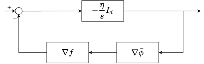
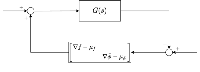
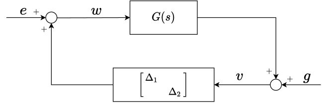
Figure 1: Transformation of the MD method to a Lur’e system. (a) represents the composition of operators, which is transformed to the direct sum of operators in (b), where $G(s)$ is given by (12). (c) is the error system in (13), and $\Delta_{1}$, $\Delta_{2}$ are given by (14).

III-B IQCs for gradients of convex functions

In this subsection, we will include a group of useful IQCs for gradients of convex functions to characterize the nonlinearity $\Delta$. Note that conic combinations of various IQCs are also valid IQCs which better characterize the nonlinearity and lead to less conservative stability margins.

III-B1 Sector IQC

The sector IQC is introduced in the following lemma as a result of the co-coercivity of gradients.

Lemma 1 ([16]).

Suppose a function $f\in S(\mu,L)$. For all $x,y$, the following quadratic constraint (QC) is satisfied,

$$\left[\begin{smallmatrix}y-x\\ \nabla{f}(y)-\nabla{f}(x)\end{smallmatrix}\right]^{T}\left[\begin{smallmatrix}-2\mu LI_{d}&(L+\mu)I_{d}\\ (L+\mu)I_{d}&-2I_{d}\end{smallmatrix}\right]\left[\begin{smallmatrix}y-x\\ \nabla{f}(y)-\nabla{f}(x)\end{smallmatrix}\right]\geq 0.$$

Note that as $f\in S(\mu_{f},L_{f})$, $\bar{\phi}\in S(\mu_{\bar{\phi}},L_{\bar{\phi}})$, then $f(\cdot)-\frac{1}{2}\mu_{f}\|\cdot\|^{2}\in S(0,L_{f}-\mu_{f})$ and $\bar{\phi}(\cdot)-\frac{1}{2}\mu_{\bar{\phi}}\|\cdot\|^{2}\in S(0,L_{\bar{\phi}}-\mu_{\bar{\phi}})$. Moreover, using Lemma 1, $\Delta\in\text{IQC}(\Pi_{s})$, where $\Delta$ is defined in (14) and

$$\Pi_{s}=\left[\begin{smallmatrix}0_{d}&0_{d}&\alpha_{1}(L_{f}-\mu_{f})I_{d}&0_{d}\\ 0_{d}&0_{d}&0_{d}&\alpha_{2}(L_{\bar{\phi}}-\mu_{\bar{\phi}})I_{d}\\ \alpha_{1}(L_{f}-\mu_{f})I_{d}&0_{d}&-2\alpha_{1}I_{d}&0_{d}\\ 0_{d}&\alpha_{2}(L_{\bar{\phi}}-\mu_{\bar{\phi}})I_{d}&0_{d}&-2\alpha_{2}I_{d}\end{smallmatrix}\right]$$ (15)

where $\alpha_{1},\alpha_{2}\geq 0$.

III-B2 Popov IQC

The Popov IQC is introduced as follows.

Lemma 2.

Suppose $f\in S(0,L)$. The nonlinearity $\nabla f(x)-\nabla f(x^{\textup{{opt}}})$ satisfies the Popov IQC by $\Pi_{P}(j\omega)$ given by

$$\Pi_{P}(j\omega)=\pm\begin{bmatrix}0_{d}&-j\omega I_{d}\\ j\omega I_{d}&0_{d}\end{bmatrix}.$$

As $f(\cdot)-\frac{1}{2}\mu_{f}\|\cdot\|^{2}\in S(0,L_{f}-\mu_{f})$ and $\bar{\phi}(\cdot)-\frac{1}{2}\mu_{\bar{\phi}}\|\cdot\|^{2}\in S(0,L_{\bar{\phi}}-\mu_{\bar{\phi}})$, using Lemma 2, we have $\Delta\in\text{IQC}(\Pi_{p}{(j\omega)})$, where $\Delta$ is defined in (14) and

$$\Pi_{p}(j\omega)=\left[\begin{smallmatrix}0_{d}&0_{d}&-j\omega\beta_{1}I_{d}&0_{d}\\ 0_{d}&0_{d}&0_{d}&-j\omega\beta_{2}I_{d}\\ j\omega\beta_{1}I_{d}&0_{d}&0_{d}&0_{d}\\ 0_{d}&j\omega\beta_{2}I_{d}&0_{d}&0_{d}\end{smallmatrix}\right]$$ (16)

where $\beta_{1},\beta_{2}\geq 0$.

III-C Convergence analysis via IQCs in frequency domain

In this subsection, we will present the convergence analysis of the MD method. There is a rich literature showing the convergence of the MD method, e.g.,[1, 19, 7]. We show that using an IQC analysis also leads to such a conclusion.

Theorem 2.

Consider a Lur’e system described by (2) where $g\in\mathbf{L}_{2}[0,\infty)$, $e\in\mathbf{L}_{2}[0,\infty)$, $G(s)$ is given by (12), $\Delta$ is defined in (14) with $f\in S(\mu_{f},L_{f})$, $\phi\in S(\mu_{\phi},L_{\phi})$. The system is stable and the trajectory of $x=\nabla\bar{\phi}(z)$ with any initial condition $z(0)=z_{0}$ of the MD method (8) converges to the optimal solution of problem (4).

Sketch of the proof. Stability can be shown using Theorem 1 with $\Pi(j\omega)$ given by

$$\Pi(j\omega)= \left[\begin{smallmatrix}0_{d}&0_{d}&\left(\alpha_{1}(L_{f}-\mu_{f})-\beta_{1}j\omega\right)I_{d}&0_{d}\\ 0_{d}&0_{d}&0_{d}&\left(\alpha_{2}(L_{\bar{\phi}}-\mu_{\bar{\phi}})-\beta_{2}j\omega\right)I_{d}\\ *&*&-2\alpha_{1}I_{d}&0_{d}\\ *&*&0_{d}&-2\alpha_{2}I_{d}\end{smallmatrix}\right].$$ (17)

Note that $\Pi(j\omega)$ of (17) is the conic combination of the sector IQC (15) and Popov IQC (16). The stability implies that $v\rightarrow 0$ as $t\rightarrow\infty$, which means the trajectories of the error system (13) tend to $0$ as $t\rightarrow\infty$ and the trajectory of $x=\nabla\bar{\phi}(z)$ for any input $z_{0}$ converges to the optimal solution of problem (4). ∎

Theorem 2 is based on conditions in the frequency domain, which do not describe the convergence rate of the MD algorithm. To this end, we will investigate, in the next subsection, the MD method in the time domain and reveal the connection between the Bregman divergence function and the Popov criterion.

III-D Convergence analysis via IQCs in time domain

In this subsection, we show that the Bregman divergence function, which is widely used as a Lyapunov function for the MD algorithm, is a special case of Lyapunov functions that are associated with the Popov criterion. This connection is established by applying the multivariable Popov criterion, which is adapted from [20, 21, 22, 23].

Lemma 3.

Let $H(s)\in\mathbf{RH}_{\infty}^{p\times p}$ and let $\psi:\mathbb{R}^{p}\to\mathbb{R}^{p}$ be a memoryless nonlinearity composed of $p$ memoryless nonlinearities $\psi_{i}$ with each being slope-restricted on sector [0, $k_{i}$], i.e., $0\leq\frac{\psi_{i}(x_{1})-\psi_{i}(x_{2})}{x_{1}-x_{2}}\leq k_{i}$, $\forall x_{1}\neq x_{2}$, $0<k_{i}\leq\infty$, for $1\leq i\leq p$. If there exist constants $\alpha_{i}\geq 0$ and $\gamma_{i}\geq 0$ such that $\text{Re}\left\{\alpha K^{-1}+(\alpha+j\omega\Gamma)H(j\omega)\right\}\geq\delta$ for some $\delta>0$, where $K=\textup{diag}(k_{1},\ldots,k_{p})$, $\alpha=\textup{diag}(\alpha_{1},\ldots,\alpha_{p})$, $\Gamma=\textup{diag}(\gamma_{1},\ldots,\gamma_{p})$. Then, the negative feedback interconnection of $H(s)$ and $\psi$ is stable.

Remark 1.

The parameters $\alpha_{i}$, $\gamma_{i}$ result directly from the conic parameterization of the sector and Popov IQCs. The proof of Theorem 2 can be seen as an application of Lemma 3 since the third condition in Theorem 1, with the IQC used in the proof of Theorem 2, is equivalent to the inequality condition in Lemma 3. It is noteworthy that the consideration of $\alpha_{i}$ is crucial since it provides more flexibility and thus less conservatice results for the MIMO case [20]. The original Popov criterion requires that the linear system $H(s)$ is strictly proper, i.e., there is no direct feedthrough term [20, 21], and the derivative of the input to $\psi$ is bounded [22]. These restrictions are removed in [23].

We can apply Lemma 3 and obtain a condition to characterize the exponential convergence rate for the continuous-time MD method.

Theorem 3.

The continuous-time MD algorithm (8) with $f\in S(\mu_{f},L_{f})$, $\phi\in S(\mu_{\phi},L_{\phi})$, converges exponentially to the optimal solution with a convergence rate $\rho$ if there exist $P>0$, $\Gamma=\textup{diag}(0,\gamma)\geq 0$, and $\alpha=\textup{diag}(\alpha_{1},\alpha_{2})\geq 0$ such that

$$\begin{bmatrix}P\tilde{A}+\tilde{A}^{T}P+2\rho P&P\tilde{B}-\tilde{C}^{T}\\ *&-\left(\tilde{D}+\tilde{D}^{T}\right)\end{bmatrix}\leq 0$$ (18)

where $\tilde{A}=A$, $\tilde{B}=-B$, $\tilde{C}={(\alpha+\rho\Gamma)}C+\Gamma CA$, $\tilde{D}=-\alpha D+\alpha K^{-1}-\Gamma CB$ and $(A,B,C,D)$ is defined in (10).

Sketch of the proof. Apply Lemma 3 with $H(s)=-G(s)$ and $\psi=\Delta$, and the Kalman-Yakubovich-Popov (KYP) Lemma[24], taking into account the exponential stability[25, Theorem 2]. ∎

The convergence rate $\rho$ in (18) needs to be treated as a constant such that (18) is an LMI. Nevertheless, a bisection search on $\rho$ can be carried out in (18) to obtain the largest admissible convergence rate for the continuous-time MD (8).

Remark 2.

Theorem 3 follows from an application of the multivariable Popov criterion and its corresponding Lyapunov function which is

$$V= \frac{1}{2}\tilde{z}^{T}P\tilde{z}+\gamma\int_{y^{\text{{opt}}}_{2}}^{y_{2}}\psi_{2}(\tau)d\tau$$ (19)

$$= \frac{1}{2}\tilde{z}^{T}P\tilde{z}+\gamma D_{\bar{\phi}}(z,z^{\text{{opt}}})-\frac{\gamma\mu_{\bar{\phi}}}{2}\|\tilde{z}\|^{2}.$$

When $P={\gamma\mu_{\bar{\phi}}I_{d}}$ and $\gamma=1$, the Lyapunov function (19) reduces to the Bregman divergence function, which is a common choice of Lyapunov function for the MD method [1, 7]. This implies that in the analysis of convergence rate, using the IQC analysis framework with a conic combination of IQCs including the Popov and Zames-Falb-O’Shea ones, yields an equivalent or less conservative worst-case convergence rate, to the one that follows by simply using the Bregman-type Lyapunov functions.

IV Discrete-time mirror descent method

Similar to the continuous-time case, the discrete-time MD algorithm in (7) can be rewritten into the following Lur’e system,

$$z_{k+1}=Az_{k}+Bu_{k},\quad y_{k}=Cz_{k}+Du_{k}$$ (20)

where $u_{k}=\begin{bmatrix}u_{k}^{(1)}\\ u_{k}^{(2)}\end{bmatrix}$, $y_{k}=\begin{bmatrix}y_{k}^{(1)}\\ y_{k}^{(2)}\end{bmatrix}$ the system matrices are

$$\begin{bmatrix}\begin{array}[]{c|c}A&B\\ \hline\cr C&D\end{array}\end{bmatrix}=\begin{bmatrix}\begin{array}[]{c|cc}(1-\eta\mu_{f}\mu_{\bar{\phi}})I_{d}&-\eta I_{d}&-\eta\mu_{f}I_{d}\\ \hline\cr\mu_{\bar{\phi}}I_{d}&0_{d}&I_{d}\\ I_{d}&0_{d}&0_{d}\end{array}\end{bmatrix}$$ (21)

and the system input is

$$\begin{bmatrix}u_{k}^{(1)}\\ u_{k}^{(2)}\end{bmatrix}= \begin{bmatrix}\nabla f(y_{k}^{(1)})-\mu_{f}y_{k}^{(1)}\\ \nabla\bar{\phi}(y_{k}^{(2)})-\mu_{\bar{\phi}}y_{k}^{(2)}\end{bmatrix}.$$ (22)

Defined $z^{\textup{{opt}}}$ as the optimal value of $z$ at steady state, with corresponding equilibrium values $y^{\textup{{opt}}}=\left(y^{(1),{\text{opt}}},y^{(2),{\textup{opt}}}\right)$, $x^{\textup{{opt}}}$, and $u^{\textup{{opt}}}$. Define $\tilde{u}_{k}=u_{k}-u^{\textup{{opt}}}$, then we have

$$\tilde{u}_{k}=\Delta\left(\begin{bmatrix}y_{k}^{(1)}-y^{(1),{\textup{opt}}}\\ y_{k}^{(2)}-y^{(2),{\textup{opt}}}\end{bmatrix}\right)$$ (23)

where the nonlinear operator $\Delta$ in (23) is the same as that used for the continuous-time algorithm in (14).

IV-A Convergence rate via IQC

There is no exact counterpart for the Popov criterion in discrete-time. Similar ones are the Jury-Lee criteria [26, 27]. Though we could easily provide an LMI condition for the discrete-time system (21), (23) following the discrete-time Jury-Lee criteria via the same Lyapunov function, we remark that in discrete-time, all IQCs to characterize monotone and bounded nonlinearities are within the set of Zames-Falb-O’Shea IQCs. Therefore, we can directly apply the class of Zames-Falb-O’Shea IQCs with a state-space representation as in [16]. We will only adopt a simple type of the Zames-Falb-O’Shea IQC here because this is sufficient to obtain a tight convergence rate for the MD method.

From [16], we can obtain that $\Delta$ satisfies the weighted-off-by-one IQC defined by $\Pi_{w}=\Psi_{w}^{*}M_{w}\Psi_{w},\quad M_{w}=\begin{bmatrix}0_{2d}&\beta I_{2d}\\ \beta I_{2d}&0_{2d}\end{bmatrix},$ where $\Psi_{w}$ is a transfer function matrix with the following state-space representation,

$$\begin{bmatrix}\begin{array}[]{c|cc}A_{\Psi_{w}}&B_{\Psi_{w}}^{y}&B_{\Psi_{w}}^{u}\\ \hline\cr C_{\Psi_{w}}&D_{\Psi_{w}}^{y}&D_{\Psi_{w}}^{u}\end{array}\end{bmatrix}=\begin{bmatrix}\begin{array}[]{c|cc}0_{2d}&-KI_{2d}&I_{2d}\\ \hline\cr\bar{\rho}^{2}I_{2d}&KI_{2d}&-I_{2d}\\ 0_{2d}&0_{2d}&I_{2d}\end{array}\end{bmatrix}$$ (24)

with $K=\textup{diag}\{L_{f}-\mu_{f},L_{\bar{\phi}}-\mu_{\bar{\phi}}\}\otimes I_{d}$, $\beta=\textup{diag}\{\beta_{1},\beta_{2}\}\otimes I_{d}\geq 0$, and $\bar{\rho}\geq 0$.

From Lemma 1, we can obtain that $\Delta$ satisfies the IQC defined by $\Pi_{s}=\Psi_{s}^{*}M_{s}\Psi_{s},\quad M_{s}=\begin{bmatrix}0_{2d}&\alpha I_{2d}\\ \alpha I_{2d}&0_{2d}\end{bmatrix},$ where $\Psi_{s}$ is a transfer function matrix with the following state-space representation,

$$\begin{bmatrix}\begin{array}[]{c|cc}A_{\Psi_{s}}&B_{\Psi_{s}}^{y}&B_{\Psi_{s}}^{u}\\ \hline\cr C_{\Psi_{s}}&D_{\Psi_{s}}^{y}&D_{\Psi_{s}}^{u}\end{array}\end{bmatrix}=\begin{bmatrix}\begin{array}[]{c|cc}0_{2d}&0_{2d}&0_{2d}\\ \hline\cr 0_{2d}&KI_{2d}&-I_{2d}\\ 0_{2d}&0_{2d}&I_{2d}\end{array}\end{bmatrix}$$ (25)

with $\alpha=\textup{diag}\{\alpha_{1},\alpha_{2}\}\otimes I_{d}\geq 0$.

Then, we can characterize the convergence rate for the discrete-time MD method by applying the discrete-time IQC theorem.

Theorem 4.

The discrete-time MD algorithm (7) with $f\in S(\mu_{f},L_{f})$ and $\phi\in S(\mu_{\phi},L_{\phi})$ converges with a rate $\bar{\rho}\leq\rho\leq 1$ if the following LMI is feasible for some $P>0$, $\alpha\geq 0$, and $\beta\geq 0$ such that

$$\left[\begin{smallmatrix}\hat{A}^{T}P\hat{A}-\rho^{2}P&\hat{A}^{T}P\hat{B}\\ *&\hat{B}^{T}P\hat{B}\end{smallmatrix}\right]+\left[\begin{smallmatrix}\hat{C}&\hat{D}\end{smallmatrix}\right]^{T}\left[\begin{smallmatrix}M_{s}&\\ &M_{w}\end{smallmatrix}\right]\left[\begin{smallmatrix}\hat{C}&\hat{D}\end{smallmatrix}\right]\leq 0$$ (26)

where

$$\hat{A}=\left[\begin{smallmatrix}A&0_{d\times 2d}&0_{d\times 2d}\\ B_{{\Psi_{s}}}^{y}C&A_{\Psi_{s}}&0_{2d\times 2d}\\ B_{{\Psi_{w}}}^{y}C&0_{2d\times 2d}&A_{\Psi_{w}}\end{smallmatrix}\right],~{}\hat{B}=\left[\begin{smallmatrix}B\\ B_{\Psi_{s}}^{y}D+B_{\Psi_{s}}^{u}\\ B_{\Psi_{w}}^{y}D+B_{\Psi_{w}}^{u}\end{smallmatrix}\right],$$

$$\hat{C}=\left[\begin{smallmatrix}D_{\Psi_{s}}^{y}C&C_{\Psi_{s}}&0_{4d\times 2d}\\ D_{\Psi_{w}}^{y}C&0_{4d\times 2d}&C_{\Psi_{w}}\end{smallmatrix}\right],~{}\hat{D}=\left[\begin{smallmatrix}D_{\Psi_{s}}^{y}D+D_{\Psi_{s}}^{u}\\ D_{\Psi_{w}}^{y}D+D_{\Psi_{w}}^{u}\end{smallmatrix}\right].$$ (27)

The proof is similar to [16, Theorem 4] and is omitted here.

IV-B Stepsize selection

It is well-known that the optimal fixed stepsize for the GD method $x_{k+1}=x_{k}-\eta\nabla f(x_{k})$ is $\eta=\frac{2}{L_{f}+\mu_{f}}$, rendering the smallest upper bound for the convergence rate $\rho=\frac{\kappa_{f}-1}{\kappa_{f}+1}$ where $\kappa_{f}=L_{f}/\mu_{f}$. Notice that the MD method has a similar structure to the GD method by changing the gradient into the composition of two functions. Thus, we let the stepsize be $\eta=\frac{2}{L_{f}L_{\bar{\phi}}+\mu_{f}\mu_{\bar{\phi}}}$ which is analogous to the optimal stepsize for the GD method. We will show numerically in Section V that the LMI in (26) is feasible for $\rho=\frac{\kappa-1}{\kappa+1}$, where $\kappa=\kappa_{f}\kappa_{\bar{\phi}}$, and $\kappa_{f}$, $\kappa_{\bar{\phi}}$ are the condition numbers of $f$, $\bar{\phi}$, respectively.

V Numerical Examples

In this section, we present two numerical examples to illustrate the IQC analysis for the MD method in continuous-time and discrete-time, respectively.

V-A Continuous-time MD method

We investigate and compare the feasibility of the IQC condition (3) when using merely the sector IQC defined by (15) and using the conic combination of the sector and Popov IQCs (17). The frequency-domain condition (3) under (15) can be easily transformed into a time-domain condition via the KYP lemma. While condition (3) under (17) is satisfied if and only if (18) in Theorem 3 is feasible for some $\rho>0$. Let $\eta=1$, $\mu_{f}=1$ and $\mu_{\bar{\phi}}=1$, and $L_{f}=L_{\bar{\phi}}$. The feasibility of the IQCs (for some $\rho>0$) with varying composite condition number $\kappa=\frac{L_{f}L_{\bar{\phi}}}{\mu_{f}\mu_{\bar{\phi}}}$ is shown in Fig. 2. Note that the MD method should converge for any $L_{f}>\mu_{f}$ and $L_{\bar{\phi}}>\mu_{\bar{\phi}}$. However, we can observe that the sector IQC defined by (15) fails to certify the convergence of the MD method for $\kappa\geq 34$. On the other hand, using the conic combination of the sector IQC (15) and the Popov IQC (16), suffices to certify its convergence for arbitrary $\kappa$.

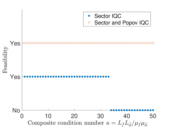
Figure 2: Feasibility of the problem using (15), the conic combination of (15) and (16), (for some $\rho>0$) with varying ratio $\kappa=\frac{L_{f}L_{\bar{\phi}}}{\mu_{f}\mu_{\bar{\phi}}}$.

V-B Discrete-time MD method

Next, we show the convergence rate for the discrete-time MD method. Let $\mu_{f}=1$, $\mu_{\bar{\phi}}=1$, and $L_{f}=L_{\bar{\phi}}$. Let the stepsize be $\eta=\frac{2}{L_{f}L_{\bar{\phi}}+\mu_{f}\mu_{\bar{\phi}}}$ as Section IV-B suggested. We compare the optimal convergence rate obtained from (26) in Theorem 4 with that obtained from the SDPs in [6], where the stepsize and convergence rate are both decision variables. The SDPs in [6] are derived from the Lyapunov function $V(z_{k})=\rho^{-k}D_{\bar{\phi}}(z_{k},z^{\textup{{opt}}})$, which is the Bregman divergence function when $\rho=1$. The relation between the composite condition number $\kappa=\frac{L_{f}L_{\bar{\phi}}}{\mu_{f}\mu_{\bar{\phi}}}$ and the convergence rate $\rho$ is shown in Fig. 3. We can observe that using the IQC analysis provides a tighter bound for the convergence rate. We remark that the convergence rate $\rho=\frac{\kappa-1}{\kappa+1}$ obtained here is tight since it is also the smallest upper bound for the convergence rates of linear systems generated by all quadratic functions $f\in S(\mu_{f},L_{f})$ and $\bar{\phi}\in S(\mu_{\bar{\phi}},L_{\bar{\phi}})$.

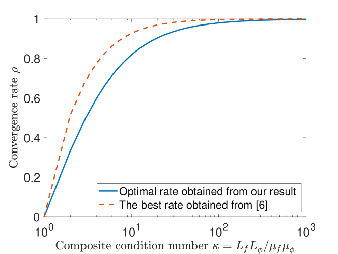
Figure 3: Convergence rate obtained from (26) in Theorem 4 and from the SDPs in [6]. The optimal rate obtained from our result coincides with the curve $\rho=\frac{\kappa-1}{\kappa+1}$.

VI Conclusion

An IQC analysis framework has been developed for the MD method in both continuous-time and discrete-time. In continuous-time, we have shown that the Bregman divergence function is a special case of the Lyapunov functions associated with the Popov criterion when these are applied to an appropriate reformulation of the problem. In discrete-time, we have provided upper bounds for the convergence rate via appropriate IQCs applied to the transformed system. It has also been illustrated via numerical examples that these bounds can be tight. Future work includes extending the framework developed to other related algorithms such as accelerated MD methods.

References

- [1] A. S. Nemirovskij and D. B. Yudin, Problem complexity and method efficiency in optimization. Wiley-Interscience, 1983.
- [2] S. Bubeck, “Convex optimization: Algorithms and complexity,” arXiv preprint arXiv:1405.4980, 2014.
- [3] J. C. Duchi, A. Agarwal, M. Johansson, and M. I. Jordan, “Ergodic mirror descent,” SIAM Journal on Optimization, vol. 22, no. 4, pp. 1549–1578, 2012.
- [4] A. Nedic and S. Lee, “On stochastic subgradient mirror-descent algorithm with weighted averaging,” SIAM Journal on Optimization, vol. 24, no. 1, pp. 84–107, 2014.
- [5] T. T. Doan, S. Bose, D. H. Nguyen, and C. L. Beck, “Convergence of the iterates in mirror descent methods,” IEEE control systems letters, vol. 3, no. 1, pp. 114–119, 2018.
- [6] Y. Sun, M. Fazlyab, and S. Shahrampour, “On centralized and distributed mirror descent: Exponential convergence analysis using quadratic constraints,” arXiv preprint arXiv:2105.14385, 2021.
- [7] W. Krichene, A. Bayen, and P. Bartlett, “Accelerated mirror descent in continuous and discrete time,” Advances in neural information processing systems, vol. 28, pp. 2845–2853, 2015.
- [8] A. Wibisono, A. C. Wilson, and M. I. Jordan, “A variational perspective on accelerated methods in optimization,” proceedings of the National Academy of Sciences, vol. 113, no. 47, pp. E7351–E7358, 2016.
- [9] L. M. Bregman, “The relaxation method of finding the common point of convex sets and its application to the solution of problems in convex programming,” USSR computational mathematics and mathematical physics, vol. 7, no. 3, pp. 200–217, 1967.
- [10] M. Li, G. Chesi, and Y. Hong, “Input-feedforward-passivity-based distributed optimization over jointly connected balanced digraphs,” IEEE Transactions on Automatic Control, 2020.
- [11] B. Jayawardhana, R. Ortega, E. Garcia-Canseco, and F. Castanos, “Passivity of nonlinear incremental systems: Application to PI stabilization of nonlinear rlc circuits,” Systems & control letters, vol. 56, no. 9-10, pp. 618–622, 2007.
- [12] J. W. Simpson-Porco, “A Hill-Moylan lemma for equilibrium-independent dissipativity,” in 2018 Annual American Control Conference (ACC). IEEE, 2018, pp. 6043–6048.
- [13] C. De Persis and N. Monshizadeh, “Bregman storage functions for microgrid control,” IEEE Transactions on Automatic Control, vol. 63, no. 1, pp. 53–68, 2017.
- [14] N. Monshizadeh and I. Lestas, “Secant and popov-like conditions in power network stability,” Automatica, vol. 101, pp. 258–268, 2019.
- [15] A. Megretski and A. Rantzer, “System analysis via integral quadratic constraints,” IEEE Transactions on Automatic Control, vol. 42, no. 6, pp. 819–830, 1997.
- [16] L. Lessard, B. Recht, and A. Packard, “Analysis and design of optimization algorithms via integral quadratic constraints,” SIAM Journal on Optimization, vol. 26, no. 1, pp. 57–95, 2016.
- [17] N. K. Dhingra, S. Z. Khong, and M. R. Jovanović, “The proximal augmented lagrangian method for nonsmooth composite optimization,” IEEE Transactions on Automatic Control, vol. 64, no. 7, pp. 2861–2868, 2018.
- [18] U. Jönsson, “Lecture notes on integral quadratic constraints,” 2001.
- [19] A. Beck and M. Teboulle, “Mirror descent and nonlinear projected subgradient methods for convex optimization,” Operations Research Letters, vol. 31, no. 3, pp. 167–175, 2003.
- [20] J. Moore and B. Anderson, “A generalization of the Popov criterion,” Journal of the franklin Institute, vol. 285, no. 6, pp. 488–492, 1968.
- [21] H. K. Khalil, “Nonlinear systems,” Prentice-Hall, New Jersey, 2002.
- [22] U. Jönsson, “Stability analysis with Popov multipliers and integral quadratic constraints,” Systems & Control Letters, vol. 31, no. 2, pp. 85–92, 1997.
- [23] J. Carrasco, W. P. Heath, and A. Lanzon, “Equivalence between classes of multipliers for slope-restricted nonlinearities,” Automatica, vol. 49, no. 6, pp. 1732–1740, 2013.
- [24] A. Rantzer, “On the Kalman–Yakubovich–Popov lemma,” Systems & Control Letters, vol. 28, no. 1, pp. 7–10, 1996.
- [25] B. Hu and P. Seiler, “Exponential decay rate conditions for uncertain linear systems using integral quadratic constraints,” IEEE Transactions on Automatic Control, vol. 61, no. 11, pp. 3631–3637, 2016.
- [26] E. Jury and B. Lee, “On the stability of a certain class of nonlinear sampled-data systems,” IEEE Transactions on Automatic Control, vol. 9, no. 1, pp. 51–61, 1964.
- [27] W. M. Haddad and D. S. Bernstein, “Parameter-dependent lyapunov functions and the discrete-time popov criterion for robust analysis,” Automatica, vol. 30, no. 6, pp. 1015–1021, 1994.