A quantum Szilard engine for two-level systems coupled to a qubit

Abstract

The innate complexity of solid state physics exposes superconducting quantum circuits to interactions with uncontrolled degrees of freedom degrading their coherence. By using a simple stabilization sequence we show that a superconducting fluxonium qubit is coupled to a two-level system (TLS) environment of unknown origin, with a relatively long energy relaxation time exceeding $50\text{\,}\mathrm{m}\mathrm{s}$. Implementing a quantum Szilard engine with an active feedback control loop allows us to decide whether the qubit heats or cools its TLS environment. The TLSs can be cooled down resulting in a four times lower qubit population, or they can be heated to manifest themselves as a negative temperature environment corresponding to a qubit population of $\sim\!$80\text{\,}\mathrm{\char 37\relax}$$. We show that the TLSs and the qubit are each other’s dominant loss mechanism and that the qubit relaxation is independent of the TLS populations. Understanding and mitigating TLS environments is therefore not only crucial to improve qubit lifetimes but also to avoid non-Markovian qubit dynamics.

Even though tremendous progress has been made to improve the coherence of superconducting qubits, they naturally have to cope with various loss and decoherence mechanisms, certainly to the chagrin of quantum computing scientists, but also to the joy of mesoscopic physicists. The relentless interactions between superconducting hardware and its environment motivate the development of quantum error correction using sophisticated stabilizer codes on the one hand [1, 2, 3, 4], and deepen our understanding of mesoscopic processes on the other hand [5, 6, 7, 8, 9, 10, 11, 12, 13, 14, 15]. These insights have motivated technologically involved strategies to mitigate decoherence from various sources, ranging from defects in dielectrics to non-thermal excitations [16]. In some cases it is even possible to manipulate two-level systems (TLSs) in the environment by applying saturation pulses [17, 18], or by performing swap operations with the qubit [19, 20]. Moreover, it has been hypothesized that using a sequence of repeated $\pi$-pulses can diffuse superconducting quasiparticles away from a qubit’s junctions [9].

Here, we present a method to manipulate and measure the environment of a quantum system via an active feedback loop implementing a quantum Szilard engine [21, 22, 23, 24]. Continuous monitoring of the qubit reveals a surprisingly long lived mesoscopic environment, which relaxes over tens of milliseconds, with the qubit providing the main dissipation channel. Conversely, this heretofore hidden environment can now be identified to be the dominant loss mechanism of our superconducting qubit, and we dread that similarly acting environments are ubiquitous in superconducting hardware. Our Szilard engine method can be applied to any quantum system that provides efficient initialization protocols via active or autonomous feedback and can directly be implemented on state of the art quantum processors [25, 26, 27]. The method can also be seen as a dynamical polarization of the environment, similar to experiments performed using spin qubits [28] and defect centers in crystals [29].

We implement the quantum Szilard engine with a granular aluminum fluxonium qubit [30, 31] that can be actively prepared in one of its eigenstates $|\text{g}\rangle$ or $|\text{e}\rangle$. The qubit interacts with a long-lived mesoscopic environment that implements the heat reservoir for the Szilard engine. The reservoir is yet of unknown physical origin, but as we shall see later, it can be modeled as a TLS ensemble. The experimental workflow, depicted in Fig. 1a, starts with a qubit stabilization sequence in either $|\text{g}\rangle$ or $|\text{e}\rangle$, thereby cooling or heating the reservoir, respectively. After stabilization, the qubit is initialized to $|\text{g}\rangle$ or $|\text{e}\rangle$ and the combined qubit and reservoir system relaxes to its steady state. As an example, in Fig. 1b we show the qubit population before and after the first preparation in a sequence stabilizing to $|\text{e}\rangle$. The amount of heat in the reservoir varies with the operation time of the Szilard engine, given by the number of qubit preparations $N$. Correspondingly, in Fig. 1c we show the measured decrease of qubit transition rates $\Gamma_{\uparrow,\downarrow}$ during stabilization in $|\text{g}\rangle$ or $|\text{e}\rangle$, respectively.

The relaxation of the reservoir can not be directly observed and has to be inferred from the qubit dynamics. While the common approach is to measure the free decay of the qubit (s. Supp. A), here we exploit the fact that the qubit readout is more than $96\text{\,}\mathrm{\char 37\relax}$ quantum non-demolishing (s. Supp. B and Ref. [32]) and we perform repeated single shot readouts, resulting in stroboscopic quantum jump traces (s. Fig. 1d). The main benefit of this method is the direct determination of the transition rates $\Gamma_{\uparrow,\downarrow}$ between the ground and excited state, which allows us to discriminate between changes in the energy relaxation rate and changes in the equilibrium population of the qubit. In Fig. 2 we show measured qubit relaxation curves for several stabilization and initialization scenarios. Note that for long enough stabilizations to the excited state ($N\geq 10^{3}$) the qubit reaches population inversion (s. bottom panel in Fig. 2c), which hints at a population inversion of the reservoir. This effect is also confirmed by the inversion of the transition rates $\Gamma_{\uparrow}>\Gamma_{\downarrow}$ shown in Fig. 3a. Consequently, for $N=10^{4}$ the preparation fidelity for the excited state is higher than for the ground state (Fig. 2a inset).

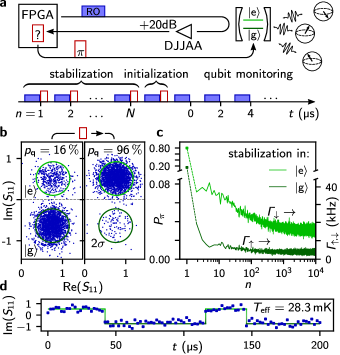
Figure 1: Szilard engine in action. a Schematic drawing of the experiment and the control sequence implementing a Szilard engine. The qubit consists of a fluxonium biased at half flux (cf. Supp. C) with its fundamental transition $f_{01}=$1.2\text{\,}\mathrm{G}\mathrm{H}\mathrm{z}$$ separated by $6.6\text{\,}\mathrm{G}\mathrm{H}\mathrm{z}$ from the higher levels. The qubit is coupled to an unknown mesoscopic environment which, as we will show in Fig. 2 and Fig. 3 can be modeled as an ensemble of TLSs. We start the experiment by stabilizing the qubit to either $|\text{g}\rangle$ or $|\text{e}\rangle$ using $N$ active feedback preparations. The stabilization is followed by a qubit initialization to $|\text{g}\rangle$ or $|\text{e}\rangle$. Finally, the qubit state is monitored stroboscopically. Throughout the sequence the qubit is measured with a repetition time $t_{\text{rep}}=$2\text{\,}\mathrm{\SIUnitSymbolMicro}\mathrm{s}$$, much shorter than the relaxation time $T_{1}\approx$20\text{\,}\mathrm{\SIUnitSymbolMicro}\mathrm{s}$$. Before we repeat the experiment we wait for $50\text{\,}\mathrm{m}\mathrm{s}$ to allow the environment to relax. The protocol is orchestrated by the field programmable gate array (FPGA) controller from Quantum Machines, with an internal real-time feedback latency of $\sim\!$200\text{\,}\mathrm{n}\mathrm{s}$$ (see Fig. S3 for a detailed setup schematics). b Scatter plot of the complex reflection coefficient $S_{11}$ of the readout signal for the qubit in equilibrium (left panel) and after $|\text{e}\rangle$-state preparation (right panel). The readout integration time is $128\text{\,}\mathrm{n}\mathrm{s}$ (Fig. 1a is not to scale) resulting in a separation of $5.6\,\sigma$ (green circles indicate $2\,\sigma$). The number of repetitions is 2500. c Probability $P_{\pi}$ for a $\pi$-pulse to be required during the stabilization. Using $t_{\text{rep}}$, the values of $p_{\pi}$ can be mapped to the qubit transition rates $\Gamma_{\uparrow}$ and $\Gamma_{\downarrow}$ for stabilization in the ground and excited state, respectively (cf. right hand axis). d Typical quantum jump trace during qubit monitoring (cf. Fig. 1a). The solid line indicates the assigned qubit state.

Figure 2: Qubit evolution after running the Szilard engine. a Measured relaxation of the qubit after being stabilized in $|\text{e}\rangle$ for various times $N\cdot t_{\text{rep}}$ followed by an initialization to either $|\text{g}\rangle$ or $|\text{e}\rangle$. Note the logarithmic $x$-axis from $300\text{\,}\mathrm{\SIUnitSymbolMicro}\mathrm{s}$ onwards, which is required to depict the slow relaxation dynamics. The exponential decay curves shown in dotted lines, with the decay times indicated by the corresponding labels, are a guide to the eye to illustrate the non-exponential relaxation of the environment (for details see Supp. E). The inset shows the preparation infidelity of the initialization. We observe an overall increasing fidelity with $N$. b Measured relaxation of the qubit after being stabilized in $|\text{g}\rangle$ followed by an initialization to either $|\text{g}\rangle$ or $|\text{e}\rangle$. Compared to panel a, the opposite effect is visible: the environment is cooled by the stabilization sequence, demonstrating that the heat flow in the environment is not the trivial result of heating due to repeated microwave readout and control pulses. The upper curves are shifted upwards by $5\text{\,}\mathrm{\char 37\relax}$ for better visibility. The continuous lines in panel a and b correspond to the theoretical model of Eqs. 1 and 2, applied to all measured curves simultaneously. c Scatter plots of the complex reflection coefficient $S_{11}$ for the relaxation curves shown in panel a for $N=10^{4}$. The left panels illustrate the reduced relaxation of the excited state population vs. time compared to Fig. 1c. The right panels demonstrate that the qubit undergoes a population inversion due to interactions with the environment. Notably, the $|\text{f}\rangle$-state is not populated, as illustrated by the absence of a third cloud in the IQ distribution (cf. Fig. S5b).

The time-evolving transition rates (Fig. 3a) are obtained from the stroboscopic quantum jump traces (Fig. 1d) by using $\Gamma_{\uparrow}=-\ln(P_{|\text{g}\rangle,|\text{g}\rangle})/t_{\text{rep}}$ and $\Gamma_{\downarrow}=-\ln(P_{|\text{e}\rangle,|\text{e}\rangle})/t_{\text{rep}}$, where $P$ is the probability to measure the same qubit state in successive measurements, and $t_{\text{rep}}$ is the repetition time. These rates define the time-dependent relaxation rate $\Gamma_{1}=\Gamma_{\uparrow}+\Gamma_{\downarrow}$ and the equilibrium population of the qubit $p_{\text{eq}}=\Gamma_{\uparrow}/\Gamma_{1}$. Note that after a heating sequence with $N=10^{4}$, $\Gamma_{1}$ of the qubit is comparably constant (Fig. 3b), while in contrast $p_{\text{eq}}$ follows a non-exponential relaxation for time scales up to $50\text{\,}\mathrm{m}\mathrm{s}$. In addition, $p_{\text{eq}}=$78\text{\,}\mathrm{\char 37\relax}$$ initially (Fig. 3c), indicating a population inversion in the reservoir. Conversely, after a cooling sequence with $N=10^{4}$, we extract $p_{\text{eq}}=$2.9\text{\,}\mathrm{\char 37\relax}$$, as can be ascertained in Fig. 2b using that the qubit population $p_{\text{q}}=$2.0\text{\,}\mathrm{\char 37\relax}$\approx p_{\text{eq}}$ after $1/\Gamma_{1}$. Hence, the Szilard engine cooled the reservoir to an effective temperature of $16\text{\,}\mathrm{m}\mathrm{K}$, which is well below the temperature of the dilution refrigerator $\sim$25\text{\,}\mathrm{m}\mathrm{K}$$ and the effective temperature $T_{\text{eff}}=$28.3\text{\,}\mathrm{m}\mathrm{K}$$ corresponding to the idle qubit population $p_{\text{th}}$ (cf. Fig. 1d).

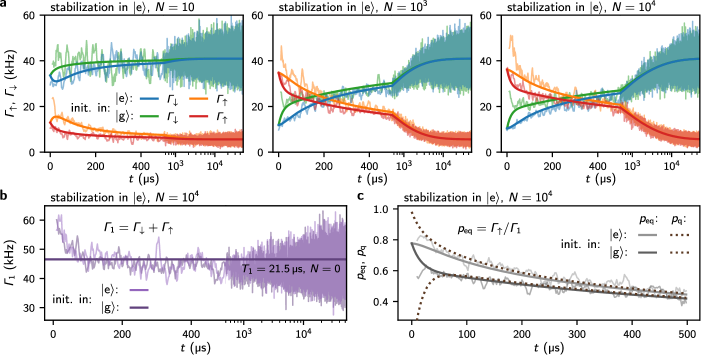
Figure 3: Signatures of the TLS environment: population inversion and constant relaxation rate. a Measured (in light color) and calculated (in dark color) transitions rates of the qubit following stabilization in $|\text{e}\rangle$ for $N=10,\,10^{3}\,\text{and}\,10^{4}$, shown in the left, center and right panel, respectively. The measured rates are extracted from the same quantum jump traces used to extract the qubit population relaxation shown in Fig. 2a. Note the logarithmic time-axis starting at $500\text{\,}\mathrm{\SIUnitSymbolMicro}\mathrm{s}$. In order to reduce the noise, a 5-point moving average filter was applied corresponding to a $10\text{\,}\mathrm{\SIUnitSymbolMicro}\mathrm{s}$ window. Furthermore, the first $10\text{\,}\mathrm{\SIUnitSymbolMicro}\mathrm{s}$ of the orange and green curve are omitted due to the low statistics; it is unlikely to have two consecutive $\lesssim$5\text{\,}\mathrm{\SIUnitSymbolMicro}\mathrm{s}$$ intervals between jumps. For long stabilization times the rates are reversed in the beginning meaning that the qubit sees a negative temperature environment. Note that the $|\text{g}\rangle$ state initialization is visibly cooling the environment, suggesting a heat capacity of only a few energy quanta. b Relaxation time $\Gamma_{1}$ obtained from the $\Gamma_{\uparrow,\downarrow}$ rates in panel a for $N=10^{4}$. The $\Gamma_{1}$ rate is constant compared to the changes in $\Gamma_{\uparrow}$ and $\Gamma_{\downarrow}$ shown in panel a, i.e. it is approximately independent of the population of the environment, which indicates a TLS environment. c Equilibrium population of the qubit $p_{\text{eq}}$ extracted from the $\Gamma_{\uparrow,\downarrow}$ rates. The dashed lines show the corresponding qubit population relaxation taken from Fig. 2a. We extrapolate an effective population of the environment $p_{\text{eq}}=$76\text{\,}\mathrm{\char 37\relax}$$ at $t=0$. In all panels, the theoretical curves use the same parameters as in Fig. 2.

The constant relaxation rate $\Gamma_{1}$ as well as the observed population inversion suggest an environment consisting of TLSs. We therefore model the system assuming the qubit is coupled to a countable number of TLSs, where each TLS with population ${p}_{\text{t}}^{k}$ has a transfer rate $\Gamma_{\text{qt}}^{k}$ with the qubit. The intrinsic relaxation rates of the qubit and the TLSs are $\Gamma_{\text{q}}$ and $\Gamma_{\text{t}}^{k}$, respectively. The rate equations read:

$$\dot{p}_{\text{q}} =-\Gamma_{\text{q}}p_{\text{q}}-\sum_{k}\Gamma_{\text{qt}}^{k}p_{\text{q}}+\sum_{k}\Gamma_{\text{qt}}^{k}p_{\text{t}}^{k}+\Gamma_{\text{q}}p_{\text{th}}\vphantom{\Big{)}}$$ (1)

$$\dot{p}_{\text{t}}^{k} =-\Gamma_{\text{t}}^{k}p_{\text{t}}^{k}-\Gamma_{\text{qt}}^{k}p_{\text{t}}^{k}+\Gamma_{\text{qt}}^{k}p_{\text{q}}+\Gamma_{\text{t}}^{k}p_{\text{th}}.\vphantom{\Big{)}}$$ (2)

Similar to Ref. [6], we use

$$\Gamma_{\text{qt}}^{k}=\frac{2g^{2}\Gamma_{\varphi}}{\Gamma_{\varphi}^{2}+\delta_{k}^{2}},$$ (3)

where $\delta_{k}$ is the detuning between the qubit and the $k^{\text{th}}$ TLS, $g$ their transverse coupling strength, and $\Gamma_{\varphi}$ the sum of their dephasing rates. Both $g$ and $\Gamma_{\varphi}$ are assumed to be identical for all TLSs. As a consequence of Eq. 2, during the stabilization time $N\cdot t_{\text{rep}}$, when we enforce $p_{\text{q}}=0\,\text{or}\,1$, there is an exponential population transfer between the qubit and each TLS, and at the end of the sequence we expect to find the TLSs in a non-thermal state, as discussed in the previous paragraph.

We solve the rate equations assuming equally spaced TLSs with $\delta_{k}=\Delta(k-c)$, where $c\in[0,0.5]$ defines a shift of the TLS ladder with respect to the qubit frequency. This allows to rewrite Eq. 3 in the simplified form $\Gamma_{\text{qt}}^{k}=a/[b^{2}+(k-c)^{2}]$ showing that $g$, $\Delta$ and $\Gamma_{\varphi}$ do not appear independently in the model. Nevertheless, from a successful fit of the model we can determine $g=\sqrt{a\Gamma_{\varphi}/2b^{2}}$ and $\Delta=\Gamma_{\varphi}/b$ for a given dephasing rate.

From a fit to the measured data we obtain $a=$5.0\text{\,}\mathrm{k}\mathrm{H}\mathrm{z}$$, $b=0.48$ and $c=0.0$ (cf. Supp. G). The robustness of the model is illustrated by the fact that a simultaneous fit of only the first $1\text{\,}\mathrm{m}\mathrm{s}$ of only two data sets (stabilization in $|\text{e}\rangle$ for $N=10^{3}$ with initialization in $|\text{g}\rangle$ or $|\text{e}\rangle$) is sufficient to describe all measurements on the entire relaxation range up to $50\text{\,}\mathrm{m}\mathrm{s}$, as demonstrated by the continuous lines in Fig. 2 and Fig. 3. For the simulation we truncate the system at 51 TLSs symmetrically spaced around the qubit frequency (with one resonant TLS).

Using the lower bound $\Gamma_{\varphi}\geq\Gamma_{\varphi}^{\text{q}}\approx$0.5\text{\,}\mathrm{M}\mathrm{H}\mathrm{z}$$, where $\Gamma_{\varphi}^{\text{q}}$ is the dephasing rate of the qubit, we extract $g\geq 2\pi\cdot$12\text{\,}\mathrm{k}\mathrm{H}\mathrm{z}$$ and $\Delta\geq 2\pi\cdot$166\text{\,}\mathrm{k}\mathrm{H}\mathrm{z}$$. The comparably small coupling strength $g\ll\Gamma_{\varphi}^{\text{q}}$ is consistent with the fact that we do not observe avoided level crossings in the qubit spectrum. Notably, this argument remains valid even for higher dephasing rates because $g$ and $\Delta$ scale with $\sqrt{\Gamma_{\varphi}}$ and $\Gamma_{\varphi}$, respectively. Using the upper bound for the dephasing rate $\Gamma_{\varphi}\sim 1/$10\text{\,}\mathrm{n}\mathrm{s}$\ll f_{\text{q}}$ gives $g<2\pi\cdot$170\text{\,}\mathrm{k}\mathrm{H}\mathrm{z}$$ and $\Delta<2\pi\cdot$35\text{\,}\mathrm{M}\mathrm{H}\mathrm{z}$$, comparable to values reported in Ref. [20].

Furthermore, using the measured qubit relaxation rate $\Gamma_{1}=\Gamma_{\text{q}}+\Gamma_{\text{qt}}^{\text{TLSs}}=1/$21.5\text{\,}\mathrm{\SIUnitSymbolMicro}\mathrm{s}$$ (Fig. 3b), we calculate its two contributions: one rate is due to interactions with the TLSs, $\Gamma_{\text{qt}}^{\text{TLSs}}=\sum_{k}\Gamma_{\text{qt}}^{k}=$35.7\text{\,}\mathrm{k}\mathrm{H}\mathrm{z}$$, and the other is the remaining intrinsic relaxation $\Gamma_{\text{q}}=$10.9\text{\,}\mathrm{k}\mathrm{H}\mathrm{z}$$. We therefore identify the TLS bath as the dominant loss mechanism. Remarkably, the fit also indicates that the intrinsic relaxation time for all TLSs exceeds $1/\Gamma_{\text{t}}\geq$50\text{\,}\mathrm{m}\mathrm{s}$$, which is orders of magnitude longer than previously measured relaxation rates of TLSs coupled to superconducting qubits [33, 34, 35]. This fact leads us to believe that we are reporting a new type of TLS environment, possibly related to trapped quasiparticle TLSs [13] or to defect centers in the materials of the superconducting qubit [36]. Finally, we would like to mention that $\Gamma_{\text{qt}}^{k}\geq\Gamma_{\text{t}}$ for $|k|\leq 15$, which means that for 31 of the TLSs the qubit is the main decay channel.

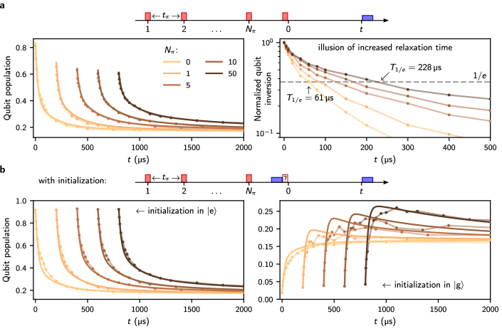
Figure S8: Heating without active feedback. a Top panel: schematic of the pulse sequence consisting of $N_{\pi}$ repeated $\pi$-pulses (red boxes) spaced by $t_{\pi}=$100\text{\,}\mathrm{\SIUnitSymbolMicro}\mathrm{s}$$, followed by a free decay measurement (the measurement pulse is indicated by the blue box). The value for $t_{\pi}$ is chosen larger than the intrinsic qubit decay time but smaller than the relaxation of the environment, in order to heat the environment. Left panel: Free decay of the qubit for various $N_{\pi}$. The curves are shifted horizontally for visibility. Right panel: Measured relaxation curves taken from the left panel, normalized and plotted in log-scale. For our device, the ostensibly increased relaxation time is an illusion, and it is explained by the increased environmental TLS population which heats the qubit, as demonstrated in panel b (right panel) and in the main text Fig. 3. Consequently, as also discussed in Supp. E, this heating of the environment forbids us to compare scaled and shifted non-exponential relaxation curves. b Top panel: schematic of the pulse sequence consisting of $N_{\pi}$ repeated $\pi$-pulses spaced by $t_{\pi}=$100\text{\,}\mathrm{\SIUnitSymbolMicro}\mathrm{s}$$, followed by an initialization to $|\text{g}\rangle$ or $|\text{e}\rangle$ immediately before the free decay measurement. Notice that this sequence is identical to the one in panel a, with the exception of the initialization pulse. The left panel measurements after initialization in $|\text{e}\rangle$ appear similar to the corresponding ones in panel a while, strikingly, after initialization to $|\text{g}\rangle$ (right panel) we observe non-monotonic evolutions of the qubit population, due to the heat stored in the TLS environment. The solid lines are simultaneous fits using the theoretical model of Eqs. 1 and 2, including the $\pi$-pulse sequence on the qubit.

Following Szilard’s seminal paper [21], the homonymous engine uses measured information as fuel (cf. Supp. H). In the first iteration of a cooling sequence starting from thermal equilibrium $T=$28.3\text{\,}\mathrm{m}\mathrm{K}$$ the engine extracts on average the internal energy $\Delta U=0.24\,k_{\text{B}}T$ from the qubit, corresponding to an entropy reduction of $0.37\,k_{\text{B}}$, which should be compared with the entropy produced by the measurement apparatus $k_{\text{B}}\ln 2\approx 0.69\,k_{\text{B}}$. From the rate equation we can calculate the optimal working regime for our Szilard engine. Using the fitted parameters we infer that the maximum heat reduction $\Delta Q=0.11\,k_{\text{B}}T$ in the reservoir occurs $68\text{\,}\mathrm{\SIUnitSymbolMicro}\mathrm{s}$ after the qubit initialization. Thus, at most half of the extracted heat from the qubit can be used to cool the reservoir. With a similar timescale of $t_{\text{rep}}=$100\text{\,}\mathrm{\SIUnitSymbolMicro}\mathrm{s}$$ we show in Fig. S8 that the reservoir can also be heated by a sequence of $\pi$-pulses. However, this procedure reminiscent of Ref. [9] can not result in a population inversion in the reservoir.

In summary, using a superconducting qubit and active feedback we demonstrated a quantum Szilard engine which can manipulate an environment of unkown origin. We can measure population inversions in both the qubit and in the environment and we show that the qubit relaxation is dominated by TLSs. Interestingly, we also show that the qubit relaxation time $T_{1}$ is unchanged by the environment population, and therefore saturating the TLS environment does not mitigate qubit relaxation. However, the qubit’s population exhibits remarkably long and non-exponential dynamics due to the intrinsically long decay time of the TLSs, exceeding $50\text{\,}\mathrm{m}\mathrm{s}$. While $T_{1}$ is independent of the environment population, the transition rates $\Gamma_{\uparrow,\downarrow}$ are not. In the context of quantum processors, where the heating and cooling of the environment is a byproduct of continuous operation, the Szilard engine could be used to symmetrize or to preferentially reduce one of the qubit transition rates. For example, reducing $\Gamma_{\uparrow}$ would be beneficial for bosonic codes [37, 38].

In our system quantum coherence between the qubit and the TLSs can be neglected, allowing a simple description using the Pauli master equation. As quantum hardware continues to improve, coherent interactions and non-Markovian qubit dynamics will start to play a role, raising the bar for quantum error correction strategies. The quantum Szilard engine presented here offers a first glimpse of the challenges facing future hardware, in which coherence improvements also translate into increasingly complex interactions with the environment.

Data availability

All relevant data are available from the authors upon reasonable request.

Supplementary material

In this supplementary material we provide further information on the relaxation measured in free decay and asses quantum demolishing efects introduced by the readout. We introduce the fluxonium qubit and the microwave setup. Furthermore, we detail on the non-exponential relaxation of the environment, show the relaxation at a higher fridge temperature ($T=$75\text{\,}\mathrm{m}\mathrm{K}$$) and discuss the relative frequency shift of the TLS ladder with respect to the qubit frequency. We also recapitulate the quantum Szilard engine and elaborate on its usage as a refrigerator. Finally, we show the heating of the reservoir without active feedback.

A Free decay of the qubit after stabilization.

In Fig. S1a we show the measured qubit free decay after stabilization in $|\text{e}\rangle$. We observe qualitatively the same behavior as in Fig. 2a in the main text, which was measured with quantum jumps. The whole set of experiments including the four stabilization and initialization scenarios each with various $N$ values lasts for approximately $20\text{\,}\mathrm{h}$ and can be affected by drifts in the environment, as illustrated in Fig. S1b.

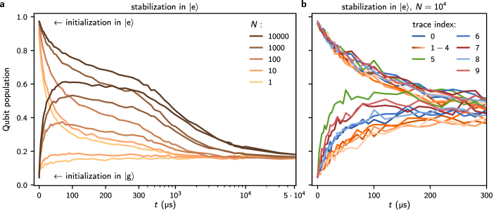
Figure S1: Measured free decay after stabilization in $|\text{e}\rangle$. a Free decay of the qubit after stabilization for various times $N\cdot t_{\text{rep}}$ followed by an initialization to either $|\text{g}\rangle$ or $|\text{e}\rangle$. Similarly to Fig. 2a in the main text, the qubit reaches a population inversion of approximately $60\text{\,}\mathrm{\char 37\relax}$ after being initialized in $|\text{g}\rangle$. b We observe fluctuations at the beginning of the relaxation curves after stabilization in $|\text{e}\rangle$, especially for initialization in $|\text{g}\rangle$. The color coding is used to indicate quantitatively different time evolutions, which can be grouped in at least four families (blue, orange, green and red), suggesting at least four different configurations of the TLS environment. Following Eq. 3, the main contributions can be expected from the most resonant TLSs that affect in particular the beginning of the relaxation curves. A corresponding behaviour for each trace index is also observed for the curves after stabilization in $|\text{g}\rangle$, which are measured interleaved (not shown), in which case the fluctuations are mainly seen for the initialization in $|\text{e}\rangle$. The data set shown in the left panel was selected to be one of the few without fluctuations. The time interval between measurements with successive indices is $2\text{\,}\mathrm{h}$. These random fluctuations are also present in data obtained from quantum jumps. Nevertheless, since the data acquisition time is more than ten times faster for quantum jumps experiments, it is less likely to observe such fluctuations. This allows us to fit simultaneously the data sets for stabilization in $|\text{g}\rangle$ and $|\text{e}\rangle$ for several values of $N$, as shown by the continuous lines in main text Fig. 2 and Fig. 3.

B Qubit relaxation as a function of the readout repetition time

First, we discuss the influence of the measurement on the qubit relaxation for which we contrast different $T_{1}$-experiments in Fig. S2a. The measurement increases both transition rates $\Gamma_{\uparrow,\downarrow}$ compared to the free decay rates (Fig. S2d). However, for the relaxation rate $\Gamma_{1}=\Gamma_{\uparrow}+\Gamma_{\downarrow}$ the $\Gamma_{\downarrow}$-rate contributes dominantly. For a repetition time $t_{\text{rep}}=$2\text{\,}\mathrm{\SIUnitSymbolMicro}\mathrm{s}$$, the additional rate $\Gamma_{\downarrow}^{\text{M}}\approx$20\text{\,}\mathrm{k}\mathrm{H}\mathrm{z}$$ induced by the measurement corresponds to a probability of approximately $4\text{\,}\mathrm{\char 37\relax}$ per measurement to decay from the excited state. The relative increase of $\Gamma_{\downarrow}$ exceeds the one of $\Gamma_{\uparrow}$ and therefore lowers the qubit’s effective temperature compared to free decay (s. Fig. S2b).

Second, we illustrate the challenges in measuring the relaxation rate of a qubit coupled to a finite TLS environment. From the quantum jumps analysis, we obtain $T_{1}=$21.4\pm 2.2\text{\,}\mathrm{\SIUnitSymbolMicro}\mathrm{s}$$ for $t_{\text{rep}}=$2\text{\,}\mathrm{\SIUnitSymbolMicro}\mathrm{s}$$ (as reported in the main text). In contrast, an exponential fit to the data shown in Fig. S2a results in higher $T_{1}$ values even though we conservatively use only the first $20\text{\,}\mathrm{\SIUnitSymbolMicro}\mathrm{s}$ for the fit (Fig. S2c). This discrepancy is a consequence of the finite size of the TLS environment. The energy transferred into the environment by the initial qubit $\pi$-pulse is sufficient to create the illusion of an increased relaxation time (cf. Fig. S8a right panel). The difference illustrates the importance of the quantum jump method for measuring the energy relaxation. However, when $t_{\text{rep}}$ approaches $T_{1}$ the equilibrium population $p_{\text{eq}}$ is not constant in between successive measurements. In this regime, the quantum jumps method also overestimates the relaxation time, as visible in Fig. S2c where the quantum jumps method approaches the free decay $T_{1}$-time extracted from the exponential fit for $t_{\text{rep}}=$20\text{\,}\mathrm{\SIUnitSymbolMicro}\mathrm{s}$$.

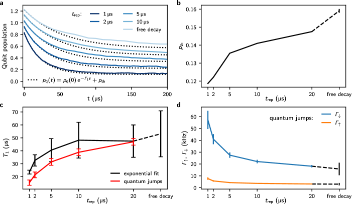
Figure S2: Quantum demolition effects induced by the readout. a Qubit relaxation obtained from quantum jump traces for various repetition times $t_{\text{rep}}$ and from free decay. The curves are successively shifted vertically by $10\text{\,}\mathrm{\char 37\relax}$ for visibility. The deviation from the exponential function, especially close to the thermal equilibrium, is an indication that the TLS reservoir was heated by the energy deposited in the qubit during the initial $\pi$-pulse (cf. Fig. S8). b The shift of the thermal qubit population $p_{\text{th}}$ to lower values with decreasing repetition time indicates a cooling effect of the measurement on the qubit. When not visible the error bars are in the range of the line width. c Relaxation times $T_{1}$ extracted either from exponential fits to the data in panel a or from quantum jumps. For the exponential fits we use the first $20\text{\,}\mathrm{\SIUnitSymbolMicro}\mathrm{s}$ of the decay together with the baseline $p_{\text{th}}$ (panel b) to extract the $T_{1}$ values (for the deviation see discussion in the text). In both cases we observe shorter $T_{1}$ values at faster repetition times, indicating the increasing quantum demolition contribution to the energy relaxation budget. The results reported in the main text were measured with $t_{\text{rep}}=$2\text{\,}\mathrm{\SIUnitSymbolMicro}\mathrm{s}$$, for which approximately half of the relaxation can be attributed to the quantum demolishing of the readout. d Measured qubit transition rates extracted from quantum jump traces for various $t_{\text{rep}}$. The quantum demolishing of the readout mainly consists in an increased $\Gamma_{\downarrow}$-rate. In all panels the lines connecting the points are guides to the eye.

C The fluxonium artificial atom

The device under study is a fluxonium artificial atom that can be measured by the dispersive frequency shift of its inductively coupled readout resonator. Both the fluxonium circuit and the resonator exploit the high kinetic inductance of granular aluminum. Details about the device can be found in Ref. [32] and in the supplementary material of Ref. [31]. The Josephson junction of the fluxonium is realized with a superconducting quantum interference device (SQUID) to have a flux tunable Josephson energy. In the following, we discuss the fluxonium Hamiltonian and point out two consequences that emerge from the SQUID implementation. For a time-independent external flux bias the Hamiltonian can be transformed to read

$$H =\frac{1}{2C}\,q^{2}+\frac{1}{2L}\,\phi^{2}-E_{\text{J}_{1}}\cos\left(\frac{2\pi}{\Phi_{0}}\left(\phi-\Phi_{\text{ext}}^{\text{l}}\right)\right)\,-\,E_{\text{J}_{2}}\cos\left(\frac{2\pi}{\Phi_{0}}\left(\phi-\Phi_{\text{ext}}^{\text{l}}-\Phi_{\text{ext}}^{\text{s}}\right)\right),$$ (S1)

where $q$ and $\phi$ are the charge and flux operators obeying the commutation relation $[q,\phi]=i\hbar$. The capacitance $C=$6.9\text{\,}\mathrm{f}\mathrm{F}$$ is mainly formed by the capacitances of the Josephson junctions of the SQUID. The kinetic superinductance $L=$231\text{\,}\mathrm{n}\mathrm{H}$$ and the inner Josephson junction with the Josephson energy $E_{\text{J}_{1}}$ enclose the external flux $\Phi_{\text{ext}}^{\text{l}}$. The second Josephson junction with the Josephson energy $E_{\text{J}_{2}}$ encloses an additional flux $\Phi_{\text{ext}}^{\text{s}}$ with the first junction, the external flux of the SQUID. Introducing the dimensionless flux variable $\varphi$, the flux-dependent Josephson energies in Eq. S1 can be rewritten as

$$E_{\text{J}_{1}}\cos (\varphi-\varphi_{\text{l}})\,+\,E_{\text{J}_{2}}\cos(\varphi-(\varphi_{\text{l}}+\varphi_{\text{s}}))$$

$$=\text{sign}\left(E_{\Sigma}\left(\varphi_{\text{s}}\right)\right)\cdot\sqrt{E_{\Sigma}\left(\varphi_{\text{s}}\right)^{2}+E_{\Delta}\left(\varphi_{\text{s}}\right)^{2}}\,\cdot\,\cos\left(\varphi-\varphi_{\text{ext}}-\arctan\left(\frac{E_{\Delta}\left(\varphi_{\text{s}}\right)}{E_{\Sigma}\left(\varphi_{\text{s}}\right)}\right)\right)$$

$$=E_{\text{J}}^{\text{eff}}(\varphi_{\text{s}})\cdot\cos\left(\varphi-\varphi_{\text{ext}}^{\text{eff}}(\varphi_{\text{l}},\varphi_{\text{s}})\right),$$

where the flux dependent energies are $E_{\Sigma}\left(\varphi_{\text{s}}\right)=(E_{\text{J}_{1}}+E_{\text{J}_{2}})\cos\left(\varphi_{\text{s}}/2\right)$ and $E_{\Delta}\left(\varphi_{\text{s}}\right)=(E_{\text{J}_{2}}-E_{\text{J}_{1}})\sin\left(\varphi_{\text{s}}/2\right)$ and the external flux is defined by $\varphi_{\text{ext}}=\varphi_{\text{l}}+\varphi_{\text{s}}/2$, showing that the SQUID flux contributes half to the external flux bias of the fluxonium. The resulting fluxonium Hamiltonian has an effective Josephson energy $E_{\text{J}}^{\text{eff}}$ that only depends on the external flux in the SQUID loop and is flux biased by $\varphi_{\text{ext}}^{\text{eff}}$, which includes a nonlinear phase shift term that can directly be seen in the spectrum (s. Fig. 1b in Ref. [32] or Fig. S2 in Ref. [31]). The device was operated at $\Phi_{\text{ext}}=21.48\,\Phi_{0}$ giving $E_{\text{J}}^{\text{eff}}=$5.6\text{\,}\mathrm{G}\mathrm{H}\mathrm{z}$$ and $\varphi_{\text{ext}}^{\text{eff}}/2\pi=0.5$.

The SQUID junction design comes with two implications. First, the tunable Josephson energy is susceptible to local flux noise, which in the case of our device constitutes the main decoherence mechanism. Second, the condition for destructive quasiparticle interference at the Josephson junction that decouples the qubit from quasiparticle interactions [8, 15], is not met in our device.

In order to meet the quasiparticle destructive interference condition for both junctions in a SQUID fluxonium, the device needs to be operated with half-flux bias in the fluxonium loop and integer flux bias in the SQUID loop. Under this condition, the Josephson energy terms in Eq. S1 can simply be added and the fluxonium is biased at half flux. In our case the external flux is applied globally, the enclosed fluxes $\Phi_{\text{ext}}^{\text{l}}$ and $\Phi_{\text{ext}}^{\text{s}}$ are linked by their corresponding loop areas. Defining the ratio $V=A_{\text{l}}/A_{\text{s}}$, the quasiparticle destructive interference condition requires

$$\varphi_{\text{s}}=2\pi m\quad \wedge\quad\varphi_{\text{l}}=V\varphi_{\text{s}}=2\pi mV=2\pi k-\pi,\qquad\text{with}\quad m,k\in\mathbb{Z},$$

which implies

$$V=\frac{2k-1}{2m}\,\notin\mathbb{Z}.$$

In other words, the ratio $V$ should not be an integer. Our device was designed with $V=50.0\pm 0.1$ so the quasiparticle destructive interference condition is not met at any feasible flux bias. At $\Phi_{\text{ext}}=21.48\,\Phi_{0}$, which is the flux bias used for the main text data, we have

$$\begin{array}[]{rcccr}\varphi_{\text{s}}&=&\dfrac{2}{2V+1}\,\cdot\,\varphi_{\text{ext}}&=&0.42\cdot 2\pi,\\[8.0pt] \varphi_{\text{l}}&=&\left(1-\dfrac{1}{2V+1}\right)\,\cdot\,\varphi_{\text{ext}}&=&21.27\cdot 2\pi,\\[9.0pt] \varphi_{\text{l}}+\varphi_{\text{s}}&=&\left(1+\dfrac{1}{2V+1}\right)\,\cdot\,\varphi_{\text{ext}}&=&21.69\cdot 2\pi.\end{array}$$

D The time-domain setup

In Fig. S3 we show a schematic of the microwave electronics setup for the fluxonium measurement and manipulation.

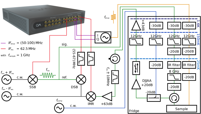
Figure S3: Experimental setup for qubit state measurements and active feedback. The experimental workflow is orchestrated by the OPX instrument from Quantum Machines (visible in the top-left photograph). This FPGA-based instrument can be programmed to measure and estimate in real-time the qubit state using the $IQ$-demodulated readout signal, and it can trigger a $\pi$-pulse in order to prepare the qubit in its target state. For the readout of the qubit, we use a $128\text{\,}\mathrm{n}\mathrm{s}$ long square pulse and an interferometric setup to purify the two-channel microwave generators that operate in continuous wave (c.w.) mode. The signal and the reference are interfered computationally by the OPX to extract the $I$ and $Q$ quadratures. We keep the intermediate frequency (IF) of the readout fixed at $62.5\text{\,}\mathrm{M}\mathrm{H}\mathrm{z}$ yielding 16 samples per period for the integration. The channels use different frequencies to account for the mixers operating on opposite sidebands. For the qubit manipulation, we use a Gaussian envelope pulse with $\sigma=$48\text{\,}\mathrm{n}\mathrm{s}$$ in a $256\text{\,}\mathrm{n}\mathrm{s}$ window. Fridge setup: All microwave lines going into the cryostat are attenuated and filtered. A home made infrared (IR) filter employing Stycast^® ensures an attenuation of more than $-10\text{\,}\mathrm{dB}$ for frequencies larger than $60\text{\,}\mathrm{GHz}$. On the way back the readout signal is first amplified with a home-made Dimer Josephson Junction Array Amplifier (DJJAA [39] providing $+$20\text{\,}\mathrm{d}\mathrm{B}$$ of gain). We feed the pump tone for the DJJAA to the readout line with a directional coupler providing minimal loss for the readout signal. After the DJJAA the readout signal passes a $40\text{\,}\mathrm{d}\mathrm{B}$ isolation before it is further amplified by a high-electron-mobility transistor (HEMT). At room temperature the readout signal is routed through a home-made tunable filter in order to suppress the DJJAA pump tone, after which it is further amplified, down-converted to the intermediate frequency and finally recorded.

E Relaxation of the environment

The equilibrium population of the qubit $p_{\text{eq}}$ is the effective population of its environment. In our case it can be measured in two ways. The first method consists in calculating $p_{\text{eq}}=\Gamma_{\uparrow}/\Gamma_{1}$ with $\Gamma_{1}=\Gamma_{\uparrow}+\Gamma_{\downarrow}$ from the qubit transition rates that can be extracted from quantum jump traces, as described in the main text and shown in Fig. 3c. The second method uses the fact that in our case the intrinsic qubit decay is orders of magnitude faster than the relaxation of the TLS environment. Therefore, the tail of the qubit relaxation, i.e. the data shown in Fig. S4, can directly be ascribed to the effective population of the TLS environment: $p_{\text{eq}}\approx p_{\text{q}}$ (see brown and grey curves in Fig. 3c). The advantage of the latter approach is its superior signal-to-noise ratio.

In Fig. S4a we plot the same measured $p_{\text{q}}$ data as in Fig. 2a in the main text using a linear time axis instead of the logarithmic axis, in order to highlight the slow non-exponential relaxation. At this point, one might still imagine that the relaxation curves $p_{\text{eq}}(t)$ are given by the time evolution of a differential equation $\dot{p}_{\text{eq}}=f(p_{\text{eq}})$, where $f$ is not simply proportional to $p_{\text{eq}}$ (exponential decay) but is an arbitrary function, e.q. similarly to Ref. [40]. In order to rule out this idea, we plot in Fig. S4b the relaxation tails from Fig. S4a shifted in time such that they start at the same population (indicated by the arrow labels). Clearly, as the derivatives of the relaxation curves differ from each other, the relaxation dynamics can not be described by a first order differential equation of the form $\dot{p}_{\text{eq}}=f(p_{\text{eq}})$. Hence, the relaxation must contain hidden variables, i.e. the TLS populations ${p}_{\text{t}}^{k}$, that we capture by the system of linear differential equations Eqs. 1 and 2. In general, the equilibrium qubit population $p_{\text{eq}}$ is defined by $\dot{p_{q}}=0$ and from Eq. 1 we have:

$$p_{\text{eq}}(t) =\frac{\Gamma_{\uparrow}(t)}{\Gamma_{1}}=\left(\sum_{k}\Gamma_{\text{qt}}^{k}p_{\text{t}}^{k}(t)+\Gamma_{\text{q}}p_{\text{th}}\right)/\,\Gamma_{1}.$$

Consequently, the nonlinear relaxation of the environment originates from the sum over the TLS populations ${p}_{\text{t}}^{k}(t)$ that itself are a sum of the $(n+1)$ exponential solutions of the linear rate equations describing the $n$ TLSs and the qubit. This gives an intuition for the fact that the measured non-exponential relaxation can only be reproduced with a large number of TLSs (more than 15). With an increasing number of TLSs, the agreement improves and the model converges. For all calculations we truncate the model at 51 TLSs.

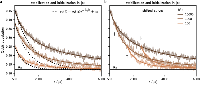
Figure S4: Relaxation of the environment. a Relaxation to thermal equilibrium plotted for $t$ starting from $500\text{\,}\mathrm{\SIUnitSymbolMicro}\mathrm{s}$, which is an order of magnitude larger than the qubit $T_{1}$. For comparison, the dotted traces in black show exponential decays which start by matching the measured decay and highlight the slow non-exponential relaxation of the environment at longer time-scales. Notice that we plot the same data as in Fig. 2a in the main text using a linear time axis. The solid lines show the calculated qubit populations using the same model and fit parameters as in the main text. b The relaxation tails from panel a shifted in time such that they start at the same qubit population (indicated by the arrow labels). Notice that the initial derivatives differ from each other, highlighting the existence of a memory (hidden variables) in the environment (see discussion in the text).

F Relaxation of the qubit at $\mathit{\mathbf{T}}=$ 75 mK

The relaxation curves shown in the main text (Fig. 1ab) were measured at a fridge temperature $T=\!$25\text{\,}\mathrm{m}\mathrm{K}$$. Here, we show measurements at $T=\!$75\text{\,}\mathrm{m}\mathrm{K}$$ in order to improve the visibility of the cooling effect.

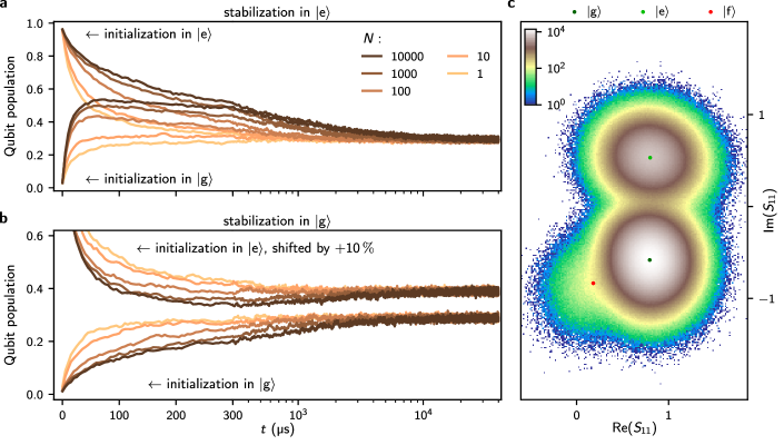
Figure S5: Relaxation measurements at $\mathit{\mathbf{T}}=$ 75 mK. a Qubit relaxation after being stabilized in $|\text{e}\rangle$ for various times $N\cdot t_{\text{rep}}$ followed by an initialization to $|\text{g}\rangle$ or $|\text{e}\rangle$. b Qubit relaxation after being stabilized in $|\text{g}\rangle$ followed by an initialization to $|\text{g}\rangle$ or $|\text{e}\rangle$. Note that at $75\text{\,}\mathrm{m}\mathrm{K}$ the final thermal population is higher, therefore increasing the visibility of the cooling effect in comparison to the main text (cf. Fig. 2b). The curves corresponding to initialization in $|\text{e}\rangle$ are shifted upwards by $10\text{\,}\mathrm{\char 37\relax}$ for better visibility. For the stroboscopic qubit monitoring the repetition time was set to $t_{\text{rep}}=$5\text{\,}\mathrm{\SIUnitSymbolMicro}\mathrm{s}$$ in order to decrease the quantum demolition effects (s. Fig. S2) c Histogram of the complex reflection coefficient $S_{\text{11}}$ acquired from the last $1\text{\,}\mathrm{m}\mathrm{s}$ of the relaxation curves shown in panel a and b. For the thermal populations of the states $|\text{g}\rangle$, $|\text{e}\rangle$ and $|\text{f}\rangle$ we expect $(67.7,\leavevmode\nobreak\ 31.9,\leavevmode\nobreak\ \text{and}\leavevmode\nobreak\ 0.4)\,$\mathrm{\char 37\relax}$$ and we measure $(70.6\pm 0.2,\leavevmode\nobreak\ 28.8,\leavevmode\nobreak\ \text{and}\leavevmode\nobreak\ 0.4\pm 0.2)\,$\mathrm{\char 37\relax}$$. For $|g\rangle$ and $|\text{e}\rangle$ the discrepancy is likely due to quantum demolition effects caused by the readout (s. Fig. S2). The populations are obtained from a Gaussian mixture model fit to the $S_{11}$ distribution using the scikit-learn library [41].

G Relative frequency shift of the TLS ladder with respect to the qubit frequency.

In Fig. S6, we show the theoretical modeling of the qubit relaxation and compare the two extreme cases of the relative frequency shift of the TLS ladder with respect to the qubit frequency. The relative frequency shift of the TLS ladder $\delta_{k}=\Delta(k-c)$ is defined by the parameter $c\in[0,0.5]$. We obtain a better description of the experimental findings for $c=0$, which corresponds to the case of having one TLS in resonance with the qubit. For $c=0$ the fit reveals $a=$5.0\text{\,}\mathrm{k}\mathrm{H}\mathrm{z}$$ and $b=0.48$, which furthermore yields $\Gamma_{\text{q}}=$10.9\text{\,}\mathrm{k}\mathrm{H}\mathrm{z}$$. In contrast, for $c=0.5$ we obtain $a=$6.6\text{\,}\mathrm{k}\mathrm{H}\mathrm{z}$$, $b=0.56$ and $\Gamma_{\text{q}}=$12.5\text{\,}\mathrm{k}\mathrm{H}\mathrm{z}$$.

Overall, it is important to note that the parameter $c$ mainly influences the beginning of the relaxation curves, since the rates of the TLSs close to the qubit frequency are predominantly affected. In reality the TLS configuration (frequencies, coupling strength, dephasing, etc.) is probably more complex than our model, we therefore find it remarkable that the even the detailed features in the beginning of the relaxation curve can be described using only three parameters. Furhtermore, the configuration of the TLSs can also change in time, even with the sample maintained at cryogenic temperatures, as illustrated in Fig. S1b.

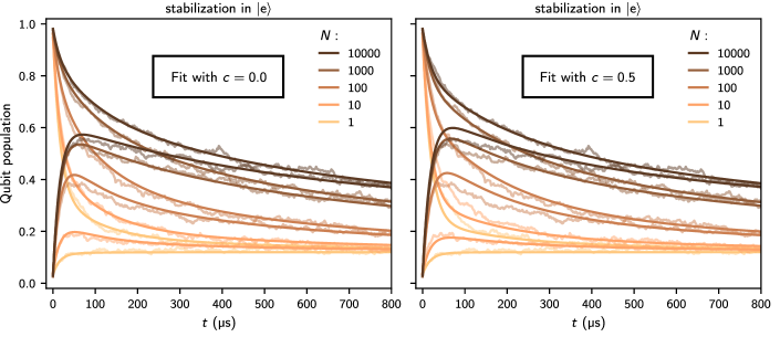
Figure S6: Relative frequency shift of the TLS ladder with respect to the qubit frequency. Comparison of the theoretical model (continuous lines) given by Eqs. 1 and 2 and using the TLS ladder introduced in the main text. For the fit we use $c=0.0$ in the left panel and $c=0.5$ in the right panel. In both panels we show in light color the same measured data as in Fig. 2a in the main text. We conclude that $c=0$ gives a better fit result by comparing the measured and calculated qubit populations in the region $t\approx$100\text{\,}\mathrm{\SIUnitSymbolMicro}\mathrm{s}$$.

H The Szilard engine

For sake of completeness, we briefly discuss the thermodynamic properties of the Szilard engine focusing on its usage as a refrigerator. The whole thermodynamic system and the refrigeration cycle are depicted in Fig. S7. Following Szilard [21], we consider a system consisting of a ground state and an excited state with a $d$-fold degeneracy. For $d=1$ we have the experimental situation where the system can be referred to as the qubit. The system’s internal energy $U$ and entropy $S$ read:

$$U=\frac{d\epsilon}{d+e^{\beta\epsilon}}\quad\text{and}\quad S/k_{\text{B}}=(S_{\text{rev}}+S_{\text{irr}})/k_{\text{B}}=\beta U+\ln\left(d+e^{\beta\epsilon}\right)-\beta\epsilon,$$

where $\epsilon$ is the energy spacing between the two system states, $\beta=1/k_{\text{B}}T$ encodes the temperature $T$ of the system and $k_{\text{B}}$ is the Boltzmann constant. The entropy can be divided into two components. The reversible entropy $S_{\text{rev}}$ can be exchanged with the TLS reservoir, while the irreversible entropy $S_{\text{irr}}$ can only increase during a thermodynamic process and is closely related to the free energy $F=TS_{\text{irr}}$ of the system.

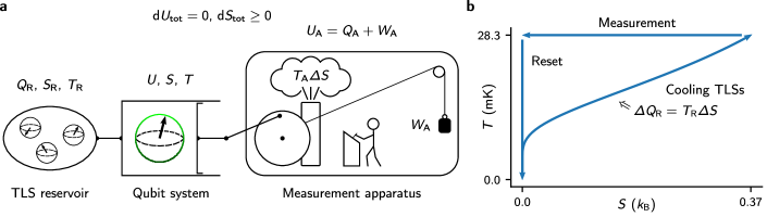
Figure S7: The Szilard engine. a Sketch of the whole thermodynamic system consisting of the measurement apparatus, the qubit and the TLS reservoir. For a closed system the internal energy is constant while the entropy can only increase irreversibly according to the second law of thermodynamics. The measurement and the feedback is performed by the intelligent being, as conceived by Szilard [21]. b Refrigeration cycle of the Szilard engine cooling the TLS reservoir.

When the system is measured quantum mechanically with an operator that collapses the system state either to its ground or excited state manifold, the entropy reduces, depending on the measurement outcome, to $S/k_{\text{B}}=0$ or $S/k_{\text{B}}=\ln d$, respectively. The maximum average entropy reduction of $\Delta S/k_{\text{B}}=\ln 2$ is attained when $\beta\epsilon=\ln d$. For the qubit, where $d=1$, this value is only reached in the limit of an infinite temperature or a vanishing energy level splitting [42].

As we consider the measurement apparatus to be a thermodynamic engine, the entropy reduction has to be compensated so that the second law of thermodynamics remains valid. Consequently, the apparatus must be connected to a heat bath to which it can unload at least the reduced entropy. When this bath is at the temperature $T_{\text{A}}$, the measurement requires the minimum work $W_{\text{M}}=T_{\text{A}}\Delta S$. Furthermore, one can argue that the measurement process should not depend on the temperature of the system. Thus, $W_{\text{M}}\geq k_{\text{B}}T_{\text{A}}\ln 2$ must hold, as was first conjectured by Szilard. For the performance consideration of the refrigerator we will drop this assumption and use the exact entropy reduction to allow for a simple comparison with the theoretical maximum performance given by the Carnot cycle.

After the measurement, the information on the system state can be used to cool down the TLS reservoir in which case the system has to be reset to its ground state. Here, we need an additional discussion for systems with a degenerate excited state. When the system is measured in the excited state manifold it cannot simply be reset to its ground state as it would mean to destroy the remaining entropy $S/k_{\text{B}}=\ln d$. Instead, additional measurements are required to determine the exact state of the system allowing to select the correct gate operations bringing the system to its ground state. Alternatively, one could think of a more powerful measurement that can distinguish between all $(d+1)$-states. This measurement, however, can produce a maximum average entropy reduction of $\Delta S/k_{\text{B}}=\ln(d+1)$ in the limit $\beta\epsilon\rightarrow 0$, in accordance with the previously mentioned limit for the qubit.

Despite, these technical details concerning the reset of the degenerate excited state to its ground state, the whole thermodynamic cycle can be summarized in three steps:

1. The measurement requires the work $W_{\text{M}}=T_{\text{A}}\Delta S$.

2. From the reset of the qubit one can in principle extract the work $W_{\text{Q}}=-\Delta U$.

3. The reservoir is cooled by the amount $\Delta Q_{\text{R}}=T_{\text{R}}\Delta S_{\text{rev}}=\Delta U$. Here, we assume that the TLS reservoir is large enough so that its temperature $T_{\text{R}}$ stays approximately constant.

The coefficient of performance (COP) now reads:

$$\text{COP}=\frac{\Delta Q_{\text{R}}}{W_{\text{tot}}}=\frac{T_{\text{R}}\Delta S_{\text{rev}}}{T_{\text{A}}(\Delta S_{\text{rev}}+\Delta S_{\text{irr}})-T_{\text{R}}\Delta S_{\text{rev}}}=\frac{T_{\text{R}}}{T_{\text{A}}-T_{\text{R}}+T_{\text{A}}\frac{\Delta S_{\text{irr}}}{\Delta S_{\text{rev}}}},$$

showing that the Szilard engine will always operate below the maximum theoretical efficiency, which is only reached in the following limit:

$$\frac{\Delta S_{\text{irr}}}{\Delta S_{\text{rev}}}=\frac{d+e^{\beta\epsilon}}{d}\left(\frac{\ln\left(d+e^{\beta\epsilon}\right)}{\beta\epsilon}-1\right)=0+\mathcal{O}\left(\frac{1}{\beta\epsilon}\right)\quad\text{for}\quad\beta\epsilon\rightarrow\infty,$$

while in contrast the cooling power given by $\Delta U$ vanishes exponentially.

In our experiment, the reservoir can be cooled at most by $\Delta Q_{\text{R}}\approx 0.5\Delta U$ as stated in the main text. This surprisingly small value seems to be in conflict with the TLS bath beeing the dominant loss mechanism $\Gamma_{\text{qt}}^{\text{TLSs}}\approx 3.3\Gamma_{\text{q}}$. This discrepancy can simply be explained by the finite size of the reservoir. The qubit only interacts strongly with the few most resonant TLSs. Consequently, when the qubit is reset to its ground state the temperature of these TLSs will reduce and the qubit can not reach its prior energy, thus $\Delta Q_{\text{R}}<\Delta U(T_{\text{R}})$.

I Heating without active feedback

Here, we show that the reservoir can be heated by a sequence of $\pi$-pulses. Our results resemble those reported in Ref. [9], however, at least for our qubit the seemingly increased $T_{1}$-time is simply due to the heated environment. Despite the similarities, the environments probed in the two experiments are not necessarily of the same nature.

References

- Ofek et al. [2016] N. Ofek, A. Petrenko, R. Heeres, P. Reinhold, Z. Leghtas, B. Vlastakis, Y. Liu, L. Frunzio, S. M. Girvin, L. Jiang, M. Mirrahimi, M. H. Devoret, and R. J. Schoelkopf, Extending the lifetime of a quantum bit with error correction in superconducting circuits, Nature 536, 441 (2016).
- Vuillot et al. [2019] C. Vuillot, H. Asasi, Y. Wang, L. P. Pryadko, and B. M. Terhal, Quantum error correction with the toric Gottesman-Kitaev-Preskill code, Phys. Rev. A 99, 032344 (2019).
- Google Quantum AI [2021] Google Quantum AI, Exponential suppression of bit or phase errors with cyclic error correction, Nature 595, 383 (2021).
- Cai et al. [2021] W. Cai, Y. Ma, W. Wang, C.-L. Zou, and L. Sun, Bosonic quantum error correction codes in superconducting quantum circuits, Fundamental Research 1, 50 (2021).
- Grabovskij et al. [2012] G. J. Grabovskij, T. Peichl, J. Lisenfeld, G. Weiss, and A. V. Ustinov, Strain tuning of individual atomic tunneling systems detected by a superconducting qubit, Science (2012).
- Barends et al. [2013] R. Barends, J. Kelly, A. Megrant, D. Sank, E. Jeffrey, Y. Chen, Y. Yin, B. Chiaro, J. Mutus, C. Neill, P. O’Malley, P. Roushan, J. Wenner, T. C. White, A. N. Cleland, and J. M. Martinis, Coherent Josephson qubit suitable for scalable quantum integrated circuits, Phys. Rev. Lett. 111, 080502 (2013).
- Ristè et al. [2013] D. Ristè, C. C. Bultink, M. J. Tiggelman, R. N. Schouten, K. W. Lehnert, and L. DiCarlo, Millisecond charge-parity fluctuations and induced decoherence in a superconducting transmon qubit, Nature Communications 4, 1913 (2013).
- Pop et al. [2014] I. M. Pop, K. Geerlings, G. Catelani, R. J. Schoelkopf, L. I. Glazman, and M. H. Devoret, Coherent suppression of electromagnetic dissipation due to superconducting quasiparticles, Nature 508, 369 (2014).
- Gustavsson et al. [2016] S. Gustavsson, F. Yan, G. Catelani, J. Bylander, A. Kamal, J. Birenbaum, D. Hover, D. Rosenberg, G. Samach, A. P. Sears, S. J. Weber, J. L. Yoder, J. Clarke, A. J. Kerman, F. Yoshihara, Y. Nakamura, T. P. Orlando, and W. D. Oliver, Suppressing relaxation in superconducting qubits by quasiparticle pumping, Science 354, 1573 (2016).
- Grünhaupt et al. [2018] L. Grünhaupt, N. Maleeva, S. T. Skacel, M. Calvo, F. Levy-Bertrand, A. V. Ustinov, H. Rotzinger, A. Monfardini, G. Catelani, and I. M. Pop, Loss mechanisms and quasiparticle dynamics in superconducting microwave resonators made of thin-film granular aluminum, Phys. Rev. Lett. 121, 117001 (2018).
- Serniak et al. [2018] K. Serniak, M. Hays, G. de Lange, S. Diamond, S. Shankar, L. D. Burkhart, L. Frunzio, M. Houzet, and M. H. Devoret, Hot nonequilibrium quasiparticles in transmon qubits, Phys. Rev. Lett. 121, 157701 (2018).
- Chu et al. [2018] Y. Chu, P. Kharel, T. Yoon, L. Frunzio, P. T. Rakich, and R. J. Schoelkopf, Creation and control of multi-phonon Fock states in a bulk acoustic-wave resonator, Nature 563, 666 (2018).
- de Graaf et al. [2020] S. E. de Graaf, L. Faoro, L. B. Ioffe, S. Mahashabde, J. J. Burnett, T. Lindström, S. E. Kubatkin, A. V. Danilov, and A. Y. Tzalenchuk, Two-level systems in superconducting quantum devices due to trapped quasiparticles, Science Advances 6, eabc5055 (2020).
- Wilen et al. [2021] C. D. Wilen, S. Abdullah, N. A. Kurinsky, C. Stanford, L. Cardani, G. D’Imperio, C. Tomei, L. Faoro, L. B. Ioffe, C. H. Liu, A. Opremcak, B. G. Christensen, J. L. DuBois, and R. McDermott, Correlated charge noise and relaxation errors in superconducting qubits, Nature 594, 369 (2021).
- Glazman and Catelani [2021] L. I. Glazman and G. Catelani, Bogoliubov quasiparticles in superconducting qubits, SciPost Phys. Lect. Notes , 31 (2021).
- Siddiqi [2021] I. Siddiqi, Engineering high-coherence superconducting qubits, Nat. Rev. Mater. 6, 875 (2021).
- Kirsh et al. [2017] N. Kirsh, E. Svetitsky, A. L. Burin, M. Schechter, and N. Katz, Revealing the nonlinear response of a tunneling two-level system ensemble using coupled modes, Phys. Rev. Mater. 1, 012601 (2017).
- Andersson et al. [2021] G. Andersson, A. L. O. Bilobran, M. Scigliuzzo, M. M. de Lima, J. H. Cole, and P. Delsing, Acoustic spectral hole-burning in a two-level system ensemble, npj Quantum Inf. 7, 1 (2021).
- Wang et al. [2013] Z. L. Wang, Y. P. Zhong, L. J. He, H. Wang, J. M. Martinis, A. N. Cleland, and Q. W. Xie, Quantum state characterization of a fast tunable superconducting resonator, Appl. Phys. Lett. 102, 163503 (2013).
- Lisenfeld et al. [2019] J. Lisenfeld, A. Bilmes, A. Megrant, R. Barends, J. Kelly, P. Klimov, G. Weiss, J. M. Martinis, and A. V. Ustinov, Electric field spectroscopy of material defects in transmon qubits, npj Quantum Information 5, 105 (2019).
- Szilard [1929] L. Szilard, Über die Entropieverminderung in einem thermodynamischen System bei Eingriffen intelligenter Wesen, Zeitschrift für Physik 53, 840 (1929).
- Toyabe et al. [2010] S. Toyabe, T. Sagawa, M. Ueda, E. Muneyuki, and M. Sano, Experimental demonstration of information-to-energy conversion and validation of the generalized Jarzynski equality, Nature Physics 6, 988 (2010).
- Koski et al. [2014] J. V. Koski, V. F. Maisi, J. P. Pekola, and D. V. Averin, Experimental realization of a Szilard engine with a single electron, Proceedings of the National Academy of Sciences 111, 13786 (2014).
- Peterson et al. [2020] J. P. S. Peterson, R. S. Sarthour, and R. Laflamme, Implementation of a quantum engine fuelled by information (2020), arXiv:2006.10136 [quant-ph] .
- Córcoles et al. [2021] A. D. Córcoles, M. Takita, K. Inoue, S. Lekuch, Z. K. Minev, J. M. Chow, and J. M. Gambetta, Exploiting dynamic quantum circuits in a quantum algorithm with superconducting qubits, Phys. Rev. Lett. 127, 100501 (2021).
- Gold et al. [2021] A. Gold, J. P. Paquette, A. Stockklauser, M. J. Reagor, M. S. Alam, A. Bestwick, N. Didier, A. Nersisyan, F. Oruc, A. Razavi, B. Scharmann, E. A. Sete, B. Sur, D. Venturelli, C. J. Winkleblack, F. Wudarski, M. Harburn, and C. Rigetti, Entanglement across separate silicon dies in a modular superconducting qubit device, npj Quantum Inf. 7, 1 (2021).
- Satzinger et al. [2021] K. J. Satzinger, Y.-J. Liu, A. Smith, C. Knapp, M. Newman, C. Jones, Z. Chen, C. Quintana, X. Mi, A. Dunsworth, C. Gidney, I. Aleiner, F. Arute, K. Arya, J. Atalaya, R. Babbush, J. C. Bardin, R. Barends, J. Basso, A. Bengtsson, A. Bilmes, M. Broughton, B. B. Buckley, D. A. Buell, B. Burkett, N. Bushnell, B. Chiaro, R. Collins, W. Courtney, S. Demura, A. R. Derk, D. Eppens, C. Erickson, L. Faoro, E. Farhi, A. G. Fowler, B. Foxen, M. Giustina, A. Greene, J. A. Gross, M. P. Harrigan, S. D. Harrington, J. Hilton, S. Hong, T. Huang, W. J. Huggins, L. B. Ioffe, S. V. Isakov, E. Jeffrey, Z. Jiang, D. Kafri, K. Kechedzhi, T. Khattar, S. Kim, P. V. Klimov, A. N. Korotkov, F. Kostritsa, D. Landhuis, P. Laptev, A. Locharla, E. Lucero, O. Martin, J. R. McClean, M. McEwen, K. C. Miao, M. Mohseni, S. Montazeri, W. Mruczkiewicz, J. Mutus, O. Naaman, M. Neeley, C. Neill, M. Y. Niu, T. E. O’Brien, A. Opremcak, B. Pató, A. Petukhov, N. C. Rubin, D. Sank, V. Shvarts, D. Strain, M. Szalay, B. Villalonga, T. C. White, Z. Yao, P. Yeh, J. Yoo, A. Zalcman, H. Neven, S. Boixo, A. Megrant, Y. Chen, J. Kelly, V. Smelyanskiy, A. Kitaev, M. Knap, F. Pollmann, and P. Roushan, Realizing topologically ordered states on a quantum processor, Science (2021).
- Bluhm et al. [2010] H. Bluhm, S. Foletti, D. Mahalu, V. Umansky, and A. Yacoby, Enhancing the coherence of a spin qubit by operating it as a feedback loop that controls its nuclear spin bath, Phys. Rev. Lett. 105, 216803 (2010).
- London et al. [2013] P. London, J. Scheuer, J.-M. Cai, I. Schwarz, A. Retzker, M. B. Plenio, M. Katagiri, T. Teraji, S. Koizumi, J. Isoya, R. Fischer, L. P. McGuinness, B. Naydenov, and F. Jelezko, Detecting and polarizing nuclear spins with double resonance on a single electron spin, Phys. Rev. Lett. 111, 067601 (2013).
- Manucharyan et al. [2009] V. E. Manucharyan, J. Koch, L. I. Glazman, and M. H. Devoret, Fluxonium: Single cooper-pair circuit free of charge offsets, Science 326, 113 (2009).
- Grünhaupt et al. [2019] L. Grünhaupt, M. Spiecker, D. Gusenkova, N. Maleeva, S. T. Skacel, I. Takmakov, F. Valenti, P. Winkel, H. Rotzinger, W. Wernsdorfer, A. V. Ustinov, and I. M. Pop, Granular aluminium as a superconducting material for high-impedance quantum circuits, Nature Materials 18, 816 (2019).
- Gusenkova et al. [2021] D. Gusenkova, M. Spiecker, R. Gebauer, M. Willsch, D. Willsch, F. Valenti, N. Karcher, L. Grünhaupt, I. Takmakov, P. Winkel, D. Rieger, A. V. Ustinov, N. Roch, W. Wernsdorfer, K. Michielsen, O. Sander, and I. M. Pop, Quantum nondemolition dispersive readout of a superconducting artificial atom using large photon numbers, Phys. Rev. Applied 15, 064030 (2021).
- Neeley et al. [2008] M. Neeley, M. Ansmann, R. C. Bialczak, M. Hofheinz, N. Katz, E. Lucero, A. O’Connell, H. Wang, A. N. Cleland, and J. M. Martinis, Process tomography of quantum memory in a Josephson-phase qubit coupled to a two-level state, Nature Physics 4, 523 (2008).
- Lisenfeld et al. [2010] J. Lisenfeld, C. Müller, J. H. Cole, P. Bushev, A. Lukashenko, A. Shnirman, and A. V. Ustinov, Measuring the temperature dependence of individual two-level systems by direct coherent control, Phys. Rev. Lett. 105, 230504 (2010).
- Lisenfeld et al. [2016] J. Lisenfeld, A. Bilmes, S. Matityahu, S. Zanker, M. Marthaler, M. Schechter, G. Schön, A. Shnirman, G. Weiss, and A. V. Ustinov, Decoherence spectroscopy with individual two-level tunneling defects, Scientific Reports 6, 23786 (2016).
- Yang et al. [2020] F. Yang, T. Gozlinski, T. Storbeck, L. Grünhaupt, I. M. Pop, and W. Wulfhekel, Microscopic charging and in-gap states in superconducting granular aluminum, Phys. Rev. B 102, 104502 (2020).
- Reinhold et al. [2020] P. Reinhold, S. Rosenblum, W.-L. Ma, L. Frunzio, L. Jiang, and R. J. Schoelkopf, Error-corrected gates on an encoded qubit, Nat. Phys. 16, 822 (2020).
- Grimm et al. [2020] A. Grimm, N. E. Frattini, S. Puri, S. O. Mundhada, S. Touzard, M. Mirrahimi, S. M. Girvin, S. Shankar, and M. H. Devoret, Stabilization and operation of a Kerr-cat qubit, Nature 584, 205 (2020).
- Winkel et al. [2020] P. Winkel, I. Takmakov, D. Rieger, L. Planat, W. Hasch-Guichard, L. Grünhaupt, N. Maleeva, F. Foroughi, F. Henriques, K. Borisov, J. Ferrero, A. V. Ustinov, W. Wernsdorfer, N. Roch, and I. M. Pop, Nondegenerate parametric amplifiers based on dispersion-engineered Josephson-junction arrays, Phys. Rev. Appl. 13, 024015 (2020).
- Wang et al. [2014] C. Wang, Y. Y. Gao, I. M. Pop, U. Vool, C. Axline, T. Brecht, R. W. Heeres, L. Frunzio, M. H. Devoret, G. Catelani, L. I. Glazman, and R. J. Schoelkopf, Measurement and control of quasiparticle dynamics in a superconducting qubit, Nature Communications 5, 5836 (2014).
- Pedregosa et al. [2011] F. Pedregosa, G. Varoquaux, A. Gramfort, V. Michel, B. Thirion, O. Grisel, M. Blondel, P. Prettenhofer, R. Weiss, V. Dubourg, J. Vanderplas, A. Passos, D. Cournapeau, M. Brucher, M. Perrot, and E. Duchesnay, Scikit-learn: Machine learning in Python, Journal of Machine Learning Research 12, 2825 (2011).
- Pekola et al. [2016] J. P. Pekola, D. S. Golubev, and D. V. Averin, Maxwell’s demon based on a single qubit, Phys. Rev. B 93, 024501 (2016).