Nonlinear interactions of dipolar excitons and polaritons in MoS₂ bilayers

Nonlinear interactions between excitons strongly coupled to light are key for accessing quantum many-body phenomena in polariton systems[1, 2, 3, 4, 5]. Atomically-thin two-dimensional semiconductors provide an attractive platform for strong light-matter coupling owing to many controllable excitonic degrees of freedom[6, 7, 8, 9, 10]. Among these, the recently emerged exciton hybridization opens access to unexplored excitonic species [11, 12, 13, 14, 15], with a promise of enhanced interactions[16]. Here, we employ hybridized interlayer excitons (hIX) in bilayer MoS₂ [11, 12, 13, 14] to achieve highly nonlinear excitonic and polaritonic effects. Such interlayer excitons possess an out-of-plane electric dipole [12] as well as an unusually large oscillator strength [11] allowing observation of dipolar polaritons (dipolaritons [17, 18, 19]) in bilayers in optical microcavities. Compared to excitons and polaritons in MoS₂ monolayers, both hIX and dipolaritons exhibit $\approx 8$ times higher nonlinearity, which is further strongly enhanced when hIX and intralayer excitons, sharing the same valence band, are excited simultaneously. This gives rise to a highly nonlinear regime which we describe theoretically by introducing a concept of hole crowding. The presented insight into many-body interactions provides new tools for accessing few-polariton quantum correlations [20, 21, 22].

Excitons in two-dimensional transition metal dichalcogenides (TMDs) have large oscillator strengths and binding energies [23], making them attractive as a platform for studies of strong light-matter coupling in optical microcavities [6, 7, 8, 9]. A variety of polaritonic states have been realised using monolayers of MX₂ (M=Mo, W; X=S, Se) embedded in tunable [7, 9, 10, 24] and monolithic microcavities [25, 26, 27, 16, 28].

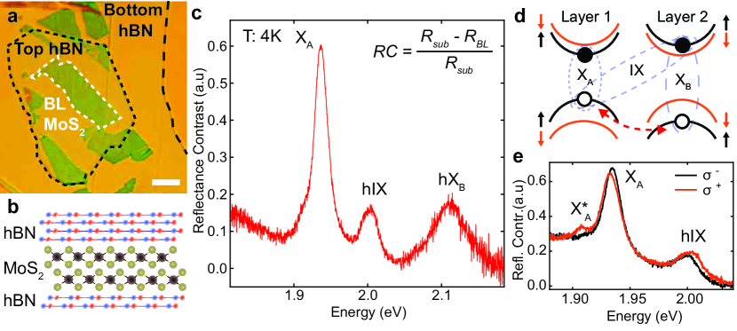
Figure 1: Homobilayer MoS₂ and its optical response. a, Bright field microscope image of an encapsulated BL MoS₂ transferred on top of a DBR. Scale bar: 10 $\mu$m. b, Schematic side-view of the fabricated heterostructure comprising a BL MoS₂ sandwiched between few-layer hBN. c, Reflectance contrast (RC) spectrum of the sample measured at low temperature (4 K) showing three distinct absorption features at 1.937 eV, 2.004 eV and 2.113 eV for X_A, hIX and hX_B, respectively. The measured linewidths for X_A, hIX, and hX_B are $20$, $23$ and $64$ meV, respectively. RC is calculated using the formula in the top-right corner of the graph. d, Sketch of the conduction and valence bands in two adjacent layers of MoS₂, displaying the allowed optical transitions of A and B direct intralayer excitons (X_A and X_B) and interlayer excitons (IX) for spin-up states (black lines) at the K point in the bilayer momentum space. IX hybridizes with X_B through the hole tunnelling between the two layers (red dashed arrow). At the K’ point of the bilayer Brillouin zone, the same configuration applies for the states with the opposite spins. e, RC spectra of excitons in BL MoS₂ detected in two circular polarizations in an out-of-plane magnetic field of 8 T at $T$=4 K. Zeeman shifts of opposite signs are observed for X_A and hIX. The absorption peak of the charged intralayer exciton (X${}^{*}_{A}$) shows near unity circular polarization.

One of the central research themes in polaritonics is the study of nonlinear interactions leading to extremely rich phenomena such as Bose-Einstein condensation [1, 2], polariton lasing [3, 4] or optical parametric amplification [5]. Polaritons formed from tightly bound neutral intralayer excitons in TMDs are not expected to show strong nonlinearity. However, pronounced nonlinear behavior was observed for trion polaritons [29, 24] and Rydberg polaritons [30]. Enhanced nonlinearity can be achieved by employing excitonic states with a physically separated electron and hole, e.g. in adjacent atomic layers [31] or quantum wells [32, 19, 33, 17, 18]. Such interlayer excitons have a large out-of-plane electric dipole moment, and thus can strongly mutually interact [34]. Typically, however, interlayer or ’spatially indirect’ excitons possess low oscillator strength [31, 35]. Thus, in order to strongly couple to cavity photons, hybridization with high-oscillator-strength intralayer excitons is required [17, 18, 19, 36, 16].

An attractive approach for realization of dipolar excitons and polaritons is to employ the recently discovered exciton hybridization in MoS₂ bilayers [11, 37]. This approach allows realization of uniform samples suitable for the observation of macroscopic many-body phenomena [38]. Interlayer excitons unique to bilayer MoS₂ possess a large oscillator strength, comparable to that of the intralayer exciton, arising from interlayer hybridization of valence band states, aided by a favourable orbital overlap and a relatively small spin-orbit splitting among semiconducting TMDs [11]. Such hybridized interlayer excitons (hIX) are highly tunable using out-of-plane electric field [12, 13] and their valley degree of freedom persists up to room temperature [14].

Here we use hIXs in bilayer MoS₂ to realize highly nonlinear excitonic and dipolaritonic effects. We unravel a previously unexplored interaction regime involving intra- and interlayer excitons stemming from the fermionic nature of the charge carriers in a valence band shared between different excitonic species. This regime, accessible using broadband excitation resonant with both hIX and intralayer exciton transitions, provides strong (up to 10 times) enhancement of the exciton nonlinearity, already enhanced by up to 8 times in MoS₂ bilayers compared with monolayers. We support our experimental findings with microscopic theory, analysing the excitonic many-body physics and the cross-interactions and introducing the nonlinear mechanisms of the hole crowding.

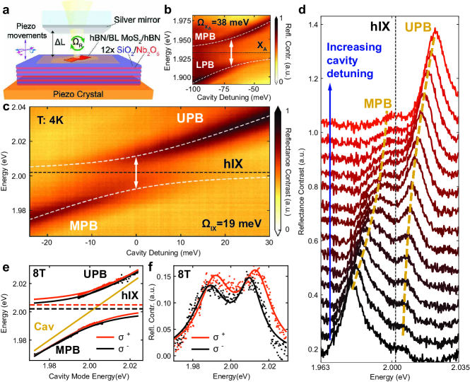
Figure 2: Strong exciton-photon coupling in MoS₂ bilayers. a, Schematics of the tunable open microcavity composed of a bottom DBR and a top semi-transparent silver mirror. b, c, Low temperature (4K) RC spectra measured as a function of the cavity-exciton detuning ($\Delta=E_{\mathrm{cav}}-E_{\mathrm{exc}}$) for cavity scans across b X_A and c hIX energies. White dotted lines show the fitting obtained using the coupled-oscillator model providing the Rabi splittings $\Omega_{\mathrm{hiX}}=19$ meV and $\Omega_{\mathrm{X_{A}}}=38$ meV. d, RC spectra measured for the cavity-exciton detunings in the vicinity of the anticrossing between hIX and the cavity mode. e, Dipolariton dispersion measured with circularly polarized detection for 8 T magnetic field. The orange and black solid curves are the coupled oscillator model fits for $\sigma^{+}$ and $\sigma^{-}$ detection, respectively. The positions of the Zeeman-split hIX peaks are shown by dashed lines. f, $\sigma^{+}$ (orange) and $\sigma^{-}$ (black) RC spectra measured at 8 T at the hIX-cavity anticrossing. Fitting with two Lorentzians (solid lines) is shown.

Our heterostructure samples consists of a MoS₂ bilayer (BL) sandwiched between hBN and placed on a distributed Bragg reflector (DBR). Fig. 1a shows a bright field microscope image of the encapsulated BL MoS₂. A sketch of the side view of the device is displayed in Fig. 1b. The reflectance contrast (RC) spectrum of the studied MoS₂ bilayer, displayed in Fig. 1c, shows three peaks: the intralayer neutral excitons X_A at at $1.937$ eV (see Fig. 1d), hybridized interlayer exciton hIX at $2.004$ eV and hybridized B-exciton at $2.113$ eV. Due to the quantum tunnelling of holes, B-excitons hybridize with an interlayer exciton (IX) (Fig. 1d), which is a direct transition in the bilayer momentum space [11]. The ratio of the integrated intensities of X_A and hIX is $4.5$. Based on these data, we estimate the electron-hole separation $d=0.55$ nm (see details in Supplementary Note S1) in agreement with previous studies [14]. We further confirm the nature of the hIX states by placing the BL MoS₂ in magnetic field where the valley degeneracy is lifted (Fig. 1e). In agreement with recent studies [13, 39], we measure a Zeeman splitting with an opposite sign and larger magnitude in hIX compared with X_A (-3.5 versus 1.5 meV).

We study the strong coupling regime in a tunable planar microcavity (Fig. 2a) formed by a silver mirror and a planar DBR [7]. RC scans as a function of the cavity mode detuning $\Delta=E_{cav}-E_{exc}$, where $E_{cav}$ and $E_{exc}$ are the cavity mode and the corresponding exciton energy, respectively, are shown in Fig. 2c,d. Characteristic anticrossings of the cavity mode with X_A and hIX are observed, resulting in lower, middle and upper polariton branches (LPB, MPB, and UPB, respectively). The extracted Rabi splittings are $\Omega_{\mathrm{X_{A}}}=38$ meV for X_A and $\Omega_{\mathrm{hIX}}=19$ meV for hIX (Supplementary Note S2). Fig. 2d shows the RC spectra in the vicinity of the anticrossing with hIX, providing a more detailed view of the formation of the MPB and UPB. The intensity of the polariton peaks is relatively low for the states with a high exciton fraction at positive (negative) cavity detunings for the MPB (UPB). As the Rabi splitting scales as a square root of the oscillator strength, the ratio $\Omega_{\mathrm{X_{A}}}/\Omega_{\mathrm{hIX}}=2$ is in a good agreement with the RC data for integrated intensities of X_A and hIX. From the Rabi splitting ratio we can estimate the tunneling constant $J$ leading to the exciton hybridization. The corresponding coefficient is $J=48$ meV (see Supplementary Note S1 for details), matching the density functional theory predictions [11]. In polarization-resolved cavity scans in an out-of-plane magnetic field (Fig. 2e,f), similarly to hIX behaviour, we observe opposite and larger Zeeman splitting for dipolaritons relative to the intralayer polaritons (see Supplementary Figure S4). Chiral dipolariton states are observed distinguished by their opposite circular polarization (Fig. 2f).

We investigate the nonlinear response of X_A and hIX in the bare BL flake as a function of the laser power using both narrow band (NB, full-width at half maximum, FWHM=28nm) and broad band (BB, FWHM=50 nm) pulsed excitation (see Methods). Our resonant pump-probe experiments have confirmed that the lifetimes of the hIX and X_A states are considerably longer than the pulse duration of $\approx 150$ fs (Supplementary Note S3). Measured RC spectra are shown in Fig. 3a,b for the NB and in Fig. 3c for BB excitation. In the NB case, the excitation was tuned to excite either X_A or hIX independently, while in the BB case, both resonances were excited simultaneously.

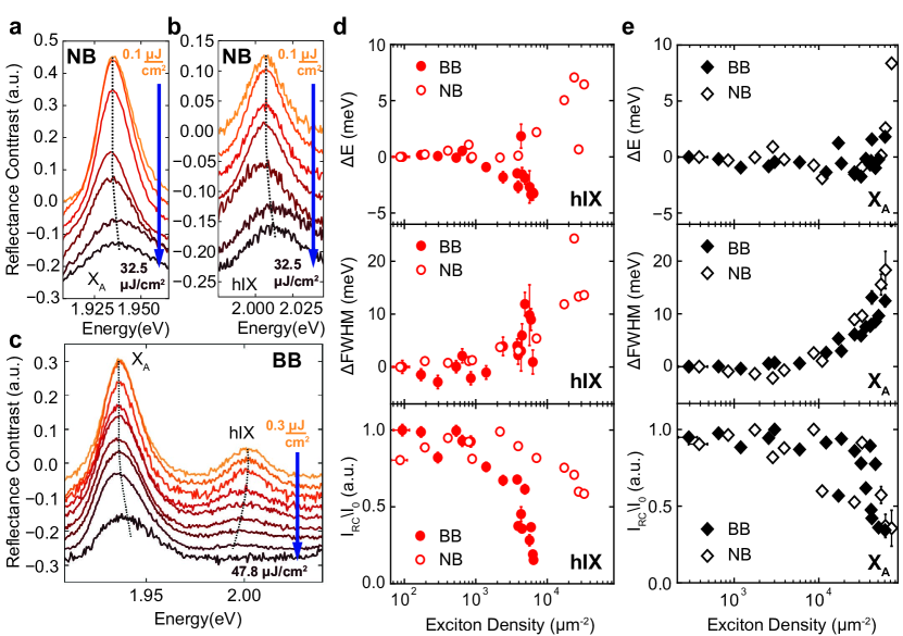
Figure 3: Exciton nonlinearity in MoS₂ bilayers. a, b, c, RC spectra measured with the NB (FWHM=28nm) excitation for the X_A (a) and hIX (b), and with the BB (FWHM=50nm) excitation (c) at different fluences. The dashed curves are guide for the eye. d, e, The energy shift $\Delta E$ (top), linewidth variation $\Delta$FWHM (middle) and normalized integrated intensity (bottom) as a function of the exciton density for the hIX (d) and X_A (e). Solid (open) symbols show the results for the BB (NB) excitation. For the normalized intensity we divide the intergrated intensity at each laser power by that at the maximum intensity.

As seen in Figs. 3a,b both X_A and hIX spectra behave similarly upon increasing the power of the NB excitation: a blueshift of several meV is observed, accompanied by the peak broadening and bleaching. For the BB excitation, however, a different nonlinear behaviour is observed as shown in Fig. 3c: the broadening and complete suppression of the hIX peak is observed at much lower powers, accompanied by a redshift. This is in contrast to X_A, whose behaviour is similar under the two excitation regimes.

The resulting energy shifts, peak linewidths and intensities are shown in Fig. 3d,e as a function of the exciton density (see details in Supplementary Note S4 and S6). Fig. 3d quantifies the trends observed in Figs. 3a,b showing for the BB excitation an abrupt bleaching of the hIX peak above the hIX density $5\times 10^{3}~{}\mu$m^-2 accompanied by a redshift of $\approx$ 4 meV and a 12 meV broadening. For the NB case, a similar decrease in peak intensity is observed only around $4\times 10^{4}~{}\mu$m^-2, accompanied with a peak blueshift of $\approx$ 7 meV and a broadening exceeding 15 meV. In Fig. 3e, however, it is apparent that the observed behaviour under the two excitation regimes is similar for X_A. A similar blueshift, broadening and saturation are observed at slightly higher densities compared to the hIX under the NB excitation (Supplementary Note S5). We also find that due to the increased excitonic Bohr radius, the onset of the nonlinear behaviour for X_A in bilayers occurs at a lower exciton density than for X_A in monolayers (Supplementary Note S7).

We develop a microscopic model to describe the contrasting phenomena under the NB and BB excitation. Under the NB excitation, either X_A or hIX excitons are created as sketched in Fig. 4a. In this case, nonlinearity arises from Coulomb exciton-exciton interactions causing the blueshift and dephasing [40]. For simplicity, in the main text we will use a Coulomb potential $V_{Coul}$ combining the exchange and direct terms further detailed in Supplementary Note S8. We confirm (see Supplementary Note S8) that for the intralayer exciton-exciton interaction (X_A-X_A) the dominant nonlinear contribution comes from the Coulomb exchange processes, as in the monolayer case [40, 41], while for the hIX-hIX scattering the dominant contribution is from the direct Coulomb (dipole-dipole) interaction terms [19]. For both X_A and hIX, the Coulomb interaction is repulsive, and thus leads to the experimentally observed blueshifts. We find that for the modest electron-hole separation $d=0.55$ nm in the bilayer, $V_{Coul}$ is overall 2.3 times stronger for hIX compared with X_A.

Analysing the shapes of the reflectance spectra in the NB case, we note that they depend on the rates of radiative ($\Gamma_{\mathrm{R}}$) and non-radiative ($\Gamma_{\mathrm{NR}}$) processes. The area under RC curves is described by the ratio $\Gamma_{\mathrm{R}}/(\Gamma_{\mathrm{R}}+\Gamma_{\mathrm{NR}})$. This ratio changes under the increased excitation if the rates depend on the exciton densities. Specifically, we account for the scattering-induced non-radiative processes that microscopically scale as $\Gamma_{\mathrm{NR}}\propto|V_{\mathrm{Coul}}|^{2}n$, i.e. depend on the absolute value of the combined matrix elements for the Coulomb interactions and the exciton density $n$ [40]. This process allows reproducing the RC behaviour and bleaching at increasing pump intensity. Moreover, it explains stronger nonlinearity for X_A in bilayers compared to monolayers. Namely, the scattering scales with the exciton Bohr radius, $V_{\mathrm{Coul}}\propto\alpha$, which is larger in the bilayers due to the enhanced screening (Supplementary Note S8).

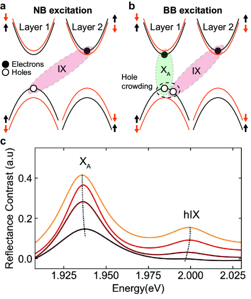
Figure 4: Theoretical model for nonlinear optical response in MoS₂ bilayers. a, b, Schematic diagram showing exciton generation under the NB (a) and BB (b) excitation. In (a) only generation of hIX is shown. In (b), the holes of the two excitonic species share the same valence band. c, Theoretically calculated absorption spectra for the BB excitation case (see Supplementary Note S8), providing qualitative agreement with the experiment. The dashed black curves are guides for the eye.

In the BB case, both X_A and hIX excitons are generated simultaneously, and together with intraspecies scattering (X_A-X_A and hIX-hIX), interspecies scattering (X_A-hIX) occurs, similarly to the direct-indirect exciton Coulomb scattering in double quantum wells [42]. Since X_A and hIX are formed by the holes from the same valence band (Fig. 4a), an additional contribution arises from the phase space filling, i.e. the commutation relations for the excitons (composite bosons) start to deviate from the ideal weak-density limit once more particles are created [43]. For particles of the same flavour, the phase space filling enables nonlinear saturation effects in the strong coupling regime, similar to polariton saturation observed in [29]. However, in the presence of several exciton species, we reveal a distinct phase space filling mechanism which we term the hole crowding. Crucially, we observe that the commutator of the X_A annihilation operator ($\hat{X}$) and hIX creation operator ($\hat{I}^{\dagger}$) is non-zero, $[\hat{X}(\mathbf{p}),\hat{I}^{\dagger}(\mathbf{q})]=-\hat{B}_{\mathbf{p},\mathbf{q}}$. Here $\mathbf{p}$, $\mathbf{q}$ are exciton momenta and $\hat{B}_{\mathbf{p},\mathbf{q}}$ is an operator denoting the deviation from the ideal commuting case ($\hat{B}_{\mathbf{p},\mathbf{q}}=0$) of distinct bosons where holes do not compete for the valence band space.

This statistical property of modes that share a hole has profound consequences for the nonlinear response. Namely, the total energy is evaluated as an expectation value over a many-body state with both X_A and hIX excitons, $|N_{\mathrm{X}},N_{\mathrm{hIX}}\rangle:=(\prod_{\mathbf{p}}^{N_{\mathrm{X}}}\hat{X}^{\dagger})(\prod_{\mathbf{q}}^{N_{\mathrm{hIX}}}\hat{I}^{\dagger})|\Omega_{max}\rangle$, where $N_{\mathrm{X}}$ and $N_{\mathrm{hIX}}$ particles are created from the ground state $|\Omega_{max}\rangle$. If the excitonic modes are independent, the contributions from X_A and hIX simply add up. However, the hole coexistence in the valence band induces the excitonic interspecies scattering. The phase space filling combined with the Coulomb energy correction leads to a negative nonlinear energy contribution. This nonlinear term scales as $\Delta E_{\mathrm{hIX}}=-\eta\sqrt{n_{\mathrm{X}}n_{\mathrm{hIX}}}$, where $\eta>0$ is a coefficient defined by the Coulomb energy and Bohr radii and $n_{\mathrm{X,hIX}}$ are the exciton densities (see Supplementary Note S9). This nonlinearity also modifies the non-radiative processes leading to substantial broadening for the hIX states.

According to this analysis, the effect of the BB excitation should be most pronounced for hIX. In addition to the possible hIX-hIX scattering (similar to that occurring under the NB excitation), much stronger X_A absorption leads to the phase space filling in the valence band. Such hole crowding introduces additional scattering channels for hIX and leads to its RC spectra bleaching at lower hIX exciton densities. On the other hand, as only relatively small hIX densities can be generated, both the NB and BB excitation cases should produce similar results for X_A. Using the estimated nonlinear coefficients caused by the hole crowding, we model the RC in the BB regime and qualitatively reproduce the strong bleaching and redshift for hIX at the increased density.

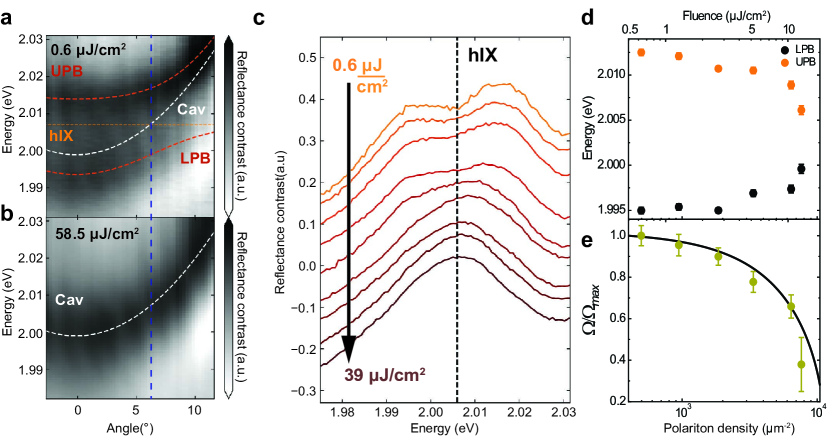
Figure 5: Nonlinear behaviour of dipolaritons. a, b, Reflectance contrast spectra measured at different laser fluences for the MoS₂ bilayer placed in a monolithic cavity. (a) The low fluence case (0.6 $\mu$J cm^-2). A clear anticrossing at 6.5°is observed. Dashed red lines show the results of the fitting using a coupled oscillator model, with two polariton branches LPB and UPB formed. White and orange lines show the energies of the uncoupled cavity mode and hIX state, respectively. The vertical line marks the anticrossing angle. (b) The high fluence case (58.5 $\mu$J cm^-2). A complete collapse of the strong coupling regime is observed, with the disappearance of the anticrossing and transition into the weak coupling regime. c, RC spectra measured at the anticrossing at 6.5° as a function of the laser fluence. d, Measured UPB and LPB peak energies at 6.5° as a function of the laser fluence (see top axis) and the corresponding polariton density (bottom axis). e, Symbols show the Rabi splittings normalized by the Rabi splitting measured at the lowest power ($\Omega$/$\Omega_{max}$) as deduced from d,. The line shows the fitting using our theoretical model (Supplementary Note S8).

We investigate nonlinear properties of dipolar polaritons in a monolithic (fixed-length) cavity created by a silver mirror on top of a PMMA spacer (245 nm thick) covering the hBN-encapsulated MoS₂ homobilayer placed on the DBR. The cavity mode energy can be tuned by varying the angle of observation (0 degrees corresponds to normal incidence). We use a microscopy setup optimized for Fourier-plane imaging, thus allowing simultaneous detection of reflectivity spectra in a range of angles as shown in Fig.5(a) displaying the measured polariton dispersion. In this experiment, the cavity mode is tuned around hIX and only two polariton branches LPB and UPB are observed at low fluence of 0.6 $\mu$J cm^-2 with a characteristic Rabi splitting of 17.5 meV. In Fig.5(b), at an increased fluence of 58.5 $\mu$J cm^-2, only a weakly coupled cavity mode is visible.

Fig.5(c) shows RC spectra taken at $\sim 6.5$° around the anticrossing at different laser fluences. The collapse of the two polariton peaks into one peak signifying the transition to the weak coupling regime is observed above 25 $\mu$J cm^-2. The LPB and UPB energies extracted using the coupled oscillator model (Supplementary Figure S5) are shown in Fig.5(d). As the polariton density is increased, the LPB and UPB approach each other almost symmetrically, converging to the exciton energy. The corresponding normalized Rabi splitting ($\Omega/\Omega_{max}$, where $\Omega_{max}$ is measured at low fluence) are shown in Fig.5(d,e) as a function of the total polariton density.

In this experiment, the cavity mode is considerably above the X_A energy, which therefore is not coupled to the cavity. Hence, the extracted Rabi splittings are fitted with a theoretically predicted trend of $\Omega$ for the NB excitation regime (Supplementary Note S8). A nonlinear polariton coefficient $\beta=0.86~{}\mu$eV$\mu$m² is extracted by differentiating the fitted function with respect to the polariton density. Comparing our results to X_A intralayer-exciton-polaritons in monolayers in similar cavities [16], we observe that the nonlinearity coefficient for dipolar interlayer polaritons is about an order of magnitude larger. This is in a good agreement with the theoretically predicted intrinsic nonlinearity of hybridized interlayer polaritons (Supplementary Note S8), and with our experimental data comparing hIX and monolayer X_A outside the cavity (Supplementary Note S7).

In summary, we report the nonlinear exciton and exciton-polariton behaviour in MoS₂ homobilayers, a unique system where hybridized interlayer exciton states can be realized having a large oscillator strength. We find that nonlinearity in MoS₂ bilayers can be enhanced when both the intralayer and interlayer states are excited simultaneously, the regime that qualitatively changes the exciton-exciton interaction through the hole crowiding effect introduced theoretically in our work. In this broad-band excitation regime, the bleaching of the hIX absorption occurs at 8 times lower hIX densities compared to the case when the interlayer excitons are generated on their own. In addition to this, we find that the dipolar nature of hIX states in MoS₂ homobilayers already results in 10 times stronger nonlinearity compared with the intralayer excitons in MoS₂ monolayers. Thus, we report on an overall enhancement of the nonlinearity by nearly two orders of magnitude. Thanks to the large oscillator strength, hIX can enter the strong coupling regime in MoS₂ bilayers placed in microcavities, as realized in our work. Similarly to hIX states themselves, dipolar polaritons also show 10 times stronger nonlinearity compared with exciton-polaritons in MoS₂ monolayers. We expect that in microcavities where the cavity mode is coupled to both hIX and X_A in MoS₂ bilayers, and the excitation similar to the broad-band regime can thus be realized, the nonlinear polariton coefficient will be dramatically enhanced owing to the hole crowding effect, allowing highly nonlinear polariton system to be realized. We thus predict that MoS₂ bilayers will be an attractive platform for realization of quantum-correlated polaritons with applications in polariton logic networks [20] and polariton blockade [21, 22].

I Methods

The hBN/MoS₂/hBN heterostructures were assembled using a PDMS polymer stamp method. The PMMA spacer for the monolithic cavity was deposited using a spin-coating technique, while a silver mirror of 45 nm was thermally evaporated on top of it.

Broad-band excitation was used to measure the reflectance contrast (RC) spectra of the devices at cryogenic temperatures (4K), defined as $\mathrm{RC}=(R_{\mathrm{sub}}-R_{\mathrm{BL}})/R_{\mathrm{sub}}$, where $R_{\mathrm{sub}}$ and $R_{\mathrm{BL}}$ are the substrate and MoS₂ bilayer reflectivity, respectively. For the magnetic field studies the same RC measurements were performed using unpolarized light in excitation with polarizers, $\lambda/4$ polarizers and $\lambda/2$ waveplates in collection, to resolve $\sigma^{+}$ and $\sigma^{-}$ polarization. The low temperature measurements using the tunable cavity were carried out in a liquid helium bath cryostat (T=4.2K) equipped with a superconducting magnet and free beam optical access. We used a white light LED as a source. RC spectra were measured at each $\Delta L$ and are integrated over the angles within 5 degrees from normal incidence. The RC spectra measured in the cavity are fitted using Lorenzians. The peak positions are then used to fit to a coupled oscillator model, producing the Rabi splitting and the exciton and cavity mode energies.

The measurements on the monolithic cavity were performed in a closed loop helium flow cryostat (T=6K). For the power-dependent RC experiments, we used supercontinuum radiation produced by 100 fs Ti:Sapphire laser pulses at 2 kHz repetition rate at 1.55 eV propagating through a thin sapphire crystal. The supercontinuun radiation was then filtered to produce the desired narrow-band excitation.

All the exciton and polariton densities were calculated following the procedure introduced by L. Zhang et al. [16], taking into account the spectral overlap of the spectrum of the excitation laser and the investigated exciton peak (see further details in Supplementary Note S4).

II Acknowledgements

CL, AG, TPL, SR and AIT acknowledge financial support of the European Graphene Flagship Project under grant agreement 881603 and EPSRC grants EP/V006975/1, EP/V026496/1, EP/V034804/1 and EP/S030751/1. TPL acknowledges financial support from the EPSRC Doctoral Prize Fellowship scheme. CT, SDC and GC acknowledge support by the European Union Horizon 2020 Programme under Grant Agreement 881603 Graphene Core 3. AG and GC acknowledge support by the European Union Marie Sklodowska-Curie Actions project ENOSIS H2020-MSCA-IF-2020-101029644. PC, RJ and DGL thank EPSRC Programme Grant ‘Hybrid Polaritonics’ (EP/M025330/1).

III Author contributions

CL and SR fabricated and characterized hBN-encapsulated MoS₂ samples. KW and TT synthesized the high quality hBN. CL and AG designed the microcavity samples. PC, RJ, DGL fabricated the microcavity samples. CL, AG, CT, TL and SDC carried out optical spectroscopy experiments. SC and OK developed theory. AG calculated polariton densities. CL and AG analyzed the data with contribution from AIT, TL, SC, OK, CT, SDC and GC. CL, AG, SC, OK and AIT wrote the manuscript with contribution from all other co-authors. AIT, OK, DGL, GC managed various aspects of the project. AIT supervised the project.

Supplementary Information: Nonlinear Interactions of Dipolar Excitons and Polaritons in MoS₂ Bilayers

Charalambos Louca,^1,⋆ Armando Genco,^2,† Salvatore Chiavazzo,³ Thomas P. Lyons,^1,4 Sam Randerson,¹ Chiara Trovatello,² Peter Claronino,¹ Rahul Jayaprakash,¹ Kenji Watanabe,⁵ Takashi Taniguchi,⁵ Stefano Dal Conte,² David G. Lidzey,¹ Giulio Cerullo,² Oleksandr Kyriienko,³ and Alexander I. Tartakovskii^1,‡

¹Department of Physics and Astronomy, The University of Sheffield, Sheffield S3 7RH, UK
²Dipartimento di Fisica, Politecnico di Milano, Piazza Leonardo da Vinci, 32, Milano, 20133, Italy
³Department of Physics, University of Exeter, Stocker Road, Exeter, EX4 4PY, UK
⁴RIKEN Center for Emergent Matter Science, Wako, Saitama, 351-0198, Japan
⁵Advanced Materials Laboratory, National Institute for Materials Science, 1-1 Namiki, Tsukuba, 305-0044, Japan

Supplementary Note S4: Supplementary Note S1: Theoretical estimate of exciton properties — energy and hybridisation

In this section of Supplemental Materials we describe details of theoretical description of MoS₂ homobilayers. Properties of excitons in a bilayer system have been discussed in the main text, and we support them by modelling. The optical response of the system is characterised by the response of three different species of quasi-particles, namely X_A, hIX and hX_B (see main text). Here we provide an intuitive picture of the homobilayer physics and estimate the system parameters. In particular, we estimate exciton Bohr radii and a hole tunnelling rate as relevant parameters when studying nonlinear properties.

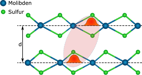
Supplementary Figure S1: Side view of 2H-stacked MoS₂ bilayer. Blue spheres are Mo (molybdenum) atoms and green are S (sulphide) atoms. We picture a hole wave function in each layer, constructing a hybrid state through tunneling process (hole delocalisation). This allows for hybrid hX_B and hIX excitons. We define the distance between the layer as the distance between particle centres of charge. In absence of external fields, the centre of charge is located in between the S planes [44].

We consider a MoS₂ homobilayer system with 2H stacking (see Fig. S1). This is comprised of two parallel layers of MoS₂, with centres located at a distance $d$ from each other (charge separation distance). The physics of bilayers is defined by properties of electrons and holes that interact through the Keldysh-Rytova potential [45, 46, 47], being different for in-plane and out-of-plane interaction [48]. Within the $k\cdot p$ framework, electrons and holes are treated as particles with effective mass provided by a band dispersion. In MoS₂ the typical values for effective masses are $0.46$ m_e for conduction bands and $0.56$ m_e for the valence bands (with m_e being the electron mass) [11, 49]. The attractive Kledysh-Rytova potential has a different form depending on the relative position between particles. We call $V^{\mathrm{intra}}_{\mathrm{KR}}$ the attractive potential of particles being in the same layer, and $V^{\mathrm{inter}}_{\mathrm{KR}}$ the attractive potential of particles being in separate layers. In momentum space the different potentials read as

$$V^{\mathrm{intra}}_{\mathrm{KR}}(\mathbf{q})= -\frac{e^{2}}{4\pi\epsilon\epsilon_{\mathrm{0}}}\frac{1+(r_{\mathrm{0}}q/\epsilon)(1-\exp(-2qd))}{(1+r_{\mathrm{0}}q/\epsilon)^{2}-(r_{\mathrm{0}}q/\epsilon)^{2}\exp(-2qd)},$$ (S1a)

$$V^{\mathrm{inter}}_{\mathrm{KR}}(\mathbf{q})= -\frac{e^{2}}{4\pi\epsilon\epsilon_{\mathrm{0}}}\frac{\exp(-qd)}{(1+r_{\mathrm{0}}q/\epsilon)^{2}-(r_{\mathrm{0}}q/\epsilon)^{2}\exp(-2qd)},$$ (S1b)

where $e$ is the electron charge, $\epsilon_{\mathrm{0}}$ is the vacuum permittivity, $\epsilon$ in an average environment permittivity, $r_{\mathrm{0}}$ is a screening length (defined as for monolayers), and $\mathbf{q}$ is an exchanged particle momentum [48]. We compute a binding energy of an exciton bound state by assuming the Keldysh-Rytova attractive potential and free particle dispersion defined by the effective masses. To provide a simple understanding of the system, we approach the problem using an ansatz wavefunction $\phi(\rho)=\sqrt{2/\pi\alpha^{2}}\exp(-\rho/\alpha)$, with $\rho$ being the in-plane projection of electron-hole distance and $\alpha$ the exciton Bohr radius. This describes well an internal structure of an exciton, and gives the information about its shape, collected in the Bohr radius. In Fourier space, the function $\phi(q)$ reads

$$\phi(q)=\sqrt{\frac{2}{\pi}}\frac{\alpha}{(1+q^{2}\alpha^{2})^{3/2}}.$$ (S2)

With the given wave function [Eq. (S2)], and the given potentials [Eq. (S1)], we can find the binding energy and the Bohr radius of the excitons by minimizing the energy of the system. This procedure is performed in the range of possible interlayer separation $d$. Fig. S2(a) shows the energy change with the separation. The blue curve corresponds to the hIX mode, while orange and red curves correspond to X_A and hX_B, respectively. We considered a band-gap of $2.12$ eV, and spin-orbit splitting of $13$ meV for conduction band and $150$ meV for valence band, as suggested by the ab initial calculations [49].

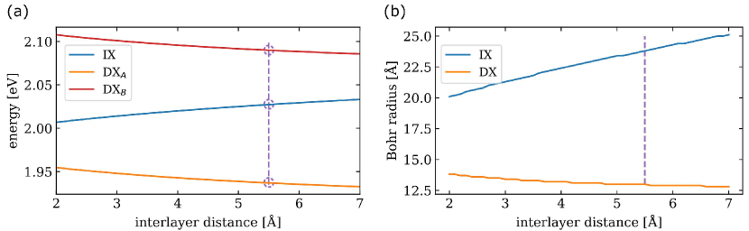
Supplementary Figure S2: Evolution of particle properties with interlayer distance. a) Energy of quasiparticle modes with distance. The blue line is the hIX mode, and the orange and red respectively are X_A and hX_B. The redshift of direct modes with the increase of interlayer distance is due to reduced screening effects, as characteristic of Keldysh-Rytova potential in Eq. (S1). On the contrary, the hIX mode sees a blueshift that is due to the lower attraction of particles located in separate layers. The purple dashed line is the distance to match with the experimental data. b) Dependence of Bohr radius with interlayer distance. Here we only report one direct exciton as both A and B excitons have the same behavior. The orange one is the evolution for direct excitons, and the blue line is for indirect excitons. Both plots (a) and (b) show similiar increase (or increase) with distance as the screening mechanism affects the considered parameters the same way. This analysis reveals the hIX Bohr radius to be roughly twice as much as the X one.

Here we estimate the interlayer distance $d$ thanks to experimental knowledge of energy distance between exciton energy modes. Note the peak of X_A mode is not shifted by any tunneling, while X_B and IX are coupled through tunneling constant $J$ [50]. That is, the theoretical energy distance $\Delta_{\mathrm{0}}$ between the two modes has to be fixed to match the experimental result $\Delta=109$ meV. With considering two coupled harmonic oscillators, we find the corrected energy shift to be

$$\Delta=\sqrt{\Delta_{\mathrm{0}}^{2}+4J^{2}}.$$ (S3)

By matching with the experimental data for the energy distance between modes, we extract $d=5.5$ Å and estimate the effective tunneling rate to be $J=45$ meV. As a consequence, $21\%$ of X_B oscillator strength is transferred to IX mode, in agreement with previous observations [11]. Finally, Fig. S2(b) shows the evolution of particle Bohr radii with the interlayer distance. We respectively call the Bohr radius of direct and indirect exciton $\alpha_{\mathrm{D}}$ and $\alpha_{\mathrm{I}}$. The blue curve is the Bohr radius of hIX, while the orange one described the X modes. With X_A and hX_B being very similar, we describe both with one orange curve. The energy separation is provided only by the spin-orbit splitting. Typical values of $\alpha_{\mathrm{D}}$ are approximately $1$ nm, with $\alpha_{\mathrm{I}}$ being approximately $2$ nm. Note the opposite behavior of $\alpha_{\mathrm{D}}$ and $\alpha_{\mathrm{I}}$ with distance. hIX Bohr radius grows with distance due to the reduced attraction between particles in separate layers. On the contrary, by increasing the interlayer distance, we see the reduced screening for particles in the same layer, resulting in a decrease of the Bohr radius and consequent increase of the binding energy.

Supplementary Note S5: Supplementary Note S2: Coupled oscillator model

A full picture of our system, corresponding to MoS₂ homobilayer, has to take into account 4 different modes coupling to each other: only IX and X_B hybridise through a tunneling parameter, while X_A and X_B can couple with the cavity due to their high oscillator strength. We can then simplify this picture by rewriting the IX and X_B states in terms of the new basis of hybridised modes, hIX and hX_B, as defined in the main text, all of them now capable of a coupling with the cavity mode. The corresponding Hamiltonian reads

$$H=\left(\begin{array}[]{cccc}{E}_{\mathrm{c}}&\Omega_{\mathrm{X_{A}}}&\Omega_{\mathrm{hIX}}&\Omega_{\mathrm{hX_{B}}}\\ \Omega_{\mathrm{X_{A}}}&E_{\mathrm{X_{A}}}&0&0\\ \Omega_{\mathrm{hIX}}&0&E_{\mathrm{hIX}}&0\\ \Omega_{\mathrm{hX_{B}}}&0&0&E_{\mathrm{hX_{B}}}\end{array}\right),$$ (S4)

where $E_{\mathrm{c}}$ in the energy of the cavity mode, and $E_{\mathrm{X_{A}}}$, $E_{\mathrm{hIX}}$, $E_{\mathrm{hX_{B}}}$ denote energies of the respective excitonic modes. Here, $\Omega_{\mathrm{X_{A}}}$, $\Omega_{\mathrm{hIX}}$, and $\Omega_{\mathrm{hX_{B}}}$ are corresponding matrix elements for light-matter coupling (Rabi splittings).

Due to the large energy separation between the resonances, each splitting can be fitted to a two level oscillator model independently. In our case, the spectra from the open cavity scans at piezo voltages close to resonant anticrossings between the cavity and either X_A or hIX, were fitted with Lorenzian functions. The results were then fitted to the respective Hamiltonians of two coupled oscillators, such that $H_{\mathrm{A}}=\left(\begin{array}[]{cc}{E}_{\mathrm{c}}&\Omega_{\mathrm{X_{A}}}\\ \Omega_{\mathrm{X_{A}}}&E_{\mathrm{X_{A}}}\end{array}\right)$ and $H_{\mathrm{h_{IX}}}=\left(\begin{array}[]{cc}{E}_{\mathrm{c}}&\Omega_{\mathrm{hIX}}\\ \Omega_{\mathrm{hIX}}&E_{\mathrm{hIX}}\end{array}\right)$ and the values of Rabi splittings and resonant energies were extracted. The results of the fit are shown in Fig. S3

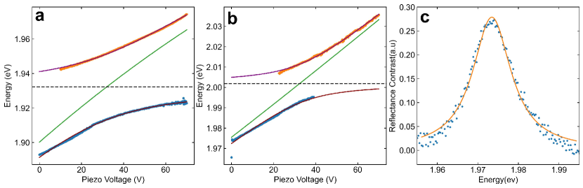
Supplementary Figure S3: Coupled oscillator model fits. a), b) Orange and blue dots represent the extracted peak energies of individual spectra near the a) X_A and b) hIX energies. The solid purple (UPB) and red (LPB) curves are the solutions to the fitted coupled oscillator Hamiltonians, and the green solid line is the extracted cavity mode energy as a function of voltage. c) shows a spectrum of the uncoupled cavity mode. A Lorenzian peak (orange) is fitted to the data (blue dots) and the linewidth is extracted to be equal to 11 meV, confirming that the condition for strong coupling regime is met, $\Omega^{2}>({\gamma_{c}}^{2}+{\gamma_{x}}^{2})/2$ as stated by [51].

In the presence of an out of plane magnetic field of 8 T, the same scans were repeated with unpolarised excitation and detecting opposite circularly polarized light $\sigma^{+}$/$\sigma^{-}$ at each piezo voltage. Fig. S4 shows the coupled oscillator fits with data from $\sigma^{+}$ and $\sigma^{-}$ detection of the X_A scan. It can be seen that the X_A-polaritons exhibit an opposite sign of Zeeman splitting compared to hIX-polaritons (shown in the main text).

Coupled oscillator models were also used for our monolithic cavity sample whose angular dispersion was measured with Fourier space imaging, as mentioned in the main text. The colour map with the extracted data points is presented in Fig. S5, with the overlaid couple oscillator fits.

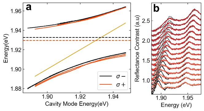
Supplementary Figure S4: Zeeman Splitting of X_A-polaritons. a) Tunable cavity RC scans near X_A energies. Orange and black colours represent $\sigma^{+}$ and $\sigma^{-}$ detection respectively. Dots represent the extracted peak energies of individual spectra. The solid orange and black curves are the solutions to the fitted coupled oscillator Hamiltonians and the golden solid line is the extracted cavity mode energy. The extracted exciton energies are shown in the plot as the dashed horizontal lines of the corresponding colour. It can be seen that the Zeeman splitting of X_A polaritons is of opposite sign to that of the hIX. The deviation of the $\sigma^{+}$ LPB datapoints from the coupled oscillator model solution (solid line) is due to the presence of the fully polarised trion at $\approx$ 1.91 eV. This can be seen as a broadening due to weak coupling of the lower energy peak of the orange ($\sigma^{+}$) spectra in b), where a cascade plot of the spectra near resonance in the two polarizations is shown.

Supplementary Figure S5: Coupled oscillator model fits on monolithic cavity. Monolithic cavity dispersion near hIX with couple oscillator model fits. Blue and green points show the extracted peak positions of the LPB and UPB, respectively, from the spectra at each angle. These are then fitted to the two level coupled oscillator model and the solutions LPB and UPB are shown as dark orange dashed curves. The extracted cavity mode and exciton energy are shown as white and light orange dashed curves, respectively.

Supplementary Note S6: Supplementary Note S3: Pump-probe resonant spectroscopy

We performed time-resolved resonant pump-probe spectroscopy on the encapsulated BL MoS₂ out of the cavity, to measure the X_A and hIX lifetimes in our system. Due to the small size of the samples, a microscopy setup allowing transient reflection measurements at low temperatures has been employed (Fig. S6 (a)). The setup is powered by an amplified Ti:sapphire laser (Coherent Libra) generating 100 fs pulses at 800 nm (1.55 eV) with 2 mJ pulse energy and 2 kHz repetition rate. A fraction of the laser output is used to seed a non-collinear optical parametric amplifier (NOPA) in the visible energy range. The generated pump pulses are modulated by a mechanical chopper at 500 Hz frequency. The broad-band probe pulses consist of a white-light continuum (WLC), generated from a 1-mm thick sapphire plate pumped by focusing the 800 nm output of the main laser. Pump and probe pulses are synchronized by means of a motorized delay stage. Pump and probe beams are then collinearly combined by a thin dichroic beam splitter and focused on the sample using an objective lens (NA=0.3), resulting in a 4$\mu m$ spot size. The samples are placed in a closed-cycle helium cryostat reaching a temperature of 6 K. The spatial overlap of the sample with the pump and probe spots is obtained by a three-axis (xyz) mechanical translation stage coupled to a home-built imaging system. After the interaction with the excited sample, the reflected probe pulse is collimated by the same objective lens and then sent to a spectrometer equipped with an electronically cooled Si CCD, to measure the differential reflection ($\Delta R/R$) signal.

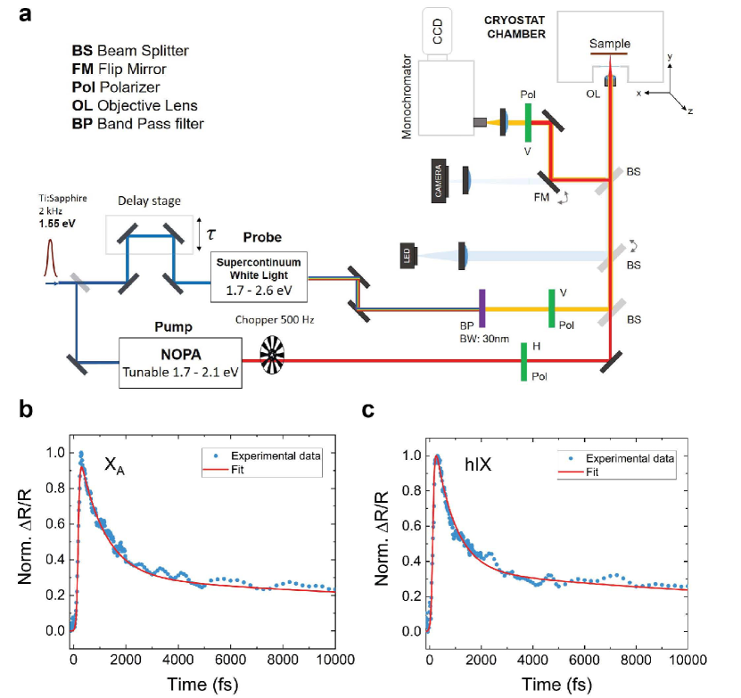
Supplementary Figure S6: a) Schematics of the pump-probe microscopy setup used for the experiments on the MoS₂ bilayers. b, c) Transient reflectivity traces for X_A (b) and hIX (c) taken at 643 nm and 622 nm respectively. The red curves refer to the fitted bi-exponential decay function.

Figure S6 (b,c) shows the temporal exciton dynamics measured as the absorption bleaching signal in transient reflectivity, taken at the peak wavelengths of the pump-probe traces, 643 nm and 622 nm for X_A and hIX respectively. For this experiment narrow-band pump pulses (FWHM=10nm) are tuned in resonance with each probed exciton and cross-polarized with respect to the probe pulses. The pump beam is then filtered by an additional polariser placed in the detection path before reaching the CCD. The probe spectral window has a narrow bandwidth of 30 nm with a central wavelength fixed at each exciton peak wavelength. The excitons decay traces show a fast component more prominent than the slow one, and can be fitted with a bi-exponential function convoluted with a Gaussian, taking into account the instrument response function. The resulting decay times are $\tau\textsubscript{fast}\approx 950$ fs, $\tau\textsubscript{slow}\approx 20$ ps for X_A, and $\tau\textsubscript{fast}\approx 780$ fs, $\tau\textsubscript{slow}\approx 18$ ps for hIX. Considering the degeneracy of pump and probe energies in our experiments, the fast decay can be attributed to electron-phonon scattering processes from the K point to the lowest energy Q point of the Brillouin zone [52, 53], while the slow component is possibly related to radiative [54] or defect-mediated non-radiative recombination [55]. We conclude that in our MoS₂ bilayer sample the fast and slow decay times for both X_A and hIX are much longer than the temporal width of the probe pulses ($\approx 150$ fs).

Supplementary Note S7: Supplementary Note S4: Density estimation

Exciton and polariton densities were calculated using an experimental approach considering a convolution of the laser profile and the Reflectance Contrast spectra, as in [16]. Reflectance contrast, A_res, represents with good approximation the absorption of the each excitonic/polaritonic resonance [16]. Power absorbed by each exciton/polariton, ${P}_{{\rm{res}}}$, can be calculated as

$${P}_{{\rm{res}}}=\frac{P\int L(E){{\rm{A}}}_{{\rm{res}}}(E){\rm{d}}E}{{I}_{{\rm{l}}{\rm{a}}{\rm{s}}{\rm{e}}{\rm{r}}}},$$ (S5)

where $P$ is the experimentally measured power, $\int L(E){{\rm{A}}}_{{\rm{res}}}(E){\rm{d}}E$ is the convolution of the laser spectrum profile, L(E), and the Reflectance Contrast spectrum in the range of energies of the resonant transition peak and $I_{\rm{laser}}=\int L(E){\rm{d}}E$ is the laser spectrum integrated intensity.

The expression (S5) can then be used to calculate the particle density, $n_{\rm{res}}$, considering the laser repetition rate, $R_{\rm{laser}}$, laser spot size, $S_{\rm{laser}}$, and the excitation central energy, $E_{\rm{res}}$. Explicitly, an estimate for the density reads

$$n_{\rm{res}}=\frac{{P}_{{\rm{res}}}}{R_{\rm{laser}}E_{\rm{res}}S_{\rm{laser}}}.$$ (S6)

We note that for the polariton density estimations, since A_res is dependent on the angle, ${P}_{{\rm{res}}}$ was calculated integrating all the spectral quantities in both the energy and angular range of LPB and UPB. As such, the densities calculated with this procedure are the total polariton densities, which consider both LPB and UPB.

For the values of polariton/exciton densities the error, $\rm{\epsilon_{n}}=\sqrt{{\left(\frac{{\rm{\epsilon}}_{{P}_{\rm{res}}}}{{P}_{{\rm{res}}}}\right)}^{2}+{\left(\frac{{\rm{\epsilon}}_{{E}_{{\rm{res}}}}}{{E}_{{\rm{res}}}}\right)}^{2}}$, is propagated with respect to standard error analysis rules [56]

Supplementary Note S8: Supplementary Note S5: Comparison of hIX and X_A nonlinearity under NB illumination

As mentioned in the text, the nonlinear behaviour of hIX is a slightly enhanced compared to X_A. The Supplementary Figure S7 shows the data of Fig. 3 in the main text such that a direct comparison between the two exciton species under separate narrow band (NB) illumination can be evaluated.

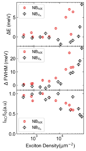
Supplementary Figure S7: From top to bottom: plots of the energy shift ($\Delta E$), linewidth variation ($\Delta$FWHM) and normalised integrated intensity ($I_{\mathrm{RC}}/I_{0}$, where$I_{0}$ is the maximum integrated intensity) as a function density for hIX (red marks in Fig. 3d) and X_A (black marks in Fig. 3e) peaks measured in RC. hIX is bleaching, broadening and blueshifting at slightly lower densities compared to X_A

Supplementary Note S9: Supplementary Note S6: hIX and X_A spectral fluence dependencies

Data shown in Fig. 3 of the main text are presented here in Supplementary Figure S8 as a function of the raw spectral fluence. We define spectral fluence as the experimentally measured fluence normalised by the illumination spectral width in electron volts.

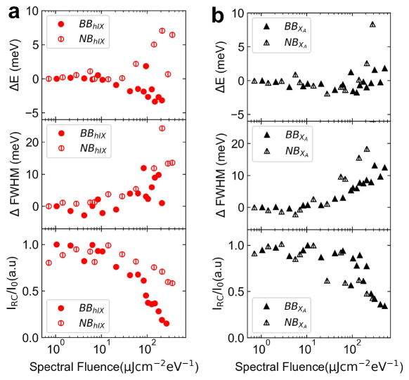
Supplementary Figure S8: MoS₂ bilayer excitons nonlinear behaviour against spectral fluence a), b) From top to bottom: plots of the energy shift ($\Delta E$), linewidth variation ($\Delta$FWHM) and normalised integrated intensity ($I_{\mathrm{RC}}/I_{0}$, where $I_{0}$ is the maximum integrated intensity) as a function of the incident fluence normalised by the spectral width (Spectral Fluence) for hIX (red marks in d) and X_A (black marks in e) peaks measured in RC. Solid marks relate to the experiments with BB excitation, covering both the hIX and the X_A, while open marks refer to the NB excitation, at either the hIX or the X_A energy.

Supplementary Note S10: Supplementary Note S7: Monolayer MoS₂ excitons nonlinear behaviour

The density dependent nonlinearity was studied for an encapsulated MoS₂ monolayer on an identical DBR substrate outside the cavity, in narrow band (NB) illumination regime ($\approx$20 nm bandwidth). The results are then compared against the bilayer excitons excited with NB illumination. A less significant bleaching of excitons in the monolayer is clearly apparent, confirming the theoretical predictions of increased interactions in bilayer excitons. Extrapolation such data, we estimate that the monolayer to reach complete bleaching at up to an order of magnitude higher densities.

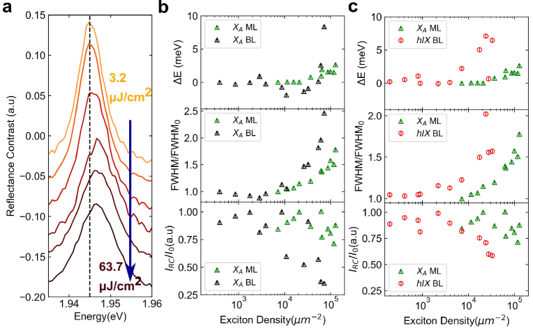
Supplementary Figure S9: MoS₂ monolayer excitons nonlinear behaviour. a) Waterfall of monolayer X_A RC spectra with the darker colours representing larger pump powers. Despite a blueshift is apparent,, the exciton bleaching is much less pronounced than for the bilayer excitons. b, c) Nonlinearity comparison of monolayer X_A to bilayer X_A (b) and hIX (c). From top to bottom: plots of the energy shift ($\Delta E$), normalised ($FWHM/FWHM_{0}$) and normalised integrated intensity ($I_{\mathrm{RC}}/I_{0}$, where$I_{0}$ is the maximum integrated intensity) as a function of exciton density, for the monolayer X_A (green), bilayer X_A(black) and hIX (red) under narrow band excitation.

Supplementary Note S11: Supplementary Note S8: Theoretical discussion on interaction constants

In our work we observed several nonlinear effects with contributions that depend on excitation conditions. In the BB regime, we already discussed the presence of two main species (flavours) of particles, namely direct X and indirect hIX excitons, determining the features of the sample’s optical response. This can be seen from the reflectance spectra in Fig. 2(a) and (b) of main text. We observe both the energy shifts (discussed above), and additional bleaching of the peaks. This hints that the presence of conservative nonlinear processes (energy shifts) is accompanied by dissipative nonlinear processes. Below, we discuss various contributions, including the Coulomb-mediated scattering, optical saturation due to phase space filling, and nonlinear change of non-radiative decay and dephasing processes.

We stress that in general all the aforementioned processes contribute to the spectral signal we observed. The peak shape is due to the competing contribution of radiative and non-radiative decay processes. Both radiative $\Gamma_{\mathrm{R}}$ and non-radiative $\Gamma_{\mathrm{NR}}$ rates depend on the particle densities $n_{\mathrm{D}}$ and $n_{\mathrm{I}}$, for direct and interlayer excitons respectively. Here we simply refer to some generic density $n$, without specifying the particle flavour involved, as similar consideration apply to both. We relate the exciton radiative decay rate and the Rabi frequency $\Omega$ for polaritons, as they are both proportional to the particle oscillator strength $\Gamma_{\mathrm{R}},\Omega\propto f_{\mathrm{osc}}$ [1]. More accurately, we know that $\Gamma_{\mathrm{R}}\propto f_{\mathrm{osc}}$, and $\Omega(n)\propto\sqrt{f_{\mathrm{osc}}}$. With $\Omega(n)=\Omega_{0}\sqrt{1-\xi_{\mathrm{sat}}n}$, we write the relation: $\Gamma_{\mathrm{R}}(n)=\Gamma_{\mathrm{0}}-g_{\mathrm{sat}}n$, with $g_{\mathrm{sat}}$ being a saturation constant to be determined ($g_{\mathrm{sat}}\propto\xi_{\mathrm{sat}}$). As consequence of geometrical properties of excitons, the saturation factor shape $\xi_{\mathrm{sat}}\simeq 4\alpha^{2}$ [29], where $\alpha$ is the exciton Bohr radius.

In parallel to this process, non-radiative processes play a major role in bleaching. As there are many decay and dephasing channels, the full treatment of possible processes if formidable. Here, we address as the key effect the decay process due to Coulomb scattering [40]. As a result, the Coulomb scattering induced decay is proportional to the Coulomb scattering matrix

$$\Gamma_{\mathrm{NR}}\propto\sum_{\mathbf{q}\neq 0}|V^{\mathrm{dir}}(\mathbf{q})-V^{\mathrm{exch}}(\mathbf{q})|^{2}\delta(E(\mathbf{q})+E(-\mathbf{q})-2E(\mathbf{Q}\sim 0)),$$ (S7)

where $E$ is the energy of involved particles and $V^{\mathrm{dir,exch}}(\mathbf{q})$ are direct and exchange particle scattering amplitudes, as discussed in Sec. S9. Note that in the main text for brevity we refer to the combined effect of different Coulomb-based processes using the combined interaction constant $V_{\mathrm{Coul}}$. The discussed decay properties of generic particles combine into the final shape of spectral peak $\mathcal{L}(E)$, see Fig. 4(a) [57]:

$$\mathcal{L}(E)=\frac{1}{\pi}\frac{\Gamma_{\mathrm{R}}(n)^{2}}{(E-E_{0})^{2}+[\Gamma_{\mathrm{R}}(n)+\Gamma_{\mathrm{NR}}(n)]^{2}},$$ (S8)

where $E_{0}$ is the position of the peak, $\Gamma_{\mathrm{R}}$ is the radiative decay rate and $\Gamma_{\mathrm{NR}}$ is the non-radiative rate. Analysing the experimental data with minimal square method, we estimate the non-radiative decay rate to be of the order of $\sim 1$ meV for direct excitons and $\sim 10$ meV for indirect excitons. The ratio between the two agrees well with the estimates for the interaction constants (see the discussion below). With combining both radiative and non-radiative bleaching, we find the experimental data are well described by the relation

$$\Omega(n)=\sqrt{\Omega_{0}^{2}(1-\xi_{\mathrm{sat}}\alpha^{2}\;n)^{2}-\Gamma_{\mathrm{NR}}^{2}(1+\xi_{\mathrm{NR}}\alpha^{2}\;n)^{2}},$$ (S9)

where the discussed experimental observation are well described by $\xi_{\mathrm{NR}}\sim 10$, and $\xi_{\mathrm{sat}}\sim 7$ describes the nonlinear saturation of the Rabi splitting. The origin of the saturation term comes from the interlayer exciton phase space filling, and is reminiscent to phase space filling effects discussed in Ref. [29].

Finally, let us consider the exciton-exciton Coulomb scattering. We provide here the estimates for interaction constants, with considering our gained knowledge of the effective interlayer distance $d$ and particles Bohr radii $\alpha_{\mathrm{D,I}}$. We build the interaction by following the procedure in Refs. [19, 58]. As a signature of particle indistinguishability, we have to consider both direct scattering $V^{\mathrm{dir}}(\mathbf{q})$ and exchange scattering $V^{\mathrm{exch}}(\mathbf{q})$ amplitudes, with $\mathbf{q}$ being the exchanged momentum. We omitted particle momenta as we consider total momentum to be zero. Explicitly, the two contributions read

$$\begin{split}V^{\mathrm{dir}}(\mathbf{q})=&\int d^{2}r_{\mathrm{e}}\,d^{2}r_{\mathrm{h}}\,d^{2}r_{\mathrm{e}^{\prime}}\,d^{2}r_{\mathrm{e}^{\prime}}\phi^{\ast}(\mathbf{r}_{\mathrm{e}},\mathbf{r}_{\mathrm{h}})\phi^{\ast}(\mathbf{r}_{\mathrm{e}^{\prime}},\mathbf{r}_{\mathrm{h}^{\prime}})\\ &\Phi^{\mathrm{tot}}(\mathbf{r}_{\mathrm{e}},\mathbf{r}_{\mathrm{h}},\mathbf{r}_{e^{\prime}},\mathbf{r}_{\mathrm{h}^{\prime}})\phi(\mathbf{r}_{\mathrm{e}},\mathbf{r}_{\mathrm{h}})\phi(\mathbf{r}_{e^{\prime}},\mathbf{r}_{\mathrm{h}^{\prime}}),\end{split}$$ (S10)

and

$$\begin{split}V^{\mathrm{exch}}(\mathbf{q})=&\int d^{2}r_{\mathrm{e}}\,d^{2}r_{\mathrm{h}}\,d^{2}r_{\mathrm{e}^{\prime}}\,d^{2}r_{\mathrm{e}^{\prime}}\phi^{\ast}(\mathbf{r}_{\mathrm{e}},\mathbf{r}_{\mathrm{h}})\phi^{\ast}(\mathbf{r}_{\mathrm{e}^{\prime}},\mathbf{r}_{\mathrm{h}^{\prime}})\\ &\Phi^{\mathrm{tot}}(\mathbf{r}_{\mathrm{e}},\mathbf{r}_{\mathrm{h}},\mathbf{r}_{e^{\prime}},\mathbf{r}_{\mathrm{h}^{\prime}})\phi(\mathbf{r}_{e^{\prime}},\mathbf{r}_{\mathrm{h}})\phi(\mathbf{r}_{\mathrm{e}},\mathbf{r}_{\mathrm{h}^{\prime}}),\end{split}$$ (S11)

where we define $\Phi^{\mathrm{tot}}(\mathbf{r}_{\mathrm{e}},\mathbf{r}_{\mathrm{h}},\mathbf{r}_{e^{\prime}},\mathbf{r}_{\mathrm{h}^{\prime}})$ as the sum of mutual particle interaction. For the scattering elements above, we shall consider two separate cases for direct and indirect excitons, as both wavefunctions and Coulomb terms differ.

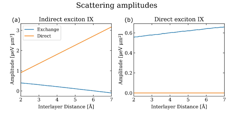
Supplementary Figure S10: Scattering amplitudes for exciton-exciton Coulomb interaction. (a,b) We show the change of scattering amplitudes with the interlayer distance. In (a), note the behavior of exchange scattering amplitude for indirect excitons, becoming negative past a threshold distance. Direct scattering amplitude grows linearly with distance. (b) We plot characteristic scattering amplitudes for direct excitons, where the direct process is zero at the negligible exchanged momentum (orange line), and the blue line corresponds to the exchange processes.

With direct excitons, we have $V^{\mathrm{dir}}_{\mathrm{X-X}}(\mathbf{q}=\mathbf{0})=0$, and

$$\begin{split}V^{\mathrm{exch}}_{\mathrm{X-X}}(\mathbf{q}=\mathbf{0})=&\left({2\over\pi}\right)^{2}{e^{2}\over 4\pi\epsilon\epsilon_{0}}\alpha_{D}\int dx\,dy\,d\theta{2\pi xy\over\delta(x,y,\theta)}\\ &{1\over(1+r_{\mathrm{0}}\delta(x,y,\theta)/\alpha_{\mathrm{D}})^{2}-(\delta(x,y,\theta)r_{\mathrm{0}}/\alpha_{\mathrm{D}})^{2}e^{-2\delta(x,y,\theta){d\over\alpha_{\mathrm{D}}}}}\cdot\\ &\left(1+{r_{\mathrm{0}}\over\alpha_{\mathrm{D}}}\left(1-e^{-2\delta(x,y,\theta){d\over\alpha_{\mathrm{D}}}}\right)\right)\cdot\biggl{(}{(-1)\over(1+x^{2})^{3}}{1\over(1+y^{2})^{3}}\\ &+{1\over(1+x^{2})^{3}}{e^{-\delta(x,y,\theta){d\over\alpha_{\mathrm{D}}}}\over(1+y^{2})^{3/2}(1+x^{2})^{3/2}}\biggr{)},\end{split}$$ (S12)

where $\delta(x,y,\theta)=\sqrt{x^{2}+y^{2}-2xy\cos{\theta}}$. With indirect excitons, the direct scattering amplitude recovers the capacitor formula $V^{\mathrm{dir}}_{\mathrm{I-I}}(\mathbf{q}=\mathbf{0})={e^{2}/(\epsilon\epsilon_{0}A)}d$, where $A$ is the sample area. Finally, the indirect exciton exchange potential has to be evaluated as

$$\begin{split}V^{\mathrm{exch}}_{\mathrm{I-I}}(\mathbf{q}=\mathbf{0})=&\left({2\over\pi}\right)^{2}{e^{2}\over 4\pi\epsilon\epsilon_{0}}\alpha_{D}\int dx\,dy\,d\theta{2\pi xy\over\delta(x,y,\theta)}\\ &{1\over(1+r_{\mathrm{0}}\delta(x,y,\theta)/\alpha_{\mathrm{I}})^{2}-(\delta(x,y,\theta)r_{\mathrm{0}}/\alpha_{\mathrm{I}})^{2}e^{-2\delta(x,y,\theta){d\over\alpha_{\mathrm{I}}}}}\cdot\\ &\biggl{[}{(-1)\over(1+x^{2})^{3}}{1\over(1+y^{2})^{3}}\left(1+{r_{\mathrm{0}}\over\alpha_{\mathrm{I}}}\left(1-e^{-2\delta(x,y,\theta){d\over\alpha_{\mathrm{I}}}}\right)\right)\\ &+{1\over(1+x^{2})^{3}}{e^{-\delta(x,y,\theta){d\over\alpha_{\mathrm{I}}}}\over(1+y^{2})^{3/2}(1+x^{2})^{3/2}}\biggr{]}.\end{split}$$ (S13)

Figs. S10(a) and (b) show the dependence of scattering amplitudes on the interlayer distance. We note the behavior of exchange scattering amplitude for indirect excitons, becoming negative past threshold distance (see Fig. S10(a)). Characteristically, for intralayer (i.e. direct) excitons we have a zero direct scattering amplitude, with non-zero contributions only due to the particle exchange process. With the estimated parameters, we find interlayer exciton-exciton interaction to have a scattering constant of $V_{\mathrm{I-I}}(\mathbf{q}=\mathbf{0})\simeq 2.5$ $\mu$eV $\mu$m², setting the scale for the Coulomb-based interactions.

Supplementary Note S12: Supplementary Note S9: Theory for energy shift

The out-of-cavity results (see Fig. 3 main text) reveal an opposite behavior of the sample response depending on the excitation regimes, where narrow bandwidth (NB) and the broad bandwidth (BB) regimes are considered. In the NB case, we observe a blueshift for the hIX peak, as already reported in literature for dipolar excitons [59, 60, 19], while in the BB regime we observe a redshifted signal. The latter is unexpected, as in the system with dipolar excitons and predominantly positive scattering matrix elements for exchange terms, the emergence of some effective attractive nonlinearities requires a new possible mechanism. Below, we motivate the emergence of such a mechanism unique to the bilayer system.

First, let us analyse the energy of system as the expectation value of the full Hamiltonian $\hat{\mathcal{H}}$. We consider electrons and holes distributed over bilayer as shown in Fig. 1(d) [main text]. We call $N_{\mathrm{I(D)}}$ the number of indirect (direct) excitons in the sample, and $n_{\mathrm{I(D)}}$ the particle density. The spin indices are omitted for brevity. The Hamiltonian of the system can be written as

$$\hat{\mathcal{H}}=\hat{\mathcal{H}}_{\mathrm{T}}+\hat{\mathcal{H}}_{\mathrm{sm}}+\hat{\mathcal{H}}_{\mathrm{df}},$$ (S14)

where $\hat{\mathcal{H}}_{\mathrm{T}}$ is the kinetic term, $\hat{\mathcal{H}}_{\mathrm{sm}}$ and $\hat{\mathcal{H}}_{\mathrm{df}}$ are the Coulomb interactions. With $\hat{\mathcal{H}}_{\mathrm{sm}}$ we refer to interacting particles belonging to a same band, and $\hat{\mathcal{H}}_{\mathrm{df}}$ corresponds to different dispersion bands. Explicitly, the kinetic energy reads

$$\hat{\mathcal{H}}_{\mathrm{T}}=\sum_{\mathbf{k}}\Big{[}\varepsilon_{c}^{t}(\mathbf{k})\hat{a}^{\dagger}_{\mathbf{k}}\hat{a}_{\mathbf{k}}+\varepsilon_{v}^{t}(\mathbf{k})b^{\dagger}_{\mathbf{k}}b_{\mathbf{k}}+\varepsilon_{c}^{b}(\mathbf{k})c^{\dagger}_{\mathbf{k}}c_{\mathbf{k}}\Big{]},$$ (S15)

where $\hat{a}^{\dagger}_{\mathbf{k}}$ and $\hat{b}^{\dagger}_{\mathbf{k}}$ are creation operators for conduction and valence bands of the top layer, respectively. $\hat{c}^{\dagger}_{\mathbf{k}}$ is an electron annihilation operator for the conduction band of the bottom layer. Each operator is labelled with a crystal momentum $\mathbf{k}$. $\varepsilon_{\mathrm{c(v)}}^{\mathrm{t(b)}}(\mathbf{k})$ are dispersions for conduction (valence) bands in the top (bottom) layer. The interactions are mediated through the Keldysh-Rytova potential. The corresponding interaction Hamiltonian reads

$$\hat{\mathcal{H}}_{\mathrm{sm}}=\frac{1}{2}\sum_{\mathbf{k},\mathbf{k}^{\prime},\mathbf{q}}\Big{[}V^{\mathrm{intra}}_{\mathrm{KR}}(\mathbf{q})(a^{\dagger}_{\mathbf{k}-\mathbf{q}}\hat{a}^{\dagger}_{\mathbf{k}^{\prime}+\mathbf{q}}\hat{a}_{\mathbf{k}^{\prime}}\hat{a}_{\mathbf{k}}+\hat{b}^{\dagger}_{\mathbf{k}-\mathbf{q}}\hat{b}^{\dagger}_{\mathbf{k}^{\prime}+\mathbf{q}}\hat{b}_{\mathbf{k}^{\prime}}\hat{b}_{\mathbf{k}}+c^{\dagger}_{\mathbf{k}-\mathbf{q}}\hat{c}^{\dagger}_{\mathbf{k}^{\prime}+\mathbf{q}}\hat{c}_{\mathbf{k}^{\prime}}\hat{c}_{\mathbf{k}})\Big{]},$$ (S16)

$$\hat{\mathcal{H}}_{\mathrm{df}}=\sum_{\mathbf{k},\mathbf{k}^{\prime},\mathbf{q}}\Big{[}V^{\mathrm{inter}}_{\mathrm{KR}}(\mathbf{q})(\hat{a}^{\dagger}_{\mathbf{k}-\mathbf{q}}\hat{c}^{\dagger}_{\mathbf{k}^{\prime}+\mathbf{q}}\hat{c}_{\mathbf{k}^{\prime}}\hat{a}_{\mathbf{k}}+\hat{b}^{\dagger}_{\mathbf{k}-\mathbf{q}}\hat{c}^{\dagger}_{\mathbf{k}^{\prime}+\mathbf{q}}\hat{c}_{\mathbf{k}^{\prime}}\hat{b}_{\mathbf{k}})+V^{\mathrm{intra}}_{\mathrm{KR}}\hat{a}^{\dagger}_{\mathbf{k}-\mathbf{q}}\hat{b}^{\dagger}_{\mathbf{k}^{\prime}+\mathbf{q}}\hat{b}_{\mathbf{k}^{\prime}}\hat{a}_{\mathbf{k}}\Big{]}.$$ (S17)

We define the exciton creation operators in the form

$$\hat{D}_{\mathrm{\mu}}^{\dagger}(\mathbf{Q})= \sum_{\mathbf{k}}\phi^{\mathrm{\mu}}_{\mathrm{D}}(\mathbf{k})\hat{a}^{\dagger}_{\mathbf{k}+\gamma_{\mathrm{e}}\mathbf{Q}}\hat{b}_{\mathbf{k}-\gamma_{\mathrm{h}}\mathbf{Q}},$$ (S18)

$$\hat{I}_{\mathrm{\nu}}^{\dagger}(\mathbf{P})= \sum_{\mathbf{k}}\phi^{\mathrm{\nu}}_{\mathrm{I}}(\mathbf{k})\hat{a}^{\dagger}_{\mathbf{k}+\gamma_{\mathrm{e}}\mathbf{P}}\hat{c}_{\mathbf{k}-\gamma_{\mathrm{h}}\mathbf{P}},$$ (S19)

with $\hat{D}^{\dagger}_{\mathrm{\mu}}(\mathbf{Q})$ [$\hat{I}^{\dagger}_{\mathrm{\nu}}(\mathbf{P})$] and $\phi^{\mathrm{\mu}}_{\mathrm{D}}(\mathbf{k})$ [$\phi^{\mathrm{\nu}}_{\mathrm{I}}(\mathbf{k})$] being the direct [indirect] exciton creation operator and wave function, respectfully. $\mathbf{Q},\mathbf{P}$ are crystal momenta, and $\mu,\nu$ are state indices. When we omit the $\mu$ and $\nu$ indices, and the total momentum, we refer the ground state at crystal momentum $\mathcal{Q}=0$. To take into account for particle non-bosonicity and consequent nonlinear behaviour, we consider the expectation value of a system over a multi-particle state created by exciting the vacuum state $|\Omega_{\mathrm{0}}\rangle$. It includes $N_{\mathrm{D}}$ direct excitons and $N_{\mathrm{I}}$ indirect excitons. The expectation $\langle\Omega_{\mathrm{0}}|\hat{D}^{N_{\mathrm{D}}}\hat{I}^{N_{\mathrm{I}}}\hat{\mathcal{H}}\hat{D}^{\dagger N_{\mathrm{D}}}\hat{I}^{\dagger N_{\mathrm{I}}}|\Omega_{\mathrm{0}}\rangle$ then denotes the total energy of the many-body system. By following a procedure for accounting non-bosonic correction at increasing order [43], we first commute the Hamiltonian with the product of exciton operators $\hat{D}^{\dagger N_{\mathrm{D}}}$, leading to

$$\begin{split}[\mathcal{H},\hat{D}^{\dagger N_{\mathrm{D}}}]=&N_{\mathrm{D}}E_{\mathrm{D}}\hat{D}^{\dagger N_{\mathrm{D}}-1}+N_{\mathrm{D}}\hat{D}^{\dagger N_{\mathrm{D}}-1}\hat{V}_{\mathrm{D}}\\ &+\frac{N_{\mathrm{D}}(N_{\mathrm{D}}-1)}{2}\hat{D}^{\dagger N_{\mathrm{D}}-2}\sum_{\mu,\nu,\mathrm{q}}V^{\mu,\nu}_{\mathrm{D-D}}(\mathbf{q})\hat{D}^{\dagger}_{\nu}(\mathbf{q})\hat{D}^{\dagger}_{\mu}(-\mathbf{q}),\end{split}$$ (S20)

where $V^{\mu,\nu}_{\mathrm{D-D}}(\mathbf{q})$ is the scattering matrix element of two direct excitons exchanging a momentum of $\mathbf{q}$. $\hat{V}_{\mathrm{D}}$ is the scattering potential [43], which arises from the commutator $[\mathcal{H},\hat{D}^{\dagger}]$ and is a signature of the phase space filling. Similarly, for indirect excitons we get

$${}\begin{split}[\mathcal{H},\hat{I}^{\dagger N_{\mathrm{I}}}]=&N_{\mathrm{I}}E_{\mathrm{I}}\hat{I}^{\dagger\mathrm{N}_{I}-1}+N_{\mathrm{I}}\hat{I}^{\dagger N_{\mathrm{I}}-1}\hat{V}_{\mathrm{I}}\\ &+\frac{N_{\mathrm{I}}(N_{\mathrm{I}}-1)}{2}\hat{I}^{\dagger\mathrm{N_{\mathrm{I}}-2}}\sum_{\mu,\nu,\mathrm{q}}V^{\mu,\nu}_{\mathrm{I-I}}(\mathbf{q})\hat{I}^{\dagger}_{\nu}(\mathbf{q})\hat{I}^{\dagger}_{\mu}(-\mathbf{q}),\end{split}$$ (S21)

with the notation being similar to Eq. (S20). We note the property of the scattering potential such that $\hat{V}_{\mathrm{D,I}}|\Omega_{0}\rangle=0$. With the given commutators, we can rewrite the total energy as

$$\begin{split}&\langle\Omega_{\mathrm{0}}|\hat{D}^{N_{\mathrm{D}}}\hat{I}^{N_{\mathrm{I}}}\hat{\mathcal{H}}\hat{D}^{\dagger N_{\mathrm{D}}}\hat{I}^{\dagger N_{\mathrm{I}}}|\Omega_{\mathrm{0}}\rangle=\\ &=N_{\mathrm{I}}E_{\mathrm{I}}\langle\Omega_{\mathrm{0}}|\hat{D}^{N_{\mathrm{D}}}\hat{I}^{N_{\mathrm{I}}}\hat{D}^{\dagger N_{\mathrm{D}}}\hat{I}^{\dagger N_{\mathrm{I}}}|\Omega_{\mathrm{0}}\rangle+N_{\mathrm{D}}E_{\mathrm{D}}\langle\Omega_{\mathrm{0}}|\hat{I}^{N_{\mathrm{I}}}\hat{D}^{N_{\mathrm{D}}}\hat{D}^{\dagger N_{\mathrm{D}}}\hat{I}^{\dagger N_{\mathrm{I}}}|\Omega_{\mathrm{0}}\rangle\\ &+\frac{N_{\mathrm{I}}(N_{\mathrm{I}}-1)}{2}\hat{I}^{\dagger N_{\mathrm{I}}-2}\sum_{\mu,\nu,\mathrm{q}}V^{\mu,\nu}_{\mathrm{I-I}}(\mathbf{q})\langle\Omega_{\mathrm{0}}|\hat{D}^{N_{\mathrm{D}}}\hat{I}^{N_{\mathrm{I}}}\hat{D}^{\dagger N_{\mathrm{D}}}\hat{I}^{\dagger N_{\mathrm{I}}-2}\hat{I}^{\dagger}_{\nu}(\mathbf{q})\hat{I}^{\dagger}_{\mu}(-\mathbf{q})|\Omega_{\mathrm{0}}\rangle\\ &+\frac{N_{\mathrm{D}}(N_{\mathrm{D}}-1)}{2}\hat{D}^{\dagger N_{\mathrm{D}}-2}\sum_{\mu,\nu,\mathrm{q}}V^{\mu,\nu}_{\mathrm{D-D}}(\mathbf{q})\langle\Omega_{\mathrm{0}}|\hat{D}^{N_{\mathrm{D}}}\hat{I}^{N_{\mathrm{I}}}\hat{D}^{\dagger N_{\mathrm{D}}-2}\hat{D}^{\dagger}_{\nu}(\mathbf{q})\hat{D}^{\dagger}_{\mu}(-\mathbf{q})\hat{I}^{\dagger N_{\mathrm{I}}}|\Omega_{\mathrm{0}}\rangle\\ &+N_{\mathrm{D}}N_{\mathrm{I}}\sum_{\mu,\nu,\mathbf{q}}V^{\mu,\nu}_{\mathrm{D-I}}(\mathbf{q})\langle\Omega_{\mathrm{0}}|\hat{D}^{N_{\mathrm{D}}}\hat{I}^{N_{\mathrm{I}}}\hat{D}^{\dagger N_{\mathrm{D}}-1}\hat{D}^{\dagger}_{\mu}(\mathbf{q})\hat{I}^{\dagger}_{\nu}(-\mathbf{q})\hat{I}^{\dagger N_{\mathrm{I}}-1}|\Omega_{\mathrm{0}}\rangle.\end{split}$$ (S22)

Eq. (S22) describes various energy contributions (linear and nonlinear) that are present in the system. We note that each term is proportional to the expectation value $\langle\Omega_{\mathrm{0}}|\hat{D}^{N_{\mathrm{D}}}\hat{I}^{N_{\mathrm{I}}}\hat{D}^{\dagger N_{\mathrm{D}}}\hat{I}^{\dagger N_{\mathrm{I}}}|\Omega_{\mathrm{0}}\rangle$, which deviates from $1$ due to the non-bosonicity of composite excitons. This reveals three possible creation potentials $\hat{V}^{\mu,\nu}_{\mathrm{D-D}},\hat{V}^{\mu,\nu}_{\mathrm{I-I}}$, and $\hat{V}^{\mu,\nu}_{\mathrm{D-I}}$, which noticeably generate cross-flavour interaction. The presence of creation potentials, as well as quadratic scaling of these terms in the total energy, is the signature of nonlinear behaviour. Terms in lines 2 and 3 of Eq. (S22) are the energy shifts for direct and indirect excitons due to phase space filling within the same exciton flavour. The last term in line 4 is the cross interaction of direct and indirect excitons, allowing for extra energy shifts in modes that are not statistically independent. Namely, the corresponding operators for intralayer and interlayer excitons do not commute as they share a hole, but formed by different electrons in conduction bands. This leads to the negative valued commutator, and here we identify the origin of unusual redshift, as observed in the work. We refer to this effect as hole crowding, where hole population being shared between the two different particles (hIX and X_A). This is different from statistical deviation of same excitons, where both carriers are exchanged, which we simply refer as interlayer exciton phase space filling, in analogy to the monolayer case. The effect of intra-flavour terms has already been discussed in Ref. [29], and leads to positive energy shifts. However, the cross-flavour terms only emerge in bilayers, and to date remained unexplored. We evaluate the considered term in $\mathbf{q}\simeq 0$, as it gives the dominant contribution observed in experiments, and we consider particles being in the ground state as a main occupation at low temperatures. With this, we rewrite the mutual energy shift $\Delta E_{\mathrm{I}}=\sum_{\mu,\nu,\mathbf{q}}V^{\mu,\nu}_{\mathrm{D-I}}(\mathbf{q})\langle\Omega_{\mathrm{0}}|\hat{D}^{N_{\mathrm{D}}}\hat{I}^{N_{\mathrm{I}}}\hat{D}^{\dagger N_{\mathrm{D}}-1}\hat{D}^{\dagger}_{\mu}(\mathbf{q})\hat{I}^{\dagger}_{\nu}(-\mathbf{q})\hat{I}^{\dagger N_{\mathrm{I}}-1}|\Omega_{\mathrm{0}}\rangle$ as

$$\Delta E_{\mathrm{I}}=-\xi\frac{e^{2}}{4\pi\epsilon\epsilon_{\mathrm{0}}A}\mathcal{I}\alpha,$$ (S23)

with $A$ being the sample area, and parameter $\xi$ of the order of unity, $\xi\sim 1$, is tuned to match with experimental data setting an effective area. Here, $\alpha=(\alpha_{\mathrm{D}}^{-1}+\alpha_{\mathrm{I}}^{-1})^{-1}$ is the reduced particle Bohr radius. The dimensionless exchange integral $\mathcal{I}$ has the form

$$\begin{split}\mathcal{I}=&\int d^{2}xd^{2}y\tilde{V}^{\mathrm{intra}}_{\mathrm{KR}}(|\mathbf{x}-\mathbf{y}|)\frac{1}{(1+\alpha_{1}^{2}x^{2})^{3/2}}\frac{1}{(1+\alpha_{2}^{2}y^{2})^{3}}\cdot\\ &\cdot\left(\frac{1}{(1+\alpha_{1}^{2}x^{2})^{3/2}}-\frac{1}{(1+\alpha_{2}^{2}y^{2})^{3/2}}\right)\\ &+\tilde{V}^{\mathrm{inter}}_{\mathrm{KR}}(|\mathbf{x}-\mathbf{y}|)\frac{1}{(1+\alpha_{2}^{2}y^{2})^{3/2}}\frac{1}{(1+\alpha_{1}^{2}y^{2})^{3/2}}\frac{1}{(1+\alpha_{2}^{2}x^{2})^{3/2}}\cdot\\ &\cdot\left(\frac{1}{(1+\alpha_{1}^{2}x^{2})^{3/2}}-\frac{1}{(1+\alpha_{1}^{2}y^{2})^{3/2}}\right),\end{split}$$ (S24)

where $\tilde{V}^{\mathrm{inter}}_{\mathrm{KR}}(|\mathbf{x}-\mathbf{y}|)$ is Keldysh-Rytova potential in dimensionless form, $\alpha_{\mathrm{1}}$ and $\alpha_{\mathrm{2}}$ are respectfully equal to $\alpha_{\mathrm{D}}/\alpha$ and $\alpha_{\mathrm{I}}/\alpha$. By estimating the exciton density as proportional to oscillator strength, we find $n_{\mathrm{I}}\simeq n_{\mathrm{D}}/4$. Numerically, we estimate the shift with $\epsilon=4$, $\alpha\simeq 6.7$ Å. The resulting shift can be estimated as $\Delta E_{\mathrm{I}}=-0.24\xi~{}\mu$eV $\mu$m${}^{2}\sqrt{n_{\mathrm{D}}n_{\mathrm{I}}}$.

References

- Deng et al. [2010] H. Deng, H. Haug, and Y. Yamamoto, Exciton-polariton Bose-Einstein condensation, Reviews of Modern Physics 82, 1489 (2010).
- Kasprzak et al. [2006] J. Kasprzak et al., Bose-Einstein condensation of exciton polaritons, Nature 443, 409 (2006).
- Christopoulos et al. [2007] S. Christopoulos et al., Room-temperature polariton lasing in semiconductor microcavities, Physical Review Letters 98, 126405 (2007).
- Bhattacharya et al. [2014] P. Bhattacharya et al., Room temperature electrically injected polariton laser, Physical Review Letters 112, 236802 (2014).
- Amo et al. [2009a] A. Amo et al., Collective fluid dynamics of a polariton condensate in a semiconductor microcavity, Nature 457, 291 (2009a).
- Liu et al. [2014] X. Liu, T. Galfsky, Z. Sun, F. Xia, E. C. Lin, Y. H. Lee, S. Kéna-Cohen, and V. M. Menon, Strong light-matter coupling in two-dimensional atomic crystals, Nature Photonics 9, 30 (2014).
- Dufferwiel et al. [2015] S. Dufferwiel, S. Schwarz, F. Withers, A. A. Trichet, F. Li, M. Sich, O. Del Pozo-Zamudio, C. Clark, A. Nalitov, D. D. Solnyshkov, G. Malpuech, K. S. Novoselov, J. M. Smith, M. S. Skolnick, D. N. Krizhanovskii, and A. I. Tartakovskii, Exciton-polaritons in van der Waals heterostructures embedded in tunable microcavities, Nature Communications 6, 1 (2015).
- Lundt et al. [2017] N. Lundt, A. Maryński, E. Cherotchenko, A. Pant, X. Fan, S. Tongay, G. Sek, A. V. Kavokin, S. Höfling, and C. Schneider, Monolayered MoSe2: A candidate for room temperature polaritonics, 2D Materials 4 (2017).
- Sidler et al. [2017] M. Sidler, P. Back, O. Cotlet, A. Srivastava, T. Fink, M. Kroner, E. Demler, and A. Imamoglu, Fermi polaron-polaritons in charge-tunable atomically thin semiconductors, Nature Physics 13, 255 (2017).
- Dufferwiel et al. [2017] S. Dufferwiel, T. P. Lyons, D. D. Solnyshkov, A. A. Trichet, F. Withers, S. Schwarz, G. Malpuech, J. M. Smith, K. S. Novoselov, M. S. Skolnick, D. N. Krizhanovskii, and A. I. Tartakovskii, Valley-addressable polaritons in atomically thin semiconductors, Nature Photonics 11, 497 (2017).
- Gerber et al. [2019] I. C. Gerber, E. Courtade, S. Shree, C. Robert, T. Taniguchi, K. Watanabe, A. Balocchi, P. Renucci, D. Lagarde, X. Marie, and B. Urbaszek, Interlayer excitons in bilayer MoS2 with strong oscillator strength up to room temperature, Physical Review B 99, 1 (2019).
- Leisgang et al. [2020] N. Leisgang, S. Shree, I. Paradisanos, L. Sponfeldner, C. Robert, D. Lagarde, A. Balocchi, K. Watanabe, T. Taniguchi, X. Marie, et al., Giant Stark splitting of an exciton in bilayer MoS2, Nature Nanotechnology 15, 901 (2020).
- Lorchat et al. [2021] E. Lorchat, M. Selig, F. Katsch, K. Yumigeta, S. Tongay, A. Knorr, C. Schneider, and S. Höfling, Excitons in bilayer mos 2 displaying a colossal electric field splitting and tunable magnetic response, Physical Review Letters 126, 037401 (2021).
- Peimyoo et al. [2021] N. Peimyoo, T. Deilmann, F. Withers, J. Escolar, D. Nutting, T. Taniguchi, K. Watanabe, A. Taghizadeh, M. F. Craciun, K. S. Thygesen, and S. Russo, Electrical tuning of optically active interlayer excitons in bilayer MoS2, Nature Nanotechnology 16, 888 (2021).
- Wilson et al. [2021] N. P. Wilson, W. Yao, J. Shan, and X. Xu, Excitons and emergent quantum phenomena in stacked 2d semiconductors, Nature 599, 383 (2021).
- Zhang et al. [2021] L. Zhang, F. Wu, S. Hou, Z. Zhang, Y.-H. Chou, K. Watanabe, T. Taniguchi, S. R. Forrest, and H. Deng, Van der waals heterostructure polaritons with moiré-induced nonlinearity, Nature 591, 61 (2021).
- Cristofolini et al. [2012] P. Cristofolini, G. Christmann, S. I. Tsintzos, G. Deligeorgis, G. Konstantinidis, Z. Hatzopoulos, P. G. Savvidis, and J. J. Baumberg, Coupling quantum tunneling with cavity photons, Science 336, 704 (2012).
- Togan et al. [2018] E. Togan, H.-T. Lim, S. Faelt, W. Wegscheider, and A. Imamoglu, Enhanced Interactions between Dipolar Polaritons, Phys. Rev. Lett. 121, 227402 (2018).
- Kyriienko et al. [2012] O. Kyriienko, E. B. Magnusson, and I. A. Shelykh, Spin dynamics of cold exciton condensates, Phys. Rev. B 86, 115324 (2012).
- Berloff et al. [2017] N. G. Berloff, M. Silva, K. Kalinin, A. Askitopoulos, J. D. Töpfer, P. Cilibrizzi, W. Langbein, and P. G. Lagoudakis, Realizing the classical xy hamiltonian in polariton simulators, Nature materials 16, 1120 (2017).
- Delteil et al. [2019] A. Delteil, T. Fink, A. Schade, S. Höfling, C. Schneider, and A. İmamoğlu, Towards polariton blockade of confined exciton–polaritons, Nature materials 18, 219 (2019).
- Kyriienko et al. [2020] O. Kyriienko, D. Krizhanovskii, and I. Shelykh, Nonlinear quantum optics with trion polaritons in 2d monolayers: conventional and unconventional photon blockade, Physical Review Letters 125, 197402 (2020).
- Wang et al. [2018] G. Wang, A. Chernikov, M. M. Glazov, T. F. Heinz, X. Marie, T. Amand, and B. Urbaszek, Colloquium: Excitons in atomically thin transition metal dichalcogenides, Reviews of Modern Physics 90, 21001 (2018), arXiv:1707.05863 .
- Lyons et al. [2021] T. P. Lyons, D. J. Gillard, C. Leblanc, J. Puebla, D. D. Solnyshkov, L. Klompmaker, I. A. Akimov, C. Louca, P. Muduli, A. Genco, M. Bayer, Y. Otani, G. Malpuech, and A. I. Tartakovskii, Giant effective Zeeman splitting in a monolayer semiconductor realized by spin-selective strong light-matter coupling, Arxiv (2021).
- Gillard et al. [2021] D. J. Gillard, A. Genco, S. Ahn, T. P. Lyons, K. Yeol Ma, A. R. Jang, T. Severs Millard, A. A. Trichet, R. Jayaprakash, K. Georgiou, D. G. Lidzey, J. M. Smith, H. Suk Shin, and A. I. Tartakovskii, Strong exciton-photon coupling in large area MoSe2 and WSe2 heterostructures fabricated from two-dimensional materials grown by chemical vapor deposition, 2D Materials 8 (2021).
- Gu et al. [2019] J. Gu, B. Chakraborty, M. Khatoniar, and V. M. Menon, A room-temperature polariton light-emitting diode based on monolayer WS2, Nature Nanotechnology 14, 1024 (2019).
- Lundt et al. [2019] N. Lundt, Ł. Dusanowski, E. Sedov, P. Stepanov, M. M. Glazov, S. Klembt, M. Klaas, J. Beierlein, Y. Qin, S. Tongay, et al., Optical valley hall effect for highly valley-coherent exciton-polaritons in an atomically thin semiconductor, Nature nanotechnology 14, 770 (2019).
- Tan et al. [2020] L. B. Tan, O. Cotlet, A. Bergschneider, R. Schmidt, P. Back, Y. Shimazaki, M. Kroner, and A. İmamoğlu, Interacting polaron-polaritons, Physical Review X 10, 021011 (2020).
- Emmanuele et al. [2020] R. Emmanuele, M. Sich, O. Kyriienko, V. Shahnazaryan, F. Withers, A. Catanzaro, P. Walker, F. Benimetskiy, M. Skolnick, A. Tartakovskii, et al., Highly nonlinear trion-polaritons in a monolayer semiconductor, Nature communications 11, 1 (2020).
- Gu et al. [2021] J. Gu, V. Walther, L. Waldecker, D. Rhodes, A. Raja, J. C. Hone, T. F. Heinz, S. Kéna-Cohen, T. Pohl, and V. M. Menon, Enhanced nonlinear interaction of polaritons via excitonic Rydberg states in monolayer WSe2, Nature Communications 12, 10.1038/s41467-021-22537-x (2021), arXiv:1912.12544 .
- Rivera et al. [2018] P. Rivera, H. Yu, K. L. Seyler, N. P. Wilson, W. Yao, and X. Xu, Interlayer valley excitons in heterobilayers of transition metal dichalcogenides, Nature nanotechnology 13, 1004 (2018).
- Butov [2004] L. V. Butov, Condensation and pattern formation in cold exciton gases in coupled quantum wells, Journal of Physics: Condensed Matter 16, R1577 (2004).
- Hubert et al. [2019] C. Hubert, Y. Baruchi, Y. Mazuz-Harpaz, K. Cohen, K. Biermann, M. Lemeshko, K. West, L. Pfeiffer, R. Rapaport, and P. Santos, Attractive dipolar coupling between stacked exciton fluids, Phys. Rev. X 9, 021026 (2019).
- Butov et al. [2002] L. Butov, A. Gossard, and D. Chemla, Macroscopically ordered state in an exciton system, Nature 418, 751 (2002).
- Fox et al. [1991] A. Fox, D. Miller, G. Livescu, J. Cunningham, and W. Jan, Excitonic effects in coupled quantum wells, Physical Review B 44, 6231 (1991).
- Alexeev et al. [2019a] E. M. Alexeev, D. A. Ruiz-Tijerina, M. Danovich, M. J. Hamer, D. J. Terry, P. K. Nayak, S. Ahn, S. Pak, J. Lee, J. I. Sohn, et al., Resonantly hybridized excitons in moiré superlattices in van der waals heterostructures, Nature 567, 81 (2019a).
- Paradisanos et al. [2020] I. Paradisanos, S. Shree, A. George, N. Leisgang, C. Robert, K. Watanabe, T. Taniguchi, R. J. Warburton, A. Turchanin, X. Marie, et al., Controlling interlayer excitons in MoS2 layers grown by chemical vapor deposition, Nature communications 11, 1 (2020).
- Amo et al. [2009b] A. Amo, D. Sanvitto, F. Laussy, D. Ballarini, E. d. Valle, M. Martin, A. Lemaitre, J. Bloch, D. Krizhanovskii, M. Skolnick, et al., Collective fluid dynamics of a polariton condensate in a semiconductor microcavity, Nature 457, 291 (2009b).
- Gong et al. [2013] Z. Gong, G. B. Liu, H. Yu, D. Xiao, X. Cui, X. Xu, and W. Yao, Magnetoelectric effects and valley-controlled spin quantum gates in transition metal dichalcogenide bilayers, Nature Communications 4, 1 (2013).
- Erkensten et al. [2021] D. Erkensten, S. Brem, and E. Malic, Exciton-exciton interaction in transition metal dichalcogenide monolayers and van der waals heterostructures, Phys. Rev. B 103, 045426 (2021).
- Shahnazaryan et al. [2017] V. Shahnazaryan, I. Iorsh, I. A. Shelykh, and O. Kyriienko, Exciton-exciton interaction in transition-metal dichalcogenide monolayers, Phys. Rev. B 96, 115409 (2017).
- Kristinsson et al. [2013] K. Kristinsson, O. Kyriienko, T. C. H. Liew, and I. A. Shelykh, Continuous terahertz emission from dipolaritons, Phys. Rev. B 88, 245303 (2013).
- Combescot et al. [2008] M. Combescot, O. Betbeder-Matibet, and F. Dubin, The many-body physics of composite bosons, Physics Reports 463, 215 (2008).
- Cappelluti et al. [2013] E. Cappelluti, R. Roldán, J. A. Silva-Guillén, P. Ordejón, and F. Guinea, Tight-binding model and direct-gap/indirect-gap transition in single-layer and multilayer mos2, Phys. Rev. B 88, 075409 (2013).
- Cudazzo et al. [2011] P. Cudazzo, I. V. Tokatly, and A. Rubio, Dielectric screening in two-dimensional insulators: Implications for excitonic and impurity states in graphane, Phys. Rev. B 84, 085406 (2011).
- Berkelbach et al. [2013] T. C. Berkelbach, M. S. Hybertsen, and D. R. Reichman, Theory of neutral and charged excitons in monolayer transition metal dichalcogenides, Physical Review B 88, 045318 (2013).
- Chernikov et al. [2014] A. Chernikov, T. C. Berkelbach, H. M. Hill, A. Rigosi, Y. Li, O. B. Aslan, D. R. Reichman, M. S. Hybertsen, and T. F. Heinz, Exciton binding energy and nonhydrogenic Rydberg series in monolayer WS2, Physical review letters 113, 076802 (2014).
- Danovich et al. [2018] M. Danovich, D. A. Ruiz-Tijerina, R. J. Hunt, M. Szyniszewski, N. D. Drummond, and V. I. Fal’ko, Localized interlayer complexes in heterobilayer transition metal dichalcogenides, Physical Review B 97, 195452 (2018).
- Kormányos et al. [2015] A. Kormányos, G. Burkard, M. Gmitra, J. Fabian, V. Zólyomi, N. D. Drummond, and V. Fal’ko, k· p theory for two-dimensional transition metal dichalcogenide semiconductors, 2D Materials 2, 022001 (2015).
- Alexeev et al. [2019b] E. M. Alexeev, D. A. Ruiz-Tijerina, M. Danovich, M. J. Hamer, D. J. Terry, P. K. Nayak, S. Ahn, S. Pak, J. Lee, J. I. Sohn, et al., Resonantly hybridized excitons in moiré superlattices in van der waals heterostructures, Nature 567, 81 (2019b).
- Savona et al. [1995] V. Savona, L. Andreani, P. Schwendimann, and A. Quattropani, Quantum well excitons in semiconductor microcavities: Unified treatment of weak and strong coupling regimes, Solid State Communications 93, 733 (1995).
- Din et al. [2021] N. U. Din, V. Turkowski, and T. S. Rahman, Ultrafast charge dynamics and photoluminescence in bilayer MoS2, 2D Materials 8, 025018 (2021).
- Nie et al. [2014] Z. Nie, R. Long, L. Sun, C.-C. Huang, J. Zhang, Q. Xiong, D. W. Hewak, Z. Shen, O. V. Prezhdo, and Z.-H. Loh, Ultrafast carrier thermalization and cooling dynamics in few-layer MoS2, ACS nano 8, 10931 (2014).
- Palummo et al. [2015] M. Palummo, M. Bernardi, and J. C. Grossman, Exciton radiative lifetimes in two-dimensional transition metal dichalcogenides, Nano letters 15, 2794 (2015).
- Wang et al. [2015] H. Wang, C. Zhang, and F. Rana, Ultrafast dynamics of defect-assisted electron–hole recombination in monolayer MoS2, Nano letters 15, 339 (2015).
- Hughes and Hase [2010] I. Hughes and T. Hase, Measurements and their uncertainties: a practical guide to modern error analysis (OUP Oxford, 2010).
- Ivchenko et al. [1996] E. Ivchenko, M. Kaliteevski, A. Kavokin, and A. Nesvizhskii, Reflection and absorption spectra from microcavities with resonant bragg quantum wells, JOSA B 13, 1061 (1996).
- Ciuti et al. [1998] C. Ciuti, V. Savona, C. Piermarocchi, A. Quattropani, and P. Schwendimann, Role of the exchange of carriers in elastic exciton-exciton scattering in quantum wells, Physical Review B 58, 7926 (1998).
- Schindler and Zimmermann [2008] C. Schindler and R. Zimmermann, Analysis of the exciton-exciton interaction in semiconductor quantum wells, Physical Review B 78, 045313 (2008).
- Zimmermann and Schindler [2007] R. Zimmermann and C. Schindler, Exciton–exciton interaction in coupled quantum wells, Solid state communications 144, 395 (2007).