Supplementary Materials
Temporal coherence of optical fields in the presence of entanglement

I Classical Mach-Zehnder interferometer (MZI) with optical filter

To compare the results of classical and quantum interferometers, we consider an unbalanced classical Mach-Zehnder interferometer (MZI) for a train of pulses input to the interferometer, as shown in Fig.1. The pulse train is described by

$$E(t)=\sum_{j}E_{j}(t-j\Delta T)$$ (1)

with $E_{j}(t)\equiv A_{j}h(t)$ for the single $j$-th pulse with amplitude $A_{j}$ and the same normalized shape $h(t)$ $(\int dt|h(t)|^{2}=1)$ for all pulses. The width of $h(t)$ is denoted as $\delta t$. Denote $h(\omega)\equiv\int dth(t)e^{-i\omega t}$ as the Fourier component of $h(t)$. With the paths of the two arms unbalanced by a relative delay of $L/c$, the field at the output of the MZI is

$$E_{out}(t) \propto E(t)+E(t+L/c)$$ (2)

$$= \sum_{j}E_{j}(t-j\Delta T)+E_{j}(t+L/c-j\Delta T)$$ (3)

Now let us place an optical filter of amplitude transmissivity $f(\omega)$ at the output of the interferometer. The field after the filter is then

$$E_{out}^{\prime}(t)=\sum_{j}E_{j}^{\prime}(t-j\Delta T)+E_{j}^{\prime}(t+L/c-j\Delta T)~{}~{}~{}~{}$$ (4)

with $E_{j}^{\prime}(t)\equiv A_{j}h^{\prime}(t)$. $h^{\prime}(t)$, whose Fourier component is $h^{\prime}(\omega)=h(\omega)f(\omega)$, is the new pulse shape after the filter with a width of $\delta t^{\prime}$. For the simplicity of argument, we assume that $\delta t^{\prime},L/c<\Delta T$, that is, there is no overlap between different pulses in the pulse train even after filtering. With this assumption, it is straightforward to find the intensity after the filter as

$$I_{out}^{\prime}(t) = \sum_{j}|E_{j}^{\prime}(t-j\Delta T)|^{2}+|E_{j}^{\prime}(t+\frac{L}{c}-j\Delta T)|^{2}$$ (6)

$$+\sum_{j}{E_{j}^{\prime}}^{*}(t-j\Delta T)E_{j}^{\prime}(t+\frac{L}{c}-j\Delta T)+c.c.~{}~{}~{}~{}$$

For a detector with a response function of $k(\tau)$ whose width is the resolution time $T_{R}$, the photo-current of the detector for the filtered field is

$$i_{D}(t) = \int d\tau k(t-\tau)I_{out}^{\prime}(\tau).$$ (7)

For a slow detector that cannot resolve shape of a single pulse, its time resolution $T_{R}\gg\delta t^{\prime}$. Then Eq.(7) can be approximated as

$$i_{D}(t) \approx \sum_{j}k(t-j\Delta T)|A_{j}|^{2}\int d\tau\Big{[}|h^{\prime}(\tau)|^{2}$$ (9)

$$\hskip 21.68121pt+|h^{\prime}(\tau+L/c)|^{2}+{h^{\prime}}^{*}(\tau)h^{\prime}(\tau+L/c)+c.c.\Big{]}$$

$$= 2Q(t)(1+{\cal V}_{M}\cos\Delta\varphi),$$ (10)

with $Q(t)\equiv\sum_{j}k(t-j\Delta T)|A_{j}|^{2}\int d\tau|h^{\prime}(\tau)|^{2}$, visibility ${\cal V}_{M}(L/c)\equiv|\int d\tau{h^{\prime}}^{*}(\tau)h^{\prime}(\tau+L/c)|$ $/\int d\tau|h^{\prime}(\tau)|^{2}$ and phase $\Delta\varphi\equiv{\rm Arg}[\int d\tau{h^{\prime}}^{*}(\tau)h^{\prime}(\tau+L/c)]$.

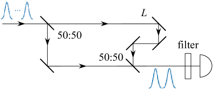
Figure 1: An unbalanced Mach-Zehnder interferometer (MZI) with filtered detection.

Take a Gaussian shape for both the initial pulse and the filter: $h(\omega)=e^{-(\omega-\omega_{0})^{2}/2\sigma^{2}}$, $f(\omega)=e^{-(\omega-\omega_{0})^{2}/2\sigma_{f}^{2}}$, which gives $h(t)$ $=e^{-t^{2}/2\delta t^{2}}$, $h^{\prime}(t)$ $=e^{-t^{2}/2{\delta t^{\prime}}^{2}}$ with $\delta t=$ $1/\sigma$ and ${\delta t^{\prime}}=\sqrt{1/\sigma^{2}+1/\sigma_{f}^{2}}$ , we find ${\cal V}_{M}(\Delta)=$ $e^{-\Delta^{2}/4{T_{c}^{\prime}}^{2}}$ $(\Delta\equiv L/c)$ with

$${T_{c}^{\prime}}^{2}\equiv{T_{c}^{\prime}}^{2}+T_{f}^{2}={\delta t^{\prime}}^{2},$$ (11)

where $T_{f}\equiv 1/\sigma_{f}$. Here, $\delta t={T_{c}}$ and $\delta t^{\prime}={T_{c}^{\prime}}$ are the pulse widths or coherence time of the initial and filtered pulses, respectively. So, if the delay $\Delta=L/c\gg\delta t$, no interference occurs without optical filtering ($\sigma_{f}=\infty$ and $T_{f}=1/\sigma_{f}=0$). But the interference can be recovered with ${\cal V}\approx 100\%$ if the filter is narrow enough so that $T_{c}^{\prime}$ is much larger than the delay $\Delta=L/c$. The filter lengthens the coherence time of the pulses so that they will overlap at the BS and interfere. This is consistent with the coherence time concept in classical coherence theory.

II The calculation of concurrence for entangled photon pairs

The states of entangled photon pairs produced from the experiment in main text is in general of the form

$$|\Psi\rangle=e^{i\phi}\sqrt{f}|s_{1}\rangle\otimes|i_{1}\rangle+\sqrt{1-f}|s_{2}\rangle\otimes|i_{2}\rangle,$$ (12)

where $\sqrt{f}\equiv|A_{1}|$ and $\sqrt{1-f}\equiv|A_{2}|$ are related to the pump fields of PA1 and PA2, respectively. Since $\langle{s_{1}}|{s_{2}}\rangle=0$ and $\langle{i_{1}}|{i_{2}}\rangle\neq 0$ (with $0\leq f\leq 1$, $0\leq\phi\leq 2\pi$) , state $|s_{1}\rangle$ is found to be orthonormal to $|s_{2}\rangle$, while states $|i_{1}\rangle$ and $|i_{2}\rangle$ are not. In order to find a certain state $|u\rangle$ which is orthonormal to state $|i_{1}\rangle$, one can make decomposition of the state $|i_{2}\rangle=\cos{\theta}|i_{1}\rangle+\sin{\theta}|u\rangle$, with $0\leq\theta\leq\frac{\pi}{2}$. Note that any extra phase between $|i_{1}\rangle$ and $|i_{2}\rangle$ can be absorbed in $e^{i\phi}$ and in state $|u\rangle$. The state in Eq.(12) thus reads

$$|\Psi\rangle= e^{i\phi}\sqrt{f}|s_{1}\rangle\otimes|i_{1}\rangle+\sqrt{1-f}\cos{\theta}|{s_{2}}\rangle\otimes|i_{1}\rangle$$ (13)

$$+\sqrt{1-f}\sin{\theta}|s_{2}\rangle\otimes|u\rangle.$$

Having the entangled state in the new orthonormal basis ($|s_{1}\rangle\otimes|i_{1}\rangle,|s_{2}\rangle\otimes|i_{1}\rangle,|s_{2}\rangle\otimes|u\rangle,|s_{1}\rangle\otimes|u\rangle$), and defining the Pauli matrices

$$\begin{split}&\sigma_{z}^{s}=|s_{2}\rangle\langle s_{2}|-|s_{1}\rangle\langle{s_{1}}|,\\ &\sigma_{z}^{i}=|i_{1}\rangle\langle{i_{1}}|-|u\rangle\langle{u}|.\end{split}$$

Furthermore, one can find $\sigma_{y}^{s}$ and $\sigma_{y}^{i}$ and obtain $\sigma_{y}^{s}\otimes\sigma_{y}^{i}$

$$\begin{split}\sigma_{y}^{s}\otimes\sigma_{y}^{i}=&-(|{s_{2},i_{1}}\rangle\langle{s_{1},u}|-|{s_{2},u}\rangle\langle{s_{1},i_{1}}|\\ &-|{s_{1},i_{1}}\rangle\langle{s_{2},u}|+|{s_{1},u}\rangle\langle{s_{2},i_{1}})|\\ =&\begin{pmatrix}0&0&1&0\\ 0&0&0&-1\\ 1&0&0&0\\ 0&-1&0&0\end{pmatrix}.\end{split}$$ (14)

The density operator reads

$$\rho=|{\psi}\rangle\langle{\psi}|=\begin{pmatrix}f&e^{i\phi}\sqrt{(1-f)f}\cos{\theta}&e^{i\phi}\sqrt{(1-f)f}\sin{\theta}&0\\ e^{-i\phi}\sqrt{(1-f)f}\cos{\theta}&(1-f)\cos^{2}{\theta}&(1-f)\cos{\theta}\sin{\theta}&0\\ e^{-i\phi}\sqrt{(1-f)f}\sin{\theta}&(1-f)\cos{\theta}\sin{\theta}&(1-f)\sin^{2}{\theta}&0\\ 0&0&0&0\end{pmatrix}.$$ (15)

The spin-flipped state $\tilde{\rho}$ can be found in Ref. 1 and is written as

$$\tilde{\rho} =(\sigma_{y}^{s}\otimes\sigma_{y}^{i})\rho^{*}(\sigma_{y}^{s}\otimes\sigma_{y}^{i})$$ (16)

$$=\begin{pmatrix}0&0&e^{-i\phi}\sqrt{(1-f)f}\sin{\theta}&0\\ 0&0&0&0\\ e^{i\phi}\sqrt{(1-f)f}\sin{\theta}&0&0&0\\ 0&0&0&0\end{pmatrix},$$

where $\rho^{*}$ is the complex conjugation of $\rho$. Then it is easy to find the Hermitian matrix

$$R= \sqrt{\sqrt{\rho}\tilde{\rho}\sqrt{\rho}}$$ (17)

$$= \begin{pmatrix}0&0&\sqrt{(1-f)f\sin^{2}{\theta}}&0\\ 0&0&0&0\\ \sqrt{(1-f)f\sin^{2}{\theta}}&0&0&0\\ 0&0&0&0\end{pmatrix}.$$

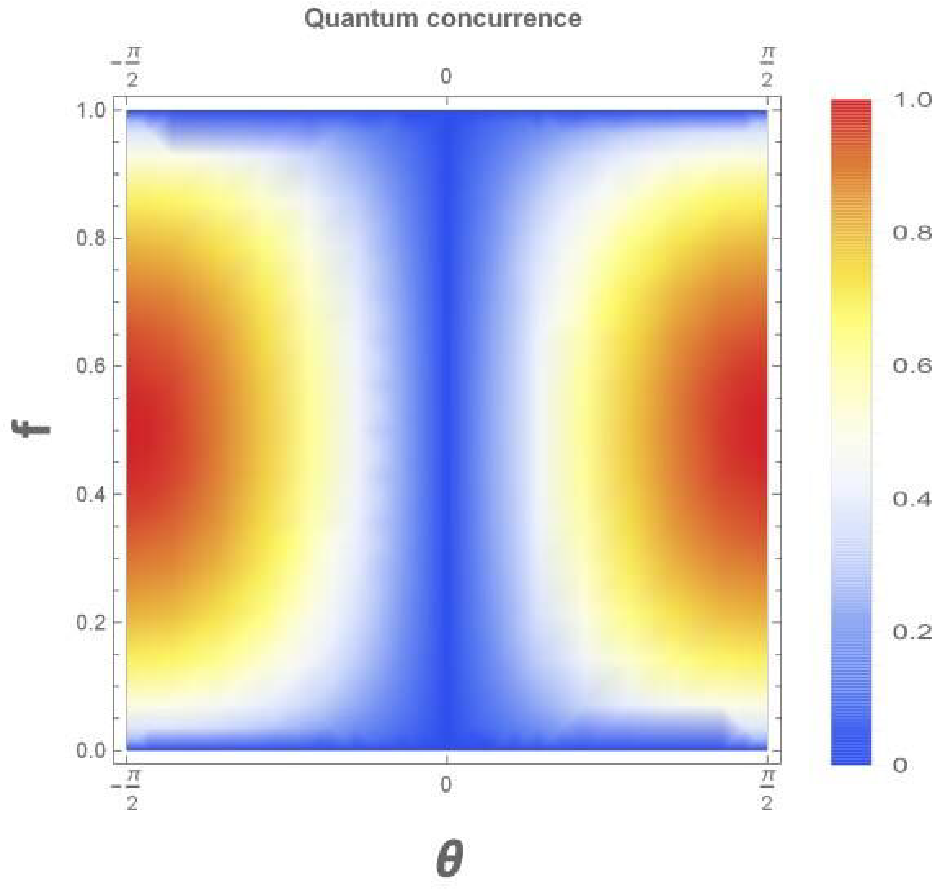
Figure 2: Quantum concurrence of the entangled photon pairs state as a function of parameter $\theta$ and $f$.

Having the eigenvalues of matrix R: $[\lambda_{1},\lambda_{2},\lambda_{3},\lambda_{4}]$= $[\sqrt{(1-f)f\sin^{2}{\theta}},0,0,-\sqrt{(1-f)f\sin^{2}{\theta}}]$ in decreasing order. The concurrence for a mixed state of two qubits has been derived by Wootters [1], can be expressed in terms of the parameters $\theta$ and $f$

$$C(\theta,f) =max(0,\lambda_{1}-\lambda_{2}-\lambda_{3}-\lambda_{4})$$ (18)

$$=max(0,2\sqrt{(1-f)f}|\sin{\theta}|),$$

Alternatively, one can also define a non-Hermitian matrix to solve the matrix

$$R_{a}=\rho\tilde{\rho}=\begin{pmatrix}0&0&(1-f)f\sin^{2}{\theta}&0\\ 0&0&0&0\\ (1-f)f\sin^{2}{\theta}&0&0&0\\ 0&0&0&0\end{pmatrix}.$$

The real eigenvalues are thus given in decreasing order: $[\alpha_{1},\alpha_{2},\alpha_{3},\alpha_{4}]=[(1-f)f\sin^{2}{\theta},0,0,-(1-f)f\sin^{2}{\theta}]$ and obtain $\lambda_{i}=\sqrt{\alpha_{i}}$. The concurrence can be eventually solved by

$$C(\theta,f) =max(0,\sqrt{\alpha_{1}}-\sqrt{\alpha_{2}}-\sqrt{\alpha_{3}}-\sqrt{\alpha_{4}})$$ (19)

$$=max(0,2\sqrt{(1-f)f}|\sin{\theta}|),$$

which reproduces Eq.(18) from Hermitian matrix.

Figure 2 plots the result of Eq.(18) as well as Eq.(19).

III Limiting case of $\sigma_{f}\rightarrow 0$ for the multi-mode description

In this case, we have

$$f_{s}(\Omega_{1})\Phi(\Omega_{1},\Omega_{2})$$ (20)

$$\hskip 14.45377pt=\exp\bigg{(}-\frac{\Omega_{1}^{2}}{2\sigma_{f}^{2}}\bigg{)}\exp\bigg{[}-\frac{(\Omega_{1}+\Omega_{2})^{2}}{4\sigma_{p}^{2}}-\frac{(\Omega_{1}-\Omega_{2})^{2}}{2\sigma_{0}^{2}}\bigg{]}$$ (21)

$$\hskip 14.45377pt\approx\exp\bigg{(}-\frac{\Omega_{1}^{2}}{2\sigma_{f}^{2}}\bigg{)}\exp\bigg{[}-\frac{\Omega_{2}^{2}}{2}\Big{(}\frac{1}{2\sigma_{p}^{2}}+\frac{1}{\sigma_{0}^{2}}\Big{)}\bigg{]}$$ (22)

if $\sigma_{f}\ll\sigma_{p},\sigma_{0}$. Then the factorized states for the idler fields are

$$|i_{1}\rangle = \int d\Omega\phi(\Omega)\hat{a}_{i}^{{\dagger}}(\Omega)|vac\rangle$$ (23)

$$|i_{2}\rangle = \int d\Omega\phi(\Omega)e^{i\Omega\Delta_{i}}\hat{a}_{i}^{{\dagger}}(\Omega)|vac\rangle$$ (24)

with $\phi(\Omega)\equiv N\exp\bigg{[}-\frac{\Omega_{2}^{2}}{2}\Big{(}\frac{1}{2\sigma_{p}^{2}}+\frac{1}{\sigma_{0}^{2}}\Big{)}\bigg{]}$. From these two states, we obtain

$$\cos\theta \equiv \langle i_{1}|i_{2}\rangle=\int d\Omega|\phi(\Omega)|^{2}e^{i\Omega\Delta_{i}}$$ (25)

$$= \exp\bigg{(}-\Delta_{i}^{2}/4\bar{T}_{i}^{2}\bigg{)}$$ (26)

with $\bar{T}_{i}^{2}\equiv\frac{1}{2\sigma_{p}^{2}}+\frac{1}{\sigma_{0}^{2}}$

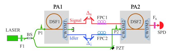
Figure 3: Experimental setup. BS, 50/50 beam splitter; CWDM, coarse wavelength division multiplexer; DSF, dispersion shifted fiber; F, filter; P, pump; PA, parametric amplifier; PZT, piezoelectric transducer; SPD, single photon detector.

IV Details of the experimental arrangement and procedures

IV.1 Experimental setup

The experimental setup of our SU(1,1) interferometer is shown in Fig. 3. The two PAs are based on four-wave mixing (FWM) in dispersion-shifted fibers (DSF). The pumps of two PAs (P1 and P2) are obtained by passing the output of a femoto-second fiber laser through a band pass filter (F1) and 50/50 beam splitter (BS). The repetition rate of laser is about 50 MHz. PA1 consists of a DSF and a coarse wavelength division multiplexer (CWDM); while PA2 consists of a DSF and two CWDMs. The two DSFs with zero-dispersion wavelength and length of 1548.5 nm and 150 m, respectively, are identical. The central wavelength of the pumps (P1 and P2) is set at 1549.3 nm, and the pulse width (or bandwidth) of two pumps can be varied within the range of about $3$-$15$ ps ($0.2$-$0.8$ nm ) by adjusting F1. Under this condition, the phase matching condition of FWM with a gain bandwidth up to 25 nm in both signal and idler bands is achieved in DSFs. The course wavelength division multiplexers (CWDMs) having three channels for pump, signal, and idler fields, respectively, are used for the separation or combination of fields at different wavelengths.

The entangled signal and idler fields are generated in PA1 via spontaneous FWM. The two entangled fields are separated from P1 by CWDM1 and propagate along different paths. CWDM2 couples pump P2 and signal and idler fields into DSF2, and CWDM3 separates signal and idler output fields from P2. In the experiment, the production rate of signal and idler photon pairs is about 0.1 pairs/pulse/nm in PA1. The delays relative to the time slot of pump pulse ($\Delta_{s}$ and $\Delta_{i}$) are introduced to the signal and idler arms for an unbalanced interferometer. In PA2, the mode overlap of all fields involved in FWM is optimized by adjusting the fiber polarization controllers (FPC1 and FPC2) in signal and idler arms to maximize the visibility [2]. When the SU(1,1) interferometer is balanced, i.e., $\Delta_{s}=\Delta_{i}=0$, the visibility is the highest. With the increase of the delays, the visibility decreases.

With the intention to lengthen the coherence time of the detected field and erase the temporal distinguishability for recovering the interference at the output, a narrow optical filter (F_s) is placed at the signal output port. The power of filtered signal field is measured by an InGaAs-based single photon detector (SPD, Langyan SPD4V5) operated in a gated Geiger mode. The 2.5-ns gate pulses coincide with the arrival of photons at SPDs. The response time of SPDs is about 1 ns, which is 100 times longer than the pulse duration of the detected field. The interference pattern is measured when the phase of the pump P2 is varied by scanning a piezoelectric transducer at about 0.8 Hz and the integration time of SPD is set to 20 ms.

In our experimental setup, the transmission efficiencies for the idler and signal arms between two PA2 are $56\%$ and $64\%$, respectively, because there exist transmission loss of CWDMs, fusion loss between fibers and coupling loss induced by delay lines. Since the transmission loss in each DSF is negligibly small, the ratio between the powers of P2 and P1 is adjusted to $P_{2}/P_{1}=0.6$. In this case, time-bin entangled state with maximum entanglement （$A_{1}=A_{2}$） can be obtained [4]. For each CWDM, the 1 dB bandwidth of each channel is 16 nm, and the wavelength separation of adjacent channels is 20 nm. So the equivalent 3 dB bandwidth of correlated signal and idler fields launched into DSF2 is about 10 nm (1.25 THz), which is a combined spectral effect of the FWM gain and CWDM pass bands. As a result, the value of $\sigma_{0}$ in Eqs. (14) should be substituted for this equivalent bandwidth (about 4.8 rad/ps). The bandwidth of the filter (F_s) is controlled by using a programmable optical filter (WS, Finisar 4000S), whose central wavelength is fixed at 1566.5 but the 3 dB bandwidth can be flexibly adjusted from 0.02 to 1 THz.

IV.2 Procedure for obtaining normalized visibility

During the experiment, the 3 dB bandwidth of pump is first set at 0.6 nm. Both the counting rate of SPD and voltage applied on PZT are recorded and analyzed by using a data acquisition system. The blue solid circles in Fig. 4(a) present a typical set of interference pattern when the delays in two arms of the SU(1,1) interferometer are zero ($\Delta_{s}=\Delta_{i}=0$) and the phase of the pump P2 is varied by scanning the PZT. Ideally, the visibility should be 100$\%$. However, because of the nonideal transmission between the two PAs and the existence of background Raman scattering in each DSF [3], the visibility in Fig. 4(a) is only about 60$\%$ [4]. With the increase of $\Delta_{s}$ and $\Delta_{i}$, the visibility will further decreases.

In principle, by correcting the directly observed interference pattern with the background noise induced by Raman scattering and transmission loss inside the SU(1,1) interferometer [4], 100$\%$ visibility is obtainable when $\Delta_{s}=\Delta_{i}=0$. Considering our goal here is to reveal dependence of time constants (T_s and T_i) of the field passing through filter F_s, the key is to describe how the visibility varies with the delays $\Delta_{s}$ and $\Delta_{i}$. Hence, the loss and Raman scattering induced non-ideal visibility (see Fig. 4(a)) will not affect the evaluation of T_s and T_i. This is similar to the technique in characterizing the coherence time of an optical field by using a Mach-Zehnder interferometer, whose maximum visibility deviates from 100$\%$ due to the unequal intensities in two arms.

In the experiment, we record the interference patterns for $\Delta_{s}$ and $\Delta_{i}$ with different values. Instead of carefully characterizing the amount of background noise to correct the raw data of interference, we normalize the observed visibility V_o with V_max, which is directly observed under the condition of $\Delta_{s}=\Delta_{i}=0$. As an example, Fig. 4(b) presents the normalized visibility ($V=V_{o}/V_{max}$) as a function of delay $\Delta_{s}$ when the delay $\Delta_{i}$ is fixed at 0 and the 3 dB bandwidth of filter F_s is 0.05, 0.1, and 0.5 THz, respectively. By collecting the normalized visibility for F_s with different bandwidths when the delays are $\Delta_{i}=0$, $\Delta_{s}=10$ ps, trace (i) (blue squares) in Fig. 1 of the main text is then acquired. The other two traces in Fig. 1 are obtained by collecting the normalized visibility obtained under the conditions of $\Delta_{s}=10$, $\Delta_{i}=5$ ps and $\Delta_{s}=\Delta_{i}=10$ ps, respectively.

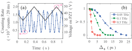
Figure 4: (a) The directly observed interference pattern when the phase of the pump P2 is varied by scanning the voltage applied on PZT and $\Delta_{s}=\Delta_{i}=0$. (b) The normalized visibility as a function of delay $\Delta_{s}$ when $\Delta_{i}=0$ and the 3 dB bandwidth of filter (Fs) is 0.05, 0.1 and 0.5 THz, respectively.

IV.3 Procedure for deducing time constants T_s and T_i

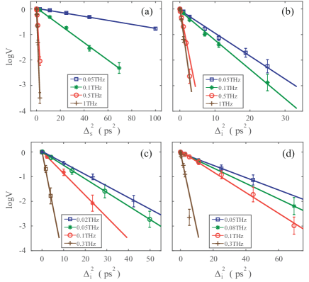
Figure 5: The normalized visibility as a function of (a) $\Delta_{s}^{2}$ with $\Delta_{i}=0$ and (b,c,d) $\Delta_{i}^{2}$ with $\Delta_{s}=0$ for F_s having different bandwidths as indicated in legends when the 3 dB bandwidth of pump is 0.24, 0.6 and 0.8 nm, respectively.

From the normalized visibility obtained under the condition of $\Delta_{i}=0$ (see Fig. 4(b)), we extract the time constant T_s by using Eq. (15) and fitting data to a linear regression of $\log V$ vs. $\Delta_{s}^{2}$, as shown in Fig. 5(a). Similarly, by using Eq. (18), we can extract the time constant T_i by changing $\Delta_{i}$ and fixing $\Delta_{s}$ at 0 when bandwidth of the filter F_s takes different values, as shown in Fig. 5(c). Moreover, we repeat the measurement of T_s and T_i by changing the 3 dB bandwidth of pump to 0.24 nm and 0.8 nm, respectively. We find there is no observable change in the deduced value of T_s when the pump bandwidth is altered. However, as shown in Fig. 5(b) and (d), T_i varies with the pump bandwidth. According to the best fit in Fig. 5, the four traces in Fig. 3 of the main text are obtained.

References

References

- [1] William K. Wootters, “Entanglement of Formation of an Arbitrary State of Two Qubits,” Phys. Rev. Lett. 80, 2245 (1998).
- [2] X. Guo, X. Li, N. Liu, and Z. Y. Ou, “Quantum information tapping using a fiber optical parametric amplifier with noise figure improved by correlated input,” Sci. Rep. 6, 30214 (2016).
- [3] X. Li, J. Chen, P. Voss, J. E. Sharping, and P. Kumar, “All-fiber photon-pair source for quantum communications: Improved generation of correlated photons,” Opt. Express 12, 3737 (2004).
- [4] L. Cui, J. Wang, J. Li, M. Ma, Z. Y. Ou, and X. Li, “Programmable photon pair source,” APL Photonics 7, 016101 (2022).