Estimating Separable Matching Models

Abstract

In this paper we propose two simple methods to estimate models of matching with transferable and separable utility introduced in [6] (cupid:restud). The first method is a minimum distance estimator that relies on the generalized entropy of matching. The second relies on a reformulation of the more special but popular [5] (choo-siow:06) model; it uses generalized linear models (GLMs) with two-way fixed effects.

Keywords: matching, marriage, assignment, estimations comparison.
JEL codes: C78, C13, C15.

Introduction

The estimation of models of two-sided matching has made considerable progress in the past decade. While some of this work has used matching under non-transferable utility, many applications have focused on markets where utility is transferable. The pioneering contribution of [5] (choo-siow:06) introduced a simple and highly tractable specification. They used their model to estimate the effect of the 1973 liberalization of abortion in the US on marriage outcomes. In doing so, they used a nonparametric estimator of the matching patterns. Their specification is a natural extension of the multinomial logit model, and it has become quite popular.

The [5] specification rests on three main assumptions that will be defined later in the paper: separability; large market; and standard type I extreme value random utility. In [6] (cupid:restud), we showed that the third, distributional assumption is not necessary: for any (separable) distribution of the errors, the joint surplus is nonparametrically identified. The nonparametric estimator of [5] was feasible in their case as they only conditioned on the ages of the partners in a couple. It breaks down, however, when more covariates are considered as matching cells become too small; and by construction, it does not allow for parameterized error distributions. Structural models of household behavior also naturally introduce parameters.

In all of these cases, the analyst must resort to parametric models. This note shows two very simple methods to estimate parametric versions of separable matching models with perfectly transferable utility, with special emphasis on the [5] model and more generally on “semilinear” models, where the joint surplus is linear in the parameters (again, to be formally defined later in the paper).

Our first method applies a minimum-distance estimator to the identification equation derived in [6] (cupid:restud), which relates the joint surplus to the derivatives of a generalized entropy function evaluated at the observed matching patterns. For any fixed distribution of the error terms, the generalized entropy can be evaluated and differentiated, numerically if needed. The estimator selects parameter values and also provides a simple specification test. In semilinear models, the estimator can be obtained in closed form.

The second method we present applies more specifically to the semilinear Choo and Siow model. We show that the moment-matching estimator we described in [6] (cupid:restud) can be reframed as a generalized linear model, more specifically as the pseudo-maximum likelihood estimator of a Poisson regression with two-sided fixed effects. This is available as linear_model in the scikit-learn library in Python, as fepois in the R package fixest and as ppmlhdfe in Stata, among other common statistical packages.

We conclude with a brief discussion of the pros and cons of these two methods. Both are coded in a Python package called cupid_matching that is available on the standard repositories.

1 The Model

This paper applies to a bipartite matching market with perfectly transferable utility. For simplicity, we refer to potential partners as “men” and “women”. We use the same notation as in [6] (cupid:restud). We assume that the analyst can only observe which of a finite set of types each individual belongs to. Men and women of a given type differ along some dimensions that they all observe, while the analyst does not. Each man $i\in\mathcal{I}$ belongs to one group of (observable) type $x_{i}\in\mathcal{X}$; and, similarly, each woman $j\in\mathcal{J}$ belongs to one (observable) type $y_{j}\in\mathcal{Y}$. We will say that “man $i$ is of type $x$” and “woman $j$ is of type $y$.” We denote $\mu_{ij}$ the indicator function for a matching between man $i$ and woman $j$, which is equal to $1$ if $i$ and $j$ are matched and to $0$ otherwise. Similarly, $\mu_{i0}$ and $\mu_{0j}$ are the indicator of $i$ or $j$ to remain unmatched, respectively. Without loss of generality, we assimilate $\mathcal{X}$ to $\{1,\ldots,X\}$ and $\mathcal{Y}$ to $\{1,\ldots,Y\}$. As $\mathcal{X}$ and $\mathcal{Y}$ will later serve as choice sets of partners types for women and men, respectively, and as the marital options needs to include remaining unmatched, we shall add the option to remain unmatched $0$ to these sets and denote $\mathcal{X}_{0}=\mathcal{X}\cup\{0\}$ and $\mathcal{Y}_{0}=\mathcal{Y}\cup\{0\}$ the respective sets of marital options of women and men.

We denote $n_{x}$ the mass of men of type $x\in\mathcal{X}$, and $m_{y}$ the mass of women of type $y\in\mathcal{Y}$. We denote $\bm{q}=(\bm{n},\bm{m})$ the vector that collects the margins $\bm{n}$ and $\bm{m}$ of the problem

In addition to the margins $\bm{q}$, the analyst observes matchings at the type level. We denote $\mu_{xy}$ the mass of the couples where the man belongs to type $x$, and where the woman belongs to type $y$, which is formally defined as $\mu_{xy}=\sum_{i\in\mathcal{I},j\in\mathcal{J}}\mu_{ij}1\{x_{i}=x\}1\{y_{j}=y\}$. We also denote $\mu_{x0}=\sum_{i\in\mathcal{I}}\mu_{i0}1\{x_{i}=x\}$, and $\mu_{0y}=\sum_{j\in\mathcal{J}}\mu_{0j}1\{y_{j}=y\}$ the mass of single individuals who are respectively men of type $x$ and women of type $y$. We will be interested in the limiting market with a large number of men in any type $x$, and of women in any type $y$. Since the problem is homogeneous, we shall normalize the total mass $N$ of households to one; that is, we rescale $\bm{\mu}$ and $\bm{q}$ by a multiplicative factor $N$ such that $\sum_{x,y}\mu_{xy}+\sum_{x}\mu_{x0}+\sum_{y}\mu_{0y}=1$. Again, we use the boldface notation $\bm{\mu}$ to denote the vector of matching numbers. We denote $\mathcal{A}=\mathcal{X}\times\mathcal{Y}\cup\mathcal{X}\times\{0\}\cup\{0\}\times\mathcal{Y}$ the set of possible marital arrangements (matched household of type $xy$, or single households of type $x0$ or $0y$), so that $\bm{\mu}$ is a vector of $\mathbb{R}^{\mathcal{A}}$.

A matching is the specification of who matches with whom. It is feasible if each individual is matched to at most one partner. It is stable if no individual who has a partner would prefer to be single, and if no two individuals would prefer forming a couple over their current situation.

We model the joint surplus $\tilde{\Phi}_{ij}$, which is the sum of the cardinal utilities that both a man $i$ and a woman $j$ jointly obtain by being matched together, and we assume a separable matching surplus:

Assumption 1 (Separability).

There exist a vector $\bm{\Phi}$ in $\mathrm{I\kern-1.69998ptR}^{X\times Y}$ and random terms $\bm{\varepsilon}$ and $\bm{\eta}$ such that

• the joint utility from a match between a man $i$ of type $x\in\mathcal{X}$ and a woman $j$ of type $y\in\mathcal{Y}$ is

  $$\tilde{\Phi}_{ij}=\Phi_{xy}+\varepsilon_{iy}+\eta_{xj},$$ (1.1)

• the utility of a single man $i$ is $\tilde{\Phi}_{i0}=\varepsilon_{i0}$,

• the utility of a single woman $j$ is $\tilde{\Phi}_{0j}=\eta_{0j}$,

where, conditional on $x_{i}=x$, the random vector $\bm{\varepsilon}_{i}=(\varepsilon_{iy})_{y\in\mathcal{Y}_{0}}$ has probability distribution $\mathbb{P}_{x}$, and, conditional on $y_{j}=y$, the random vector $\bm{\eta}_{j}=(\eta_{xj})_{x\in\mathcal{X}_{0}}$ has probability distribution $\mathbb{Q}_{y}$. The distributions $\mathbb{P}_{x}$ and $\mathbb{Q}_{y}$ have full support and a density with respect to the Lebesgue measure. The variables

$$\max_{y\in\mathcal{Y}_{0}}\;\lvert\varepsilon_{iy}\rvert\;\mbox{ and }\;\max_{x\in\mathcal{X}_{0}}\;\lvert\eta_{xj}\rvert$$

have finite expectations under $\mathbb{P}_{x}$ and $\mathbb{Q}_{y}$ respectively.

Separability allows for a restricted form of “matching on unobservables”; it rules out interaction terms on characteristics that are unobserved on both sides of the market, e.g. some unobserved preference of man $i$ for some unobserved characteristics of woman $j$.

[4] (csw:17) and [6] (cupid:restud) showed that under separability, at any stable matching $\bm{\mu}$ there exist two matrices $\bm{U}$ and $\bm{V}$ such that for all $(x,y)$, $U_{xy}+V_{xy}=\Phi_{xy}$, and $U_{x0}=V_{0y}=0$, and such that man $i$ of type $x$ is assigned option $y=0,1,\ldots,Y$ which maximizes $U_{xy}+\varepsilon_{iy}$ (where option $0$ means remaining unmatched, and option $y\neq 0$ means being matched with a woman of type $y$); similarly woman $j$ of type $y$ is assigned option $x=0,1,\ldots,X$ which maximizes $V_{xy}+\eta_{xj}$.

1.1 Generalized Entropy

Consider the classic “Emax” function $G_{x}$ defined as follows. In this paragraph we let $\bm{U}=(U_{1},\ldots,U_{Y})$ be a $Y$-dimensional vector. Then we define

$$G_{x}(\bm{U})=E_{\mathbb{P}_{x}}\max\left(\max_{y\in\mathcal{Y}}(U_{y}+\varepsilon_{iy}),\varepsilon_{i0}\right).$$

As a maximum of linear functions, $G_{x}$ is a convex function. We denote $\partial G_{x}(\bm{U})$ its subgradient; because of the assumptions made on $\mathbb{P}_{x}$, it is a singleton almost everywhere.

Now take the Legendre-Fenchel transform of $G_{x}$: for any $(\nu_{1},\ldots,\nu_{Y})$ such that $\sum_{y\in\mathcal{Y}}\nu_{y}\leq 1$, we define

$$G^{\ast}_{x}(\bm{\nu})=\max_{\bm{U}}\left(\sum_{y\in\mathcal{Y}}\nu_{y}U_{y}-G_{x}(\bm{U})\right).$$

It is another convex function; and since $G_{x}$ is convex, $G_{x}$ is the Legendre-Fenchel transform of $G^{\ast}_{x}$. As a consequence,

$$\bm{\nu}\in\partial G_{x}(\bm{U})\;\mbox{if and only if}\;\bm{U}\in\partial G^{\ast}_{x}(\bm{\nu}).$$

This convex duality is at the core of the identification and inference results in [6] (cupid:restud).

Defining $H_{y}$ and $H^{\ast}_{y}$ in the same way, we get the generalized entropy: for any feasible matching $\bm{\mu}$,

$$\mathcal{E}(\bm{\mu},\bm{q})=-\sum_{x\in\mathcal{X}}n_{x}G^{\ast}_{x}\left(\frac{\bm{\mu}_{x\cdot}}{n_{x}}\right)-\sum_{y\in\mathcal{Y}}m_{y}H^{\ast}_{y}\left(\frac{\bm{\mu}_{\cdot y}}{m_{y}}\right).$$ (1.2)

The function $\mathcal{E}$ only depends on the matching patterns $\bm{\mu}$ and the margins $\bm{q}=(\bm{n},\bm{m})$. It is concave; its shape depends on the distributions $(\mathbb{P}_{x})$ and $(\mathbb{Q}_{y})$ of the unobserved heterogeneity terms $\bm{\varepsilon}$ and $\bm{\eta}$.

1.2 The Data

We assume that the analyst observes a random sample of size $N$ from a large population of households. By simple counting (possibly using sampling weights), she obtains estimators of the matching patterns $\hat{\mu}_{xy},\hat{\mu}_{x0}$, and $\hat{\mu}_{0y}$, as well as the margins:

$$\hat{n}_{x} =\hat{\mu}_{x0}+\sum_{y\in\mathcal{Y}}\hat{\mu}_{xy}$$

$$\hat{m}_{y} =\hat{\mu}_{0y}+\sum_{x\in\mathcal{X}}\hat{\mu}_{xy}$$

and a consistent estimator $\Sigma_{\hat{\bm{\mu}}}$ of their asymptotic variance-covariance matrix, given by

$$\Sigma_{\hat{\bm{\mu}}}=\text{diag}(\hat{\bm{\mu}})-\hat{\bm{\mu}}\hat{\bm{\mu}}^{\top}.$$

2 Minimum-distance Estimation

Recall that we have assumed that each $\mathbb{P}_{x}$ (resp. each $\mathbb{Q}_{y}$) has full support on $\mathrm{I\kern-1.69998ptR}^{Y+1}$ (resp. $\mathrm{I\kern-1.69998ptR}^{X+1}$). Then all $\mu_{xy},\mu_{x0},\mu_{0y}$ must be positive; as a consequence, the $G_{x},H_{y},G^{\ast}_{x},H^{\ast}_{y}$ functions are continuously differentiable everywhere, as is the generalized entropy function $\mathcal{E}$.

[6] (cupid:restud) showed that at the stable matching $\bm{\mu}$, the joint surplus matrix $\bm{\Phi}$ can be obtained by the following simple formula:

$$\Phi_{xy}=-\frac{\partial\mathcal{E}}{\partial\mu_{xy}}(\bm{\mu},\bm{q}).$$ (2.1)

These are the first-order conditions of the maximization of the total joint surplus

$$\mathcal{W}=\max_{\bm{\mu}}\left(\sum_{x,y}\mu_{xy}\Phi_{xy}+\mathcal{E}(\bm{\mu},\bm{q})\right).$$

Suppose that the distributions $\mathbb{P}_{x}$ and $\mathbb{Q}_{y}$ are specified up to a parameter vector $\bm{\alpha}\in\mathbb{R}^{d_{\bm{\alpha}}}$, while the joint surplus matrix $\bm{\Phi}$ is specified up to a parameter vector $\bm{\beta}\in\mathbb{R}^{d_{\bm{\beta}}}$. We write the generalized entropy function $\mathcal{E}^{\bm{\alpha}}$ and the parameterized surplus vector $\bm{\Phi}^{\bm{\beta}}$. Then one can use (2.1) as the basis for a minimum distance estimator. That is, we write a mixed hypothesis as

$$\exists\bm{\lambda}=(\bm{\alpha},\bm{\beta}),\;\;\bm{D}^{\bm{\lambda}}(\bm{\mu},\bm{q})\equiv\bm{\Phi}^{\bm{\beta}}+\frac{\partial\mathcal{E}^{\bm{\alpha}}}{\partial\bm{\mu}}(\bm{\mu},\bm{q})=\bm{0},$$

stacking all $X\times Y$ conditions in (2.1) in a vector $\bm{D}^{\bm{\lambda}}$.

We choose $\hat{\bm{\lambda}}$ to minimize $\lVert\bm{D}^{\bm{\lambda}}(\bm{\hat{\mu}},\bm{\hat{q}})\rVert^{2}_{\bm{S}}$ for some positive definite $(X\times Y,X\times Y)$ matrix $\bm{S}$. By the general theory of minimum distance estimators, we know that this yields a consistent estimator of $\bm{\lambda}$ if the model is well specified, and that if we choose $\bm{S}=\bm{\hat{\Omega}}^{-1}$ where $\bm{\hat{\Omega}}$ consistently estimates $V\bm{D}^{\bm{\lambda}}(\bm{\hat{\mu}},\bm{\hat{q}})$ (and can be obtained by the delta method), the minimum distance estimator will reach its efficiency bound. Further, if the model is well specified and the choice of $\bm{S}$ is the efficient one, the minimized value of the squared norm follows a $\chi^{2}$ of degree $X\times Y-d_{\bm{\alpha}}-d_{\bm{\beta}}$. Note that this optimization problem is not a convex optimization problem in general.

2.1 The Linear Case

Minimum-distance estimation is a particularly appealing strategy if both the derivatives of the generalized entropy function $\mathcal{E}^{\bm{\alpha}}$ and the surplus matrix $\bm{\Phi}^{\bm{\beta}}$ are linear in the parameters:

$$\frac{\partial\mathcal{E}^{\bm{\alpha}}}{\partial\mu_{xy}}(\bm{\mu},\bm{q})=e^{0}_{xy}(\bm{\mu},\bm{q})+e_{xy}(\bm{\mu},\bm{q})\cdot\bm{\alpha}$$ (2.2)

and

$$\Phi_{xy}^{\bm{\beta}}=\bm{\phi}_{xy}\cdot\bm{\beta}$$ (2.3)

for some vectors of basis functions $\bm{e}(\bm{\mu},\bm{q})$ and $\bm{\phi}$. Then

$$D_{xy}^{\bm{\lambda}}(\bm{\mu},\bm{q})=\bm{\phi}_{xy}\cdot\bm{\beta}+e^{0}_{xy}(\bm{\mu},\bm{q})+e_{xy}(\bm{\mu},\bm{q})\cdot\bm{\alpha}$$

is linear in the parameters $\bm{\lambda}$. (Recall that, for every $(x,y)\in\mathcal{X}\times\mathcal{Y}$, the vector $e_{xy}(\bm{\mu},\bm{q})$ is of size $d_{\bm{\alpha}}$, and $\bm{\phi}_{xy}$ is of size $d_{\bm{\beta}}$.)

These two conditions call for several remarks. Condition (2.3) is a natural choice for a flexible specification. Condition (2.2) trivially holds in models where the $\mathbb{P}_{x}$ and $\mathbb{Q}_{y}$ are parameter-free, like the ubiquitous [5] (choo-siow:06) specification. As we will see, it holds in several other leading examples. Note also that the parameter-free part $\bm{e}^{0}$ is necessary in order to normalize the scale of the error terms, which is otherwise not identified in this discrete-choice model.

Under conditions (2.2) and (2.3), the minimum distance estimator can be implemented by linear least-squares. Let $\bm{\hat{F}}$ denote the $(X\times Y,d_{\bm{\alpha}}+d_{\bm{\beta}})$ matrix that stacks $\bm{e}(\bm{\hat{\mu}},\bm{\hat{q}})$ and $\bm{\phi}$ vertically, so that $\bm{D}^{\lambda}(\bm{\hat{\mu}},\bm{\hat{r}})=\bm{\hat{e}}^{0}+\bm{\hat{F}}\bm{\lambda}$, where $\bm{\hat{e}}^{0}=\bm{e}^{0}(\bm{\hat{\mu}},\bm{\hat{q}})$ Then for any choice of $\bm{S}$, the minimum distance estimator $\bm{\hat{\lambda}}$ solves the linear system

$$\left(\bm{\hat{F}}^{\top}\bm{S}\bm{\hat{F}}\right)\;\hat{\bm{\lambda}}=-\bm{\hat{F}}^{\top}\bm{S}\bm{\hat{e}}^{0}.$$ (2.4)

Since $\bm{\hat{e}}^{0}$ and $\bm{\hat{F}}$ are functions of $(\bm{\hat{\mu}},\bm{\hat{q}})$, the variance $\bm{\hat{\Omega}}(\bm{\lambda})$ of $\bm{\hat{D}}^{\bm{\lambda}}$ can be computed from $\bm{\hat{V}}$ using the delta method. Again, taking $\bm{S}$ to be the inverse of $\bm{\hat{\Omega}}(\bm{\hat{\lambda}})$ is the efficient choice. This procedure is summarized in Box 1.

If the distributions $(\mathbb{P}_{x})$ and $(\mathbb{Q}_{y})$ are parameter-free, the matrix $\bm{\Omega}^{\ast}$ does not depend on $\bm{\lambda}$ any more, and $\bm{\hat{F}}$ is simply the matrix $\bm{\phi}$. The estimators of $\bm{\lambda}=\bm{\beta}$ can be obtained following the procedure described in Box 2.

Note that since $\bm{\phi}$ is non-random, the variance of $\bm{\hat{D}}^{\bm{\lambda}}$ is the variance of the derivative of the generalized entropy. Step 2 therefore requires evaluating the second derivatives of the generalized entropy $\mathcal{E}$: by the delta method,

$$V\bm{\hat{D}}^{\bm{\lambda}}=\begin{pmatrix}\mathcal{E}_{\bm{\mu}\bm{\mu}}^{\top}&\mathcal{E}_{\bm{\mu}\bm{q}}^{\top}\end{pmatrix}V\begin{pmatrix}\bm{\hat{\mu}}\\ \bm{\hat{q}}\end{pmatrix}\begin{pmatrix}\mathcal{E}_{\bm{\mu}\bm{\mu}}\\ \mathcal{E}_{\bm{\mu}\bm{q}}\end{pmatrix}.$$

It is easy to see from the definition in (1.2) that the first derivative of $\mathcal{E}$ with respect to $\mu_{xy}$ only depends on the conditional matching patterns $\mu_{\cdot|x}=(\mu_{x1}/n_{x},\ldots,\mu_{xY}/n_{x})$ of men of type $x$, and on those of women of type $y$. As a consequence, the Hessians of $\mathcal{E}$ are very sparse and are often easy to evaluate.

2.2 Examples

We start with two examples for which the generalized entropy and its derivatives are available in closed form; in both cases, the derivatives are linear in the parameters $\bm{\alpha}$. In our third example, the calculation requires finding the fixed point of a contraction, in a way that is familiar from empirical industrial organization.

2.2.1 The Heteroskedastic Logit Model

Let us start with an easy extension of the [5] (choo-siow:06) logit model: the distributions $\mathbb{P}_{x}$ and $\mathbb{Q}_{y}$ are type I-EV iid vectors with unknown scale factors $\sigma_{x}$ and $\tau_{y}$ respectively. Then $\bm{\alpha}=(\bm{\sigma},\bm{\tau})$ and the derivatives of the generalized entropy function are linear in $\bm{\alpha}$:

$$\frac{\partial\mathcal{E}^{\bm{\alpha}}}{\partial\mu_{xy}}(\bm{\mu},\bm{q})=-\sigma_{x}\log\frac{\mu_{xy}}{\mu_{x0}}-\tau_{y}\log\frac{\mu_{xy}}{\mu_{0y}}$$

where $\mu_{x0}=n_{x}-\sum_{y\in\mathcal{Y}}\mu_{xy}$ and $\mu_{0y}=m_{y}-\sum_{x\in\mathcal{X}}\mu_{xy}$. The second derivatives of the generalized entropy take a very simple form:

$$\frac{\partial^{2}\mathcal{E}^{\bm{\alpha}}}{\partial\mu_{xy}\partial\mu_{zt}}(\bm{\mu},\bm{q})=-\frac{\sigma_{x}}{\mu_{x0}}\;\mathrm{1\kern-3.99994pt1}(z=x)-\frac{\tau_{y}}{\mu_{0y}}\;\mathrm{1\kern-3.99994pt1}(t=y)-\frac{\sigma_{x}+\tau_{y}}{\mu_{xy}}\;\mathrm{1\kern-3.99994pt1}(z=x,t=y)$$ (2.5)

and

$$\frac{\partial^{2}\mathcal{E}^{\bm{\alpha}}}{\partial\mu_{xy}\partial n_{z}}(\bm{\mu},\bm{q})=\frac{\sigma_{x}}{\mu_{x0}}\;\mathrm{1\kern-3.99994pt1}(z=x);\;\;\;\;\;\frac{\partial^{2}\mathcal{E}^{\bm{\alpha}}}{\partial\mu_{xy}\partial m_{t}}(\bm{\mu},\bm{q})=\frac{\tau_{y}}{\mu_{0y}}\;\mathrm{1\kern-3.99994pt1}(t=y).$$ (2.6)

Scale normalization is done by fixing the value of one of the parameters in $\bm{\alpha}$. The [5] homoskedastic model obtains when all $\sigma_{x}$ and $\tau_{y}$ equal one; a gender-heteroskedastic model would have all $\sigma_{x}$ equal to one and all $\tau_{y}$ equal to an unknown $\tau$. [4] (csw:17) applied a minimum distance estimator to the homoskedastic and heteroskedastic logit models.

2.2.2 Nested Logit

Consider a two-layer nested logit model. Take men of type $x$ first. Alternative $0$ (singlehood) is obviously special; we put it alone in its nest. Each other nest $n\in\mathcal{N}_{x}$ contains alternatives $y\in\mathcal{Y}_{n}$. The correlation of alternatives within nest $n$ is proxied by $1-\left(\rho^{x}_{n}\right)^{2}$ (with $\rho^{x}_{0}=1$ for the nest made of alternative $0$). Similarly, for women of type $y$, alternative $0$ is in a nest by itself with parameter $\delta^{y}_{0}=1$ and alternatives $x\in\mathcal{X}_{n^{\prime}}$ are in a nest $n\in\mathcal{N}^{\prime}_{y}$ with parameter $\delta^{y}_{n^{\prime}}$. We collect the parameters $\bm{\rho}$ and $\bm{\delta}$ into $\bm{\alpha}$.

The formulæ in Example 2.1 of [6] (cupid:restud) imply that if $y$ is in nest $n\in\mathcal{N}_{x}$ and $x$ is in nest $n^{\prime}\in\mathcal{N}_{y}$, then

$$\frac{\partial\mathcal{E}^{\bm{\alpha}}}{\partial\mu_{xy}}(\bm{\mu},\bm{q}) =-\rho^{x}_{n}\log\frac{\mu_{xy}}{\mu_{x0}}-(1-\rho^{x}_{n})\log\frac{\mu_{xn}}{\mu_{x0}}$$

$$-\delta^{y}_{n^{\prime}}\log\frac{\mu_{xy}}{\mu_{0y}}-(1-\delta^{y}_{n^{\prime}})\log\frac{\mu_{n^{\prime}y}}{\mu_{0y}},$$ (2.7)

where we defined $\mu_{xn}=\sum_{t\in\mathcal{Y}_{n}}\mu_{xt}$ and $\mu_{n^{\prime}y}=\sum_{z\in\mathcal{X}_{n^{\prime}}}\mu_{zy}$. Once again, this is linear in the parameters $\bm{\alpha}$; it remains linear if we impose constraints on the nests (for instance, that $\mathcal{N}_{x}$ is the same for all types $x$) and/or linear constraints on the $\bm{\rho}$ parameters (for instance, that $\rho_{xn}$ only depends on $n$).

2.2.3 Mixed Logit

Let us now describe a random coefficient logit model. Consider a man $i$ of type $x$, endowed with preferences $\bm{e}_{i}$ over a set of $d$ observable characteristics $\bm{Z}$ of potential partners. We add an idiosyncratic shock $\bm{\zeta}_{i}$ that is distributed as a standard iid type I extreme value vector over $\mathrm{I\kern-1.69998ptR}^{Y+1}$, independently of $\bm{e}_{i}$, and a scale factor $s>0$:

$$\varepsilon_{iy}=\sum_{k=1}^{d}Z_{yk}e_{ik}+s\zeta_{iy}$$

or in matrix form: $\bm{\varepsilon}=\bm{Z}\bm{e}+s\bm{\zeta}$. This specification is standard in empirical IO. In [1] (blp:1995): the covariates in $\bm{Z}$ stand for the observed characteristics of the products; the $\bm{e}$ are individual valuations of these characteristics, and the $\bm{\zeta}$ are idiosyncratic shocks.

Let individual preferences $\bm{e}$ of men of type $x$ have distribution $\mathbb{P}^{e}_{x}$. We will seek to estimate the parameters $\bm{\beta}$ of the joint surplus, the scale factor $s$, and the parameters of the distributions $\mathbb{P}^{e}_{x}$. We collect $s$ and the parameters of $\mathbb{P}^{e}_{x}$ in a vector $\bm{\alpha}$.

To compute the derivative of the generalized entropy function, we recall from [6] (cupid:restud) that

$$G^{\ast}_{x}(\bm{\nu};\bm{\alpha})=-\min_{U_{0}=0,\bm{U}\in\mathbb{R}^{Y}}\left[\int s\log\sum_{y=0,1,\ldots,Y}\exp\left(\frac{U_{y}+\left(\bm{Z}\bm{e}\right)_{y}}{s}\right)d\mathbb{P}^{e}_{x}(\bm{e})-\sum_{y\in\mathcal{Y}}\nu_{y}U_{y}\right].$$

By the envelope theorem, the derivative of $G^{\ast}_{x}(\bm{\nu};\bm{\alpha})$ with respect to $\bm{\nu}$ is the vector $\bm{U}$ that solves the system

$$\nu_{y}=\int\frac{\exp((U_{y}+\bm{Z}_{y}\bm{e})/s)}{\sum_{t=0,1,\ldots,Y}\exp((U_{t}+\bm{Z}_{t}\bm{e})/s)}d\mathbb{P}^{e}_{x}(\bm{e})\;\;\forall y=1,\ldots,Y.$$

This is exactly isomorphic to the inversion problem in [1] (blp:1995), with the unknown $\bm{U}$ standing for the product effects and $\bm{\nu}$ playing the role of the product market shares. After replacing $\bm{\nu}$ with the observed $\bm{\mu}_{x\cdot}/n_{x}$, the system can be solved by any of the algorithms that are standard in this literature. The solution gives row $x$ of the matrix $\bm{U}$. Proceeding in the same way for other types of men, and solving for $\bm{V}$ for women, gives the derivatives of the generalized entropy function:

$$\frac{\partial\mathcal{E}^{\bm{\alpha}}}{\partial\mu_{xy}}(\bm{\mu},\bm{q})=-\frac{\partial G^{\ast}_{x}}{\partial\nu_{xy}}\left(\frac{\bm{\mu}_{x\cdot}}{n_{x}}\right)-\frac{\partial H^{\ast}_{y}}{\partial\nu_{xy}}\left(\frac{\bm{\mu}_{\cdot y}}{m_{y}}\right)=-U_{xy}-V_{xy}.$$

The limit case $s=0$ yields the pure characteristics model of [2] (berrypakes:07). Then the system to be solved for row $x$ of $\bm{U}$ is

$$\nu_{y}=\mathbb{P}^{e}_{x}\left(y\in\arg\max_{t=0,1,\ldots,Y}(U_{t}+\bm{Z}_{t}\bm{e})\right)\;\;\forall y=1,\ldots,Y.$$

If each $\bm{Z}_{t}$ is a scalar, the inequalities boil down to

$$e^{-}(y;\bm{U},\bm{Z})\equiv\max_{t|Z_{t}<Z_{y}}\frac{U_{t}-U_{y}}{Z_{y}-Z_{t}}\leq e\leq\min_{t|Z_{t}>Z_{y}}\frac{U_{y}-U_{t}}{Z_{t}-Z_{y}}\equiv e^{+}(y;\bm{U},\bm{Z}),$$

and the system of equations to be solved for $\bm{U}$ is

$$\nu_{y}=\mathbb{P}^{e}_{x}(e^{+}(y;\bm{U},\bm{Z}))-\mathbb{P}^{e}_{x}(e^{-}(y;\bm{U},\bm{Z}))\;\;\forall y=1,\ldots,Y.$$

3 Moment-based Estimation by Poisson Regression

Now take the generalized entropy function $\mathcal{E}$ as known/assumed; and assume that the joint surplus vector $\bm{\Phi}\in\mathbb{R}^{\mathcal{X}\times\mathcal{Y}}$ is semilinear: $\bm{\Phi}^{\bm{\beta}}=\bm{\phi}\bm{\beta}$, where $\bm{\beta}$ is a vector of dimension $d_{\bm{\beta}}$ and $\phi$ is a $|\mathcal{X}||\mathcal{Y}|\times d_{\bm{\beta}}$ matrix. [6] (cupid:restud) introduced a moment-matching procedure that gives a consistent estimator of the parameter vector $\bm{\beta}$ if the model is well-specified. The moment matching estimator equalizes the observed and simulated comoments, that is the expectations of the basis functions $\bm{\phi}$ under the observed and simulated matching patterns:

$$\sum_{x,y}\hat{\mu}_{xy}\bm{\phi}_{xy}=\sum_{x,y}\mu^{\bm{\beta}}_{xy}\bm{\phi}_{xy},$$

where $\bm{\mu}^{\bm{\beta}}$ denotes the stable matching patterns for the parameter vector $\bm{\beta}$. As explained in [6] (cupid:restud), these are the first-order conditions of the following maximization problem:

$$\max_{\bm{\beta}}\left(\bm{\hat{\mu}}\bm{\Phi}^{\bm{\beta}}-\mathcal{W}(\bm{\beta},\bm{q})\right)$$ (3.1)

where $\mathcal{W}(\bm{\beta},\bm{q})=\max_{\bm{\mu}}\left(\bm{\mu}\bm{\Phi}^{\bm{\beta}}+\mathcal{E}(\bm{\mu},\bm{q})\right)$ is the value of the total joint surplus. With a semilinear specification for $\bm{\Phi}^{\bm{\beta}}$, both of these problems are globally convex.

We now show that in the specific (but popular) case of the [5] (choo-siow:06) model, moment matching can be reformulated as a generalized linear model, and estimated by a Poisson regression with two-sided fixed effects.

Define $\mathcal{A=X\times Y\cup X\times}\left\{0\right\}\cup\left\{0\right\}\times\mathcal{Y}$ the set of possible marital arrangements. Define a vector $w\in\mathbb{R}^{\mathcal{A}}$ by $w_{xy}=2$ if $x\in\mathcal{X}\text{ and }y\in\mathcal{Y}$ and $w_{xy}=1$ if $x=0$ or if $y=0$, so that $w_{xy}$ is the size of household $xy$, namely 2 if matched, 1 if single. The following theorem summarizes our results.

Theorem 1 (Estimating the logit model with a Poisson regression).

In the [5] model, the moment-matching estimator $\hat{\beta}$ is the solution to a Poisson regression of $\left(\hat{\mu}_{xy}\right)_{xy\in\mathcal{A}}$ on $\left(\Phi_{xy}^{\beta}/w_{xy}\right)_{xy\in\mathcal{A}}$, with with $x$- and $y$- fixed effects and with weights $w_{xy}$ defined above, and where we take by convention $\Phi_{x0}^{\beta}=0$ and $\Phi_{0y}^{\beta}=0$ and $a_{0}=0$ and $b_{0}=0$. In other words, $\beta$ is the solution to

$$\max_{\beta_{k},a_{x},b_{y}}\sum_{xy\in\mathcal{A}}w_{xy}\hat{\mu}_{xy}\left(\frac{\Phi_{xy}^{\beta}-a_{x}-b_{y}}{w_{xy}}\right)-\sum_{xy\in\mathcal{A}}w_{xy}\exp\left(\frac{\Phi_{xy}^{\beta}-a_{x}-b_{y}}{w_{xy}}\right).$$

The proof of Theorem 1 is given in Appendix B. The result is very useful in that it allows for inference on $\bm{\beta},\bm{u}$ and $\bm{v}$ in semilinear logit models with standard statistical packages such as glm in R, or scikit-learn in Python. Note that like [7] (sstgravity:06) in the international trade literature, we end up fitting a Poisson regression to a model that is definitely not generated by a Poisson count process. The motivation is different, however. They start from a semiparametric model of the gravity equation and use the robustness of the Poisson pseudo-maximum likelihood estimator. We start from a more complex, fully specified structural model and we show that a semiparametric estimator (moment-matching) is numerically equivalent to the maximum likelihood estimator of a Poisson model.

In the sequel we will denote $\bm{I}_{m}$ the $(m,m)$ identity matrix; $\bm{p}_{(m,n)}$ the $(m,n)$ matrix whose elements all equal $p$; and $\bm{p}_{m}\equiv\bm{p}_{(m,1)}$. Also, we say that we stack an $(X,Y)$ matrix in “row-major order” when we create a vector of $X\times Y$ elements whose first $Y$ elements are the first row of the matrix, etc.

As a result, we get that:

Theorem 2.

The asymptotic variance-covariance matrix of $\bm{\hat{\gamma}}$ can be estimated with

$$\hat{V}\hat{\bm{\gamma}}=\bm{\hat{A}}^{-1}\;\hat{\bm{B}}\;\bm{\hat{A}}^{-1}$$

where, letting $\bm{W}=\text{diag}\left(w\right)$, we have

$$\bm{\hat{A}} = \left(\bm{Z}^{\top}\bm{W}\text{diag}\left(\exp\left(\bm{Z}\gamma\right)\right)\bm{Z}\right)$$

$$= \sum_{a\in\mathcal{A}}w_{a}\exp(\bm{Z}_{a}\hat{\bm{\gamma}})\bm{Z}_{a}^{\top}\bm{Z}_{a}$$

and

$$\bm{\hat{B}} = \bm{Z}^{\top}\bm{W}(\text{diag}(\hat{\mu})-\hat{\mu}\hat{\mu}^{\top})\bm{W}\bm{Z}$$

$$= \sum_{a\in\mathcal{A}}w_{a}\hat{\mu}_{a}\bm{Z}_{a}^{\top}\bm{Z}_{a}-\sum_{a,a^{\prime}\in\mathcal{A}}w_{a}w_{a^{\prime}}\;\hat{\mu}_{a}\hat{\mu}_{a^{\prime}}\;\bm{Z}_{a}^{\top}\bm{Z}_{a^{\prime}}.$$

4 Monte Carlo Simulation

We coded these two estimation methods in a Python package called cupid_matching that is available from the standard repositories. To test the quality of the estimators, we generated data both from a [5] model and from a semilinear nested logit model. We use both the Poisson estimator and the minimum-distance estimator on the former model, and only the minimum-distance estimator of course on the latter.

In both cases, we take $X=Y=20$ and we use $K=8$ basis functions: $1,x,y,x^{2},xy,y^{2},\mathrm{1\kern-3.99994pt1}(x\geq y),\max(x-y,0)$. The true data-generating process has

$$\Phi_{xy}=1-\frac{(x-y)^{2}}{100}+0.5\mathrm{1\kern-3.99994pt1}(x\geq y),$$

so that the true $\bm{\beta}$ is $(1.0,0.0,0.0,-0.01,0.02,-0.01,0.5,0.0)$. This could be interpreted as the joint surplus from marriage as a function of the ages of the husband $x$ and of the wife $y$. It is highest when the partners have the same age; if they don’t, it is larger when the husband is the older partner. We use equal numbers of men and women; and we choose vectors $\bm{n}=\bm{m}$ whose elements form a decreasing geometric sequence with rate $0.8$ (there are fewer individuals available for marriages at higher ages).

4.1 Semilinear Logit

The semilinear logit model is entirely described above. We use the IPFP algorithm described in Section 4.2 of [6] (cupid:restud) to solve for the stable matching patterns $\bm{\mu}$ for the margins $\bm{n}$ and $\bm{m}$. To generate a sample, we draw randomly $N=10,000$ households from the multinomial probability distribution generated by $\bm{\mu}$. We generated $S=1,000$ such samples. We used minimum distance estimation and Poisson GLM on each sample. While the minimum distance estimator only uses a linear regression, the Poisson GLM method uses numerical optimization under the hood. In our simulations using the sklearn Python package, the algorithm went astray on 50 of our 1,000 samples, mostly because of overflow errors. We discarded these samples from our analysis.

As Figure 1 shows, on the remaining 950 samples the two estimators perform about equally well. Both estimators exploit the same $X\times Y$ moment conditions

$$\bm{\phi}\cdot\bm{\beta}+\frac{\partial\mathcal{E}}{\partial\bm{\mu}}=\bm{0},$$

and both minimize a quadratic form of these conditions. The difference is in the weighting matrix. We saw in Section 2.1 that the minimum-distance estimator uses the variance of the derivative of the entropy at the observed matching. On the other hand, the Poisson estimator uses the Hessian of the entropy at the current parameter values. While the two estimators are quite close in our simulations, one can imagine situations in which the divergence would be larger.

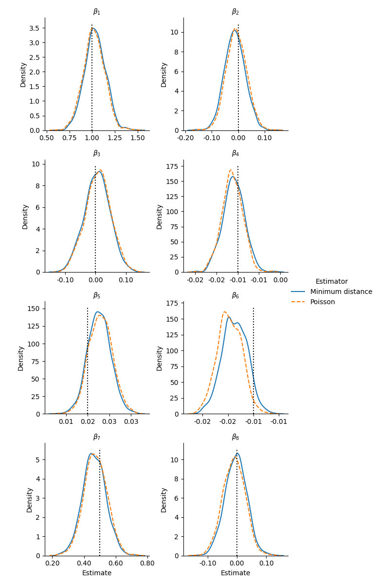
Figure 1: Estimating the Choo and Siow Model

4.2 Semilinear Nested Logit

For both men and women, we defined three nests that consist of $\{0\}$, $\{1,\ldots,10\}$, and $\{11,\ldots,20\}$. We take the true nest parameters to be all equal to $0.5$ (that is, $\rho_{n}^{x}=\delta_{n^{\prime}}^{y}=0.5$ for all $n,n^{\prime}:x\in n$ and $y\in n^{\prime}$).

To generate samples from the nested logit model, we proceed as with the logit model. The only difference is that setting up the system to be solved for equilibrium requires a bit more work. We describe our IPFP algorithm in Appendix A.

The minimum distance estimator converges fast on all samples. However, we found that a sample size of 10,000 households was much too small to get reliable estimates of the parameters. Figure 2 gives the distribution of the estimates of the four nest parameters (first two rows) and the eight coefficients of the bases for larger sample sizes: respectively $N=100,000$ and $N=1,000,000$. There is a clear downwards bias on the nest parameters $\rho$ and $\delta$ when $N=100,000$, to the point that some estimates are negative. Some of the coefficients of the bases are also badly estimated. With $N=1,000,000$, the minimum distance estimator performs much better.

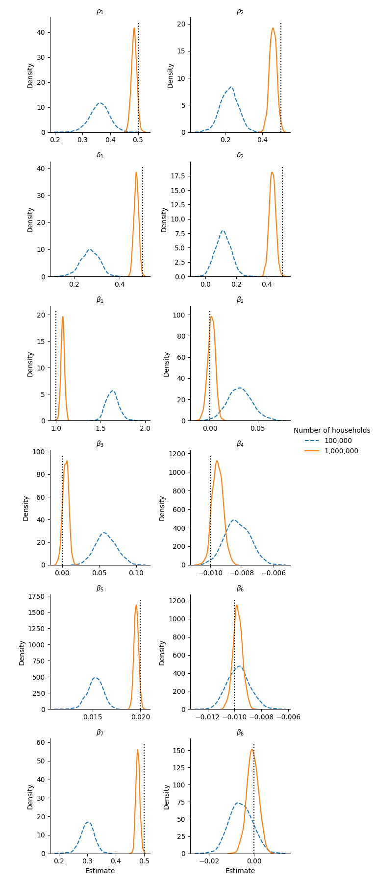
Figure 2: Estimating the Nested Logit Model

Concluding remarks

Each of the two methods we presented here has its pros and cons.

The minimum-distance estimator applies to all separable models; it is most convenient in semilinear models. To achieve maximum efficiency, and to test the specification, one needs to evaluate the second derivatives of the entropy with respect to the matching patterns. This may be difficult. In addition, the data often contains zero cells—some $\hat{\mu}_{xy}$ may be zero. Then the corresponding equation in (2.1) is only an inequality and it must be dropped from the system of estimating equations. An alternative is to add a small positive number $\delta$ to each $\hat{\mu}_{xy}$, to increase the margins $\hat{n}_{x}$ and $\hat{m}_{y}$ accordingly, and to estimate on this adjusted data.

The Poisson regression estimator only applies to semilinear [5] (choo-siow:06) models. It is appealing in its simplicity of use, as one can rely on standard statistical packages. It is also more robust to zero cells: nothing in Section 3 relied on taking derivatives with respect to $\bm{\mu}$ at the observed matching patterns.

Our simulations suggest that it takes large sample sizes to get reliable estimates of distributional parameters (our $\bm{\alpha}$). In labor markets or in marriage markets, large samples are readily available. When they are not (as with matching between firms), it may be better to stick to the [5] (choo-siow:06) specification. Fortunately, the simulations reported in [3] (cns:19) are encouraging as to its robustness.

Appendix A IPFP for the Nested Logit

Let us consider a nested logit model in which the nests do not depend on the type ($\mathcal{N}_{x}\equiv\mathcal{N}$ and $\mathcal{N}^{\prime}_{y}\equiv\mathcal{N}^{\prime}$) and their parameters $\bm{\rho}$ and $\bm{\delta}$ only depend on the nest: $\rho^{x}_{n}\equiv\rho_{n}$ and $\delta^{y}_{n^{\prime}}\equiv\delta_{n^{\prime}}$. Equation (2.2.2) can be rewritten as follows, for $y\in n$ and $x\in n^{\prime}$:

$$\mu_{xy}^{\rho_{n}+\delta_{n^{\prime}}}=\exp(\Phi_{xy})\mu_{x0}\mu_{0y}\mu_{xn}^{\rho_{n}-1}\mu_{n^{\prime}y}^{\delta_{n^{\prime}}-1}.$$ (A.1)

Since $\mu_{xn}=\sum_{y\in n}\mu_{xy}$, we get

$$\mu_{xn}=\mu_{x0}^{1/(\rho_{n}+\delta_{n^{\prime}})}\mu_{xn}^{(\rho_{n}-1)/(\rho_{n}+\delta_{n^{\prime}})}\sum_{y\in n}\exp\left(\Phi_{xy}/(\rho_{n}+\delta_{n^{\prime}})\right)\mu_{0y}^{1/(\rho_{n}+\delta_{n^{\prime}})}\mu_{n^{\prime}y}^{(\delta_{n^{\prime}}-1)/(\rho_{n}+\delta_{n^{\prime}})},$$

and, denoting $K_{xy}=\exp\left(\Phi_{xy}/(\rho_{n}+\delta_{n^{\prime}})\right)$:

$$\mu_{xn}^{(\delta_{n^{\prime}}+1)/(\rho_{n}+\delta_{n^{\prime}})}=\mu_{x0}^{1/(\rho_{n}+\delta_{n^{\prime}})}\sum_{y\in n}K_{xy}\mu_{0y}^{1/(\rho_{n}+\delta_{n^{\prime}})}\mu_{n^{\prime}y}^{(\delta_{n^{\prime}}-1)/(\rho_{n}+\delta_{n^{\prime}})}.$$ (A.2)

Substituting in the adding up constraint $\mu_{x0}+\sum_{y=1}^{Y}\mu_{xy}=n_{x}$ gives

$$n_{x} =\mu_{x0}+\sum_{n\in\mathcal{N}}\mu_{xn}$$

$$=\mu_{x0}+\sum_{n\in\mathcal{N}}\mu_{x0}^{1/(\delta_{n^{\prime}}+1)}\left(\sum_{y\in n}K_{xy}\mu_{0y}^{1/(\rho_{n}+\delta_{n^{\prime}})}\mu_{n^{\prime}y}^{(\delta_{n^{\prime}}-1)/(\rho_{n}+\delta_{n^{\prime}})}\right)^{(\rho_{n}+\delta_{n^{\prime}})/(\delta_{n^{\prime}}+1)}.$$ (A.3)

For given values of $(\mu_{0y},\mu_{n^{\prime}y})$ for all $y$, (A) defines $\mu_{x0}$ uniquely . Once $\mu_{x0}$ is known, we can plug it in (A.2) to obtain the values of $\mu_{xn}$ for all $n$. We do this for all values of $x$.

Then we can apply similar equations to the $y$ side:

$$\mu_{n^{\prime}y}^{(\rho_{n}+1)/(\rho_{n}+\delta_{n^{\prime}})} =\mu_{0y}^{1/(\rho_{n}+\delta_{n^{\prime}})}\sum_{x\in n^{\prime}}K_{xy}\mu_{x0}^{1/(\rho_{n}+\delta_{n^{\prime}})}\mu_{xn}^{(\rho_{n}-1)/(\rho_{n}+\delta_{n^{\prime}})}$$

$$m_{y} =\mu_{0y}+\sum_{n^{\prime}\in\mathcal{N}^{\prime}}\mu_{0y}^{1/(\rho_{n}+1)}\left(\sum_{x\in n^{\prime}}K_{xy}\mu_{x0}^{1/(\rho_{n}+\delta_{n^{\prime}})}\mu_{xn}^{(\rho_{n}-1)/(\rho_{n}+\delta_{n^{\prime}})}\right)^{(\rho_{n}+\delta_{n^{\prime}})/(\rho_{n}+1)}$$

to solve for $\mu_{0y}$ and $\mu_{n^{\prime}y}$ given the values of $(\mu_{x0},\mu_{xn})$ for all $x$. We iterate until convergence and we use (A.1) to compute the matching patterns $\mu_{xy}$.

Appendix B Proofs

B.1 Proof of theorem 1

Recall that

$$N=\sum_{x,y}\mu_{xy}^{\bm{\beta}}+\sum_{x}\mu_{x0}^{\bm{\beta}}+\sum_{y}\mu_{0y}^{\bm{\beta}}$$

is the total mass of households in the sample. For the [5] (choo-siow:06) specification we have at the stable matching $(\bm{\mu},\bm{u},\bm{v})$ for a joint surplus $\bm{\Phi}^{\bm{\beta}}$:

$$\mu_{x0} =\hat{n}_{x}\exp(-u_{x})$$

$$\mu_{0y} =\hat{m}_{y}\exp(-v_{y})$$ (B.1)

$$\mu_{xy} =\sqrt{\hat{n}_{x}\hat{m}_{y}}\exp((\Phi_{xy}-u_{x}-v_{y})/2).$$

Consider the maximization of the following expression:

$$\sum_{x,y}\hat{\mu}_{xy}\bm{\phi}_{xy}\bm{\beta}-2\sum_{x,y}\sqrt{\hat{n}_{x}\hat{m}_{y}}\exp((\bm{\phi}_{x}\bm{\beta}-u_{x}-v_{y})/2)$$

$$\ -\sum_{x}\hat{n}_{x}\exp(-u_{x})-\sum_{y}\hat{m}_{y}\exp(-v_{y})-\sum_{x}\hat{n}_{x}u_{x}-\sum_{y}\hat{m}_{y}v_{y}$$

over $\bm{u}$, $\bm{v}$, and $\bm{\beta}$. We see that the first order conditions yield that $\bm{\mu}$ defined in B.1 satisfies the margin equations

$$\sum_{y}\mu_{xy}+\mu_{x0}=n_{x}$$ (B.2)

$$\sum_{x}\mu_{xy}+\mu_{0y}=m_{y}$$ (B.3)

for the first order conditions with respect to $u_{x}$ and $v_{y}$, and

$$\sum_{xy}\mu_{xy}\phi_{xy}^{k}=\sum_{xy}\hat{\mu}_{xy}\phi_{xy}^{k}$$

for the first order conditions with respect to $\beta_{k}$.

Now remember that the log-likelihood function of a Poisson count model with parameter $\exp(\bm{Z}_{a}^{\top}\bm{\gamma})$ is

$$l\left(\bm{\hat{\mu}},\bm{\gamma};\bm{w}\right)=\sum_{a\in\mathcal{A}}w_{a}\left(\hat{\mu}_{a}\bm{Z}^{\top}_{a}\bm{\gamma}-\exp\left(\bm{Z}^{t}op_{a}\bm{\gamma}\right)-\log(\hat{\mu}_{a}!)\right).$$ (B.4)

if the observations $(\hat{N}_{a},\bm{Z}_{a})_{a\in\mathcal{A}}$ are weighted by a vector $\bm{w}$. Define $\bm{\gamma}=(\bm{\beta}^{\top},\bm{a}^{\top},\bm{b}^{\top})$ with

$$\bm{a}=\bm{u}-\log\bm{\hat{n}},\;\;\bm{b}=\bm{v}-\log\bm{\hat{m}}.$$

Then with $\bm{Z}$ and $\bm{w}$ defined in Theorem (1), we have

$$\left(\bm{Z}\bm{\gamma}\right)_{xy} =(\bm{\phi}_{xy}\bm{\beta}-u_{x}+\log\hat{n}_{x}-v_{y}+\log\hat{m}_{y})/2$$

$$\left(\bm{Z}\bm{\gamma}\right)_{x} =-u_{x}+\log\hat{n}_{x}$$

$$\left(\bm{Z}\bm{\gamma}\right)_{y} =-v_{y}+\log\hat{m}_{y};$$

and up to constant terms, $l$ and $L$ are identical.

B.2 Proof of theorem 2

The variance-covariance matrix of $\hat{\bm{\gamma}}$ follows directly from the fact that it maximizes (B.4), and hence is an M-estimator, see chapter 5 of [8] (vaart:1998). The maximization of (B.4) gives first-order conditions

$$\sum_{a\in\mathcal{A}}w_{a}\exp(\bm{Z}_{a}\hat{\bm{\gamma}})\bm{Z}_{a}=\sum_{a\in\mathcal{A}}w_{a}\hat{\mu}_{a}\bm{Z}_{a},$$

so that, applying the delta method, we get at first order

$$\left(\sum_{a\in\mathcal{A}}w_{a}\exp(\bm{Z}_{a}\hat{\bm{\gamma}})\bm{Z}_{a}^{\top}\bm{Z}_{a}\right)(\hat{\bm{\gamma}}-\bm{\gamma})=\sum_{a\in\mathcal{A}}w_{a}\bm{Z}_{a}(\hat{\mu}_{a}-\mu_{a}).$$

so we obtain a consistent estimator of the variance of $\bm{\hat{\gamma}}$ as

$$\hat{V}\hat{\bm{\gamma}}=\bm{\hat{A}}^{-1}\;\hat{\bm{B}}\;\bm{\hat{A}}^{-1}$$

where

$$\bm{\hat{A}}=\sum_{a\in\mathcal{A}}w_{a}\exp(\bm{Z}_{a}\hat{\bm{\gamma}})\bm{Z}_{a}^{\top}\bm{Z}_{a}$$

and

$$\bm{\hat{B}}=\sum_{a,a^{\prime}\in\mathcal{A}}w_{a}w_{a^{\prime}}\mbox{cov}(\hat{\mu}_{a},\hat{\mu}_{a^{\prime}})\bm{Z}^{\top}_{a}\bm{Z}_{a^{\prime}}.$$

References

• [1] S. Berry, J. Levinsohn and A. Pakes “Automobile Prices in Market Equilibrium” In Econometrica 63, 1995, pp. 841–890
• [2] S. Berry and A. Pakes “The Pure Characteristics Demand Model” In International Economic Review 48, 2007, pp. 1193–1225
• [3] P.-A. Chiappori, D.. Nguyen and B. Salanié “Matching with Random Components: Simulations” Columbia University mimeo, 2019
• [4] P.-A. Chiappori, B. Salanié and Y. Weiss “Partner Choice, Investment in Children, and the Marital College Premium” In American Economic Review 107, 2017, pp. 2109–67
• [5] E. Choo and A. Siow “Who Marries Whom and Why” In Journal of Political Economy 114, 2006, pp. 175–201
• [6] A. Galichon and B. Salanié “Cupid’s Invisible Hand: Social Surplus and Identification in Matching Models” forthcoming In Review of Economic Studies, 2022
• [7] J… Santos Silva and Silvana Tenreyro “The Log of Gravity” In Review of Economics and Statistics 88, 2006, pp. 641–658
• [8] A. Vaart “Asymptotic Statistics” Cambridge University Press, 1998